Random graphs from random matrices

Abstract.

In the paper [GPCI15], the authors introduced the order complex corresponding to a symmetric matrix. In this note, we use it to define a class of models of random graphs, and show some surprising experimental results, showing sharp phase transitions.

1. Introduction

In the paper [GPCI15] the authors introduce the ”order complex” associated to a (symmetric) matrix. Briefly, we view the symmetric $n\times n$ matrix $M$ (with its diagonal set to zero) as the adjacency matrix of the complete graph $K_{n},$ and now we produce an increasing family of graphs, starting with the completely disconnected graph on $n$ vertices, and then adding edges in order of increasing size of the corresponding entry of the matrix $M,$ until $p*n(n-1)/2$ edges have been added (in other words, the edge density in the graph is $p$). It is now natural to look at different models of random matrices, use them to generate random graphs, and see what the properties of the random graphs are.

Example 1.1.

Suppose $M$ is drawn from the ensemble of symmetric matrices with i.i.d Gaussian entries (note: for this model it is irrelevant what the mean of the Gaussian is). Then the random graphs are nothing but the much studied Erdös-Rényi random graphs.

Example 1.2.

In the upcoming paper [CR19] we generate a random vector $v$ and look at the rank one matrix $M(v)=v^{t}v$ - in the case where the entries of $v$ are iid $\mathcal{N}(0,1),$ this is a Wishart ensemble. However, if we pick the entries of $v$ to be uniform in $[0,1],$ we get a model with other properties .

Example 1.3.

This is, in a way, the motivating example: consider a point cloud approximating some shape in $\mathbb{R}^{n}$ (usually for $n=2,3$), and let $M$ be the distance matrix of this cloud (that is, the $M_{ij}$ equals the distance between the $i$th and the $j$th points in the cloud.

In this paper we look at the Laplacian eigenvalues of the graphs we construct. There are (at least) two ways to define the Laplacian matrix of a graph. The first, and simplest is

$$L=D-A,$$

where $D$ is the diagonal matrix of degrees of vertices and $A$ is the adjacency matrix of the graph $G.$ The second is the normalized symmetric Laplacian (see [CG97]):

$$\mathcal{L}=D^{-\frac{1}{2}}LD^{-\frac{1}{2}},$$

with $L$ as above.

It turns out that the normalized Laplacian is much better behaved. Note that the normalized Laplacian spectrum is contained between $0$ and $2,$ and the mean is at $1,$ since the trace of $\mathcal{L}$ is always equal to $n.$

2. Spectral Gap

2.1. Erdös-Rényi model

.

(a) Raw spectral gap

(b) Normalized spectral gaps.

Figure 1. ER Model

We see that the “raw” spectral gap - Figure 1(a) increases linearly from $0$ to the value of the complete graph ($K_{2}000$ in this case), while the normalized gap - Figure 1(b) - is asymptotic to $1.$ The latter case has been studied - $\lambda_{2}\asymp C1-Cn^{-\frac{1}{2}},$ see [HKP19], but the former seems to be a new observation.

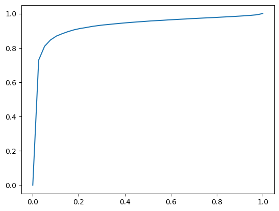
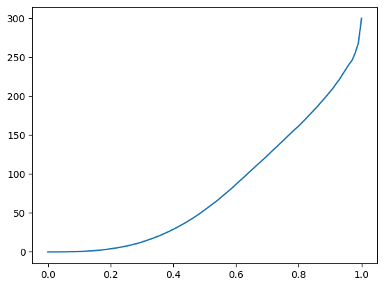
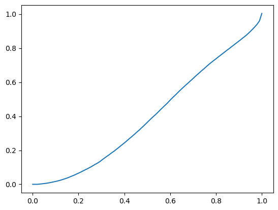
2.2. Positive rank one model

(a) Raw spectral gap

(b) Normalized spectral gap

Figure 2. positive rank 1

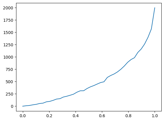
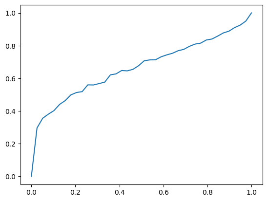
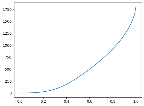
We notice that the raw spectral gap - Figure 2(a)- seems to increase like $\sqrt{p},$ while the normalized gap - Figure 2(b) - is increasing linearly to $1.$ To confirm the first observation, let us plot the square root of the gap:

Figure 3. Square root of raw spectral gap for positive rank 1 model

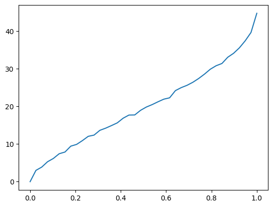
Note that Figure 3 is consistent with quadratic growth of the spectral gap. It is also interesting that the two ends (near the completely disconnected and complete graphs) seem symmetric.

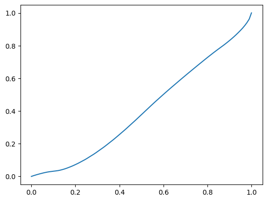
2.3. Rank 1 Wishart model

(a) Raw spectral gap

(b) Normalized spectral gaps

Figure 4. Wishart rank 1

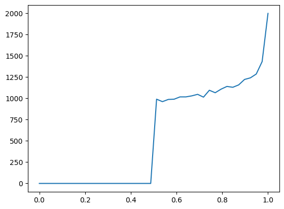
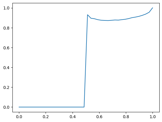
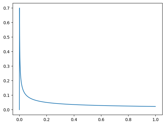
The evolution of the spectral gap (see Figure 4) looks starkly different in the Wishart model. Part of the explanation is that (as noted in [CR19]), the graph stays bipartite for low density, until at (roughly) density $p=\frac{1}{2}$ it becomes complete bipartite (recall that the Laplace eigenvalues of $K_{m,n}$ are $m+n,n,m,0,$ with multiplicities $1,m-1,n-1,1.$ However, this explains only some of the features of the evolution (in particular, the sharp phase transition just before the graph becomes complete bipartite and the non-monotonicity of the function).

2.4. Point clouds

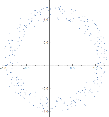
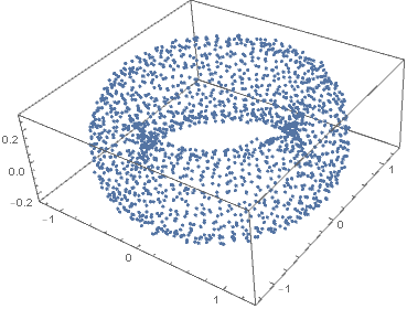
We now look at the ”motivating examples” - point clouds in low-dimensional spaces. The point clouds we look at are the noisy circle and the noisy torus, both found in the Eirene ([HG16]) distribution - see Figures 5(a) and 5(b).

(a) Noisy circle

(b) Noisy torus.

We convert these point clouds into distance matrices, and see the following spectral behavior:

(a) Raw spectral gap

(b) Normalized spectral gap

Figure 6. Noisy circle spectral curves

(a) Raw spectral gap

(b) Normalized spectral gap

Figure 7. Noisy torus spectral curves

It is quite obvious to the naked eye that the spectral gap curves in Figures 6 and 7 are very similar to those in the positive rank one case (Figure 2

3. Spectral densities

3.1. Erdös-Rényi

The spectral density of the Erdös-Rényi random graph has been extensively studied (see, for example [EKY⁺13]) - the ”raw” spectrum seems to have been more extensively studied, and found to satisfy the semicircle law (as the reader might be convinced by looking at the figures 8 and 9).

(a) Raw spectral density

(b) Normalized spectral density

Figure 8. Spectral density at $p=0.05$

(a) Raw spectral density

(b) Normalized spectral density

Figure 9. Spectral density at $p=0.2$

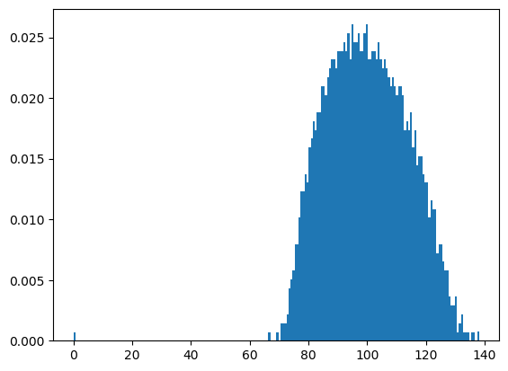
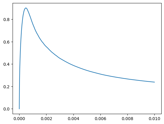
We see that the shapes (whatever that means) of the curves stabilize fairly quickly, and only the width is shrinking with increasing $p.$ it is thus natural to look at the width as a function of $p.$ Instead of the width (which is a little hard to define, we just look at the standard deviation of the empirical distribution of eigenvalues. Let us do it for the normalized spectrum:

(a) Entire graph

(b) Zoom around maximum

Figure 10. Standard deviation of spectral density

We see in Figure 10 that the standard deviation rises sharply until $p=1/n,$ and then declines.

3.2. Positive rank 1

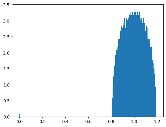
First let us look at the spectral distribution:

(a) Raw spectral distribution,

(b) Normalized spectral distribution

Figure 11. Positive rank 1 model , $p=0.05$

(a) Raw spectral distribution,

(b) Normalized spectral distribution

Figure 12. Positive rank 1 model , $p=0.2$

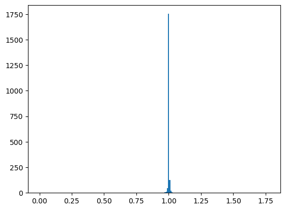
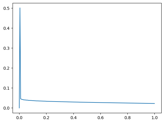
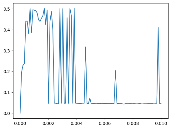
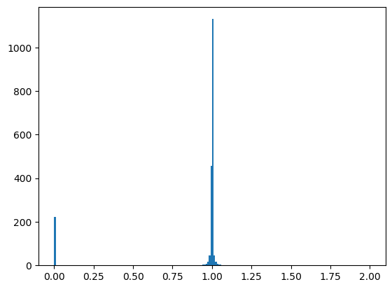
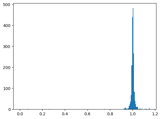
The raw distribution is interesting (there is a large spike at $n$), but what is more interesting is that the normalized Laplacian has extreme concentration of eigenvalues at $1,$ completely unlike the Erdös-Rényi model. The standard deviation of the spectral distribution is (not surprisingly) much smaller, and it is also much less regular, the peak is also achieved for a far larger $p.$

(a) Entire graph

(b) Zoom around maximum

Figure 13. Standard deviation of spectral density for positive rank 1 model

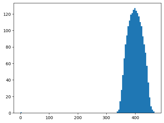
3.3. Wishart rank 1

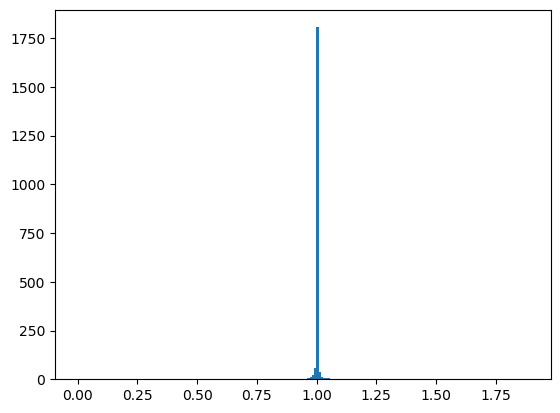
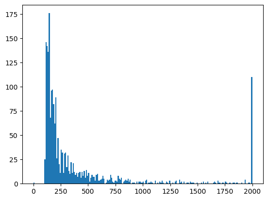
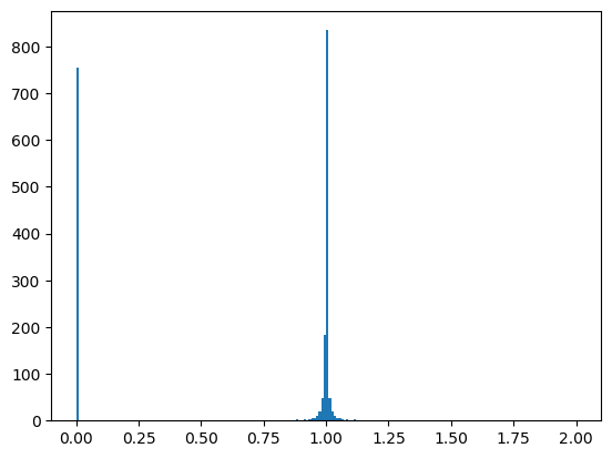
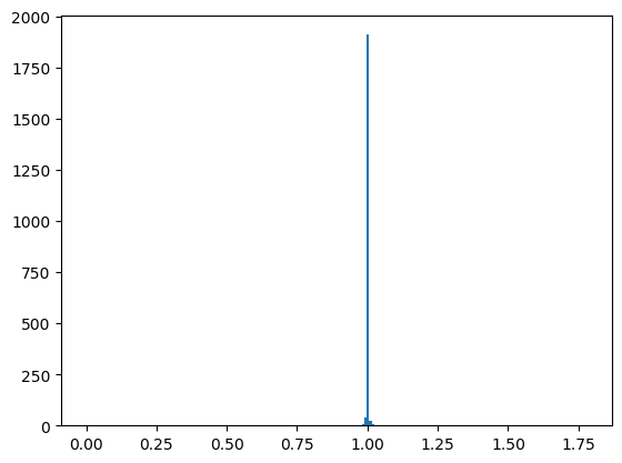
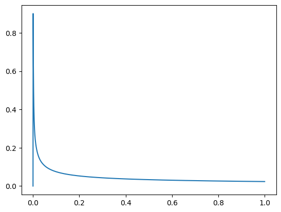
The Wishart rank one graphs show essentially the same behavior as the positive rank one case, with a very tight concentration around $1,$ and rapid decay, but also a massive concentration at $0$ (indicating many connected components) for $p<0.5$ See Figure 14.

(a) $p=0.05$

(b) $p=0.2$

(c) $p=0.6$

Figure 14. Spectral density of Wishart rank 1 model

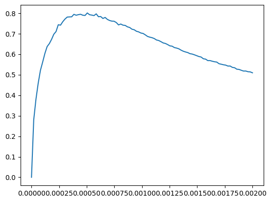
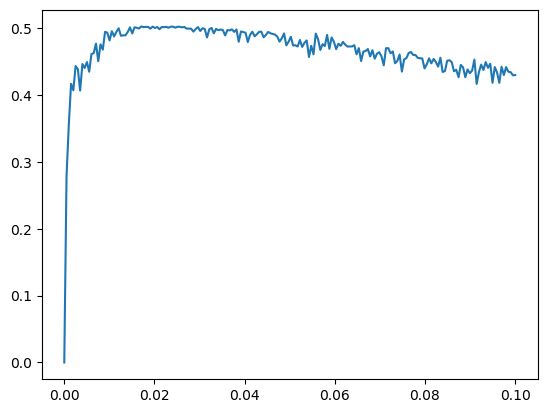
The standard deviation is quite different from the positive case - see Figure 15 - showing the usual phase transition at $p=0.5$

(a) Entire graph

(b) Zoom around maximum

Figure 15. Standard deviation of spectral density for Wishart rank 1 model

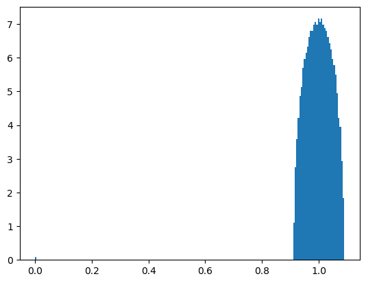
3.4. Point Clouds

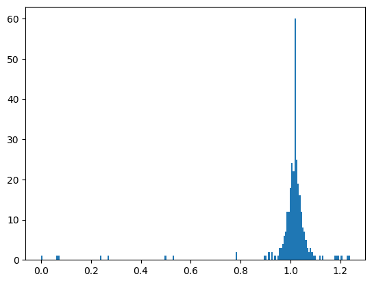
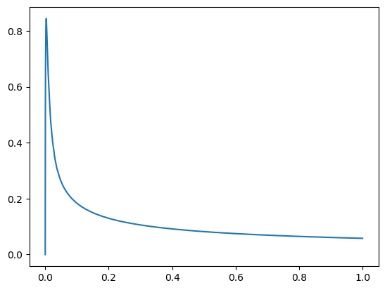
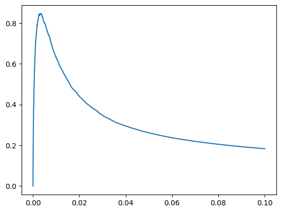
Here we look at the spectral distribution of the point clouds (noisy circle and noisy torus). It is evident that these are very close to the positive rank one matrices - the reader can judge for his or her own self. The bulk density at $p=0.2$ is in Figure 16

(a) Noisy circle

(b) noisy torus

Figure 16. Spectral density at $p=0.2$l

The evolution of standard deviation for the circle is given in Figure 17, for the torus in Figure 18.

(a) Entire graph

(b) Zoom around maximum

Figure 17. Standard deviation of spectral density for noisy circle

(a) Entire graph

(b) Zoom around maximum

Figure 18. Standard deviation of spectral density for noisy torus

References

- [CG97] Fan RK Chung and Fan Chung Graham. Spectral graph theory. Number 92. American Mathematical Soc., 1997.
- [CR19] Carina Curto and Igor Rivin. Rank one complexes - exactly solved models in topological data analysis. 2019. In preparation.
- [EKY+13] László Erdős, Antti Knowles, Horng-Tzer Yau, Jun Yin, et al. Spectral statistics of erdős–rényi graphs i: local semicircle law. The Annals of Probability, 41(3B):2279–2375, 2013.
- [GPCI15] Chad Giusti, Eva Pastalkova, Carina Curto, and Vladimir Itskov. Clique topology reveals intrinsic geometric structure in neural correlations. Proceedings of the National Academy of Sciences, 112(44):13455–13460, 2015.
- [HG16] G. Henselman and R. Ghrist. Matroid Filtrations and Computational Persistent Homology. ArXiv e-prints, June 2016.
- [HKP19] Christopher Hoffman, Matthew Kahle, and Elliot Paquette. Spectral Gaps of Random Graphs and Applications. International Mathematics Research Notices, 05 2019.