Warm Start of Mixed-Integer Programs
for Model Predictive Control of Hybrid Systems

Abstract

In hybrid Model Predictive Control (MPC), a Mixed-Integer Quadratic Program (MIQP) is solved at each sampling time to compute the optimal control action. Although these optimizations are generally very demanding, in MPC we expect consecutive problem instances to be nearly identical. This paper addresses the question of how computations performed at one time step can be reused to accelerate (warm start) the solution of subsequent MIQPs.

Reoptimization is not a rare practice in integer programming: for small variations of certain problem data, the branch-and-bound algorithm allows an efficient reuse of its search tree and the dual bounds of its leaf nodes. In this paper we extend these ideas to the receding-horizon settings of MPC. The warm-start algorithm we propose copes naturally with arbitrary model errors, has a negligible computational cost, and frequently enables an a-priori pruning of most of the search space. Theoretical considerations and experimental evidence show that the proposed method tends to reduce the combinatorial complexity of the hybrid MPC problem to that of a one-step look-ahead optimization, greatly easing the online computation burden.

I Introduction

Model Predictive Control (MPC) is a numerical technique that enables the design of optimal feedback controllers for a wide variety of dynamical systems [1, 2]. The main idea behind it is straightforward: if we are able to solve trajectory optimization problems quickly enough, we can replan the future motion of the system at each sampling time and achieve a reactive behavior. While for smooth dynamics the online computations of MPC are generally limited to a simple convex program (even in the nonlinear case [3]), the discrete behavior of hybrid systems is most naturally modeled with integer variables, requiring the real-time solution of mixed-integer programs. This can be prohibitive even for systems with “slow dynamics” and of “moderate size.”

The focus of this paper is hybrid linear systems, i.e., systems whose nonlinearity is exclusively due to discrete logics. For these, in the common case of a quadratic cost, the MPC problem falls in the class of Mixed-Integer Quadratic Programs (MIQPs). MIQPs are NP-hard problems and, as such, no polynomial-time algorithm is known for their solution. The most robust and effective strategy for tackling this class of optimizations is Branch and Bound (B&B) [4, 5]. Despite its worst-case performance, this algorithm is very appealing: for a feasible optimization, B&B converges to a global optimum; otherwise, it provides a certificate of infeasibility.

B&B solves an MIQP by constructing a search tree, where at each node a Quadratic Program (QP) is solved to bound the objective function over a subset of the search space. As an order of magnitude, for large-scale control problems, B&B can easily require millions of QPs to converge [6]. It is therefore natural to ask whether at the end of the time step all the information contained in the tree is necessarily lost, or it can be reused to warm start the solution of the next MIQP. This seems plausible considering that two consecutive optimizations overlap for most of the time horizon, and differ only for a one-step shift of the time window. This idea has been extremely successful in linear MPC (see, e.g., [7, 8, 9, 10, 11]), but its application in the hybrid case raises many difficulties and has been obstructed by the complexity of B&B algorithms.

I-A Related Works

Given the difficulty of solving MIQPs online, techniques to compute offline the optimal control as a function of the system state have been intensively developed [12, 13, 14], and also extended beyond hybrid linear systems [15, 16]. However, the application of these explicit methods is typically limited to low-dimensional systems, with very few discrete variables. Approximate explicit solutions to the hybrid MPC problem have been proposed in [17, 18, 19]. These extend the scope of exact approaches, but still require a substantial amount of offline computations, which might not be feasible in many applications. In fact, certain problem data might be known only at run time, excluding the possibility of solving the MPC problem offline.

Noticing that the hardness of these problems lies in the identification of the optimal integer assignment, one can devise a split of the problem into two: a cheap algorithm to generate a good guess for the integers, followed by a rounding step [20, 21, 22, 23]. This is a popular approach for hybrid nonlinear systems, and warm starting is having a crucial role in its advancement [24]. However, it is not particularly convenient in our context, since the rounding step above typically suffers from the same combinatorics as our original MIQP.

Even though heuristic [25] and local [26] methods have recently been proved to be very effective, B&B is still the most reliable algorithm for solving hybrid MPC problems online [27, Section 17.4]. Many enhancements of B&B tailored to MPC have been proposed, and attention has been mainly focused on accelerating the solution of the quadratic subproblems. To this end, various algorithms have been considered: dual active set [28], dual gradient projection [29, 30], interior point [23], partially-nonnegative least squares [31, 32], and alternating-direction method of multipliers [33]. Search heuristics that leverage the problem temporal structure have also been proposed [34, 23].

Most of the B&B schemes mentioned above make full use of warm start within a single B&B solve, using the parent solution as a starting point for the child subproblems. However, the issue of reusing computations across time steps has only been discussed in [32]. There, a guess of the optimal integer assignment (obtained by shifting the previous solution) is prioritized within the construction of the new tree. A similar approach has recently been proposed in [35], where the whole path from the B&B root to the optimal leaf is propagated in time. Even if these techniques can lead to considerable savings, limiting the data propagated across time steps to a guess of the optimal solution is generally very restrictive. In fact, in practice, we often expect disturbances to make these guesses inaccurate. More importantly, even in the ideal case in which the integer warm start is actually optimal, these methods still build a B&B tree almost from scratch, requiring the solution of many subproblems. Note that, for an MIQP, proving optimality of a candidate solution is in principle as hard as solving the original optimization [36].

The problem of warm starting (or reoptimizing) a Mixed-Integer Linear Program (MILP) is not new to the operations research community [37]. For a sequence of MILPs with common constraint matrix, the general approach is to start each B&B search from the final frontier (B&B leaves) of the previous solver run [38, 39]. Moreover, in case of changes in the constraint right-hand side only, the dual bases of the previous frontier can be used to bound the optimal values of the new leaves [40]. This is a much more comprehensive reuse of computations than what is currently done in MPC. First, not only the optimal solution, but the whole B&B tree is propagated between subsequent problems. This is very important, since, before convergence, the B&B algorithm might also need to thoroughly explore regions of the search space that are far away from the optimum. Second, by propagating dual bounds between consecutive MILPs, these approaches are capable of pruning large branches of the tree without solving any subproblems.

The latter ideas do not transfer smoothly to MPC. In the general case of a time-varying system, consecutive MPC problems do not share the same constraint matrix, and the techniques mentioned above do not apply. In the time-invariant case, on the other hand, we could interpret a sequence of MPC problems as MIQPs with variable constraint right-hand side, as done in explicit MPC [41, 13]. However, proceeding as in [40], B&B solutions would be reused without being shifted in time, completely ignoring the receding-horizon structure of the problem at hand.

I-B Contribution

We present a novel warm-start procedure for hybrid MPC, which bridges the gap with state-of-the-art reoptimization techniques from operations research. First, we show how an initial search frontier for the hybrid MPC problem can be obtained by shifting in time part of the final frontier of the previous B&B tree. Then, duality is used to derive tight bounds on the cost of the new subproblems. Starting from this refined partition of the search space, B&B generally requires only a few subproblems to find the optimum. Then, the implied dual bounds readily prune most of the search space, accelerating convergence without sacrificing global optimality. Neither the shift of the B&B frontier, nor the synthesis of the bounds, causes any significant time overhead in the MIQP solves.

The proposed method copes naturally with model errors and disturbances of any magnitude. Remarkably, as the time horizon grows, and the MPC policy becomes stationary, our approach reduces the hybrid MPC combinatorics to that of a one-step look-ahead problem. In this asymptotic case, previous computations are fully reused and only the variables of the final time step have to be reoptimized.

We evaluate the performance of our algorithm with a thorough statistical analysis. In the vast majority of the cases, it leads to a drastic reduction of computation times and, even in the worst case, it still performs better than the customary approach of solving each MIQP from scratch.

I-C Article Organization

We structured this paper trying to maximize readability. We start in Section II presenting a minimal formulation of the MPC problem, which contains only the components necessary to the development of the warm-start algorithm. Section III reviews the B&B algorithm, emphasizing the advantages of dual methods in the solution of the subproblems. In the same section, we identify the three main ingredients that compose a warm start for an MIQP. Sections IV, V, and VI are devoted to showing how each of these ingredients can be efficiently computed for the minimal MPC problem at hand. Section VII presents an asymptotic analysis of the algorithm as the MPC time horizon tends to infinity. In Section VIII we generalize the problem formulation from Section II, and we extend the results to these more general settings. A statistical study of the algorithm performance is reported in Section IX. Section X is dedicated to conclusions. In Appendix A several extensions of the proposed warm-start method are discussed, whereas Appendices B and C contain mathematical derivations.

I-D Notation

We denote the set of real numbers as $\mathbb{R}$ and, e.g., nonnegative reals as $\mathbb{R}_{\geq 0}$. The same notation is used for integers $\mathbb{Z}$, and we let $\mathbb{N}:=\mathbb{Z}_{\geq 0}$. The Euclidean length of a vector $x\in\mathbb{R}^{n}$ is $|x|$. We use the same symbol for the cardinality $|\mathcal{S}|$ of a set $\mathcal{S}$. For two vectors $x\in\mathbb{R}^{n}$ and $y\in\mathbb{R}^{m}$, $(x,y)\in\mathbb{R}^{n+m}$ represents their concatenation. For a matrix $A\in\mathbb{R}^{n\times m}$, we let $A^{\prime}$ be its transpose, $A^{+}$ its pseudoinverse, $\|A\|$ its maximum singular value, and $\ker(A)$ its nullspace. All physical units may be assumed to be expressed in the MKS system.

II Hybrid Model Predictive Control

Many equivalent descriptions of hybrid linear systems can be found in the literature [42], in this paper we employ the popular framework of Mixed Logical Dynamical (MLD) systems [2]. This description naturally lends itself to mixed-integer optimization, and it is the intermediate representation in which hybrid systems are more commonly cast for numerical optimal control [27, Section 17.4]. In this section, we introduce MLD systems (Section II-A) and we formulate the associated MPC problem (Section II-B).

II-A Mixed Logical Dynamical Systems

We compactly represent an MLD system as

$$x_{\tau+1}=Ax_{\tau}+Bu_{\tau}+e_{\tau},\quad(x_{\tau},u_{\tau})\in\mathcal{D},$$ (1)

where $x_{\tau}\in\mathbb{R}^{n_{x}}$ denotes the system state at discrete time $\tau\in\mathbb{N}$, $u_{\tau}\in\mathbb{R}^{n_{u}}\times\{0,1\}^{m_{u}}$ collects continuous and binary inputs, $e_{\tau}\in\mathbb{R}^{n_{x}}$ represents the model error, and the domain $\mathcal{D}:=\{(x,u)\mid Fx+Gu\leq h\}$ is a polyhedral subset of $\mathbb{R}^{n_{x}+n_{u}+m_{u}}$ which contains the origin. We denote by $v_{\tau}\in\{0,1\}^{m_{u}}$ the binary entries in the input vector, and we let $V$ be the selection matrix such that $v_{\tau}=Vu_{\tau}$.

Even if the MLD model (1) is more compact than the usual description employed in the MPC literature, it can be used without loss of generality:

• Often a distinction between independent and dependent (auxiliary) input variables $u_{\tau}$ is made [2]. For a well-posed MLD system, the second are assumed to be uniquely determined by the first and the state $x_{\tau}$ through the constraint set $\mathcal{D}$. However, the role of these variables is identical from the optimization viewpoint, so we do not distinguish between them here.

• Affine MLD dynamics as in [27, Section 16.5] can be made linear through a shift of the system coordinates around an equilibrium point $(\hat{x},\hat{u})$, provided that binary inputs are defined so that $V\hat{u}=0$.

• Binary states can be handled introducing auxiliary inputs. Let $A_{i}$ and $B_{i}$ be the $i$th rows of $A$ and $B$, respectively, and let $u_{\tau,j}\in\{0,1\}$ be the $j$th input. Enforcing $A_{i}x_{\tau}+B_{i}u_{\tau}=u_{\tau,j}$ through the constraint set $\mathcal{D}$, we obtain $x_{\tau+1,i}\in\{0,1\}$.

Handling binary states with auxiliary inputs simplifies the analysis but can be computationally inefficient: Appendix A-A shows how our warm-start algorithm can cope directly with binary states. Moreover, paying the price of a heavier notation, the proposed method also applies to time-varying MLD systems. This extension is presented in Appendix A-B.

II-B The Optimal Control Problem

We now describe the optimization problem beneath the hybrid MPC controller. To streamline the presentation, in the main body of this paper, we consider the simplified problem statement (2) given below. This formulation does not allow terminal penalties and constraints, which are fundamental tools to ensure the stability of the closed-loop system [1]. In Section VIII we extend our algorithm to incorporate these important MPC ingredients. Additionally, in this paper, we limit our attention to quadratic objective functions, even though the results we present can be easily adjusted in case of different convex costs (e.g., 1-norm or $\infty$-norm).

Under the assumption of a perfect model ($e_{\tau}=0$ for all $\tau$), an MPC controller regulates system (1) to the origin by solving an open-loop optimal control problem at each time step. Let $\tau$ be the time step at which the optimization problem is solved (the current time), and let $t\in\mathbb{N}$ denote the relative time within the MPC problem. Given the current state $x_{\tau}$, we formulate the MIQP

$$\min\ \sum_{t=0}^{T}|Qx_{t\mid\tau}|^{2}+\sum_{t=0}^{T-1}|Ru_{t\mid\tau}|^{2}$$ (2a)

$$\mathrm{s.t.}\ x_{0\mid\tau}=x_{\tau},$$ (2b)

$$x_{t+1\mid\tau}=Ax_{t\mid\tau}+Bu_{t\mid\tau}, t=0,\ldots,T-1,$$ (2c)

$$(x_{t\mid\tau},u_{t\mid\tau})\in\mathcal{D}, t=0,\ldots,T-1,$$ (2d)

$$Vu_{t\mid\tau}\in\{0,1\}^{m_{u}}, t=0,\ldots,T-1.$$ (2e)

Here the optimization variables are $\{u_{t\mid\tau}\}_{t=0}^{T-1}$ and $\{x_{t\mid\tau}\}_{t=0}^{T}$, and the time horizon $T$ is assumed to be fixed (the case with variable horizon is briefly discussed in Appendix A-C). We do not assume the objective (2a) to be strictly convex, i.e., the weight matrices $Q$ and $R$ are allowed to be rank deficient.

The outcome of (2) is an optimal (up to a tolerance $\varepsilon\in\mathbb{R}_{\geq 0}$) open-loop control sequence $\{u_{t\mid\tau}^{*}\}_{t=0}^{T-1}$, with the related state trajectory $\{x_{t\mid\tau}^{*}\}_{t=0}^{T}$. In MPC, only the first action $u_{\tau}:=u_{0\mid\tau}^{*}$ is applied to the system. Then, at time step $\tau+1$, the new current state $x_{\tau+1}$ is measured and problem (2) is solved in a receding-horizon fashion. Given the similarity of the problems we solve at time $\tau$ and $\tau+1$, it is natural to ask whether part of the computations performed at one time step can be exploited to speed up the solution of the consecutive problem. In the next section we introduce the notions necessary to formalize this question.

III Hybrid MPC via Branch-and-Bound

This section reviews the bases of B&B by considering its application to problem (2). In Section III-A, we describe the main steps of the algorithm. Placing a special emphasis on the input-output behavior of each iteration, we provide a simple formalization of the warm-start problem. In Section III-B, we discuss how Lagrangian duality can facilitate the solution of the B&B subproblems. For a more thorough description of B&B, we refer the reader to, e.g., [4, Section 9.2].

III-A The Branch-and-Bound Algorithm

Generally, B&B is presented as a tree search, where each node corresponds to a convex relaxation of the MIQP. Here we emphasize the set-cover interpretation of B&B, which enables a more fluent analysis of the warm-start problem. Similar presentations can also be found in [38, 39].

We denote problem (2) by $\mathbf{P}$ and its optimal value by $\theta\in\mathbb{R}_{\geq 0}\cup\{\infty\}$, where $\theta=\infty$ in case of an infeasible MIQP. In this section, for simplicity, we do not explicitly annotate the dependence of problem $\mathbf{P}$ on the time step $\tau$. The B&B search relies on the solution of convex relaxations (or subproblems) of $\mathbf{P}$, where the nonconvex constraints (2e) are replaced by the linear inequalities

$$\underaccent{\bar{}}{v}_{t\mid\tau}\leq v_{t\mid\tau}:=Vu_{t\mid\tau}\leq\bar{v}_{t\mid\tau},$$ (3)

for some $\underaccent{\bar{}}{v}_{t\mid\tau},\bar{v}_{t\mid\tau}\in\{0,1\}^{m_{u}}$ such that $\underaccent{\bar{}}{v}_{t\mid\tau}\leq\bar{v}_{t\mid\tau}$. A convex relaxation of $\mathbf{P}$ is hence a QP identified by the interval

$$\mathcal{V}:=[(\underaccent{\bar{}}{v}_{t\mid\tau})_{t=0}^{T-1},(\bar{v}_{t\mid\tau})_{t=0}^{T-1}]\subset\mathbb{R}^{Tm_{u}},$$ (4)

and we denote it by $\mathbf{P}(\mathcal{V})$. Similarly, $\theta(\mathcal{V})\in\mathbb{R}_{\geq 0}\cup\{\infty\}$ will represent its optimal value.

At iteration $i\in\mathbb{N}$ of the B&B algorithm, we are given three inputs:

1. A collection $\mathscr{V}^{i}$ of intervals of the form (4), whose union covers the set $\{0,1\}^{Tm_{u}}$. Each interval $\mathcal{V}$ in $\mathscr{V}^{i}$ determines a subproblem $\mathbf{P}(\mathcal{V})$ which, in the tree interpretation of the algorithm, is a leaf node. Analogously, the cover $\mathscr{V}^{i}$ can be understood as the whole B&B frontier. It is important to remark that we do not assume the tree to have a single root, i.e., we allow $|\mathscr{V}^{0}|\geq 1$. Without loss of generality, we can assume the sets in $\mathscr{V}^{i}$ to be disjoint.

2. A lower bound $\underaccent{\bar{}}{\theta}(\mathcal{V})\in\mathbb{R}_{\geq 0}\cup\{\infty\}$ on the optimal value $\theta(\mathcal{V})$ for each set $\mathcal{V}$ in $\mathscr{V}^{i}$. Except for root nodes, this represents the dual bound implied by the solution of the parent subproblem.

3. An upper bound $\bar{\theta}^{i}\in\mathbb{R}_{\geq 0}\cup\{\infty\}$ on the optimal value of $\mathbf{P}$. This is the objective of the best (lowest in cost) subproblem solved so far that is binary feasible, i.e., whose solution verifies (2e).

Central to this work is the choice of the B&B inputs: the initial cover $\mathscr{V}^{0}$, the lower bounds $\underaccent{\bar{}}{\theta}(\mathcal{V})$ for each $\mathcal{V}$ in $\mathscr{V}^{0}$, and the upper bound $\bar{\theta}^{0}$. Clearly, in case no information about the solution is available, the initialization $\mathscr{V}^{0}:=\{\mathcal{V}\}$, with $\mathcal{V}:=[0,1]^{Tm_{u}}$ the unit hypercube, $\underaccent{\bar{}}{\theta}(\mathcal{V}):=0$, and $\bar{\theta}^{0}:=\infty$ is always valid. On the other hand, as we will see in the following sections, the structure of problem (2) allows the synthesis of nontrivial B&B initializations, leveraging the solutions coming from the previous time steps.

The $i$th iteration of B&B consists of the following steps. Given an optimality tolerance $\varepsilon$, we select a subproblem, identified by the set $\mathcal{V}^{i}\in\mathscr{V}^{i}$, such that

$$\underaccent{\bar{}}{\theta}(\mathcal{V}^{i})<\bar{\theta}^{i}-\varepsilon.$$ (5)

We solve the convex program $\mathbf{P}(\mathcal{V}^{i})$, and we apply the first valid condition from the following list:

1. Pruning. If $\theta(\mathcal{V}^{i})\geq\bar{\theta}^{i}-\varepsilon$, any binary assignment in $\mathcal{V}^{i}$ cannot be “$\varepsilon$-cheaper” than the one we already have. Hence, we set $\underaccent{\bar{}}{\theta}(\mathcal{V}^{i})\leftarrow\theta(\mathcal{V}^{i})$ and we let $\mathscr{V}^{i+1}\leftarrow\mathscr{V}^{i}$, $\bar{\theta}^{i+1}\leftarrow\bar{\theta}^{i}$.

2. Solution update. If the condition for 1) is not met, and the solution of $\mathbf{P}(\mathcal{V}^{i})$ is binary feasible, then the optimal value $\theta(\mathcal{V}^{i})$ is an upper bound for the objective of $\mathbf{P}$, tighter than the one we have. Hence we update the bounds $\bar{\theta}^{i+1}\leftarrow\theta(\mathcal{V}^{i})$ and $\underaccent{\bar{}}{\theta}(\mathcal{V}^{i})\leftarrow\theta(\mathcal{V}^{i})$, but we do not refine the cover $\mathscr{V}^{i+1}\leftarrow\mathscr{V}^{i}$.

3. Branching. If neither 1) nor 2) applies, we select a time $t$ and an element of $v_{t\mid\tau}$ whose optimal value is not binary. We then split $\mathcal{V}^{i}$ into two subsets, $\mathcal{U}^{i}$ and $\mathcal{W}^{i}$: one in which this element is forced to be zero, the other in which it equals one. We then update the cover $\mathscr{V}^{i+1}\leftarrow\{\mathcal{U}^{i},\mathcal{W}^{i}\}\cup\mathscr{V}^{i}\backslash\{\mathcal{V}^{i}\}$, and we leave the upper bound unchanged $\bar{\theta}^{i+1}\leftarrow\bar{\theta}^{i}$. The lower bounds $\underaccent{\bar{}}{\theta}(\mathcal{U}^{i})$ and $\underaccent{\bar{}}{\theta}(\mathcal{W}^{i})$ are obtained through a simple duality argument discussed in Section III-B.

The algorithm terminates when condition (5) is not met for any set in $\mathscr{V}^{i}$, and returns the cover $\mathscr{V}^{*}:=\mathscr{V}^{i}$ and the cost $\theta^{*}:=\bar{\theta}^{i}\leq\theta+\varepsilon$. Clearly, B&B is a finite algorithm, since, in the worst case, it amounts to the enumeration of all the $2^{Tm_{u}}$ potential binary assignments.

III-B Lagrangian Duality in the Solution of the Subproblem

$$\max\ -\sum_{t=0}^{T}|\rho_{t\mid\tau}/2|^{2}-\sum_{t=0}^{T-1}(|\sigma_{t\mid\tau}/2|^{2}+h^{\prime}\mu_{t\mid\tau}+\bar{v}_{t\mid\tau}^{\prime}\bar{\nu}_{t\mid\tau}-\underaccent{\bar{}}{v}_{t\mid\tau}^{\prime}\underaccent{\bar{}}{\nu}_{t\mid\tau})-x_{\tau}^{\prime}\lambda_{0\mid\tau}$$ (6a)

$$\mathrm{s.t.}\ Q^{\prime}\rho_{t\mid\tau}+\lambda_{t\mid\tau}-A^{\prime}\lambda_{t+1\mid\tau}+F^{\prime}\mu_{t\mid\tau}=0, t=0,\ldots,T-1,$$ (6b)

$$Q^{\prime}\rho_{T\mid\tau}+\lambda_{T\mid\tau}=0,$$ (6c)

$$R^{\prime}\sigma_{t\mid\tau}-B^{\prime}\lambda_{t+1\mid\tau}+G^{\prime}\mu_{t\mid\tau}+V^{\prime}(\bar{\nu}_{t\mid\tau}-\underaccent{\bar{}}{\nu}_{t\mid\tau})=0, t=0,\ldots,T-1,$$ (6d)

$$(\mu_{t\mid\tau},\underaccent{\bar{}}{\nu}_{t\mid\tau},\bar{\nu}_{t\mid\tau})\geq 0, t=0,\ldots,T-1.$$ (6e)

The algorithm we present in this paper makes use of the dual $\mathbf{D}(\mathcal{V})$ of the subproblem $\mathbf{P}(\mathcal{V})$. However, this does not entail any practical limitation: most efficient B&B implementations employ dual methods for the solution of the subproblems (see, e.g., [5, 43, 28, 29, 30]). In this subsection, we analyze the structure of $\mathbf{D}(\mathcal{V})$ and we briefly discuss the main affinities between Lagrangian duality and B&B.

The dual $\mathbf{D}(\mathcal{V})$ is derived in Appendix B, and reported in Equation (6). Its decision variables are the following Lagrange multipliers:

• $\lambda_{t\mid\tau}$ associated, for $t=0$, with the initial conditions (2b) and, for $t\geq 1$, with the MLD dynamics (2c);

• $\mu_{t\mid\tau}$ corresponding to the MLD constraints (2d);

• $\underaccent{\bar{}}{\nu}_{t\mid\tau}$ and $\bar{\nu}_{t\mid\tau}$ coupled with the lower and upper bounds (3) on the relaxed binary variables;

• $\rho_{t\mid\tau}$ and $\sigma_{t\mid\tau}$ resulting from the introduction of auxiliary primal variables needed to handle the rank deficiency of $Q$ and $R$ (see Appendix B).

By strong duality, the optimal value of $\mathbf{D}(\mathcal{V})$ coincides with $\theta(\mathcal{V})$.

The first thing we notice when analyzing $\mathbf{D}(\mathcal{V})$ is that all the B&B subproblems share the same dual feasible set, since the primal bounds $\underaccent{\bar{}}{v}_{t\mid\tau}$ and $\bar{v}_{t\mid\tau}$ become cost coefficients in (6). This allows us to use the dual solution of a subproblem both to warm start the child QPs and to find lower bounds on their optimal values. The bounds $\underaccent{\bar{}}{\theta}(\mathcal{U}^{i})$, $\underaccent{\bar{}}{\theta}(\mathcal{W}^{i})$ required in the branching step can, in fact, be obtained simply by substituting the parent multipliers into the child objectives. Note that, by nonnegativity of $\underaccent{\bar{}}{\nu}_{t\mid\tau}$, $\bar{\nu}_{t\mid\tau}$ and since descending in the B&B tree the bounds $\underaccent{\bar{}}{v}_{t\mid\tau}$, $\bar{v}_{t\mid\tau}$ can only be tightened, we have $\underaccent{\bar{}}{\theta}(\mathcal{U}^{i})\geq\underaccent{\bar{}}{\theta}(\mathcal{V}^{i})$ and $\underaccent{\bar{}}{\theta}(\mathcal{W}^{i})\geq\underaccent{\bar{}}{\theta}(\mathcal{V}^{i})$.

Another advantage of working on the dual emerges during pruning. Algorithms such as dual active set or dual gradient projection, which take great advantage of warm starts, converge to the optimal value $\theta(\mathcal{V}^{i})$ from below. This allows us to prematurely terminate a QP solve whenever the threshold $\bar{\theta}^{i}-\varepsilon$ is exceeded, leading to considerable computational savings.

Finally, we observe that $\mathbf{D}(\mathcal{V})$ is always feasible, since setting all the multipliers to zero satisfies the constraints in (6). This implies that unboundedness of the dual is not only sufficient but also necessary for infeasibility of the primal. Therefore, when solving a primal-infeasible QP, a dual solver will detect a set of feasible multipliers whose cost $\underaccent{\bar{}}{\theta}(\mathcal{V})$ is strictly positive and for which $\rho_{t\mid\tau}=0$ and $\sigma_{t\mid\tau}=0$ for all $t$. In fact, these dual variables can be scaled by an arbitrary positive coefficient while preserving feasibility and increasing the dual objective. In the following, we will refer to such a set of multipliers as a certificate of infeasibility for $\mathbf{P}(\mathcal{V})$.

IV Construction of the Initial Cover

In Section III, we have seen that a warm start for problem (2) should consist of: an initial cover $\mathscr{V}^{0}$, a set of lower bounds $\underaccent{\bar{}}{\theta}(\mathcal{V})$ for each set $\mathcal{V}$ in $\mathscr{V}^{0}$, and an upper bound $\bar{\theta}^{0}$ on the MIQP objective. We now show how to efficiently construct these elements by leveraging the structure of problem (2). In this section, we focus on the initial cover $\mathscr{V}^{0}$. Sections V and VI will be devoted to the synthesis of the lower bounds $\underaccent{\bar{}}{\theta}(\mathcal{V})$ and the upper bound $\bar{\theta}^{0}$. An illustrative example of the following procedure is given at the end of this section (see also Figure 1).

In the following, to distinguish between instances of problem (2) associated with different time steps, we make use of the subscript $\tau$. For example, the MIQP (2) will be denoted by $\mathbf{P}_{\tau}$ and its initial cover by $\mathscr{V}_{\tau}^{0}$. Without loss of generality, we consider the current time to be $\tau=1$. We assume the previous optimization, $\mathbf{P}_{0}$, to be feasible, and we let $\mathscr{V}_{0}^{*}$ be the cover of $\{0,1\}^{Tm_{u}}$ that we obtain from its solution. By construction, $\mathscr{V}_{0}^{*}$ is composed of disjoint intervals $\mathcal{V}_{0}$ of the form (4), i.e., $\mathcal{V}_{0}:=[(\underaccent{\bar{}}{v}_{t\mid 0})_{t=0}^{T-1},(\bar{v}_{t\mid 0})_{t=0}^{T-1}]$.

We assemble the initial cover $\mathscr{V}_{1}^{0}$ as follows:

1. Since at time $\tau=1$ the binary input $v_{0}$ applied to the system at $\tau=0$ is known, we discard from $\mathscr{V}_{0}^{*}$ all the intervals which do not agree with this control action. More precisely, we only keep the sets $\mathcal{V}_{0}$ which satisfy the condition

   $$\underaccent{\bar{}}{v}_{0\mid 0}\leq v_{0}\leq\bar{v}_{0\mid 0}.$$ (7)

2. For all the retained sets, we add to $\mathscr{V}_{1}^{0}$ the interval

   $$\mathcal{V}_{1}:=[(\underaccent{\bar{}}{v}_{1\mid 0},\ldots,\underaccent{\bar{}}{v}_{T-1\mid 0},\overbrace{0,\ldots,0}^{m_{u}\text{ times}}),\\ (\bar{v}_{1\mid 0},\ldots,\bar{v}_{T-1\mid 0},\underbrace{1,\ldots,1}_{m_{u}\text{ times}})].$$ (8)

   In words, this operation shifts the bounds defining $\mathcal{V}_{0}$ one step backwards in time, and appends the trivial bound $[0,1]^{m_{u}}$ on the binaries of the new terminal stage.

We now verify that the resulting collection of sets is a valid initialization for the B&B algorithm.

Proposition 1.

The collection $\mathscr{V}_{1}^{0}$ covers $\{0,1\}^{Tm_{u}}$ and is composed of disjoint intervals.

Proof.

Let $(v_{t\mid 1})_{t=0}^{T-1}$ be a generic element of $\{0,1\}^{Tm_{u}}$. Since $\mathscr{V}_{0}^{*}$ covers $\{0,1\}^{Tm_{u}}$, there must be a set in it that contains $(v_{0},v_{0\mid 1},\ldots,v_{T-2\mid 1})$. This implies, by construction, the existence of a set in $\mathscr{V}_{1}^{0}$ that contains $(v_{t\mid 1})_{t=0}^{T-1}$. Hence $\mathscr{V}_{1}^{0}$ covers $\{0,1\}^{Tm_{u}}$. Now consider $(v_{t\mid 1})_{t=0}^{T-1}\in\mathbb{R}^{Tm_{u}}$, and assume the existence of two sets in $\mathscr{V}_{1}^{0}$ which contain this point. Then there must also be two sets in $\mathscr{V}_{0}^{*}$ which contain $(v_{0},v_{0\mid 1},\ldots,v_{T-2\mid 1})$. This contradicts our assumption on $\mathscr{V}_{0}^{*}$, hence the sets in $\mathscr{V}_{1}^{0}$ are disjoint. ∎

It should be noted that this shifting process propagates the whole B&B frontier from one time step to the next, and not just the optimal solution as previously done in [32, 35]. As we analyze in depth in Section VII, this ensures that both the work done to identify the optimal solution and that necessary to prove its $\varepsilon$-optimality (which generally is the dominant computation effort) are reused across time steps. We highlight that this construction can be entirely completed before the measurement of the next state $x_{1}$, hence it is not cause of any delay in the solution of the MIQP $\mathbf{P}_{1}$.

We conclude this section with a simple synthetic example, illustrated in Figure 1, of the procedure presented above.

Example 1.

	Initial cover $\mathscr{V}_{\tau}^{0}$	B&B tree	Final cover $\mathscr{V}_{\tau}^{*}$
Time $\tau=0$
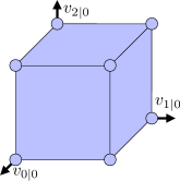
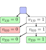
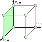
Time $\tau=1$

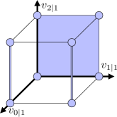
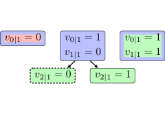
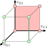
Figure 1: Illustration of the synthetic Example 1. The first row describes the cold-started solution of the MIQP at time $\tau=0$, reporting the initial cover $\mathscr{V}_{0}^{0}$, the B&B tree, and the final cover $\mathscr{V}_{0}^{*}$. In the second row we depict the same elements for the warm-started MIQP at time $\tau=1$. The optimal binary actions for $\tau=0$ and $\tau=1$ are $v_{0}:=v_{0\mid 0}^{*}=1$ and $v_{1}:=v_{0\mid 1}^{*}=1$, respectively. These determine which leaves are kept (green) and which are discarded (red) during the construction of the subsequent initial covers. Root nodes are colored in light blue, and leaves associated with the optimal solutions have a dashed contour. The sets in the initial and final covers are colored and contoured in accordance with the B&B tree.

We consider a toy problem where the system has a single binary variable $m_{u}=1$ and the horizon of the controller is $T=3$. At time $\tau=0$ the B&B algorithm is initialized with the trivial cover $\mathscr{V}_{0}^{0}=\{[(0,0,0),(1,1,1)]\}$ (top-left cell in Figure 1). Assuming the $\varepsilon$-optimal binary assignment to be $(v_{0\mid 0}^{*},v_{1\mid 0}^{*},v_{2\mid 0}^{*})=(1,1,0)$, the B&B tree is shown in the top-center cell. The root node (light blue) consists in the solution of the subproblem $\mathbf{P}_{0}([(0,0,0),(1,1,1)])$, whereas the optimal leaf node has a dashed contour and is associated with $\mathbf{P}_{0}([(1,1,0),(1,1,0)])$. The final cover for $\mathbf{P}_{0}$ is

$$\mathscr{V}_{0}^{*}=\{[(0,0,0),(1,0,1)],[(0,1,0),(0,1,1)],\\ [(1,1,0),(1,1,0)],[(1,1,1),(1,1,1)]\}$$ (9)

and is depicted in the top-right cell.

Among all the leaves at time $\tau=0$, the only one that does not verify condition (7), for $v_{0}:=v_{0\mid 0}^{*}=1$, is colored in red and represents problem $\mathbf{P}_{0}([(0,1,0),(0,1,1)])$. This interval is hence dropped in the construction of the initial cover $\mathscr{V}_{1}^{0}$, while all the other leaves (green) are shifted in time and added to $\mathscr{V}_{1}^{0}$. (Note that the sets in the final cover are colored and contoured to match the B&B tree.) After the time shift (8) of the bounds, we get the initial cover for $\mathbf{P}_{1}$:

$$\mathscr{V}_{1}^{0}=\{[(0,0,0),(0,1,1)],[(1,0,0),(1,0,1)],\\ [(1,1,0),(1,1,1)]\},$$ (10)

which is depicted in the bottom-left cell in Figure 1.

The B&B tree at time $\tau=1$ (bottom-center cell) has three root nodes, one per set in $\mathscr{V}_{1}^{0}$. Its $\varepsilon$-optimal solution (dashed leaf) is $(v_{0\mid 1}^{*},v_{1\mid 1}^{*},v_{2\mid 1}^{*})=(1,0,0)$, and leads to the final cover $\mathscr{V}_{1}^{*}$ depicted in the bottom-right cell. The same procedure is then applied again to select the leaves for the construction of $\mathscr{V}_{2}^{0}$: green leaves are kept, the red leaf is dropped. ∎

V Propagation of Subproblem Lower Bounds

The second step in the construction of our warm start is to equip each set in the cover $\mathscr{V}_{1}^{0}$ with a lower bound for the associated minimization problem. The strategy we adopt is to construct a dual-feasible solution for each of these QPs.

From the solution of $\mathbf{P}_{0}$ via B&B we retrieve the terminal cover $\mathscr{V}_{0}^{*}$ and, for each interval $\mathcal{V}_{0}$ in it, we have a feasible solution for the dual subproblem $\mathbf{D}_{0}(\mathcal{V}_{0})$. This can be optimal or just feasible, or even a certificate of infeasibility in case we proved that $\theta_{0}(\mathcal{V}_{0})=\infty$. By means of the construction presented in Section IV, a set $\mathcal{V}_{0}$ (if not discarded) is associated with an element $\mathcal{V}_{1}$ of the initial cover $\mathscr{V}_{1}^{0}$. The following lemma shows how a solution of $\mathbf{D}_{0}(\mathcal{V}_{0})$ can be shifted in time to comply with the constraints of $\mathbf{D}_{1}(\mathcal{V}_{1})$.

Lemma 1.

Let $\{\lambda_{t\mid 0},\rho_{t\mid 0}\}_{t=0}^{T}$ and $\{\mu_{t\mid 0},\underaccent{\bar{}}{\nu}_{t\mid 0},\bar{\nu}_{t\mid 0},\sigma_{t\mid 0}\}_{t=0}^{T-1}$ be feasible multipliers for $\mathbf{D}_{0}(\mathcal{V}_{0})$. The following set of multipliers is feasible for $\mathbf{D}_{1}(\mathcal{V}_{1})$:

• $(\lambda_{t\mid 1},\rho_{t\mid 1}):=(\lambda_{t+1\mid 0},\rho_{t+1\mid 0})$ for $t=0,\ldots,T-1$,

• $(\lambda_{T\mid 1},\rho_{T\mid 1}):=0$,

• $(\mu_{t\mid 1},\underaccent{\bar{}}{\nu}_{t\mid 1},\bar{\nu}_{t\mid 1},\sigma_{t\mid 1}):=(\mu_{t+1\mid 0},\underaccent{\bar{}}{\nu}_{t+1\mid 0},\bar{\nu}_{t+1\mid 0},\sigma_{t+1\mid 0})$ for $t=0,\ldots,T-2$,

• $(\mu_{T-1\mid 1},\underaccent{\bar{}}{\nu}_{T-1\mid 1},\bar{\nu}_{T-1\mid 1},\sigma_{T-1\mid 1}):=0$.

Proof.

We substitute the candidate solution in the constraints of $\mathbf{D}_{1}(\mathcal{V}_{1})$. From (6b) we obtain $Q^{\prime}\rho_{t+1\mid 0}+\lambda_{t+1\mid 0}-A^{\prime}\lambda_{t+2\mid 0}+F^{\prime}\mu_{t+1\mid 0}=0$ for $t=0,\ldots,T-2$, and $Q^{\prime}\rho_{T\mid 0}+\lambda_{T\mid 0}=0$. These constraints are verified by feasibility of the multipliers at time $\tau=0$. The constraint (6c) holds trivially, as well as condition (6d) for $t=T-1$. For $t=0,\ldots,T-2$, the constraint (6d) becomes $R^{\prime}\sigma_{t+1\mid 0}-B^{\prime}\lambda_{t+2\mid 0}+G^{\prime}\mu_{t+1\mid 0}+V^{\prime}(\bar{\nu}_{t+1\mid 0}-\underaccent{\bar{}}{\nu}_{t+1\mid 0})=0$, which holds again by feasibility of the multipliers at time $\tau=0$. Nonnegativity of $\mu_{t\mid 1}$, $\underaccent{\bar{}}{\nu}_{t\mid 1}$, and $\bar{\nu}_{t\mid 1}$ is ensured by construction. ∎

Lemma 1 has several implications. Given a set in $\mathscr{V}_{0}^{*}$ and a dual-feasible solution for the associated QP, we can now equip with feasible multipliers, and hence a lower bound, the related set in $\mathscr{V}_{1}^{0}$. Since we just assumed feasibility of the multipliers at time step $\tau=0$, Lemma 1 applies even if, as it is frequently the case, $\mathbf{D}_{0}(\mathcal{V}_{0})$ is not solved to optimality. Similarly, if the bound we generate for $\mathbf{D}_{1}(\mathcal{V}_{1})$ is tight enough to prevent its solution within the B&B at time $\tau=1$, the synthesized dual variables can in turn be propagated to bound the optimal value of a subproblem at time $\tau=2$. On the other hand, if solving $\mathbf{D}_{1}(\mathcal{V}_{1})$ turns out to be necessary, we can still use the multipliers from Lemma 1 to warm start this QP solve. Clearly, as we shift a dual solution across time steps, the tightness of the implied bound will gradually decay, and a few iterations of the QP solver will eventually be required. However, this is inevitable: the problem on which we are inferring a bound is increasingly different from the one we actually solved. Finally, note that Lemma 1 holds despite any potential model error $e_{0}$: the current state $x_{1}=Ax_{0}+Bu_{0}+e_{0}$ appears in the dual problem $\mathbf{D}_{1}(\mathcal{V}_{1})$ as a cost coefficient and, as such, it does not affect dual feasibility.

The following theorem concerns the tightness of the lower bounds we construct via Lemma 1.

Theorem 1.

Let $\{\lambda_{t\mid 0},\rho_{t\mid 0}\}_{t=0}^{T}$ and $\{\mu_{t\mid 0},\underaccent{\bar{}}{\nu}_{t\mid 0},\bar{\nu}_{t\mid 0},\sigma_{t\mid 0}\}_{t=0}^{T-1}$ be feasible multipliers for $\mathbf{D}_{0}(\mathcal{V}_{0})$ with cost $\underaccent{\bar{}}{\theta}_{0}(\mathcal{V}_{0})$. Define

$$\pi_{1}:=\ -|Qx_{0}|^{2}-|Ru_{0}|^{2},$$ (11a)

$$\pi_{2}:=\ |\rho_{0\mid 0}/2-Qx_{0}|^{2}+|\sigma_{0\mid 0}/2-Ru_{0}|^{2},$$ (11b)

$$\pi_{3}:=\ (h-Fx_{0}-Gu_{0})^{\prime}\mu_{0\mid 0}+(v_{0}-\underaccent{\bar{}}{v}_{0\mid 0})^{\prime}\underaccent{\bar{}}{\nu}_{0\mid 0}$$

$$+(\bar{v}_{0\mid 0}-v_{0})^{\prime}\bar{\nu}_{0\mid 0},$$ (11c)

$$\pi_{4}:=\ -e_{0}^{\prime}\lambda_{1\mid 0}.$$ (11d)

The following is a lower bound on $\theta_{1}(\mathcal{V}_{1})$:

$$\underaccent{\bar{}}{\theta}_{1}(\mathcal{V}_{1}):=\underaccent{\bar{}}{\theta}_{0}(\mathcal{V}_{0})+\sum_{i=1}^{4}\pi_{i}.$$ (12)

Proof.

See Appendix C. ∎

Despite the many terms, Theorem 1 is very informative, and an inspection of the expressions in (11) reveals the following. We recall that, since we are working with lower bounds, we would like these terms to be positive.

• This term represents the MIQP stage cost for $\tau=0$. It is nonpositive, but this was expected: standard MPC arguments show that the value function $\theta_{\tau}$ can actually decrease at this rate (in the absence of disturbances and as the horizon $T$ tends to infinity).

• Recalling the stationarity conditions (29) from Appendix B, we notice that this nonnegative term vanishes in case the multipliers $\rho_{0\mid 0}$, $\sigma_{0\mid 0}$ are optimal for $\mathbf{D}_{0}(\mathcal{V}_{0})$, and the control action $u_{0}$ (injected in the system at time $\tau=0$) is optimal for the subproblem $\mathbf{P}_{0}(\mathcal{V}_{0})$.

• Because of the feasibility of $u_{0}$, the condition $\underaccent{\bar{}}{v}_{0\mid 0}\leq v_{0}\leq\bar{v}_{0\mid 0}$ imposed in the construction of $\mathscr{V}_{1}^{0}$, and the nonnegativity of $\mu_{0\mid 0}$, $\underaccent{\bar{}}{\nu}_{0\mid 0}$, $\bar{\nu}_{0\mid 0}$, this term is nonnegative. If these multipliers are optimal for $\mathbf{D}_{0}(\mathcal{V}_{0})$ and $u_{0}$ is optimal for $\mathbf{P}_{0}(\mathcal{V}_{0})$, this term vanishes by complementary slackness.

• This term is linear in the model error $e_{0}$. It is null in case of a perfect model, while it can have either sign in case of discrepancies.

Notably, for a perfect model $e_{0}=0$, the difference $\underaccent{\bar{}}{\theta}_{1}(\mathcal{V}_{1})-\underaccent{\bar{}}{\theta}_{0}(\mathcal{V}_{0})$ is bounded below by $\pi_{1}$, which does not depend on the particular pair $\mathbf{P}_{0}(\mathcal{V}_{0})$, $\mathbf{P}_{1}(\mathcal{V}_{1})$ of subproblems we are considering.

Together with a better insight into the tightness of the bounds we propagate, Theorem 1 also gives us a sufficient condition for the infeasibility of $\mathbf{P}_{1}(\mathcal{V}_{1})$. The next corollary shows how a certificate of infeasibility for $\mathbf{P}_{0}(\mathcal{V}_{0})$ can be transformed into a certificate for $\mathbf{P}_{1}(\mathcal{V}_{1})$.

Corollary 1.

Let $\{\lambda_{t\mid 0},\rho_{t\mid 0}\}_{t=0}^{T}$ and $\{\mu_{t\mid 0},\underaccent{\bar{}}{\nu}_{t\mid 0},\bar{\nu}_{t\mid 0},\sigma_{t\mid 0}\}_{t=0}^{T-1}$ be a certificate of infeasibility for $\mathbf{P}_{0}(\mathcal{V}_{0})$ with dual objective $\underaccent{\bar{}}{\theta}_{0}(\mathcal{V}_{0})$. Then, the set of dual variables defined in Lemma 1 is a certificate of infeasibility for $\mathbf{P}_{1}(\mathcal{V}_{1})$ as long as $e_{0}$ lies in the open halfspace

$$\lambda_{1\mid 0}^{\prime}e_{0}<\underaccent{\bar{}}{\theta}_{0}(\mathcal{V}_{0})+\pi_{3}.$$ (13)

Moreover, this inequality is always verified if $e_{0}=0$.

Proof.

We check the definition of a certificate of infeasibility from Section III-B. In Lemma 1 we have shown dual feasibility of these multipliers, and, by construction, we have $\rho_{t\mid 1}=0$ and $\sigma_{t\mid 1}=0$ for all $t$. We are then left to verify positivity of their dual cost $\underaccent{\bar{}}{\theta}_{1}(\mathcal{V}_{1})$. Using Theorem 1, we have $\pi_{1}+\pi_{2}=0$ and $\underaccent{\bar{}}{\theta}_{1}(\mathcal{V}_{1})=\underaccent{\bar{}}{\theta}_{0}(\mathcal{V}_{0})+\pi_{3}+\pi_{4}$, which leads to (13). Finally, since $\pi_{3}\geq 0$ and $\underaccent{\bar{}}{\theta}_{0}(\mathcal{V}_{0})>0$, $e_{0}=0$ always satisfies this inequality. ∎

Corollary 1 completes the tools we need to equip with lower bounds the initial cover $\mathscr{V}_{1}^{0}$. For any set $\mathcal{V}_{0}$ in $\mathscr{V}_{0}^{*}$ that corresponds to an infeasible QP, we can now associate a halfspace in the error space inside which the descendant problem $\mathbf{P}_{1}(\mathcal{V}_{1})$ will also be infeasible. Moreover, since the set defined by (13) contains the origin, in case of an exact MLD model, infeasibility of the descendant subproblem is guaranteed. As for Lemma 1, this process can be iterated and the same certificate propagated across multiple time steps.

Except for the computation of $\pi_{4}$, which only amounts to $|\mathscr{V}_{1}^{0}|$ scalar products in $\mathbb{R}^{n_{x}}$, all the steps in this section can be performed before the measurement of the next state $x_{1}$, leading to a negligible time delay in the solution of $\mathbf{P}_{1}$.

VI Propagation of an Upper Bound

The last element we need to warm start the solution of the MIQP $\mathbf{P}_{1}$ is an upper bound $\bar{\theta}_{1}^{0}$ on its optimal value. The natural way to address this problem is to shift the $\varepsilon$-optimal solution of $\mathbf{P}_{0}$ and synthesize a feasible solution for $\mathbf{P}_{1}$.

The issue of persistent feasibility has been widely studied in hybrid MPC (see [44, Section 3.5] or [27, Sections 12.3.1 and 17.8.1]). The standard approach consists in designing the MPC problem so that the terminal state $x_{T\mid\tau}$ lies in a control-invariant set $\mathcal{X}$ which contains the origin. More specifically, for all $x$ in $\mathcal{X}$ there must exist a control action $u\in\mathbb{R}^{n_{u}}\times\{0,1\}^{m_{u}}$ such that $(x,u)\in\mathcal{D}$ and $Ax+Bu\in\mathcal{X}$. When this is the case, the existence of an input $u_{T-1\mid 1}$, such that the control sequence $\{u_{1\mid 0}^{*},\ldots,u_{T-1\mid 0}^{*},u_{T-1\mid 1}\}$ is feasible for $\mathbf{P}_{1}$, is guaranteed. The computation of the upper bound $\bar{\theta}_{1}^{0}$ then amounts, in the worst case, to the solution of $2^{m_{u}}$ QPs.

There are two standard ways to fulfill the requirement $x_{T\mid\tau}\in\mathcal{X}$, both with well-known pros and cons [1]. The first is to make the MPC horizon $T$ long enough so that the invariance condition is spontaneously verified. The second is to enforce it explicitly as a terminal constraint in our MIQP. While the first approach complies with the problem formulation from (2), as already mentioned, the implementation of the second requires a more versatile problem statement which we will consider in Section VIII.

In contrast to Section V, here we can only generate upper bounds for a perfect model $e_{0}=0$. A potential workaround would be to consider a robust version of problem (2), where persistent feasibility is guaranteed despite disturbances of bounded magnitude. This, however, would lead to substantially harder optimization problems (see, e.g., [45] or [44, Chapter 5]).

VII Asymptotic Analysis

We proceed in the analysis of the warm-start algorithm studying its asymptotic behavior as the horizon $T$ grows. In doing so, we assume the MLD model to be perfect ($e_{0}=0$).

In order to link the lower bounds from Theorem 1 with the decrease rate of the cost to go $\theta_{\tau}$, we take advantage of the following observation.

Lemma 2.

Consider a perfect MLD model (1). For any control action $u_{0}\in\mathbb{R}^{n_{u}}\times\{0,1\}^{m_{u}}$ applied to the system at time $\tau=0$ such that $(x_{0},u_{0})\in\mathcal{D}$, we have $\theta_{1}\geq\theta_{0}-|Qx_{0}|^{2}-|Ru_{0}|^{2}$.

Proof.

Let $\underaccent{\bar{}}{\theta}_{1}\in\mathbb{R}_{\geq 0}\cup\{\infty\}$ be the optimal value of the problem we obtain by shortening the horizon of $\mathbf{P}_{1}$ by one time step. Clearly, $\underaccent{\bar{}}{\theta}_{1}\leq\theta_{1}$. On the other hand, we must also have $\theta_{0}\leq\underaccent{\bar{}}{\theta}_{1}+|Qx_{0}|^{2}+|Ru_{0}|^{2}$. In fact, if this was not true, prepending $u_{0}$ to the optimal controls from the shortened $\mathbf{P}_{1}$ we would get a solution for $\mathbf{P}_{0}$ with cost lower than $\theta_{0}$, a contradiction. The lemma follows by chaining these two inequalities. ∎

The following theorems can be seen as “sanity checks” for the asymptotic behavior of the warm-start algorithm as $T$ tends to infinity. More specifically, let $\mathcal{V}_{0}^{*}\in\mathscr{V}_{0}^{*}$ be the set which contains the $\varepsilon$-optimal binary assignment found via B&B at time $\tau=0$, and denote with $\mathcal{V}_{1}^{*}$ its descendant through the procedure presented in Section IV. We show that $\mathcal{V}_{1}^{*}$ must contain a binary assignment which is $\varepsilon$-optimal for $\mathbf{P}_{1}$. Moreover, $\varepsilon$-optimality of this assignment is directly proved by the initial cover $\mathscr{V}_{1}^{0}$ from Section IV, equipped with the lower bounds from Theorem 1. This formalizes the intuition that, as the horizon grows and the MPC policy tends to be stationary, the warm-started B&B should only reoptimize the final stage of the trajectory.

Theorem 2.

Consider a perfect MLD model (1), and let the horizon $T$ go to infinity. The set $\mathcal{V}_{1}^{*}$ contains a binary-feasible assignment for $\mathbf{P}_{1}$ with cost $\theta_{1}^{*}\leq\theta_{1}+\varepsilon$.

Proof.

As $T$ goes to infinity, the terminal state $x_{T\mid 0}$ of any feasible solution for $\mathbf{P}_{0}$ must lie in a control-invariant set $\mathcal{X}$ within which cost is not accumulated. More precisely, $\mathcal{X}\subseteq\mathrm{ker}(Q)$ and for all $x\in\mathcal{X}$ there must exist a $u\in\mathbb{R}^{n_{u}}\times\{0,1\}^{m_{u}}$ such that $Ru=0$, $(x,u)\in\mathcal{D}$, and $Ax+Bu\in\mathcal{X}$. Thus, the $\varepsilon$-optimal solution of $\mathbf{P}_{0}$ with cost $\theta_{0}^{*}\leq\theta_{0}+\varepsilon$ can be shifted in time to synthesize a feasible solution for $\mathbf{P}_{1}$ with cost $\theta_{1}^{*}:=\theta_{0}^{*}-|Qx_{0}|^{2}-|Ru_{0}|^{2}\leq\theta_{0}+\varepsilon-|Qx_{0}|^{2}-|Ru_{0}|^{2}$. The binaries of the synthesized solution belong to $\mathcal{V}_{1}^{*}$ and, using Lemma 2, we get $\theta_{1}^{*}\leq\theta_{1}+\varepsilon$. ∎

Theorem 3.

Let the assumptions of Theorem 2 hold, and let $\theta_{1}^{*}$ be defined as in its proof. The bounds from Theorem 1 verify the condition $\underaccent{\bar{}}{\theta}_{1}(\mathcal{V}_{1})\geq\theta_{1}^{*}-\varepsilon$ for all $\mathcal{V}_{1}$ in $\mathscr{V}_{1}^{0}$.

Proof.

Consider a generic set $\mathcal{V}_{1}\in\mathscr{V}_{1}^{0}$ and its ancestor $\mathcal{V}_{0}\in\mathscr{V}_{0}^{*}$. Since $\pi_{2}$ and $\pi_{3}$ from Theorem 1 are nonnegative and $\pi_{4}=0$ by assumption, we have $\underaccent{\bar{}}{\theta}_{1}(\mathcal{V}_{1})\geq\underaccent{\bar{}}{\theta}_{0}(\mathcal{V}_{0})+\pi_{1}$. By convergence of the B&B at time $\tau=0$, we have $\underaccent{\bar{}}{\theta}_{0}(\mathcal{V}_{0})\geq\theta_{0}^{*}-\varepsilon$ for all $\mathcal{V}_{0}$ in $\mathscr{V}_{0}^{*}$ (see condition (5)). These imply $\theta_{1}^{*}:=\theta_{0}^{*}+\pi_{1}\leq\underaccent{\bar{}}{\theta}_{0}(\mathcal{V}_{0})+\varepsilon+\pi_{1}\leq\underaccent{\bar{}}{\theta}_{1}(\mathcal{V}_{1})+\varepsilon$ for all $\mathcal{V}_{1}$ in $\mathscr{V}_{1}^{0}$. ∎

VIII Terminal Penalties and Constraints

The main limitation of problem statement (2) is its incompatibility with terminal penalties and constraints. In this section, we extend the warm-start algorithm to cost functions and constraints which vary with the relative time $t$. First, we consider time-dependent weight matrices $Q_{t}$ and $R_{t}$ in the objective (2a). Once again, we make no assumptions on the rank of these matrices. Then we replace the constraint set $\mathcal{D}$ in (2d) with the time-dependent polyhedron $\mathcal{D}_{t}:=\{(x,u)\mid F_{t}x+G_{t}u\leq h_{t}\}$, which is assumed to contain the origin and to be contained in $\mathcal{D}$. In this wider framework, terminal penalties can be enforced by modulating the value of $Q_{T}$ and terminal constraints via a suitable definition of $\mathcal{D}_{T-1}$. Note that, a polyhedral constraint on $x_{T\mid\tau}$ maps to a polyhedral constraint on $(x_{T-1\mid\tau},u_{T-1\mid\tau})$ via the dynamics (2c).

Clearly, in these more general settings, the asymptotic analysis from Section VII, which was based on the limiting stationarity of the MPC policy, might not hold. In addition, in case of wild variations of the problem data $Q_{t}$, $R_{t}$, $\mathcal{D}_{t}$ with the relative time $t$, we expect a warm start generated by shifting the previous solution to be fairly ineffective. However, as we show in this section, our algorithm deals with these issues very transparently, propagating dual bounds that are parametric in the variations of these problem data.

VIII-A Stage Cost Varying with the Relative Time

We start discussing the implications of time-dependent weight matrices $Q_{t}$ and $R_{t}$. We do so under the following assumption which, in words, requires the weight matrices for time $t+1$ to penalize only the state and input entries that are also penalized at stage $t$.

Assumption 1.

The row space of $Q_{t}$ contains the row space of $Q_{t+1}$ for $t=0,\ldots,T-1$, and the row space of $R_{t}$ contains the row space of $R_{t+1}$ for $t=0,\ldots,T-2$.

Out of the three components of our warm-start procedure, only the propagation of lower bounds (discussed in Section V) is affected by the time dependency of $Q_{t}$ and $R_{t}$. Here, we extend this component starting from Lemma 1, and then considering Theorem 1 and Corollary 1.

VIII-A1 Modifications to Lemma 1

Following the steps from Appendix B, the dual problem (6) can be easily adjusted to comply with time-varying weights. Constraints (6b) and (6d) require the substitution of $Q$ and $R$ with $Q_{t}$ and $R_{t}$, respectively. Constraint (6c) now depends on $Q_{T}$ instead of $Q$. This modification breaks the shifting procedure presented in Lemma 1. To restore it, we redefine $\rho_{t\mid 1}$ for $t=0,\ldots,T-1$ and $\sigma_{t\mid 1}$ for $t=0,\ldots,T-2$, explicitly enforcing the conditions $Q_{t}^{\prime}\rho_{t\mid 1}=Q_{t+1}^{\prime}\rho_{t+1\mid 0}$ and $R_{t}^{\prime}\sigma_{t\mid 1}=R_{t+1}^{\prime}\sigma_{t+1\mid 0}$. Furthermore, among all the solutions of these linear systems, we select the ones that maximize the lower bound $\underaccent{\bar{}}{\theta}_{1}(\mathcal{V}_{1})$ or, equivalently, minimize $|\rho_{t\mid 1}|^{2}$ and $|\sigma_{t\mid 1}|^{2}$. This choice leads to two quadratic optimization problems, which, under Assumption 1, are always feasible and admit closed-form solution:

$$\rho_{t\mid 1}:=(Q_{t}^{\prime})^{+}Q_{t+1}^{\prime}\rho_{t+1\mid 0}, t=0,\ldots,T-1,$$ (14a)

$$\sigma_{t\mid 1}:=(R_{t}^{\prime})^{+}R_{t+1}^{\prime}\sigma_{t+1\mid 0}, t=0,\ldots,T-2.$$ (14b)

VIII-A2 Modifications to Theorem 1 and Corollary 1

Theorem 1 can be adapted to the time dependency of $Q_{t}$ and $R_{t}$ by retracing the steps from Appendix C. The definitions in (11) are still valid, provided that we substitute the matrices $Q$ and $R$ with $Q_{0}$ and $R_{0}$. The lower bound $\underaccent{\bar{}}{\theta}_{1}(\mathcal{V}_{1})$ from (12) requires the addition of two terms:

$$\pi_{5}:= \frac{1}{4}\sum_{t=0}^{T-1}(|\rho_{t+1\mid 0}|^{2}-|\rho_{t\mid 1}|^{2}),$$ (15a)

$$\pi_{6}:= \frac{1}{4}\sum_{t=0}^{T-2}(|\sigma_{t+1\mid 0}|^{2}-|\sigma_{t\mid 1}|^{2}),$$ (15b)

which do not cancel out anymore. In the following propositions we analyze the sign of $\pi_{5}$ and $\pi_{6}$.

Proposition 2.

A necessary and sufficient condition for $\pi_{5}$ to be nonnegative for all $\rho_{1\mid 0},\ldots,\rho_{T\mid 0}$ is $\|Q_{t+1}Q_{t}^{+}\|\leq 1$ for $t=0,\ldots,T-1$.

Proof.

By definition of the operator norm, we have $|\rho_{t\mid 1}|\leq\|Q_{t+1}Q_{t}^{+}\||\rho_{t+1\mid 0}|$. Sufficiency follows from

$$\pi_{5}\geq\frac{1}{4}\sum_{t=0}^{T-1}(1-\|Q_{t+1}Q_{t}^{+}\|^{2})|\rho_{t+1\mid 0}|^{2}.$$ (16)

For the other direction, note that equality in (16) can always be attained for some nonzero $\rho_{1\mid 0},\ldots,\rho_{T\mid 0}$. ∎

Proposition 3.

A necessary and sufficient condition for $\pi_{6}$ to be nonnegative for all $\sigma_{1\mid 0},\ldots,\sigma_{T-1\mid 0}$ is $\|R_{t+1}R_{t}^{+}\|\leq 1$ for $t=0,\ldots,T-2$.

Proof.

Analogous to the proof of Proposition 2. ∎

These propositions suggest that, when the magnitude of the weight matrices $Q_{t}$ and $R_{t}$ increases with the relative time $t$, the terms $\pi_{5}$ and $\pi_{6}$ might be negative. On the other hand, when the weights decrease with $t$ (or when they are constant as in Theorem 1), $\pi_{5}$ and $\pi_{6}$ tend to tighten the bounds $\underaccent{\bar{}}{\theta}_{1}(\mathcal{V}_{1})$. Unfortunately, terminal penalties fall under the first scenario, but this was to be expected: since the final state of $\mathbf{P}_{1}(\mathcal{V}_{1})$ is likely to be smaller in magnitude than the one of $\mathbf{P}_{0}(\mathcal{V}_{0})$, when increasing $Q_{T}$, we expect the difference $\theta_{1}(\mathcal{V}_{1})-\theta_{0}(\mathcal{V}_{0})$ to decrease.

Finally, Corollary 1 remains unchanged as well as inequality (13). In fact, if the multipliers we are given for $\tau=0$ certify infeasibility of $\mathbf{P}_{0}(\mathcal{V}_{0})$, then $\rho_{t\mid 0}=0$ and $\sigma_{t\mid 0}=0$ for all $t$. Using (14), we get $\rho_{t\mid 1}=0$ and $\sigma_{t\mid 1}=0$, and the additional terms $\pi_{5}$ and $\pi_{6}$ from (15) vanish.

VIII-B Constraint Set Varying with the Relative Time

We discuss time-dependent constraints under the following assumption, which holds, for example, in the common case of bounded constraint sets $\mathcal{D}_{t}$.

Assumption 2.

The conic hull of the rows of $[F_{t}\ G_{t}]$ contains the conic hull of the rows of $[F_{t+1}\ G_{t+1}]$ for $t=0,\ldots,T-2$.

Out of the three warm start components, the time dependency of $\mathcal{D}_{t}$ affects mainly the propagation of lower bounds. The construction of the initial cover is unchanged and, for the upper-bound propagation, in order to preserve persistent feasibility, we only require $\mathcal{D}_{t+1}\subseteq\mathcal{D}_{t}$ for $t=0,\ldots,T-2$. Once again we discuss the adaptations of Lemma 1 and of Theorem 1 and Corollary 1 separately.

VIII-B1 Modifications to Lemma 1

In case of time-dependent constraints $\mathcal{D}_{t}$, the matrices $F$, $G$, and $h$ in the dual problem (6) must have the subscript $t$. This modification makes the arguments from Lemma 1 untrue. The ideal fix would be to define $\mu_{t\mid 1}$ through the Linear Program (LP)

$$\min\ h_{t}^{\prime}\mu_{t\mid 1}$$ (17a)

$$\mathrm{s.t.}\ F_{t}^{\prime}\mu_{t\mid 1}=F_{t+1}^{\prime}\mu_{t+1\mid 0},$$ (17b)

$$G_{t}^{\prime}\mu_{t\mid 1}=G_{t+1}^{\prime}\mu_{t+1\mid 0},$$ (17c)

$$\mu_{t\mid 1}\geq 0,$$ (17d)

for $t=0,\ldots,T-2$. These LPs would maximize the lower bounds $\underaccent{\bar{}}{\theta}_{1}(\mathcal{V}_{1})$ and, under Assumption 2, they would always be feasible. However, keeping in mind that our ultimate goal is to bound the optimal value of a QP, this definition of $\mu_{t\mid 1}$ is clearly impractical. Nonetheless, finding a good approximate solution to these LPs turns out to be relatively simple.

Let $\mu_{t\mid 1}^{*}(\mu_{t+1\mid 0})$ be the parametric minimizer of problem (17). We define $M_{t\mid 1}$ as the matrix whose $i$th column is $\mu_{t\mid 1}^{*}(\epsilon_{i})$, with $\epsilon_{i}$ $i$th element of the standard basis. Note that $M_{t\mid 1}$ can be easily computed offline by solving one LP per entry in $\mu_{t+1\mid 0}$ (i.e., per facet of the polyhedron $\mathcal{D}_{t+1}$).

Proposition 4.

The multiplier $\mu_{t\mid 1}:=M_{t\mid 1}\mu_{t+1\mid 0}$ is feasible for the LP (17).

Proof.

Since $\mu_{t+1\mid 0}$ and $\mu_{t\mid 1}^{*}(\epsilon_{i})$ are nonnegative, so is $\mu_{t\mid 1}$. By feasibility of $\mu_{t\mid 1}^{*}$, we have $F_{t}^{\prime}M_{t\mid 1}=F_{t+1}^{\prime}$ and $G_{t}^{\prime}M_{t\mid 1}=G_{t+1}^{\prime}$, which imply conditions (17b) and (17c). ∎

Coming back to the primal side, the LP (17) has a clear geometrical meaning. Its dual reads

$$\max\ \mu_{t+1\mid 0}^{\prime}(F_{t+1}x_{t\mid 1}+G_{t+1}u_{t\mid 1})$$ (18a)

$$\mathrm{s.t.}\ F_{t}x_{t\mid 1}+G_{t}u_{t\mid 1}\leq h_{t},$$ (18b)

where the optimization variables are the state $x_{t\mid 1}$ and the input $u_{t\mid 1}$. For $\mu_{t+1\mid 0}=\epsilon_{i}$, the LP (18) is illustrated in Figure 2, and allows to determine whether the polyhedron $\mathcal{D}_{t}$ lies within the halfspace delimited by the $i$th facet of $\mathcal{D}_{t+1}$. In words, this optimization finds the point in $\mathcal{D}_{t}$ which violates most the $i$th inequality defining $\mathcal{D}_{t+1}$. Containment is certified in case the maximum of this problem, which corresponds to $h_{t}^{\prime}\mu_{t\mid 1}^{*}(\epsilon_{i})$ by strong duality, is lower or equal to the $i$th entry of $h_{t+1}$.

If the polyhedron $\mathcal{D}_{t}$ is entirely contained in $\mathcal{D}_{t+1}$, the above observation applies for all $i$, and we have $h_{t}^{\prime}M_{t\mid 1}\leq h_{t+1}^{\prime}$. This inequality can in turn be used to bound the cost of $\mu_{t\mid 1}$ from Proposition 4, leading to

$$h_{t}^{\prime}\mu_{t\mid 1}=h_{t}^{\prime}M_{t\mid 1}\mu_{t+1\mid 0}\leq h_{t+1}^{\prime}\mu_{t+1\mid 0}.$$ (19)

We will take advantage of this bound in the revision of Theorem 1.

Figure 2: Geometrical interpretation of the LP (18) as a containment problem. The color gradient in $\mathcal{D}_{t}$ symbolizes the objective function. For $\mu_{t+1\mid 0}=\epsilon_{i}$, problem (18) returns the point (blue star) in $\mathcal{D}_{t}$ which violates most the $i$th constraint (facet) of $\mathcal{D}_{t+1}$. Depending on whether the polyhedron $\mathcal{D}_{t}$ lies inside the $i$th facet of $\mathcal{D}_{t+1}$, the optimal value of (17), and of its dual (18), is lower (left image) or greater (right image) than the $i$th entry of $h_{t+1}$.

VIII-B2 Modifications to Theorem 1 and Corollary 1

When the sets $\mathcal{D}_{t}$ vary with the relative time $t$, the matrices $F$, $G$, and $h$ in the definition of $\pi_{3}$ must be substituted with $F_{0}$, $G_{0}$, and $h_{0}$. The lower bounds $\underaccent{\bar{}}{\theta}_{1}(\mathcal{V}_{1})$ from Theorem 1 require the additional term

$$\pi_{7}:=\sum_{t=0}^{T-2}(h^{\prime}_{t+1}\mu_{t+1\mid 0}-h^{\prime}_{t}\mu_{t\mid 1}).$$ (20)

The observation made in (19) suggests the following sufficient condition for the nonnegativity of $\pi_{7}$.

Proposition 5.

Let $\mu_{t\mid 1}$ be defined as in Proposition 4. If $\mathcal{D}_{t}\subseteq\mathcal{D}_{t+1}$ for $t=0,\ldots,T-2$, then $\pi_{7}\geq 0$. Additionally, if $\mathcal{D}_{t}=\mathcal{D}_{t+1}$, we have $\pi_{7}=0$.

Proof.

The nonnegativity condition follows from (19). In case $\mathcal{D}_{t}=\mathcal{D}_{t+1}$, the optimal value of (17) for $\mu_{t+1\mid 0}=\epsilon_{i}$ coincides with the $i$th entry of $h_{t+1}$, for all $i$. Therefore, we have $h^{\prime}_{t}M_{t\mid 1}=h_{t+1}^{\prime}$, the relation in (19) holds with the equality, and $\pi_{7}$ vanishes. ∎

Even if the condition $\mathcal{D}_{t}\subseteq\mathcal{D}_{t+1}$ is frequently violated in practice (terminal constraints, for example, lead to $\mathcal{D}_{T-2}\supset\mathcal{D}_{T-1}$), Proposition 5 shows that the definition of $\mu_{t\mid 1}$ from Proposition 4 is a natural generalization of the shifting process from Lemma 1. In fact, when the constraint sets $\mathcal{D}_{t}$ are actually constant with the relative time $t$, the two approaches lead to the same lower bounds $\underaccent{\bar{}}{\theta}_{1}(\mathcal{V}_{1})$.

With this choice of the multipliers $\mu_{t\mid 1}$, the statement of Corollary 1 is still valid, provided that we add $\pi_{7}$ to the right-hand side of (13). Furthermore, if $\mathcal{D}_{t}\subseteq\mathcal{D}_{t+1}$ for all $t$, the origin $e_{0}=0$ is still guaranteed to verify condition (13). On the contrary, if the constraint sets shrink with the relative time $t$, it might be the case that an infeasible subproblem at time $\tau=0$ has a feasible descendant at $\tau=1$, even in the nominal case $e_{0}=0$.

IX Numerical Study

We test the proposed warm-start algorithm on a numerical example. We consider a linearized version of the cart-pole system depicted in Figure 3: the goal is to regulate the cart in the center of the two walls with the pole in the upright position. To accomplish this task, we can apply a force directly on the cart and exploit contact forces that arise when the tip of the pole collides with the walls. This regulation problem has been used to benchmark control-through-contact algorithms in [18, 46], and its moderate size allows an in-depth statistical analysis of the performance of our warm-start technique.

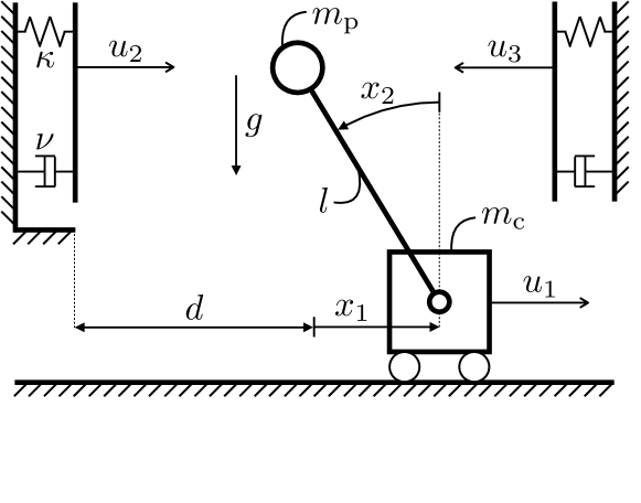
Figure 3: Benchmark problem: regulation of the cart-pole system through a force applied to the cart and exploiting contacts with the soft walls.

IX-A Mixed Logical Dynamical Model

We let $x_{1}$ be the position of the cart, $x_{2}$ the angle of the pole, and we denote with $x_{3}$ and $x_{4}$ their time derivatives. The force applied to the cart is $u_{1}$, whereas the contact forces with the left and right walls are $u_{2}$ and $u_{3}$, respectively. The continuous-time equations of motion, linearized around the nominal angle of the pole $x_{2}=0$, are

$$\dot{x}_{1} =x_{3},$$ (21a)

$$\dot{x}_{2} =x_{4},$$ (21b)

$$\dot{x}_{3} =\frac{m_{\mathrm{p}}g}{m_{\mathrm{c}}}x_{2}+\frac{1}{m_{\mathrm{c}}}u_{1},$$ (21c)

$$\dot{x}_{4} =\frac{(m_{\mathrm{c}}+m_{\mathrm{p}})g}{m_{\mathrm{c}}l}x_{2}+\frac{1}{m_{\mathrm{c}}l}u_{1}-\frac{1}{m_{\mathrm{p}}l}u_{2}+\frac{1}{m_{\mathrm{p}}l}u_{3},$$ (21d)

with $m_{\mathrm{c}}=m_{\mathrm{p}}=1$ mass of the cart and the pole, $g=10$ gravity acceleration, and $l=1$ length of the pole. Dynamics are discretized using the explicit Euler method with time step $h=0.05$. The force applied to the cart and the system state are subject to the constrains $\underaccent{\bar{}}{u}_{1}\leq u_{1}\leq\bar{u}_{1}$ and $\underaccent{\bar{}}{x}\leq x\leq\bar{x}$, where $\bar{u}_{1}=-\underaccent{\bar{}}{u}_{1}=1$, $\bar{x}=-\underaccent{\bar{}}{x}=(d,\pi/10,1,1)$ , and $d=0.5$ is half of the distance between the walls (see Figure 3).

Impacts between the pole and the walls are modeled with soft contacts: $\kappa=100$ is the stiffness and $\nu=10$ is the damping in the contact model. The position of the tip of the pole with respect to the walls (positive in case of penetration), after linearization, is $\delta_{2}:=-x_{1}+lx_{2}-d$ for the left wall, and $\delta_{3}:=x_{1}-lx_{2}-d$ for the right wall. For $i\in\{2,3\}$, contact forces are required to obey the constitutive model

$$u_{i}=\begin{cases}\kappa\delta_{i}+\nu\dot{\delta}_{i}&\text{if}\ \delta_{i}\geq 0\ \text{and}\ \kappa\delta_{i}+\nu\dot{\delta}_{i}\geq 0,\\ 0&\text{otherwise}.\end{cases}$$ (22)

These conditions ensure that contact forces are nonzero only in case of penetration, and are always nonnegative (i.e., the walls never pull on the pole). To model these piecewise-linear functions, we introduce two binary indicators per contact

$$u_{i+2}:=\begin{cases}1&\text{if}\ \delta_{i}\geq 0,\\ 0&\text{otherwise},\end{cases}\quad u_{i+4}:=\begin{cases}1&\text{if}\ \kappa\delta_{i}+\nu\dot{\delta}_{i}\geq 0,\\ 0&\text{otherwise}.\end{cases}$$ (23)

By means of the state limits, we can derive explicit bounds $\underaccent{\bar{}}{\delta}_{i},\bar{\delta}_{i}$ on the penetrations, as well as on their time derivatives $\underaccent{\bar{}}{\dot{\delta}}_{i},\bar{\dot{\delta}}_{i}$. These, in turn, are used to bound the contact forces with $\underaccent{\bar{}}{u}_{i}:=\kappa\underaccent{\bar{}}{\delta}_{i}+\nu\underaccent{\bar{}}{\dot{\delta}}_{i}$ and $\bar{u}_{i}:=\kappa\bar{\delta}_{i}+\nu\bar{\dot{\delta}}_{i}$. Conditions (23) are then enforced through the linear inequalities

$$\underaccent{\bar{}}{\delta}_{i}(1-u_{i+2})\leq\delta_{i}\leq\bar{\delta}_{i}u_{i+2},$$ (24a)

$$\underaccent{\bar{}}{u}_{i}(1-u_{i+4})\leq\kappa\delta_{i}+\nu\dot{\delta}_{i}\leq\bar{u}_{i}u_{i+4}.$$ (24b)

With a similar logic, we can express (22) through the conditions: $u_{i}\geq 0$, $u_{i}\leq\bar{u}_{i}u_{i+2}$, $u_{i}\leq\bar{u}_{i}u_{i+4}$, and

$$\nu\bar{\dot{\delta}}_{i}(u_{i+2}-1)\leq u_{i}-\kappa\delta_{i}-\nu\dot{\delta}_{i}\leq\underaccent{\bar{}}{u}_{i}(u_{i+4}-1).$$ (25)

Considering the binary inputs introduced as contact indicators, we have an MLD system with $n_{x}=4$ states, $n_{u}=3$ continuous inputs, and $m_{u}=4$ binary inputs.

IX-B Model Predictive Controller

We synthesize an MPC controller featuring both a terminal penalty and a terminal constraint (see Section VIII). For the stage cost, we let $Q_{t}=I$ and $R_{t}=(1,0,0,0,0,0,0)^{\prime}$ for $t=0,\ldots,T-1$. Using these weights and setting $u_{2}=u_{3}=0$, the terminal penalty $Q_{T}$ is obtained by solving the Discrete Algebraic Riccati Equation (DARE) for the discretized version of (21). The terminal set is the maximal positive-invariant set for system (21) after discretization, in closed loop with the controller from the DARE and subject to the input and state bounds, and the nonpenetration constraints $\delta_{i}\leq 0$ for $i=2,3$. With a time horizon $T=20$, the resulting MIQP has 224 optimization variables (144 continuous and 80 binaries) and 906 linear constraints (84 equalities and 822 inequalities).

IX-C Branch-and-Bound Implementation

The results we present in this section are obtained with a very basic python implementation of B&B, which follows to the letter the description given in Section III-A. This has the advantage of simplifying result interpretation, since it leaves out of the analysis the many heuristics that come into play when using advanced B&B solvers. Nevertheless, we underline that MILP reoptimization techniques similar in nature to the one we propose have been successfully integrated, e.g., with the state-of-the-art solver SCIP [48] in [39]. The latter work shows how advanced B&B routines (such as presolving, domain propagation, and strong branching) can be handled when reusing the B&B frontier from the previous solves.

In our implementation, we adopt a best-first search: among all the sets which verify condition (5), we pick the set $\mathcal{V}^{i}\in\mathscr{V}^{i}$ for which $\underaccent{\bar{}}{\theta}(\mathcal{V}^{i})$ is minimum. We perform the branching step in chronological order: each time this routine is called, we select the relaxed variables $v_{t\mid\tau}$ for which $t$ is lowest and, among these, we split the one with the smallest index. This frequently-used heuristic, leveraging the control limits, quickly rules out excessively fast mode transitions [34, 23]. Since we include model errors in the upcoming analysis, the recursive-feasibility arguments from Section VI do not apply, and we let $\bar{\theta}^{0}=\infty$ in all the B&B solves. The optimality tolerance $\varepsilon$ in (5) is set to zero. QPs are solved using the dual simplex method provided by the commercial solver Gurobi 9.0.1, with default options. Root-node subproblems are warm started as discussed in Sections V and VIII while, deeper in the B&B tree, subproblems are warm started using the parent active set.

IX-D Statistical Analysis

We test the warm-start algorithm in a “push-recovery” task where, to simulate a push towards the right wall, we set the initial state to $x_{0}:=(0,0,1,0)$. Assuming a perfect model, Figure 4 depicts the optimal control sequence, and the related trajectory of the tip of the pole, for a closed-loop simulation of $50$ steps. The system exploits the (soft) right wall to decelerate and come back to the center of the track, whereas the control requires a significant saturation to accomplish the task.

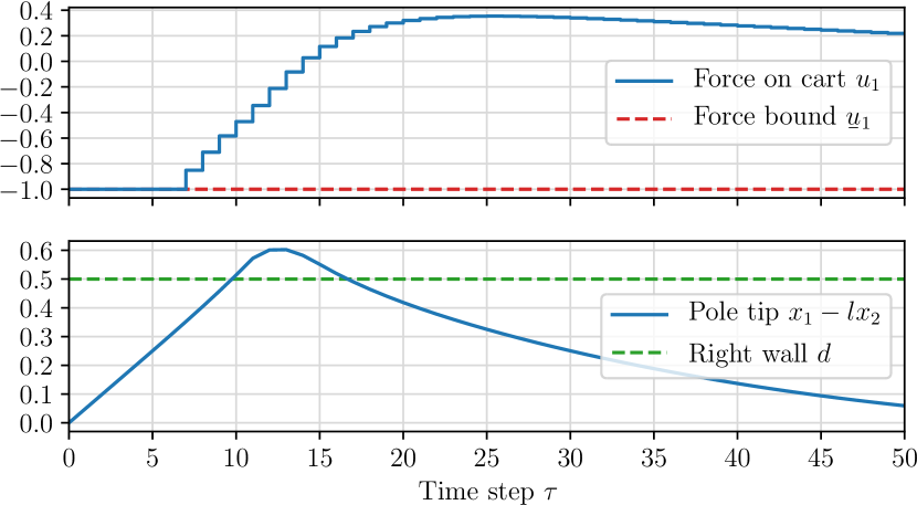
Figure 4: Optimal closed-loop trajectories for the cart-pole system recovering from a push towards the right wall. Top: input force applied to the cart. Bottom: horizontal position of the tip of the pole. The penetration of the pole in the right wall is allowed by the soft contact model.

We study this task in presence of random model errors. At each time $\tau$ we draw the $i$th entry of the error $e_{\tau}:=x_{\tau+1}-Ax_{\tau}-Bu_{\tau}$ from the normal distribution with zero mean and standard deviation $\sigma_{i}=c\bar{x}_{i}$, with $\bar{x}_{i}$ upper bound on the $i$th state. For $c=10^{-3},3\cdot 10^{-3},10^{-2}$, we simulate 100 closed-loop trajectories (for which model errors do not drive the system to an infeasible state) and we monitor the number of QPs solved within B&B and the MIQP solution times.

IX-D1 Number of Branch-and-Bound Subproblems

We start by comparing the number of QPs solved within B&B in case of warm and cold start (i.e., when each MIQP is solved from scratch). Furthermore, to show that the amount of information propagated by the warm starts does not diverge as more and more MIQPs are solved, we analyze the cardinality of the initial covers $\mathscr{V}_{\tau}^{0}$. For these three quantities, Figure 5 reports the minimum, maximum, 80th and 90th percentile of the values registered in the 100 trials. Additionally, Figure 5 shows the results obtained in the nominal case, $e_{\tau}=0$ for all $\tau$.

For small model errors, the warm-start approach almost always requires an order of magnitude less QPs to solve problem (2) to global optimality. Note that, for $c=3\cdot 10^{-3}$, the curve of the 90th percentile almost coincides with the one of the minima. For $c=10^{-2}$ model errors become very significant: we often have mismatches in the cart position greater than $10^{-2}$ which, if multiplied by $\kappa$, lead to variations of the contact forces, with respect to the planned values, greater than the input limit $\bar{u}_{1}=1$. Despite that, $80\%$ of the times the proposed technique reduces the number of QP solves by an order of magnitude. Moreover, even in the worst case, our warm-start algorithm outperforms the cold-start approach.

The asymptotic behavior discussed in Section VII is also found in Figure 5. To solve a problem with $m$ binaries, in fact, the minimum number of B&B subproblems is $2m+1$ (the optimal branch plus the necessary leaves) and, in case of warm start, the best-case complexity of a one-step look-ahead problem ($2m_{u}+1=9$ subproblems) is frequently approached.

The amount of information contained in the warm starts, measured as the cardinality of $\mathscr{V}_{\tau}^{0}$, is very stable both in time $\tau$ and as a function of the error standard deviation $\sigma_{i}$.

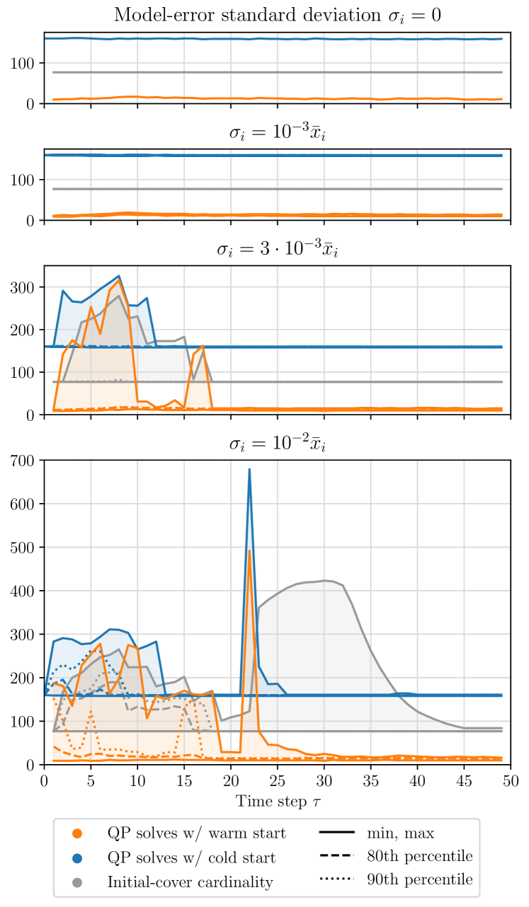
Figure 5: Statistical analysis of the number of B&B subproblems necessary to solve the MIQP (2) and regulate the cart-pole system to the origin. Orange and blue lines: number of QP solves with warm and cold start, respectively, as functions of time and for different standard deviations of the model error $e_{\tau}$. Gray lines: amount of information propagated between time steps by the warm start (represented by the cardinality of the initial cover $\mathscr{V}_{\tau}^{0}$) as a function of time and the error standard deviation. Solid, dashed, and dotted lines: minimum and maximum, 80th percentile, and 90th percentile, respectively, of the above quantities over 100 feasible trial trajectories.

IX-D2 Computation Times

In Figure 6 we illustrate the computation times of the statistical analysis. We compare three alternatives to solve problem (2): the proposed warm-start algorithm, its cold-started counterpart, and the state-of-the-art solver Gurobi 9.0.1. Together with these, we report the time delay in the solution of (2) due to the construction of the warm start.

For our implementation of B&B, both warm and cold started, in Figure 6 we report only the time spent solving QPs (retrieved via the Runtime attribute of the Gurobi QP model). This because almost the totality of the remaining time is spent within the gurobipy interface, doing array manipulations in numpy, or within python list comprehensions. Currently, QP solves take around 15% of the overall B&B function-call time. However, with a more mature implementation (e.g., in C++) we expect to reduce this overhead by two orders of magnitude, making it one order of magnitude smaller than the QP solve times. For the warm-start construction times, we separate computations that can be done in the background of the time step $h$ (such as the assembly of the initial cover), and computations that require the knowledge of the current state $x_{\tau}$. In Figure 6 we report only the second: despite the unoptimized python implementation, in this analysis, the first take just a few milliseconds (median $3$ ms, maximum $24$ ms), which is smaller than the MIQP solve times and, hence, of any reasonable sampling time $h$.

We let Gurobi run with default options and, to maximize its performance, we use the shifted optimal solution from the previous time step as initial guess for the binary variables (this is used by the Gurobi heuristics to attempt to build an initial binary assignment). More precisely, we set the initial guess $v_{t\mid\tau+1}=v_{t+1\mid\tau}^{*}$ for $t=0,\ldots,T-2$ and $v_{T-1\mid\tau+1}=0$ (where $0$ is the equilibrium value of the binary inputs).

The comparison between warm and cold start is in line with the one above: the great majority of the times the warm-started B&B is an order of magnitude faster and, even in the worst case, it is not slower than the cold-started one. When warm started, our implementation frequently approaches the solution times of Gurobi, which is widely recognised to be the baseline solver for hybrid MPC [31, 30, 33, 32, 35]. This is a promising result, especially considering that our implementation is single threaded, whereas we let Gurobi run on 16 threads. Additionally, Gurobi makes a heavy use of presolve techniques and heuristics that our implementation does not feature. Finally, we highlight that the delays in the MIQP solves due to the construction of the warm starts are negligible since they require, in the worst case, $10^{-3}$ s.

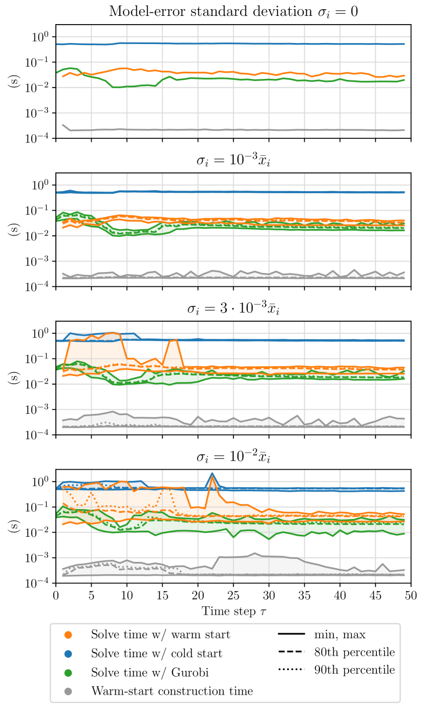
Figure 6: Statistical analysis of the solution times for problem (2). Orange, blue, and green lines: solve times with warm start, cold start, and Gurobi, respectively, as functions of time and for different standard deviations of the model error $e_{\tau}$. (Gurobi runs with default options and is allowed to use the shifted solution from the previous time step as initial guess.) Gray lines: delay in the solution of the MIQPs due to the construction of the warm start as a function of time and the error standard deviation. Solid, dashed, and dotted lines: minimum and maximum, 80th percentile, and 90th percentile, respectively, of the above quantities over 100 feasible trial trajectories.

X Conclusions

The solution of a hybrid MPC problem via B&B generally amounts to a very large number of convex optimizations. In this paper we have shown how, leveraging the receding-horizon structure of the problem, computations performed at one time step can be efficiently reused to warm start subsequent solves, greatly reducing the number of B&B subproblems.

A warm start for a B&B solver should include three elements: a collection of sets which covers the search space, a lower bound on the problem objective in each of these sets, and an upper bound on the problem optimal value. We have shown how the first can be generated by a simple shift in time of the B&B frontier from the previous solve. For the second we have used duality: dual solutions of the B&B frontier, if properly shifted, lead to lower bounds for the leaves of the new problem, even in presence of arbitrary model errors. Finally, we have illustrated how standard persistent-feasibility arguments can be applied to synthesize the third element. All these three ingredients take a negligible time to be computed.

We have thoroughly analyzed the tightness of the bounds we derived, revealing a connection between them and the decrease rate of the MPC cost to go. This has led to the observation that, as the problem horizon grows to infinity, the complexity of the hybrid MPC problem tends to that of a one-step look-ahead problem. In this case, the warm-started B&B needs to reoptimize only the final stage of the control problem.

Theoretical results have been validated by a thorough statistical analysis. The latter has demonstrated that our method greatly outperforms the standard approach of solving each optimization problem from scratch.

Appendix A Extensions and Additional Applications

We collect here extensions and additional applications of the proposed algorithm. In Appendix A-A we extend the results to the case in which the MLD system to be controlled has binary states. Appendix A-B deals with time-varying MLD systems. Finally, in Appendix A-C, we analyze the case in which the prediction horizon $T$ is included among the decision variables of the MPC problem (2).

A-A MLD System with Binary States

As discussed in Section II-A, auxiliary inputs can be used to constrain state components to assume binary values. However, this approach might be suboptimal from the viewpoint of computational efficiency: in this appendix, we show how binary states can be explicitly included in the analysis.

We consider the state vector $x_{\tau}\in\mathbb{R}^{n_{x}}\times\{0,1\}^{m_{x}}$, and we denote by $y_{\tau}\in\{0,1\}^{m_{x}}$ its binary entries. We define the selection matrix $Y$ so that $y_{\tau}=Yx_{\tau}$. The error vector $e_{\tau}$ takes now values in $\mathbb{R}^{n_{x}}\times\{-1,0,1\}^{m_{x}}$. In these settings, problem (2) must include the additional constraint $Yx_{t\mid\tau}\in\{0,1\}^{m_{x}}$ for $t=0,\ldots,T$, and B&B needs to find a cover of $\{0,1\}^{(T+1)m_{x}+Tm_{u}}$. In the convex relaxation of $\mathbf{P}_{\tau}$, we have the additional constraints $\underaccent{\bar{}}{y}_{t\mid\tau}\leq Yx_{t\mid\tau}\leq\bar{y}_{t\mid\tau}$ for $t=0,\ldots,T$, where $\underaccent{\bar{}}{y}_{t\mid\tau},\bar{y}_{t\mid\tau}\in\{0,1\}^{m_{x}}$ and $\underaccent{\bar{}}{y}_{t\mid\tau}\leq\bar{y}_{t\mid\tau}$. Let $\underaccent{\bar{}}{\xi}_{t\mid\tau}$ and $\bar{\xi}_{t\mid\tau}$ be the nonnegative multipliers associated with these constraints. The dual objective (6a) must now include the additional linear term $\sum_{t=0}^{T}(\underaccent{\bar{}}{y}_{t\mid\tau}^{\prime}\underaccent{\bar{}}{\xi}_{t\mid\tau}-\bar{y}_{t\mid\tau}^{\prime}\bar{\xi}_{t\mid\tau})$. Similarly, the terms $Y^{\prime}(\bar{\xi}_{t\mid\tau}-\underaccent{\bar{}}{\xi}_{t\mid\tau})$ and $Y^{\prime}(\bar{\xi}_{T\mid\tau}-\underaccent{\bar{}}{\xi}_{T\mid\tau})$ must be added to the left-hand sides of (6b) and (6c), respectively. The logic behind the shifting procedure from Section IV is the same: the first step requires the additional check $\underaccent{\bar{}}{y}_{0\mid 0}\leq y_{0}\leq\bar{y}_{0\mid 0}$, the second generates the additional bounds $(\underaccent{\bar{}}{y}_{1\mid 0},\ldots,\underaccent{\bar{}}{y}_{T\mid 0},0,\ldots,0)$, $(\bar{y}_{1\mid 0},\ldots,\bar{y}_{T\mid 0},1,\ldots,1)$. In Lemma 1, we define $(\underaccent{\bar{}}{\xi}_{t\mid 1},\bar{\xi}_{t\mid 1}):=(\underaccent{\bar{}}{\xi}_{t+1\mid 0},\bar{\xi}_{t+1\mid 0})$ for $t=0,\ldots,T-1$, and $(\underaccent{\bar{}}{\xi}_{T\mid 1},\bar{\xi}_{T\mid 1}):=0$. In Theorem 1, we add to $\pi_{3}$ the nonnegative term $(y_{0}-\underaccent{\bar{}}{y}_{0\mid 0})^{\prime}\underaccent{\bar{}}{\xi}_{0\mid 0}+(\bar{y}_{0\mid 0}-y_{0})^{\prime}\bar{\xi}_{0\mid 0}$, whereas Corollary 1 remains unchanged. In Section VI, we just need the additional condition $Yx\in\{0,1\}^{m_{x}}$ for control invariance. The asymptotic analysis from Section VII and the extensions in Sections VIII do not require any modification.

A-B Time-Varying MLD System

All the results presented in this paper can be immediately generalized to the case of a time-varying MLD system

$$x_{\tau+1}=A_{\tau}x_{\tau}+B_{\tau}u_{\tau}+e_{\tau},\quad(x_{\tau},u_{\tau})\in\mathcal{D}_{\tau}.$$ (26)

Dynamics of this kind appear, e.g., in trajectory tracking or local stabilization of limit cycles for hybrid nonlinear systems. These are two common problems in robotics, where state-of-the-art methods cannot reason yet about online modifications of the preplanned switching sequence [50, 51, 52, 53].

In this case, the dynamics (2c) becomes $x_{t+1\mid\tau}=A_{\tau+t}x_{t\mid\tau}+B_{\tau+t}u_{t\mid\tau}$, the constraint (2d) reads $(x_{t\mid\tau},u_{t\mid\tau})\in\mathcal{D}_{\tau+t}$, and the weight matrices $Q_{\tau+t}$ and $R_{\tau+t}$ can vary with the absolute time $\tau+t$. Note that this time dependency is easier to handle than the one discussed in Section VIII. There, problem data depend on the relative time $t$ and they can disagree after a shift of the MPC time window (e.g., the matrix $Q_{t+1}$ in problem $\mathbf{P}_{\tau}$ might be different from $Q_{t}$ in $\mathbf{P}_{\tau+1}$). Here, problem data still match after a window shift, and procedures like the one from Lemma 1 do not break.

The dual problem (6) does not change structure, it only requires a suitable modification of the subscripts of the matrices in it. The shifting procedure in Section IV does not need any adjustment. The results from Section V are also still valid, provided that we add the subscript $0$ to the matrices $Q$, $R$, $F$, $G$, and $h$ in the statement of Theorem 1. Also the persistent-feasibility argument from Section VI extends to the time-varying case: we now have a sequence of control-invariant sets $\mathcal{X}_{\tau}$ and, for all $x$ in $\mathcal{X}_{\tau}$, there must exists a $u\in\mathbb{R}^{n_{u}}\times\{0,1\}^{m_{u}}$ such that $(x,u)\in\mathcal{D}_{\tau+T}$ and $A_{\tau+T}x+B_{\tau+T}u\in\mathcal{X}_{\tau+1}$. The asymptotic considerations from Section VII need only a couple of adjustments: $Q$ and $R$ in Lemma 2 must be substituted with $Q_{0}$ and $R_{0}$, and the invariance argument in Theorem 2 must be revised as just shown with persistent feasibility.

The extension of the results from Section VIII is slightly more involved. The weight matrices and the constraint sets depend now on $\tau$ and $t$ independently: we use the notation $Q_{t\mid\tau}$, $R_{t\mid\tau}$, $\mathcal{D}_{t\mid\tau}$ for the data of problem $\mathbf{P}_{\tau}$ at time $t$. Note that, e.g., a terminal penalty implies $Q_{T\mid\tau}\neq Q_{T-1\mid\tau+1}$. Assumption 1 must now require that the row space of $Q_{t\mid\tau+1}$ and $R_{t\mid\tau+1}$ contains the one of $Q_{t+1\mid\tau}$ and $R_{t+1\mid\tau}$, respectively. Then, the generalization presented in Section VIII-A also applies to the time-varying case if, e.g., instead of the matrices $Q_{t}$ and $Q_{t+1}$, we consider $Q_{t\mid 1}$ and $Q_{t+1\mid 0}$. Analogous changes are required for Assumption 2 and the results from Section VIII-B.

A-C Variable-Horizon MPC

In many applications, it is desirable to include the time horizon $T$ among the decision variables of the MPC problem. Besides avoiding the tricky compromise of fixing a value for $T$, this guarantees persistent feasibility and minimizes the discrepancy between open- and closed-loop trajectories [54, 55]. Additionally, it extends the scope of MPC beyond regulation problems [56].

A common problem statement for variable-horizon MPC is to find a control sequence that drives the system state to a target set, despite disturbances and minimizing a weighted sum of the reach time and the control effort [56, 57, Section 2.4]. In [56] this problem has been transcribed in mixed-integer form by parameterizing the reach time with binary variables $b_{t\mid\tau}$ ($b_{t\mid\tau}=1$ when the target set is reached, and $b_{t\mid\tau}=0$ otherwise). Because of coupling constraints between the binaries of different time steps (e.g., $\sum_{t=0}^{T}b_{t\mid\tau}=1$), the formulation in [56] does not have the form of an optimal control problem of MLD systems. However, equivalent binary parameterizations that enjoy this property can be easily found, resulting in a problem of the form we considered in Section VIII and allowing the use of the proposed warm-start technique.

Appendix B Lagrangian Dual of the Convex Relaxation of (2)

In this appendix we derive the dual $\mathbf{D}(\mathcal{V})$ of the convex relaxation $\mathbf{P}(\mathcal{V})$ of problem (2), with $\mathcal{V}$ defined in (4). We describe this derivation since the nonstrict convexity of $\mathbf{P}(\mathcal{V})$ requires some special care.

We start by introducing the auxiliary primal variables

$$z_{t\mid\tau}:=Qx_{t\mid\tau}, t=0,\ldots,T,$$ (27a)

$$w_{t\mid\tau}:=Ru_{t\mid\tau}, t=0,\ldots,T-1.$$ (27b)

After substituting these in the primal objective (2a), we define the Lagrangian function

$$l:= \ \sum_{t=0}^{T}[|z_{t\mid\tau}|^{2}+\rho_{t\mid\tau}^{\prime}(Qx_{t\mid\tau}-z_{t\mid\tau})]$$

$$+\sum_{t=0}^{T-1}[|w_{t\mid\tau}|^{2}+\sigma_{t\mid\tau}^{\prime}(Ru_{t\mid\tau}-w_{t\mid\tau})]+\lambda_{0\mid\tau}^{\prime}(x_{0\mid\tau}-x_{\tau})$$

$$+\sum_{t=0}^{T-1}\lambda_{t+1\mid\tau}^{\prime}(x_{t+1\mid\tau}-Ax_{t\mid\tau}-Bu_{t\mid\tau})$$

$$+\sum_{t=0}^{T-1}\mu_{t\mid\tau}^{\prime}(Fx_{t\mid\tau}+Gu_{t\mid\tau}-h)$$

$$+\sum_{t=0}^{T-1}[\underaccent{\bar{}}{\nu}_{t\mid\tau}^{\prime}(\underaccent{\bar{}}{v}_{t\mid\tau}-Vu_{t\mid\tau})+\bar{\nu}_{t\mid\tau}^{\prime}(Vu_{t\mid\tau}-\bar{v}_{t\mid\tau})],$$ (28)

with $\{\lambda_{t\mid\tau},\rho_{t\mid\tau}\}_{t=0}^{T}$ and $\{\mu_{t\mid\tau},\underaccent{\bar{}}{\nu}_{t\mid\tau},\bar{\nu}_{t\mid\tau},\sigma_{t\mid\tau}\}_{t=0}^{T-1}$ Lagrange multipliers of appropriate dimensions. For any fixed value of the multipliers such that the nonnegativity condition (6e) holds, the infimum of the Lagrangian with respect to the primal variables yields a lower bound on the optimal value $\theta(\mathcal{V})$. We seek the multipliers for which this lower bound is maximum.

For the outer maximization to be feasible (i.e., have an optimal value greater than $-\infty$), we must require the inner minimization to be bounded. Since the Lagrangian is a convex quadratic function of the primal variables, its infimum, if finite, verifies the stationarity conditions $\nabla_{x_{t\mid\tau}}l=0$ (corresponding to (6b) and (6c)), $\nabla_{u_{t\mid\tau}}l=0$ (corresponding to (6d)), and

$$\nabla_{z_{t\mid\tau}}l=2z_{t\mid\tau}-\rho_{t\mid\tau}=0, t=0,\ldots,T,$$ (29a)

$$\nabla_{w_{t\mid\tau}}l=2w_{t\mid\tau}-\sigma_{t\mid\tau}=0, t=0,\ldots,T-1.$$ (29b)

Substituting the stationarity conditions in the Lagrangian (28), we obtain its minimum value (6a). The dual problem $\mathbf{D}(\mathcal{V})$ consists then in the maximization of (6a), subject to the stationarity conditions and the nonnegativity of the multipliers $\{\mu_{t\mid\tau},\underaccent{\bar{}}{\nu}_{t\mid\tau},\bar{\nu}_{t\mid\tau}\}_{t=0}^{T-1}$. Conditions (29) are removed from the dual problem because they are redundant.

Appendix C Proof of Theorem 1

In this appendix we derive the lower bound (12). Given a feasible solution for $\mathbf{D}_{0}(\mathcal{V}_{0})$ we define a set of feasible multipliers for $\mathbf{D}_{1}(\mathcal{V}_{1})$ as in Lemma 1. Substituting these into the objective (6a) of the latter problem, we get the lower bound

$$\underaccent{\bar{}}{\theta}_{1}(\mathcal{V}_{1}):=-\sum_{t=0}^{T-1}|\rho_{t+1\mid 0}/2|^{2}-\sum_{t=0}^{T-2}|\sigma_{t+1\mid 0}/2|^{2}-x_{1}^{\prime}\lambda_{1\mid 0}\\ -\sum_{t=0}^{T-2}(h^{\prime}\mu_{t+1\mid 0}+\bar{v}_{t+1\mid 0}^{\prime}\bar{\nu}_{t+1\mid 0}-\underaccent{\bar{}}{v}_{t+1\mid 0}^{\prime}\underaccent{\bar{}}{\nu}_{t+1\mid 0}).$$ (30)

The cost of the candidate solution can be restated as $\underaccent{\bar{}}{\theta}_{1}(\mathcal{V}_{1})=\underaccent{\bar{}}{\theta}_{0}(\mathcal{V}_{0})+\sum_{i=1}^{3}\omega_{i}$, where

$$\omega_{1}:=\ x_{0}^{\prime}\lambda_{0\mid 0}-x_{1}^{\prime}\lambda_{1\mid 0},$$ (31a)

$$\omega_{2}:=\ h^{\prime}\mu_{0\mid 0}+\bar{v}_{0\mid 0}^{\prime}\bar{\nu}_{0\mid 0}-\underaccent{\bar{}}{v}_{0\mid 0}^{\prime}\underaccent{\bar{}}{\nu}_{0\mid 0},$$ (31b)

$$\omega_{3}:=\ |\rho_{0\mid 0}/2|^{2}+|\sigma_{0\mid 0}/2|^{2}.$$ (31c)

Enforcing the dynamics, we get

$$\omega_{1}=x_{0}^{\prime}\lambda_{0\mid 0}-(Ax_{0}+Bu_{0}+e_{0})^{\prime}\lambda_{1\mid 0},$$ (32)

and using (6b) and (6d) for $t=\tau=0$, we have

$$\omega_{1}=-x_{0}^{\prime}(Q^{\prime}\rho_{0\mid 0}+F^{\prime}\mu_{0\mid 0})\\ -u_{0}^{\prime}[R^{\prime}\sigma_{0\mid 0}+G^{\prime}\mu_{0\mid 0}+V^{\prime}(\bar{\nu}_{0\mid 0}-\underaccent{\bar{}}{\nu}_{0\mid 0})]+\pi_{4}.$$ (33)

Adding $\omega_{2}$, we obtain

$$\omega_{1}+\omega_{2}=-x_{0}^{\prime}Q^{\prime}\rho_{0\mid 0}-u_{0}^{\prime}R^{\prime}\sigma_{0\mid 0}+\pi_{3}+\pi_{4}.$$ (34)

Finally, we add $\omega_{3}$:

$$\sum_{i=1}^{3}\omega_{i}=|\rho_{0\mid 0}/2|^{2}-x_{0}^{\prime}Q^{\prime}\rho_{0\mid 0}+|\sigma_{0\mid 0}/2|^{2}-u_{0}^{\prime}R^{\prime}\sigma_{0\mid 0}\\ +\pi_{3}+\pi_{4}.$$ (35)

Using the identities

$$|\rho_{0\mid 0}/2|^{2}-x_{0}^{\prime}Q^{\prime}\rho_{0\mid 0} =|\rho_{0\mid 0}/2-Qx_{0}|^{2}-|Qx_{0}|^{2},$$ (36a)

$$|\sigma_{0\mid 0}/2|^{2}-u_{0}^{\prime}R^{\prime}\sigma_{0\mid 0} =|\sigma_{0\mid 0}/2-Ru_{0}|^{2}-|R_{0}u_{0}|^{2},$$ (36b)

and recalling the definition of $\pi_{1}$ and $\pi_{2}$, we obtain $\sum_{i=1}^{3}\omega_{i}=\sum_{i=1}^{4}\pi_{i},$ and hence (12).

Tobia Marcucci graduated cum laude in Mechanical Engineering from the University of Pisa in 2015. From 2015 to 2017 he was Ph.D. student at the Research Center “E. Piaggio”, University of Pisa, and the Istituto Italiano di Tecnologia (IIT). Since 2017 he is at the Computer Science and Artificial Intelligence Laboratory (CSAIL), MIT, to continue his Ph.D. studies. His main research interests are robotics, control theory, and numerical optimization.

Russ Tedrake is the Toyota Professor of Electrical Engineering and Computer Science, Aeronautics and Astronautics, and Mechanical Engineering at MIT, the Director of the Center for Robotics at CSAIL, and the leader of Team MIT’s entry in the DARPA Robotics Challenge. Russ is also the Vice President of Robotics Research at the Toyota Research Institute. He is a recipient of the NSF CAREER Award, the MIT Jerome Saltzer Award for undergraduate teaching, the DARPA Young Faculty Award in Mathematics, the 2012 Ruth and Joel Spira Teaching Award, and was named a Microsoft Research New Faculty Fellow. Russ received his B.S.E. in Computer Engineering from the University of Michigan, Ann Arbor, in 1999, and his Ph.D. in Electrical Engineering and Computer Science from MIT in 2004, working with Sebastian Seung. After graduation, he joined the MIT Brain and Cognitive Sciences Department as a Postdoctoral Associate. During his education, he has also spent time at Microsoft, Microsoft Research, and the Santa Fe Institute.

References

- [1] D. Q. Mayne, J. B. Rawlings, C. V. Rao, and P. O. Scokaert, “Constrained model predictive control: Stability and optimality,” Automatica, vol. 36, no. 6, pp. 789–814, 2000.
- [2] A. Bemporad and M. Morari, “Control of systems integrating logic, dynamics, and constraints,” Automatica, vol. 35, no. 3, pp. 407–427, 1999.
- [3] M. Diehl, H. G. Bock, and J. P. Schlöder, “A real-time iteration scheme for nonlinear optimization in optimal feedback control,” SIAM Journal on control and optimization, vol. 43, no. 5, pp. 1714–1736, 2005.
- [4] M. Conforti, G. Cornuéjols, and G. Zambelli, Integer programming. Springer, 2014, vol. 271.
- [5] R. Fletcher and S. Leyffer, “Numerical experience with lower bounds for miqp branch-and-bound,” SIAM Journal on Optimization, vol. 8, no. 2, pp. 604–616, 1998.
- [6] T. Marcucci and R. Tedrake, “Mixed-integer formulations for optimal control of piecewise-affine systems,” in ACM International Conference on Hybrid Systems: Computation and Control, 2019, pp. 230–239.
- [7] C. V. Rao, S. J. Wright, and J. B. Rawlings, “Application of interior-point methods to model predictive control,” Journal of optimization theory and applications, vol. 99, no. 3, pp. 723–757, 1998.
- [8] H. J. Ferreau, H. G. Bock, and M. Diehl, “An online active set strategy to overcome the limitations of explicit mpc,” International Journal of Robust and Nonlinear Control, vol. 18, no. 8, pp. 816–830, 2008.
- [9] S. Kuindersma, F. Permenter, and R. Tedrake, “An efficiently solvable quadratic program for stabilizing dynamic locomotion,” in International Conference on Robotics and Automation. IEEE, 2014, pp. 2589–2594.
- [10] B. Stellato, G. Banjac, P. Goulart, A. Bemporad, and S. Boyd, “Osqp: An operator splitting solver for quadratic programs,” Mathematical Programming Computation, pp. 1–36, 2020.
- [11] D. Liao-McPherson and I. Kolmanovsky, “Fbstab: A proximally stabilized semismooth algorithm for convex quadratic programming,” Automatica, vol. 113, no. 108801, 2020.
- [12] V. Dua, N. A. Bozinis, and E. N. Pistikopoulos, “A multiparametric programming approach for mixed-integer quadratic engineering problems,” Computers & Chemical Engineering, vol. 26, no. 4-5, pp. 715–733, 2002.
- [13] F. Borrelli, M. Baotić, A. Bemporad, and M. Morari, “Dynamic programming for constrained optimal control of discrete-time linear hybrid systems,” Automatica, vol. 41, no. 10, pp. 1709–1721, 2005.
- [14] R. Oberdieck and E. N. Pistikopoulos, “Explicit hybrid model-predictive control: The exact solution,” Automatica, vol. 58, pp. 152–159, 2015.
- [15] T. Gueddar and V. Dua, “Approximate multi-parametric programming based b&b algorithm for minlps,” Computers & chemical engineering, vol. 42, pp. 288–297, 2012.
- [16] V. M. Charitopoulos and V. Dua, “Explicit model predictive control of hybrid systems and multiparametric mixed integer polynomial programming,” AIChE Journal, vol. 62, no. 9, pp. 3441–3460, 2016.
- [17] D. Axehill, T. Besselmann, D. M. Raimondo, and M. Morari, “A parametric branch and bound approach to suboptimal explicit hybrid mpc,” Automatica, vol. 50, no. 1, pp. 240–246, 2014.
- [18] T. Marcucci, R. Deits, M. Gabiccini, A. Bicchi, and R. Tedrake, “Approximate hybrid model predictive control for multi-contact push recovery in complex environments,” in International Conference on Humanoid Robotics. IEEE, 2017, pp. 31–38.
- [19] S. Sadraddini and R. Tedrake, “Sampling-based polytopic trees for approximate optimal control of piecewise affine systems,” in International Conference on Robotics and Automation. IEEE, 2019, pp. 7690–7696.
- [20] S. Sager, H. G. Bock, and G. Reinelt, “Direct methods with maximal lower bound for mixed-integer optimal control problems,” Mathematical Programming, vol. 118, no. 1, pp. 109–149, 2009.
- [21] S. Sager, M. Jung, and C. Kirches, “Combinatorial integral approximation,” Mathematical Methods of Operations Research, vol. 73, no. 3, p. 363, 2011.
- [22] M. N. Jung, G. Reinelt, and S. Sager, “The lagrangian relaxation for the combinatorial integral approximation problem,” Optimization Methods and Software, vol. 30, no. 1, pp. 54–80, 2015.
- [23] D. Frick, A. Domahidi, and M. Morari, “Embedded optimization for mixed logical dynamical systems,” Computers & Chemical Engineering, vol. 72, pp. 21–33, 2015.
- [24] A. Bürger, C. Zeile, A. Altmann-Dieses, S. Sager, and M. Diehl, “Design, implementation and simulation of an mpc algorithm for switched nonlinear systems under combinatorial constraints,” Journal of Process Control, vol. 81, pp. 15–30, 2019.
- [25] R. Takapoui, N. Moehle, S. Boyd, and A. Bemporad, “A simple effective heuristic for embedded mixed-integer quadratic programming,” International Journal of Control, pp. 1–11, 2017.
- [26] D. Frick, A. Georghiou, J. L. Jerez, A. Domahidi, and M. Morari, “Low-complexity method for hybrid mpc with local guarantees,” SIAM Journal on Control and Optimization, vol. 57, no. 4, pp. 2328–2361, 2019.
- [27] F. Borrelli, A. Bemporad, and M. Morari, Predictive control for linear and hybrid systems. Cambridge University Press, 2017.
- [28] D. Axehill and A. Hansson, “A mixed integer dual quadratic programming algorithm tailored for mpc,” in Conference on Decision and Control. IEEE, 2006, pp. 5693–5698.
- [29] ——, “A dual gradient projection quadratic programming algorithm tailored for model predictive control,” in Conference on Decision and Control. IEEE, 2008, pp. 3057–3064.
- [30] V. V. Naik and A. Bemporad, “Embedded mixed-integer quadratic optimization using accelerated dual gradient projection,” IFAC-PapersOnLine, vol. 50, no. 1, pp. 10 723–10 728, 2017.
- [31] A. Bemporad, “Solving mixed-integer quadratic programs via nonnegative least squares,” IFAC-PapersOnLine, vol. 48, no. 23, pp. 73–79, 2015.
- [32] A. Bemporad and V. V. Naik, “A numerically robust mixed-integer quadratic programming solver for embedded hybrid model predictive control,” IFAC-PapersOnLine, vol. 51, no. 20, pp. 412–417, 2018.
- [33] B. Stellato, V. V. Naik, A. Bemporad, P. Goulart, and S. Boyd, “Embedded mixed-integer quadratic optimization using the osqp solver,” in European Control Conference. IEEE, 2018, pp. 1536–1541.
- [34] A. Bemporad, D. Mignone, and M. Morari, “An efficient branch and bound algorithm for state estimation and control of hybrid systems,” in European Control Conference. IEEE, 1999, pp. 557–562.
- [35] P. Hespanhol, R. Quirynen, and S. Di Cairano, “A structure exploiting branch-and-bound algorithm for mixed-integer model predictive control,” in European Control Conference. IEEE, 2019, pp. 2763–2768.
- [36] A. Del Pia, S. S. Dey, and M. Molinaro, “Mixed-integer quadratic programming is in np,” Mathematical Programming, vol. 162, no. 1-2, pp. 225–240, 2017.
- [37] G. Ausiello, V. Bonifaci, and B. Escoffier, “Complexity and approximation in reoptimization,” in Computability in Context: Computation and Logic in the Real World. World Scientific, 2011, pp. 101–129.
- [38] B. Hiller, T. Klug, and J. Witzig, “Reoptimization in branch-and-bound algorithms with an application to elevator control,” in International Symposium on Experimental Algorithms. Springer, 2013, pp. 378–389.
- [39] G. Gamrath, B. Hiller, and J. Witzig, “Reoptimization techniques for mip solvers,” in International Symposium on Experimental Algorithms. Springer, 2015, pp. 181–192.
- [40] T. Ralphs and M. Güzelsoy, “Duality and warm starting in integer programming,” in NSF Design, Service, and Manufacturing Grantees and Research Conference. Citeseer, 2006.
- [41] A. Bemporad, M. Morari, V. Dua, and E. N. Pistikopoulos, “The explicit linear quadratic regulator for constrained systems,” Automatica, vol. 38, no. 1, pp. 3–20, 2002.
- [42] W. P. Heemels, B. De Schutter, and A. Bemporad, “Equivalence of hybrid dynamical models,” Automatica, vol. 37, no. 7, pp. 1085–1091, 2001.
- [43] C. Buchheim, M. D. Santis, S. Lucidi, F. Rinaldi, and L. Trieu, “A feasible active set method with reoptimization for convex quadratic mixed-integer programming,” SIAM Journal on Optimization, vol. 26, no. 3, pp. 1695–1714, 2016.
- [44] M. Lazar, “Model predictive control of hybrid systems: stability and robustness,” Ph.D. dissertation, Technische Universiteit Eindhoven, 2006.
- [45] E. C. Kerrigan and D. Q. Mayne, “Optimal control of constrained, piecewise affine systems with bounded disturbances,” in Conference on Decision and Control, vol. 2. IEEE, 2002, pp. 1552–1557.
- [46] R. Deits, T. Koolen, and R. Tedrake, “Lvis: Learning from value function intervals for contact-aware robot controllers,” in International Conference on Robotics and Automation. IEEE, 2019, pp. 7762–7768.
- [47] E. G. Gilbert and K. T. Tan, “Linear systems with state and control constraints: The theory and application of maximal output admissible sets,” IEEE Transactions on Automatic control, vol. 36, no. 9, pp. 1008–1020, 1991.
- [48] T. Achterberg, “Scip: solving constraint integer programs,” Mathematical Programming Computation, vol. 1, no. 1, pp. 1–41, 2009.
- [49] G. Frison and J. B. Jørgensen, “Efficient implementation of the riccati recursion for solving linear-quadratic control problems,” in International Conference on Control Applications. IEEE, 2013, pp. 1117–1122.
- [50] R. G. Sanfelice, A. R. Teel, and R. Sepulchre, “A hybrid systems approach to trajectory tracking control for juggling systems,” in Conference on Decision and Control. IEEE, 2007, pp. 5282–5287.
- [51] I. R. Manchester, U. Mettin, F. Iida, and R. Tedrake, “Stable dynamic walking over uneven terrain,” The International Journal of Robotics Research, vol. 30, no. 3, pp. 265–279, 2011.
- [52] I. R. Manchester, “Transverse dynamics and regions of stability for nonlinear hybrid limit cycles,” IFAC Proceedings Volumes, vol. 44, no. 1, pp. 6285–6290, 2011.
- [53] F. Farshidian, M. Kamgarpour, D. Pardo, and J. Buchli, “Sequential linear quadratic optimal control for nonlinear switched systems,” IFAC-PapersOnLine, vol. 50, no. 1, pp. 1463–1469, 2017.
- [54] H. Michalska and D. Q. Mayne, “Robust receding horizon control of constrained nonlinear systems,” IEEE Transactions on Automatic control, vol. 38, no. 11, pp. 1623–1633, 1993.
- [55] P. O. Scokaert and D. Q. Mayne, “Min-max feedback model predictive control for constrained linear systems,” IEEE Transactions on Automatic control, vol. 43, no. 8, pp. 1136–1142, 1998.
- [56] A. Richards and J. P. How, “Robust variable horizon model predictive control for vehicle maneuvering,” International Journal of Robust and Nonlinear Control, vol. 16, no. 7, pp. 333–351, 2006.
- [57] R. C. Shekhar, “Variable horizon model predictive control: robustness and optimality,” Ph.D. dissertation, University of Cambridge, 2012.