Abstract

Quantizing large Neural Networks (nn) while maintaining the performance is highly desirable for resource-limited devices due to reduced memory and time complexity. It is usually formulated as a constrained optimization problem and optimized via a modified version of gradient descent. In this work, by interpreting the continuous parameters (unconstrained) as the dual of the quantized ones, we introduce a Mirror Descent (md)framework (Bubeck, (2015)) for nn quantization. Specifically, we provide conditions on the projections (i.e., mapping from continuous to quantized ones) which would enable us to derive valid mirror maps and in turn the respective md updates. Furthermore, we present a numerically stable implementation of md that requires storing an additional set of auxiliary variables (unconstrained), and show that it is strikingly analogous to the Straight Through Estimator (ste)based method which is typically viewed as a “trick” to avoid vanishing gradients issue. Our experiments on CIFAR-10/100, TinyImageNet, and ImageNet classification datasets with VGG-16, ResNet-18, and MobileNetV2 architectures show that our md variants yield state-of-the-art performance.

1 Introduction

Despite the success of deep neural networks in various domains, their excessive computational and memory requirements limit their practical usability for real-time applications or in resource-limited devices. Quantization is a prominent technique for network compression, where the objective is to learn a network while restricting the parameters (and activations) to take values from a small discrete set. This leads to a dramatic reduction in memory (a factor of $32$ for binary quantization) and inference time – as it enables specialized implementation using bit operations.

Neural Network (nn) quantization is usually formulated as a constrained optimization problem ${\min_{\mathbf{x}\in\mathcal{X}}f(\mathbf{x})},$ where $f(\cdot)$ denotes the loss function by abstracting out the dependency on the dataset and $\mathcal{X}\subset\rm I\!R^{r}$ denotes the set of all possible quantized solutions. Majority of the works in the literature (Ajanthan et al., (2019); Hubara et al., (2017); Yin et al., (2018)) convert this into an unconstrained problem by introducing auxiliary variables ($\tilde{\mathbf{x}}$) and optimize via (stochastic) gradient descent. Specifically, the objective and the update step take the following form:

$$\min_{\tilde{\mathbf{x}}\in\rm I\!R^{r}}f(P(\tilde{\mathbf{x}}))\ ,\quad\tilde{\mathbf{x}}^{k+1}=\tilde{\mathbf{x}}^{k}-\eta\left.\nabla_{\tilde{\mathbf{x}}}f(P(\tilde{\mathbf{x}}))\right|_{\tilde{\mathbf{x}}=\tilde{\mathbf{x}}^{k}}\ ,\\$$ (1)

where $P:\rm I\!R^{r}\to\mathcal{X}$ is a mapping from the unconstrained space to the quantized space (sometimes called projection) and $\eta>0$ is the learning rate. In cases where the mapping $P$ is not differentiable, a suitable approximation is employed (Hubara et al., (2017)).

In this work, by noting that the well-known Mirror Descent (md) algorithm, widely used for online convex optimization (Bubeck, (2015)), provides a theoretical framework to perform gradient descent in the unconstrained space (dual space, $\rm I\!R^{r}$) with gradients computed in the quantized space (primal space, $\mathcal{X}$), we introduce an md framework for nn quantization. In essence, md extends gradient descent to non-Euclidean spaces where Euclidean projection is replaced with a more general projection defined based on the associated distance metric. Briefly, the key ingredient of md is a concept called mirror map which defines both the mapping between primal and dual spaces and the exact form of the projection. Specifically, in this work, by observing $P$ in Eq. (1) as a mapping from dual space to the primal space, we analytically derive corresponding mirror maps under certain conditions on $P$. This enables us to derive different variants of the md algorithm useful for nn quantization.

Note that, md requires the constrained set to be convex, however, the quantization set is discrete. Therefore, as discussed later in Sec. 3, to ensure quantized solutions, we employ a monotonically increasing annealing hyperparameter similar to Ajanthan et al., (2019); Bai et al., (2019). This translates into time-varying mirror maps, and for completeness, we theoretically analyze the convergence behaviour of md in this case for the convex setting. Furthermore, as md is often found to be numerically unstable (Hsieh et al., (2018)), we discuss a numerically stable implementation of md by storing an additional set of auxiliary variables. This update is strikingly analogous to the popular Straight Through Estimator (ste) based gradient method (Bai et al., (2019); Hubara et al., (2017)) which is typically viewed as a “trick” to avoid vanishing gradients issue but here we show that it is an implementation method for md under certain conditions on the mapping $P$. We believe this connection sheds some light on the practical effectiveness of ste.

In summary, we make the following contributions:

• We introduce an md framework with time-varying mirror maps for nn quantization by deriving mirror maps from projections ($P$ in Eq. (1)) and present two md algorithms for quantization.

• Theoretically, we first show that md with time-varying mirror maps converges at the same rate as the standard md in the convex setting. Second, we discuss conditions for the convergence to a discrete solution when a monotonically increasing annealing hyperparameter is employed.

• For practical usability, we introduce a numerically stable implementation of md and show its connection to the popular ste approximation.

• With extensive experiments on CIFAR-10/100, TinyImageNet, and ImageNet classification datasets using VGG-16, ResNet-18, and MobileNetV2 architectures we demonstrate that our md variants yield state-of-the-art performance.

2 Preliminaries

Here we provide a brief background on the md algorithm and nn quantization.

2.1 Mirror Descent

The Mirror Descent (md)algorithm was first introduced in Nemirovsky and Yudin, (1983) and has extensively been studied in the convex optimization literature ever since. In this section, we provide a brief overview and refer the interested reader to Chapter 4 of Bubeck, (2015). In the context of md, we consider a problem of the form:

$$\min_{\mathbf{x}\in\mathcal{X}}\ f(\mathbf{x})\ ,$$ (2)

where $f:\mathcal{X}\to\rm I\!R$ is a convex function and ${\mathcal{X}\subset\rm I\!R^{r}}$ is a compact convex set. The main concept of md is to extend gradient descent to a more general non-Euclidean space (Banach space), thus overcoming the dependency of gradient descent on the Euclidean geometry. The motivation for this generalization is that one might be able to exploit the geometry of the space to optimize much more efficiently. One such example is the simplex constrained optimization where md converges at a much faster rate than the standard Projected Gradient Descent (pgd).

To this end, since the gradients lie in the dual space, optimization is performed by first mapping the primal point $\mathbf{x}^{k}\in\mathcal{B}$ (quantized space, $\mathcal{X}$) to the dual space $\mathcal{B}^{*}$ (unconstrained space, $\rm I\!R^{r}$), then performing gradient descent in the dual space, and finally mapping back the resulting point to the primal space $\mathcal{B}$. If the new point $\mathbf{x}^{k+1}$ lie outside of the constraint set $\mathcal{X}\subset\mathcal{B}$, it is projected to the set $\mathcal{X}$. Both the primal/dual mapping and the projection are determined by the mirror map. Specifically, the gradient of the mirror map defines the mapping from primal to dual and the projection is done via the Bregman divergence of the mirror map. We first provide the definitions for mirror map and Bregman divergence and then turn to the md updates.

Definition 1 (Mirror map).

Let $\mathcal{C}\subset\rm I\!R^{r}$ be a convex open set such that $\mathcal{X}\subset\bar{\mathcal{C}}$ ($\bar{\mathcal{C}}$ denotes the closure of set $\mathcal{C}$) and $\mathcal{X}\cap\mathcal{C}\neq\emptyset$. Then, $\Phi:\mathcal{C}\to\rm I\!R$ is a mirror map if it satisfies:

1. $\Phi$ is strictly convex and differentiable.

2. $\nabla\Phi(\mathcal{C})=\rm I\!R^{r}$, i.e., $\nabla\Phi$ takes all possible values in $\rm I\!R^{r}$.

3. $\lim_{\mathbf{x}\to\partial\mathcal{C}}\|\nabla\Phi(\mathbf{x})\|=\infty$ ($\partial\mathcal{C}$ denotes the boundary of $\mathcal{C}$), i.e., $\nabla\Phi$ diverges on the boundary of $\mathcal{C}$.

Definition 2 (Bregman divergence).

Let $\Phi:\mathcal{C}\to\rm I\!R$ be a continuously differentiable, strictly convex function defined on a convex set $\mathcal{C}$. The Bregman divergence associated with $\Phi$ for points $\mathbf{p},\mathbf{q}\in\mathcal{C}$ is the difference between the value of $\Phi$ at point $\mathbf{p}$ and the value of the first-order Taylor expansion of $\Phi$ around point $\mathbf{q}$ evaluated at point $\mathbf{p}$, i.e.,

$$D_{\Phi}(\mathbf{p},\mathbf{q})=\Phi(\mathbf{p})-\Phi(\mathbf{q})-\left\langle\nabla\Phi(\mathbf{q}),\mathbf{p}-\mathbf{q}\right\rangle\ .\\$$ (3)

Notice, $D_{\Phi}(\mathbf{p},\mathbf{q})\geq 0$ with $D_{\Phi}(\mathbf{p},\mathbf{p})=0$, and $D_{\Phi}(\mathbf{p},\mathbf{q})$ is convex on $\mathbf{p}$.

Now we are ready to provide the mirror descent strategy based on the mirror map $\Phi$. Let ${\mathbf{x}^{0}\in\operatorname*{argmin}_{\mathbf{x}\in\mathcal{X}\cap\mathcal{C}}}\,\Phi(\mathbf{x})$ be the initial point. Then, for iteration $k\geq 0$ and step size $\eta>0$, the update of the md algorithm can be written as:

$$\nabla\Phi(\mathbf{y}^{k+1}) =\nabla\Phi(\mathbf{x}^{k})-\eta\,\mathbf{g}^{k}\ ,$$ (4)

$$\mathbf{x}^{k+1} ={\underset{\mathbf{x}\in\mathcal{X}\cap\mathcal{C}}{\operatorname{argmin}}}\,D_{\Phi}(\mathbf{x},\mathbf{y}^{k+1})\ ,$$

where $\mathbf{g}^{k}\in\partial f(\mathbf{x}^{k})$ and $\mathbf{y}^{k+1}\in\mathcal{C}$. Note that, in Eq. (4), the gradient $\mathbf{g}^{k}$ is computed at $\mathbf{x}^{k}\in\mathcal{X}\cap\mathcal{C}$ (solution space) but the gradient descent is performed in $\rm I\!R^{r}$ (unconstrained dual space). Moreover, by simple algebraic manipulation, it is easy to show that the above md update (4) can be compactly written in a proximal form where the Bregman divergence of the mirror map becomes the proximal term (Beck and Teboulle, (2003)):

$$\mathbf{x}^{k+1} ={\underset{\mathbf{x}\in\mathcal{X}\cap\mathcal{C}}{\operatorname{argmin}}}\,\langle\eta\,\mathbf{g}^{k},\mathbf{x}\rangle+D_{\Phi}(\mathbf{x},\mathbf{x}^{k})\ .$$ (5)

Note, if $\Phi(\mathbf{x})=\frac{1}{2}\left\lVert\mathbf{x}\right\rVert_{2}^{2}$, then $D_{\Phi}(\mathbf{x},\mathbf{x}^{k})=\frac{1}{2}\left\lVert\mathbf{x}-\mathbf{x}^{k}\right\rVert_{2}^{2}$, which when plugged back to the above problem and optimized for $\mathbf{x}$, leads to exactly the same update rule as that of pgd. However, md allows us to choose various forms of $\Phi$ depending on the problem at hand.

2.2 Neural Network Quantization

Neural Network (nn)quantization amounts to training networks with parameters (and activations) restricted to a small discrete set representing the quantization levels. Here we discuss how one can formulate parameter quantization as a constrained optimization problem and activation quantization can be similarly formulated.

Parameter Space Formulation.

Given a dataset $\mathcal{D}=\{\mathbf{x}_{i},\mathbf{y}_{i}\}_{i=1}^{n}$, parameter quantization can be written as:

$$\min_{\mathbf{w}\in\mathcal{Q}^{m}}L(\mathbf{w};\mathcal{D}):=\frac{1}{n}\sum_{i=1}^{n}\ell(\mathbf{w};(\mathbf{x}_{i},\mathbf{y}_{i}))\ .\vspace{-1ex}$$ (6)

Here, $\ell(\cdot)$ denotes the input-output mapping composed with a standard loss function (e.g., cross-entropy loss), $\mathbf{w}$ is the $m$ dimensional parameter vector, and $\mathcal{Q}$ with $|\mathcal{Q}|=d$ is a predefined discrete set representing quantization levels (e.g., $\mathcal{Q}=\{-1,1\}$ or $\mathcal{Q}=\{-1,0,1\}$).

The approaches that directly optimize in the parameter space include BinaryConnect (bc) (Courbariaux et al., (2015)) and its variants (Hubara et al., (2017); Rastegari et al., (2016)), where the constraint set is discrete. In contrast, recent approaches (Bai et al., (2019); Yin et al., (2018)) relax this constraint set to be its convex hull:

$$\operatorname{conv}(\mathcal{Q}^{m})=[q_{\min},q_{\max}]^{m}\ ,$$ (7)

where $q_{\min}$ and $q_{\max}$ represent the minimum and maximum quantization levels, respectively. In this case, a quantized solution is obtained by gradually increasing an annealing hyperparameter.

Lifted Probability Space Formulation.

Another formulation is to treat nn quantization as a discrete labelling problem based on the Markov Random Field (mrf) perspective (Ajanthan et al., (2019)). Here, the equivalent relaxed optimization problem corresponding to Eq. (6) can be written as:

$$\min_{\mathbf{u}\in\Delta^{m}}L(\mathbf{u}\mathbf{q};\mathcal{D}):=\frac{1}{n}\sum_{i=1}^{n}\ell(\mathbf{u}\mathbf{q};(\mathbf{x}_{i},\mathbf{y}_{i}))\ ,$$ (8)

where $\mathbf{q}$ is the vector of quantization levels with $\mathbf{w}=\mathbf{u}\mathbf{q}$ and the set $\Delta^{m}$ takes the following form:

$$\Delta^{m}=\left\{\begin{array}[]{l|l}\hbox{\multirowsetup$\mathbf{u}$}&\sum_{\lambda}u_{j:\lambda}=1,\quad\forall\,j\\ &u_{j:\lambda}\geq 0,\ \ \ \quad\quad\forall\,j,\lambda\end{array}\right\}\ .$$ (9)

We can interpret the value $u_{j:\lambda}$ as the probability of assigning the discrete label $\lambda$ to the weight $w_{j}$. Therefore Eq. (8) can be interpreted as optimizing the probability of each parameter taking a discrete label.

3 Mirror Descent Framework for Network Quantization

Before introducing the md formulation, we first write nn quantization as a single objective unifying (6) and (8) as:

$$\min_{\mathbf{x}\in\mathcal{X}}\ f(\mathbf{x})\ ,$$ (10)

where $f(\cdot)$ denotes the loss function by abstracting out the dependency on the dataset $\mathcal{D}$, and $\mathcal{X}$ denotes the constraint set. As discussed in Sec. 2.2, many recent nn quantization methods optimize over the convex hull of the constraint set. Following this, we consider the solution space $\mathcal{X}$ in Eq. (10) to be convex and compact.

Projection ($P_{\beta_{k}}$)	Space	Mirror Map ($\Phi_{\beta_{k}}$)	Update Step
$\tanh(\beta_{k}\tilde{w})$	$\mathbf{w}$	$\begin{array}[]{ll}\Phi_{\beta_{k}}(w)&=\frac{1}{2\beta_{k}}\big{[}(1+w)\log(1+w)\\ &\qquad+(1-w)\log(1-w)\big{]}\end{array}$	$w^{k+1}=\frac{\frac{1+w^{k}}{1-w^{k}}\exp(-2\beta_{k}\eta g^{k})-1}{\frac{1+w^{k}}{1-w^{k}}\exp(-2\beta_{k}\eta g^{k})+1}$
$\operatorname{softmax}(\beta_{k}\tilde{\mathbf{u}})$	$\mathbf{u}$	$\Phi_{\beta_{k}}(\mathbf{u})=\frac{1}{\beta_{k}}\left[\sum_{\lambda\in\mathcal{Q}}u_{\lambda}\log(u_{\lambda})-u_{\lambda}\right]$	$u^{k+1}_{\lambda}=\frac{u_{\lambda}^{k}\,\exp(-\beta_{k}\eta g^{k}_{\lambda})}{\sum_{\mu\in\mathcal{Q}}\;u_{\mu}^{k}\,\exp(-\beta_{k}\eta g^{k}_{\mu})}\quad\forall\,\lambda\in\mathcal{Q}$

Table 1: Example projections, corresponding mirror maps, and update steps obtained using Theorem 1. Here, $k$ is the iteration index, $\eta>0$ is the learning rate, $g^{k}$ is the gradient of $f$ computed in the primal space, $\beta_{k}\geq 1$ is the annealing hyperparameter, and we assume $m=1$ without loss of generality. Notice the obtained mirror maps vary at each iteration due to $\beta_{k}$ and the $\operatorname{softmax}$ update resembles the popular eda (Beck and Teboulle, (2003)).

To employ md, we need to choose a mirror map (refer Definition 1) suitable for the problem at hand. In fact, as discussed in Sec. 2.1, mirror map is the core component of an md algorithm which determines the effectiveness of the resulting md updates. However, there is no straightforward approach to obtain a mirror map for a given constrained optimization problem, except in certain special cases.

To this end, we observe that the usual approach to optimize the above constrained problem is via a version of projected gradient descent, where the projection is the mapping from the unconstrained auxiliary variables (full-precision) to the quantized space $\mathcal{X}$. Now, noting the analogy between the purpose of the projection operator and the mirror maps in the md formulation, we intend to derive the mirror map analogous to a given projection. Precisely, we prove that if the projection is strictly monotone (and hence invertible), a valid mirror map can be derived from the projection itself. Even though this does not necessarily extend the theory of md, this derivation is valuable as it connects existing pgd type algorithms to their corresponding md variants. For completeness, we state it as a theorem for the case $\mathcal{X}\subset\rm I\!R$ and the multidimensional case can be proved with an additional assumption that the vector field $P^{-1}(\mathbf{x})$ is conservative.

Theorem 1.

Let $\mathcal{C}$ be a finite open interval and ${P:\rm I\!R\to\mathcal{C}}$ be a strictly monotonically increasing continuous function. Then, ${\Phi(x)=\int_{x_{0}}^{x}P^{-1}(y)dy}$ is a valid mirror map.

Proof.

This can be proved by noting that $P$ is invertible, $\nabla\Phi(x)=P^{-1}(x)$, and $\Phi(x)$ is strictly convex. ∎

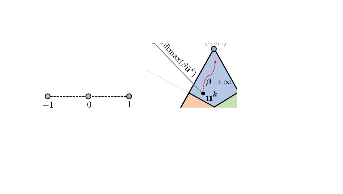
Figure 1: md formulation where mirror map is derived from the projection $P$. Note, $\mathbf{g}^{k}$ is computed in the primal space ($\mathcal{X}$) but it is directly used to update the auxiliary variables in the dual space.

The md update based on the mirror map derived from a given projection is illustrated in Fig. 1. Note that, to employ md to the problem (10), in theory, any mirror map satisfying Definition 1 whose domain (i.e., its closure) is a superset of the constraint set $\mathcal{X}$ can be chosen. The above theorem provides a method to derive a subset of all applicable mirror maps, where the closure of the domain of mirror maps is exactly equal to the constraint set $\mathcal{X}$.

We now provide mirror maps and update steps for two different projections ($\tanh$ for $\mathbf{w}$-space (Eq. (6)) and $\operatorname{softmax}$ for $\mathbf{u}$-space (Eq. (8))) useful for nn quantization in Table 1. Given mirror maps (from Theorem 1), the md updates are straightforwardly derived based on Eq. (5) using kkt conditions (Boyd and Vandenberghe, (2009)). For the detailed derivations and pseudocode for md-$\tanh$, please refer to Appendix. Furthermore, the $\tanh$ projection, its inverse, and the corresponding mirror map are illustrated in Fig. 2, showing monotonicity of the inverse and strict convexity of the derived mirror map.

According to the update steps in Table 1, our md variants corresponding to $\tanh$ and $\operatorname{softmax}$ projections can be performed directly in the primal space. However, for some projections (e.g., multi-bit quantization), it might be non-trivial to derive the exact form of mirror maps (and the md update), nevertheless, the md update can be easily implemented by storing an additional set of auxiliary variables. This as discussed in Sec. 3.2 also improves the numerical stability of md.

Note that, to ensure a discrete solution at the end of the training, the projection $P$ is parametrized by a scalar $\beta_{k}\geq 1$ and it is annealed throughout the optimization. This annealing hyperparameter translates into a time varying mirror map (refer to Table 1) in our case. Intuitively, such an adaptive mirror map gradually constrains the solution space $\mathcal{X}$ to its boundary and in the limit enforces a quantized solution.

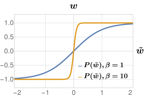
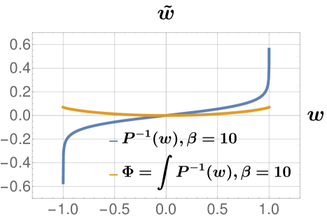
Figure 2: Plots of $\tanh$, its inverse and corresponding mirror map. Note that, the inverse is monotonically increasing and the mirror map is strictly convex. Moreover, when $\beta\to\infty$, $\tanh$ approaches the step function.

3.1 Annealing and Convergence Analysis

The classical md literature studied the convergence behaviour of md for the convex setting, and the adaptive mirror maps are considered in online learning (McMahan, (2017)). We now prove that, in the convex setting, if the annealing hyperparameter $\beta_{k}$ is bounded, then md with an adaptive mirror map converges to the optimal value at the same rate of $\mathcal{O}(1/\sqrt{t})$ as the standard md.

Theorem 2.

Let $\mathcal{X}\subset\rm I\!R^{r}$ be a convex compact set and $\mathcal{C}\subset\rm I\!R^{r}$ be a convex open set with $\mathcal{X}\cap\mathcal{C}\neq\emptyset$ and $\mathcal{X}\subset\bar{\mathcal{C}}$ ( $\bar{\mathcal{C}}$ denotes the closure of $\mathcal{C}$). Let $\Phi:\mathcal{C}\to\rm I\!R$ be a mirror map $\rho$-strongly convex on $\mathcal{X}\cap\mathcal{C}$ with respect to $\left\lVert\cdot\right\rVert$, ${R^{2}=\sup_{\mathbf{x}\in\mathcal{X}\cap\mathcal{C}}\Phi(\mathbf{x})-\Phi(\mathbf{x}^{0})}$ where $\mathbf{x}^{0}=\operatorname*{argmin}_{\mathbf{x}\in\mathcal{X}\cap\mathcal{C}}\Phi(\mathbf{x})$ is the initialization and $f:\mathcal{X}\to\rm I\!R$ be a convex function and $L$-Lipschitz with respect to $\left\lVert\cdot\right\rVert$. Then md with mirror map $\Phi_{\beta_{k}}(\mathbf{x})=\Phi(\mathbf{x})/\beta_{k}$ with $1\leq\beta_{k}\leq B$ and $\eta=\frac{R}{L}\sqrt{\frac{2\rho}{Bt}}$ satisfies

$$f\left(\frac{1}{t}\sum_{k=0}^{t-1}\mathbf{x}^{k}\right)-f(\mathbf{x}^{*})\leq RL\sqrt{\frac{2B}{\rho t}}\ ,$$ (11)

where $\beta_{k}$ is the annealing hyperparameter, $\eta>0$ is the learning rate, $t$ is the iteration index, and $\mathbf{x}^{*}$ is the optimal solution.

Proof.

The proof is a slight modification to the proof of standard md noting that, effectively $\Phi_{\beta_{k}}$ is $\rho/B$-strongly convex. Please refer to Appendix. ∎

Theoretical analysis of md for nonconvex, stochastic setting is an active research area (Zhou et al., 2017a ; Zhou et al., 2017b ) and md has been recently shown to converge in the nonconvex stochastic setting under certain conditions (Zhang and He, (2018)). We believe, similar to Theorem 2, the convergence analysis in Zhang and He, (2018) can be extended to md with adaptive mirror maps. Nevertheless, md converges in all our experiments while outperforming the baselines in practice.

Ensuring a discrete solution.

Our original objective Eq. (10) is to obtain a discrete solution via annealing the hyperparameter $\beta_{k}\to\infty$. However, according to Theorem 2, $\beta_{k}$ is capped at an arbitrarily chosen maximum value $B$. To this end, we now derive a constraint on the auxiliary variables $\tilde{\mathbf{x}}$ such that the primal variables converge to a discrete solution with a chosen precision $\epsilon>0$ for a given $B$.

We consider the $\tanh$ projection with $m=1$ without loss of generality and a similar derivation is possible for the $\operatorname{softmax}$ projection as well. Since $\beta_{k}\leq B$, $\tilde{x}$ has to be constrained away from zero to ensure that $\tanh(B\tilde{x})$ is close to the set $\{-1,1\}$ with a desired precision $\epsilon$. We now state it as a proposition below.

Proposition 1.

For a given $B>0$ and ${0<\epsilon<1}$, there exists a $\gamma>0$ such that if $|\tilde{x}|\geq\gamma$ then ${1-|\tanh(B\tilde{x})|<\epsilon}$. Here $|\cdot|$ denotes the absolute value and $\gamma>\tanh^{-1}(1-\epsilon)/B$.

Proof.

This is derived via a simple algebraic manipulation of $\tanh$. Please refer to Appendix. ∎

3.2 Numerically Stable form of md

We showed two examples of valid projections, their corresponding mirror maps, and the final md updates in Table 1. Even though, in theory, these updates can be used directly, they are sometimes numerically unstable due to the operations involving multiple logarithms, exponentials, and divisions (Hsieh et al., (2018)). To this end, we provide a numerically stable way of performing md by storing a set of auxiliary parameters during training.

A careful look at the Fig. 1 suggests that the md update with the mirror map derived from Theorem 1 can be performed by storing auxiliary variables $\tilde{\mathbf{x}}=P^{-1}(\mathbf{x})$. In fact, once the auxiliary variable $\tilde{\mathbf{x}}^{k}$ is updated using gradient $\mathbf{g}^{k}$, it is directly mapped back to the constraint set $\mathcal{X}$ via the projection. This is mainly because of the fact that the domain of the mirror maps derived based on the Theorem 1 is exactly the same as the constraint set. Formally, with this additional set of variables, one can write the md update (4) corresponding to the projection $P$ as:

$$\tilde{\mathbf{x}}^{k+1} =\tilde{\mathbf{x}}^{k}-\eta\,\mathbf{g}^{k}\ ,\quad\ \mbox{update in the dual space}$$ (12)

$$\mathbf{x}^{k+1} =P(\tilde{\mathbf{x}}^{k+1})\in\mathcal{X}\ ,\quad\mbox{projection to primal space}$$

where $\eta>0$ and $\mathbf{g}^{k}\in\partial f(\mathbf{x}^{k})$. Experimentally we observed these updates to show stable behaviour and performed remarkably well for both the $\tanh$ and $\operatorname{softmax}$. We provide the pseudocode of this stable version of md in Algorithm 2 for the $\tanh$ (md-$\tanh$-s) projection. Extending it to other valid projections is trivial.

Note, above updates can be seen as optimizing the function $f(P(\tilde{\mathbf{x}}))$ using gradient descent where the gradient through the projection (i.e., Jacobian) $J_{P}=\partial P(\tilde{\mathbf{x}})/\partial\tilde{\mathbf{x}}$ is replaced with the identity matrix. This is exactly the same as the Straight Through Estimator (ste)for nn quantization (following the nomenclature of Bai et al., (2019); Yin et al., (2018)). Despite being a crude approximation, ste has shown to be highly effective for nn quantization with various network architectures and datasets (Yin et al., (2018); Zhou et al., (2016)). However, a solid understanding of the effectiveness of ste is lacking in the literature except for its convergence analysis in certain cases (Li et al., (2017); Yin et al., (2019)). In this work, by showing ste based gradient descent as an implementation method of md under certain conditions on the projection, we provide a justification on the effectiveness of ste.

Mirror Descent vs. ProxQuant.

The connection between the dual averaging version of md and ste was recently hinted in ProxQuant (pq) (Bai et al., (2019)). However, no analysis of whether an analogous mirror map exists to the given projection is provided and their final algorithm is not based on md.

Briefly, pq optimizes a objective of the following form:

$$\min_{\mathbf{x}\in\rm I\!R^{r}}f(\mathbf{x})+\beta R(\mathbf{x})\ ,$$ (13)

where $f$ is the loss function, the regularizer $R$ is a “W” shaped nonconvex function and $\beta$ is an annealing hyperparamter similar to ours. Notice, even when the loss function $f$ is convex, the above pq objective would be nonconvex and has multiple local minima for a range of values of $\beta$. Therefore pq is prone to converge to any of these local minima, whereas, our md algorithm (even pgd) is guaranteed to converge to the global optimum regardless of the value of $\beta$.

4 Related Work

In this work, we mainly consider parameter quantization, which is usually formulated as a constrained problem and optimized using a modified projected gradient descent algorithm, where the methods (Ajanthan et al., (2019); Bai et al., (2019); Carreira-Perpinán and Idelbayev, (2017); Chen et al., (2019); Courbariaux et al., (2015); Yang et al., (2019); Yin et al., (2018)) mainly differ in the constraint set, the projection used, and how backpropagation through the projection is performed. Among them, ste based gradient descent is the most popular method as it enables backpropagation through nondifferentiable projections and it has shown to be highly effective in practice (Courbariaux et al., (2015)). In fact, the success of this approach lead to various extensions by including additional layerwise scalars (Rastegari et al., (2016)), relaxing the solution space (Yin et al., (2018)), and even to quantizing activations (Hubara et al., (2017)), and/or gradients (Zhou et al., (2016)). Some recent works (Leng et al., (2018); Ye et al., (2019)) employ Alternating Direction Method of Multipliers (admm)framework to learn low-bit neural networks. In contrast to these, recently Helwegen et al., (2019) proposed Binary Optimizer (bop)to avoid using “latent” real-valued weights during training. Moreover, there are methods focusing on loss aware quantization (Hou et al., (2017)), quantization for specialized hardware (Esser et al., (2015)), and quantization based on the variational approach (Achterhold et al., (2018); Louizos et al., (2017, 2019)). Some recent works (Liu et al., (2018); Martinez et al., (2019); Liu et al., (2020)) have also explored architectural modifications beneficial to increase the capacity of binarized neural networks. We have only provided a brief summary of relevant methods and for a comprehensive survey, we refer the reader to Guo, (2018).

5 Experiments

	Algorithm	Space	CIFAR-10		CIFAR-100		TinyImageNet
			VGG-16	ResNet-18	VGG-16	ResNet-18	ResNet-18
	ref (float)	$\mathbf{w}$	$93.33$	$94.84$	$71.50$	$76.31$	$58.35$
	bc	$\mathbf{w}$	$89.04$	$91.64$	$59.13$	$72.14$	$49.65$
	pq	$\mathbf{w}$	$85.41$	$90.76$	$39.61$	$65.13$	$44.32$
	pq *	$\mathbf{w}$	$90.11$	$92.32$	$55.10$	$68.35$	$49.97$
	pmf	$\mathbf{u}$	$90.51$	$92.73$	$61.52$	$71.85$	$51.00$
	pmf *	$\mathbf{u}$	$91.40$	$93.24$	64.71	$71.56$	$51.52$
	gd-$\tanh$	$\mathbf{w}$	$91.47$	$93.27$	$60.67$	$71.46$	$51.43$
Ours	md-$\operatorname{softmax}$	$\mathbf{u}$	$90.47$	$91.28$	$56.25$	$68.49$	$46.52$
	md-$\tanh$	$\mathbf{w}$	91.64	$92.97$	$61.31$	$72.13$	54.62
	md-$\operatorname{softmax}$-s	$\mathbf{u}$	$91.30$	93.28	$63.97$	72.18	$51.81$
	md-$\tanh$-s	$\mathbf{w}$	$91.53$	$93.18$	$61.69$	72.18	$52.32$

Table 2: Classification accuracies on the test set where all the parameters are binarized. pq * denotes performance with biases, fully-connected layers, and shortcut layers in float (original pq setup) whereas pq represents full quantization. pmf * denotes the performance of pmf after crossvalidation and the original results from the paper are denoted as pmf. Note our md variants obtained accuracies virtually the same as the best performing method and it outperformed the best method by a large margin in much harder TinyImageNet dataset.

Due to the popularity of binary neural networks (Courbariaux et al., (2015); Rastegari et al., (2016)), we mainly consider binary quantization and set the quantization levels as $\mathcal{Q}=\{-1,1\}$. We perform two sets of extensive experiments for comparisons against the state-of-the-art nn binarization methods.

First, we perform full binarization experiments similar to Ajanthan et al., (2019) where all learnable parameters are binarized and activations are kept floating point on small scale datasets such as CIFAR-10/100 and TinyImageNet with VGG-16, ResNet-18 and MobileNetV2 architectures. Note, this is more difficult than the standard setup used in the quantization literature where the first and last layers are usually kept in high precision to enhance the performance. To ensure fair comparison, we ran the comparable baselines in this setup and performed extensive cross-validation, e.g., up to $3\%$ improvement for pmf (Ajanthan et al., (2019)) due to this. In summary, our results indicate that the binary networks obtained by the md variants outperform comparable baselines yielding state-of-the-art performance.

Secondly, we evaluated our md-$\tanh$-s approach on large scale ImageNet dataset with ResNet-18 in two different setups: 1) only parameters are binarized; and 2) both activations and parameters are binarized. We follow a similar experimental setup for our approach as has been used in baselines. For both the setups, our md-$\tanh$-s variant outperforms all the recent baselines even without requiring layerwise scalars and sets new state-of-the-art for binarized networks on ImageNet.

For all the experiments, standard multi-class cross-entropy loss is used unless otherwise mentioned. We crossvalidate the hyperparameters such as learning rate, learning rate scale, rate of increase of annealing hyperparameter $\beta$, and their respective schedules. We provide the hyperparameter tuning search space and the final hyperparameters in Appendix B. Our algorithm is implemented in PyTorch (Paszke et al., (2017)) and the experiments are performed on NVIDIA Tesla-P100 GPUs. Our PyTorch code is available online.

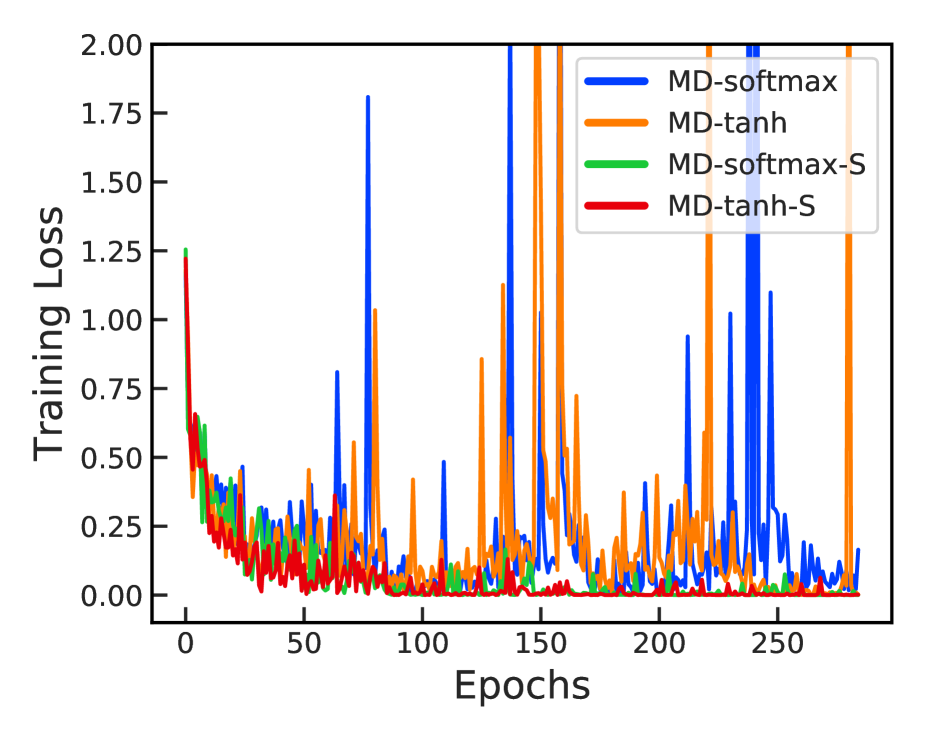
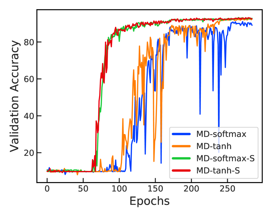
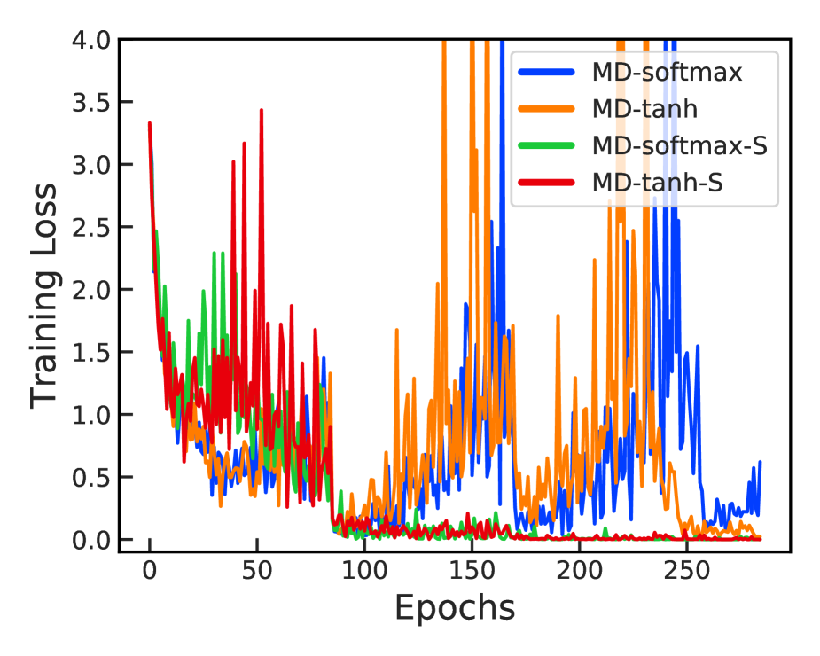
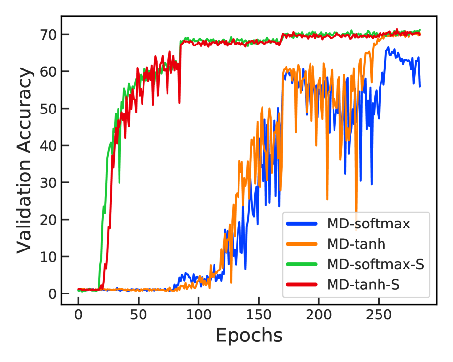
Figure 3: Training curves for binarization for CIFAR-10 (first two) and CIFAR-100 (last two) with ResNet-18. Compared to original md variants, stable md variants are less noisy and after the initial exploration phase (up to $60$ in CIFAR-10 and $25$ epochs CIFAR-100), the validation accuracies rise sharply and show gradual improvement afterwards.

5.1 Full Binarization of Parameters

	Algorithm	CIFAR-10	CIFAR-100
	ref (float)	$93.67$	$73.97$
	bc	$86.84$	$65.04$
Ours	md-$\operatorname{softmax}$-s	$89.71$	$66.40$
	md-$\tanh$-s	89.99	66.63

Table 3: Classification accuracies on the test set for MobileNetV2 where all the parameters are binarized. Our stable md variants significantly outperformed bc while md-$\tanh$-s is slightly better than md-$\operatorname{softmax}$-s.

We evaluate both of our md variants corresponding to $\tanh$ and $\operatorname{softmax}$ projections and their numerically stable counterparts as noted in Eq. (12). The results are compared against parameter quantization methods, namely BinaryConnect (bc) (Courbariaux et al., (2015)), ProxQuant (pq) (Bai et al., (2019)) and Proximal Mean-Field (pmf) (Ajanthan et al., (2019)). In addition, for completeness, we also compare against a standard pgd variant corresponding to the $\tanh$ projection (denoted as gd-$\tanh$), i.e., minimizing $f(\tanh(\tilde{\mathbf{x}}))$ using gradient descent. Note that, numerous techniques have emerged with bc as the workhorse algorithm by relaxing constraints such as the layer-wise scalars (Rastegari et al., (2016)), and similar extensions are straightforward even in our case though our variants perform well even without using layer-wise scalars.

The classification accuracies of binary networks obtained by both variants of our algorithm, namely, md-$\tanh$ and md-$\operatorname{softmax}$, their numerically stable versions (denoted with suffix “-s”) and the baselines bc, pq, pmf, gd-$\tanh$ and the floating point Reference Network (ref) are reported in Table 2. Both the numerically stable md variants consistently produce better or on par results compared to other binarization methods while narrowing the performance gap between binary networks and floating point counterparts to a large extent, on multiple datasets.

Our stable md-variant perform slightly better than md-$\operatorname{softmax}$, whereas for $\tanh$, md updates either perform on par or sometimes even better than numerically stable version of md-$\tanh$. We believe, the main reason for this empirical variation in results for our md variants is due to numerical instability caused by the floating-point arithmetic of logarithm and exponential functions in update steps for md (refer to Table 1). Furthermore, even though our two md-variants, namely md-$\operatorname{softmax}$ and md-$\tanh$ optimize in different spaces, their performance is similar in most cases.

Note, pq (Bai et al., (2019)) does not quantize the fully-connected layers, biases, and shortcut layers. For fair comparison as previously mentioned, we crossvalidate pq with all layers binarized and original pq settings, and report the results denoted as pq and pq * respectively in Table 2. Our md-variants outperform pq consistently on multiple datasets in equivalent experimental settings. This clearly shows that entropic or $\tanh$-based regularization with our annealing scheme is superior to a simple “W” shaped regularizer and emphasizes that md is a suitable framework for quantization. Furthermore, the superior performance of md-$\tanh$ against gd-$\tanh$ and on par or better performance of md-$\operatorname{softmax}$ against pmf for binary quantization empirically validates that md is useful even in a nonconvex stochastic setting. This hypothesis along with our numerically stable form of md can be particularly useful to explore other projections that are useful for quantization and/or network compression in general.

The training curves for our md variants for CIFAR-10 and CIFAR-100 datasets with ResNet-18 are shown in Fig. 3. The original md variants show unstable behaviour during training. Regardless, by storing auxiliary variables, the md updates are demonstrated to be quite stable. This clear distinction between md variants emphasizes the significance of practical considerations while implementing md especially in nn optimization.

To further demonstrate the superiority of md, we tested on a more resource efficient MobileNetV2 (Sandler et al., (2018)) and the results are summarized in Table 3. In short, our md variants are able to fully-binarize MobileNetV2 with minimal loss in accuracy on CIFAR datasets. For more experiments such as training curves comparison to other methods and ternary quantization results please refer to the Appendix B.

	Algorithm	Top-1	Top-5
	ref (float)	$70.61$	$89.40$
	bwn * (Rastegari et al., (2016))	$60.80$	$83.00$
	br (Yin et al., (2018))	$63.20$	$85.10$
	elq (Zhou et al., (2018))	$64.72$	$86.04$
	admm (Leng et al., (2018))	$64.80$	$86.20$
	qn (Yang et al., (2019))	$66.50$	87.03
Ours	md-$\tanh$-s*+	$56.67$	$79.66$
	md-$\tanh$-s*	$65.92$	$86.29$
	md-$\tanh$-s	66.78	$87.01$

Table 4: ImageNet classification accuracies for binary quantization (only parameters) on ResNet-18. Here, * indicates training from scratch and ⁺ indicates full-binarization except the batchnorm parameters. Note md-$\tanh$-s outperforms all other methods setting new state-of-the-art on ImageNet binarization. It might seem that the improvement over qn is marginal, however, qn requires layerwise scalars and pretraining (Yang et al., (2019)), whereas md-$\tanh$-s does not require layerwise scaling and obtains near state-of-the-art results even without pretraining.

Algorithm		Top-1	Top-5
ref (float)		$70.6$	$89.4$
BinaryNet (Hubara et al., (2016))		$42.2$	$67.1$
Dorefa-Net (Zhou et al., (2016))		$52.5$	$76.7$
XNOR-Net (Rastegari et al., (2016))		$51.2$	$73.2$
Bireal-Net (Liu et al., (2018))		$56.4$	$79.5$
Bireal-Net (Liu et al., (2018)) (PReLU)		$59.0$	$81.3$
PCNN (J=1) (Gu et al., (2019))		$57.3$	$80.0$
QN (Yang et al., (2019))		$53.6$	$75.3$
BOP (Helwegen et al., (2019))		$54.2$	$77.2$
GBCN (Liu et al., (2019))		$57.8$	$80.9$
IR-Net (Qin et al., (2020))		$58.1$	$80.0$
Noisy Supervision (Han et al., (2020))		$59.4$	$81.7$
Ours	md-$\tanh$-s	$60.3$	$82.3$
	md-$\tanh$-s (kl div. loss)	62.8	84.3

Table 5: ImageNet classification accuracies for binary quantization (both parameters and activations) on ResNet-18. Here, our md-$\tanh$-s and Han et al., (2020) use Bireal-Net-18 (Liu et al., (2018)) with PReLU activations as baseline architecture. We also show results of our method with kl divergence loss between softmax output of our binary network and ref (trained ResNet-34 on ImageNet). Note, md-$\tanh$-s clearly outperforms all the methods.

5.2 Binarization on ImageNet

We evaluated our md-$\tanh$-s against state-of-the-art methods on ImageNet with ResNet-18 for parameter binarization and the results are reported in Table 4. Following the standard practice, we do not quantize the first convolution layer, last fully-connected layer, biases, and batchnorm parameters for all the compared methods and in this case, we set a new state-of-the-art for binarization with achieving merely $\bf{<4\%}$ reduction compared to the floating-point network. Note that, the standard practice to quantize on ImageNet is to use floating-point scalars in each layer (Rastegari et al., (2016); Yang et al., (2019)), however, our method outperforms all the methods without requiring layerwise scalars. In addition, md-$\tanh$-s yields the best results even when trained from scratch with ${\bf<1\%}$ reduction compared to finetuning from a pretrained network. Furthermore, md enables the training of fully-binarized networks with no additional scalars (except the batchnorm parameters) from scratch, which is considered to be difficult for ImageNet (Rastegari et al., (2016)). More ablation study experiments can be found in Appendix B.

Similar to the above, the results for both parameters and activations binarized networks are reported in Table 5. For this experiment, we use Bireal-Net-18 (Liu et al., (2018)) with PReLU activations as network architecture for our proposed algorithm. Even in this experiment, the first convolution layer, last fully-connected layer, biases, and batchnorm parameters are not binarized for all the methods. Our md-$\tanh$-s achieves state-of-the-art results even when both parameters and activations are binarized, beating all the comparable baselines by almost ${\bf 1\%}$. In addition, similar to Zhuang et al., (2018); Martinez et al., (2019); Liu et al., (2020), we ran md-$\tanh$-s with kl Divergence loss (replacing the cross-entropy loss) between the softmax output of our binary network and ref (trained ResNet-34 on ImageNet). Our md-$\tanh$-s with kl divergence loss outperforms previous methods by a significant margin of ${\bf>3\%}$, which clearly reflects the efficacy of md.

6 Discussion

In this work, we have introduced an md framework for nn quantization by deriving mirror maps corresponding to two projections useful for quantization and provided two algorithms for quantization. Theoretically, we provided a convergence analysis in the convex setting for time-varying mirror maps and discussed conditions to ensure convergence to a discrete solution when an annealing hyperparameter is employed. In addition, we have discussed a numerically stable implementation of md by storing an additional set of auxiliary variables and showed that this update is strikingly analogous to the popular ste based gradient method. The superior performance of our md formulation even with simple projections such as $\tanh$ and $\operatorname{softmax}$ is encouraging and we believe, md would be a suitable framework for not just nn quantization but for network compression in general. In the future, we intend to focus more on the theoretical aspects of md in conjunction with stochastic momentum based optimizers such as Adam.

7 Acknowledgements

This work was supported by the ERC grant ERC-2012-AdG 321162-HELIOS, EPSRC grant Seebibyte EP/M013774/1, EPSRC/MURI grant EP/N019474/1, and the Australian Research Council Centre of Excellence for Robotic Vision (project number CE140100016). We would like to thank Pawan Kumar for useful discussions on mirror descent and we acknowledge the Royal Academy of Engineering, FiveAI, Data61, CSIRO, and National Computing Infrastructure, Australia.

Appendices

Here, we first provide the proofs and the technical derivations. Later we give additional experiments and the details of our experimental setting.

Appendix A md Proofs and Derivations

A.1 More details on Projections

Here, we provide more details on projections used in the paper for nn quantization. Even though we consider differentiable projections, Theorem 1 in the main paper does not require the projection to be differentiable. For the rest of the section, we assume $m=1$, i.e., consider projections that are independent for each ${j\in\{1,\ldots,m\}}$.

Example 1 ($\mathbf{w}$-space, binary, $\tanh$).

Consider the $\tanh$ function, which projects a real value to the interval $[-1,1]$:

$$w=P_{\beta_{k}}(\tilde{w}):=\tanh(\beta_{k}\tilde{w})=\frac{\exp(2\beta_{k}\tilde{w})-1}{\exp(2\beta_{k}\tilde{w})+1}\ ,\vspace{-0.5ex}$$ (14)

where $\beta_{k}\geq 1$ is the annealing hyperparameter and when $\beta_{k}\to\infty$, $\tanh$ approaches the step function. The inverse of the $\tanh$ is:

$$P^{-1}_{\beta_{k}}(w)=\frac{1}{\beta_{k}}\tanh^{-1}(w)=\frac{1}{2\beta_{k}}\log\frac{1+w}{1-w}\ .\vspace{-1ex}$$ (15)

Note that, $P^{-1}_{\beta_{k}}$ is monotonically increasing for a fixed $\beta_{k}$. Correspondingly, the mirror map from Theorem 1 in the main paper can be written as:

$$\Phi_{\beta_{k}}(w) =\int P^{-1}_{\beta_{k}}(w)dw$$

$$=\frac{1}{2\beta_{k}}\big{[}(1+w)\log(1+w)+(1-w)\log(1-w)\big{]}\ .$$ (16)

Here, the constant from the integration is ignored. It can be easily verified that $\Phi_{\beta_{k}}(w)$ is in fact a valid mirror map. Correspondingly, the Bregman divergence can be written as:

$$D_{\Phi_{\beta_{k}}}(w,v) =\Phi_{\beta_{k}}(w)-\Phi_{\beta_{k}}(v)-\Phi^{\prime}_{\beta_{k}}(v)(w-v)\ ,\quad\mbox{where $\Phi_{\beta_{k}}^{\prime}(v)=\frac{1}{2\beta_{k}}\log\frac{1+v}{1-v}$}\ ,$$ (17)

$$=\frac{1}{2\beta_{k}}\left[w\log\frac{(1+w)(1-v)}{(1-w)(1+v)}+\log(1-w)(1+w)-\log(1-v)(1+v)\right]\ .$$

Now, consider the proximal form of md update

$$w^{k+1} ={\underset{\mathbf{x}\in(-1,1)}{\operatorname{argmin}}}\,\langle\eta\,g^{k},w\rangle+D_{\Phi_{\beta_{k}}}(w,w^{k})\ .$$ (18)

The idea is to find $w$ such that the kkt conditions are satisfied. To this end, let us first write the Lagrangian of Eq. (18) by introducing dual variables $y$ and $z$ corresponding to the constraints $w>-1$ and $w<1$, respectively:

$$F(w,x,y) =\eta g^{k}w+y(-w-1)+z(w-1)$$ (19)

$$+\frac{1}{2\beta_{k}}\left[w\log\frac{(1+w)(1-w^{k})}{(1-w)(1+w^{k})}+\log(1-w)(1+w)-\log(1-w^{k})(1+w^{k})\right]\ .$$

Now, setting the derivatives with respect to $w$ to zero:

$$\frac{\partial F}{\partial w} =\eta g^{k}+\frac{1}{2\beta_{k}}\log\frac{(1+w)(1-w^{k})}{(1-w)(1+w^{k})}-y+z=0\ .$$ (20)

From complementary slackness conditions,

$$y(-w-1) =0\ ,\qquad\text{since}\quad w>-1\ \Rightarrow\ y=0\ ,$$ (21)

$$z(w-1) =0\ ,\qquad\text{since}\quad w<1\ \Rightarrow\ z=0\ .$$

Therefore, Eq. (20) now simplifies to:

$$\frac{\partial F}{\partial w} =\eta g^{k}+\frac{1}{2\beta_{k}}\log\frac{(1+w)(1-w^{k})}{(1-w)(1+w^{k})}=0\ ,$$ (22)

$$\log\frac{(1+w)(1-w^{k})}{(1-w)(1+w^{k})} =-2\beta_{k}\eta g^{k}\ ,$$

$$\frac{1+w}{1-w} =\frac{1+w^{k}}{1-w^{k}}\exp(-2\beta_{k}\eta g^{k})\ ,$$

$$w =\frac{\frac{1+w^{k}}{1-w^{k}}\exp(-2\beta_{k}\eta g^{k})-1}{\frac{1+w^{k}}{1-w^{k}}\exp(-2\beta_{k}\eta g^{k})+1}\ .$$

A similar derivation can also be performed for the $\operatorname{sigmoid}$ function, where $\bar{\mathcal{C}}=\mathcal{X}=[0,1]$. Note that the $\operatorname{sign}$ function has been used for binary quantization in Courbariaux et al., (2015) and $\tanh$ can be used as a soft version of $\operatorname{sign}$ function as pointed out by Zhang et al., (2015). Mirror map corresponding to $\tanh$ is used for online linear optimization in Bubeck et al., (2012) but here we use it for nn quantization. The pseudocodes of original (md-$\tanh$) and numerically stable versions (md-$\tanh$-s) for $\tanh$ are presented in Algorithms 1 and 2 respectively.

Algorithm 1 md-$\tanh$

1:$K,b,\{\eta^{k}\},\rho>1,\mathcal{D},L$

2:$\mathbf{w}^{*}\in\mathcal{Q}^{m}$

3:$\mathbf{w}^{0}\in\rm I\!R^{m},\quad\beta_{0}\leftarrow 1$ $\triangleright$ Initialization

4:$\mathbf{w}^{0}\leftarrow\tanh({\beta_{0}\mathbf{w}^{0}})$ $\triangleright$ Projection

5:for $k\leftarrow 0,\ldots,K$ do

6:     $\mathcal{D}^{b}=\{\left(\mathbf{x}_{i},\mathbf{y}_{i}\right)\}^{b}_{i=1}\sim\mathcal{D}$ $\triangleright$ Sample a mini-batch

7:     $\mathbf{g}^{k}\leftarrow\left.\nabla_{\mathbf{w}}L(\mathbf{w};\mathcal{D}^{b})\right|_{\mathbf{w}=\mathbf{w}^{k}}$ $\triangleright$ Gradient w.r.t. $\mathbf{w}$ at $\mathbf{w}^{k}$ (Adam based gradients)

8:     for $j\leftarrow{1,\ldots,m}$ do

9:         $w_{j}^{k+1}\leftarrow\frac{\frac{1+w_{j}^{k}}{1-w_{j}^{k}}\exp(-2\beta_{k}\eta^{k}g_{j}^{k})-1}{\frac{1+w_{j}^{k}}{1-w_{j}^{k}}\exp(-2\beta_{k}\eta^{k}g_{j}^{k})+1}$ $\triangleright$ md update

10:     end for

11:     $\beta_{k+1}\leftarrow\rho\beta_{k}$ $\triangleright$ Increase $\beta$

12:end for

13:$\mathbf{w}^{*}\leftarrow\operatorname{sign}({\tilde{\mathbf{w}}^{K}})$ $\triangleright$ Quantization

Algorithm 2 md-$\tanh$-s

1:$K,b,\{\eta^{k}\},\rho>1,\mathcal{D},L$

2:$\mathbf{w}^{*}\in\mathcal{Q}^{m}$

3:$\tilde{\mathbf{w}}^{0}\in\rm I\!R^{m},\quad\beta_{0}\leftarrow 1$ $\triangleright$ Initialization

4:for $k\leftarrow 0,\ldots,K$ do

5:     $\mathbf{w}^{k}\leftarrow\tanh({\beta_{k}\tilde{\mathbf{w}}^{k}})$ $\triangleright$ Projection

6:     $\mathcal{D}^{b}=\{\left(\mathbf{x}_{i},\mathbf{y}_{i}\right)\}^{b}_{i=1}\sim\mathcal{D}$ $\triangleright$ Sample a mini-batch

7:     $\mathbf{g}^{k}\leftarrow\left.\nabla_{\mathbf{w}}L(\mathbf{w};\mathcal{D}^{b})\right|_{\mathbf{w}=\mathbf{w}^{k}}$ $\triangleright$ Gradient w.r.t. $\mathbf{w}$ at $\mathbf{w}^{k}$ (Adam based gradients)

8:     $\tilde{\mathbf{w}}^{k+1}\leftarrow\tilde{\mathbf{w}}^{k}-\eta^{k}\mathbf{g}^{k}$ $\triangleright$ Gradient descent on $\tilde{\mathbf{w}}$

9:     $\beta_{k+1}\leftarrow\rho\beta_{k}$ $\triangleright$ Increase $\beta$

10:end for

11:$\mathbf{w}^{*}\leftarrow\operatorname{sign}({\tilde{\mathbf{w}}^{K}})$ $\triangleright$ Quantization

Example 2 ($\mathbf{u}$-space, multi-label, $\operatorname{softmax}$).

Now we consider the $\operatorname{softmax}$ projection used in pmf (Ajanthan et al., (2019)) to optimize in the lifted probability space. In this case, the projection is defined as $P_{\beta_{k}}(\tilde{\mathbf{u}}):=\operatorname{softmax}(\beta_{k}\tilde{\mathbf{u}})$ where $P_{\beta_{k}}:\rm I\!R^{d}\to\mathcal{C}$ with $\bar{\mathcal{C}}=\mathcal{X}=\Delta$. Here $\Delta$ is the $(d-1)$-dimensional probability simplex and $|\mathcal{Q}|=d$. Note that the $\operatorname{softmax}$ projection is not invertible as it is a many-to-one mapping. In particular, it is invariant to translation, i.e.,

$$\mathbf{u}=\operatorname{softmax}(\tilde{\mathbf{u}}+c\bm{1})=\operatorname{softmax}(\tilde{\mathbf{u}})\ ,$$

$$\text{where}\quad u_{\lambda}=\frac{\exp(\tilde{u}_{\lambda})}{\sum_{\mu\in\mathcal{Q}}\exp(\tilde{u}_{\mu})}\ ,\vspace{-0.5ex}$$

for any scalar $c\in\rm I\!R$ ($\bm{1}$ denotes a vector of all ones). Therefore, the $\operatorname{softmax}$ projection does not satisfy Theorem 1 in the main paper. However, one could obtain a solution of the inverse of $\operatorname{softmax}$ as follows: given $\mathbf{u}\in\Delta$, find a unique point $\tilde{\mathbf{v}}=\tilde{\mathbf{u}}+c\bm{1}$, for a particular scalar $c$, such that $\mathbf{u}=\operatorname{softmax}(\tilde{\mathbf{v}})$. Now, by choosing $c=-\log(\sum_{\mu=\mathcal{Q}}\exp(\tilde{u}_{\mu}))$, $\operatorname{softmax}$ can be written as:

$$\mathbf{u}=\operatorname{softmax}(\tilde{\mathbf{v}})\ ,\qquad\text{where}\quad u_{\lambda}=\exp(\tilde{v}_{\lambda})\ ,\quad\forall\,\lambda\in\mathcal{Q}\ .\vspace{-1ex}$$ (23)

Now, the inverse of the projection $P_{\beta_{k}}$ can be written as:

$$\tilde{\mathbf{v}}=P^{-1}_{\beta_{k}}(\mathbf{u})=\frac{1}{\beta_{k}}\operatorname{softmax}^{-1}(\mathbf{u})\ ,\qquad\text{where}\quad\tilde{v}_{\lambda}=\frac{1}{\beta_{k}}\log(u_{\lambda})\ ,\qquad\forall\,\lambda\ .\vspace{-1ex}$$ (24)

Indeed, $\log$ is a monotonically increasing function and from Theorem 1 in the main paper, by summing the integrals, the mirror map can be written as:

$$\Phi_{\beta_{k}}(\mathbf{u})=\frac{1}{\beta_{k}}\left[\sum_{\lambda}u_{\lambda}\log(u_{\lambda})-u_{\lambda}\right]=-\frac{1}{\beta_{k}}H(\mathbf{u})-1/\beta_{k}\ .\vspace{-1ex}$$ (25)

Here, $\sum_{\lambda}u_{\lambda}=1$ as $\mathbf{u}\in\Delta$, and $H(\mathbf{u})$ is the entropy. Interestingly, as the mirror map in this case is the negative entropy (up to a constant), the md update leads to the well-known Exponentiated Gradient Descent (egd) (or eda) (Beck and Teboulle, (2003); Bubeck, (2015)). Consequently, the update takes the following form:

$$u^{k+1}_{\lambda} =\frac{u_{\lambda}^{k}\,\exp(-\beta_{k}\eta g^{k}_{\lambda})}{\sum_{\mu\in\mathcal{Q}}\;u_{\mu}^{k}\,\exp(-\beta_{k}\eta g^{k}_{\mu})}\quad\forall\,\lambda\ .$$ (26)

The derivation follows the same approach as in the $\tanh$ case above. It is interesting to note that the md variant of $\operatorname{softmax}$ is equivalent to the well-known egd. Notice, the authors of pmf (Ajanthan et al., (2019)) hinted that pmf is related to egd but here we have clearly showed that the md variant of pmf under the above reparametrization (23) is exactly egd.

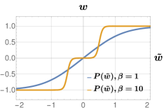
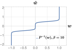
Figure 4: Plots of shifted $\tanh$ projections, and their inverses corresponding to the $\tanh$ projection. Note that, the inverse is monotonically increasing. Moreover, when $\beta_{k}\to\infty$, the projections approaches their respective hard versions.

Example 3 ($\mathbf{w}$-space, multi-label, shifted $\tanh$).

Note that, similar to $\operatorname{softmax}$, we wish to extend the $\tanh$ projection beyond binary. The idea is to use a function that is an addition of multiple shifted $\tanh$ functions. To this end, as an example we consider ternary quantization, with $\mathcal{Q}=\{-1,0,1\}$ and define our shifted $\tanh$ projection $P_{\beta_{k}}:\rm I\!R\to\mathcal{C}$ as:

$$w=P_{\beta_{k}}(\tilde{w})=\frac{1}{2}\big{[}\tanh\left(\beta_{k}(\tilde{w}+0.5)\right)+\tanh\left(\beta_{k}(\tilde{w}-0.5)\right)\big{]}\ ,$$ (27)

where $\beta_{k}\geq 1$ and $w=\bar{\mathcal{C}}=\mathcal{X}=[-1,1]$. When $\beta_{k}\to\infty$, $P_{\beta_{k}}$ approaches a stepwise function with inflection points at $-0.5$ and $0.5$ (here, $\pm 0.5$ is chosen heuristically), meaning $w$ move towards one of the quantization levels in the set $\mathcal{Q}$.

This behaviour together with its inverse is illustrated in Fig. 4. Now, one could potentially find the functional form of $P^{-1}_{\beta_{k}}$ and analytically derive the mirror map corresponding to this projection. Note that, while Theorem 1 in the main paper provides an analytical method to derive mirror maps, in some cases such as the above, the exact form of mirror map and the md update might be nontrivial. In such cases, as shown in the paper, the md update can be easily implemented by storing an additional set of auxiliary variables $\tilde{w}$.

A.2 Convergence Proof for md with Adaptive Mirror Maps

Theorem 3.

Let $\mathcal{X}\subset\rm I\!R^{r}$ be a convex compact set and $\mathcal{C}\subset\rm I\!R^{r}$ be a convex open set with $\mathcal{X}\cap\mathcal{C}\neq\emptyset$ and $\mathcal{X}\subset\bar{\mathcal{C}}$. Let $\Phi:\mathcal{C}\to\rm I\!R$ be a mirror map $\rho$-strongly convex on $\mathcal{X}\cap\mathcal{C}$ with respect to $\left\lVert\cdot\right\rVert$, $R^{2}=\sup_{\mathbf{x}\in\mathcal{X}\cap\mathcal{C}}\Phi(\mathbf{x})-\Phi(\mathbf{x}^{0})$ where $\mathbf{x}^{0}=\operatorname*{argmin}_{\mathbf{x}\in\mathcal{X}\cap\mathcal{C}}\Phi(\mathbf{x})$ is the initialization, and $f:\mathcal{X}\to\rm I\!R$ be a convex function and $L$-Lipschitz with respect to $\left\lVert\cdot\right\rVert$. Then md with mirror map $\Phi_{\beta_{k}}(\mathbf{x})=\Phi(\mathbf{x})/\beta_{k}$ with $1\leq\beta_{k}\leq B$ and $\eta=\frac{R}{L}\sqrt{\frac{2\rho}{Bt}}$ satisfies

$$f\left(\frac{1}{t}\sum_{k=0}^{t-1}\mathbf{x}^{k}\right)-f(\mathbf{x}^{*})\leq RL\sqrt{\frac{2B}{\rho t}}\ ,$$ (28)

where $\beta_{k}$ is the annealing hyperparameter, $\eta>0$ is the learning rate, $t$ is the iteration index, and $\mathbf{x}^{*}$ is the optimal solution.

Proof.

The proof is a slight modification to the proof of standard md and we refer the reader to the proof of Theorem 4.2 of Bubeck, (2015) for step by step derivation. We first discuss the intuition and then turn to the detailed proof. For the standard md the bound is:

$$f\left(\frac{1}{t}\sum_{k=0}^{t-1}\mathbf{x}^{k}\right)-f(\mathbf{x}^{*})\leq RL\sqrt{\frac{2}{\rho t}}\ ,$$ (29)

with $\eta=\frac{R}{L}\sqrt{\frac{2\rho}{t}}$. Here, since $\beta_{k}\leq B$, the adaptive mirror map ${\Phi_{\beta_{k}}(\mathbf{x})=\Phi(\mathbf{x})/\beta_{k}}$ is $\rho/B$-strongly convex for all $k$. Therefore, by simply replacing $\rho$ with $\rho/B$ the desired bound is obtained.

We now provide the step-by-step derivation for completeness. First note the md update with the adaptive mirror map:

$$\nabla\Phi_{\beta_{k}}(\mathbf{y}^{k+1}) =\nabla\Phi_{\beta_{k}}(\mathbf{x}^{k})-\eta\mathbf{g}^{k}\ ,\quad\mbox{where $\mathbf{g}^{k}\in\partial f(\mathbf{x}^{k})$ and $\mathbf{y}^{k+1}\in\mathcal{C}$}\ ,$$ (30)

$$\mathbf{g}^{k} =(\nabla\Phi_{\beta_{k}}(\mathbf{x}^{k})-\nabla\Phi_{\beta_{k}}(\mathbf{y}^{k+1}))/\eta,\quad\mbox{$\eta>0$}\ .$$

Now, let $\mathbf{x}\in\mathcal{X}\cap\mathcal{C}$. The claimed bound will be obtained by taking a limit $\mathbf{x}\to\mathbf{x}^{*}$.

$$f(\mathbf{x}^{k})-f(\mathbf{x}) \leq\langle\mathbf{g}^{k},\mathbf{x}^{k}-\mathbf{x}\rangle\ ,\quad\mbox{$f$ is convex}\ ,$$ (31)

$$=\langle\nabla\Phi_{\beta_{k}}(\mathbf{x}^{k})-\nabla\Phi_{\beta_{k}}(\mathbf{y}^{k+1}),\mathbf{x}^{k}-\mathbf{x}\rangle/\eta\ ,\quad\mbox{Eq.~{}(\ref{eq:amd1})}\ ,$$

$$=\left(D_{\Phi_{\beta_{k}}}(\mathbf{x},\mathbf{x}^{k})+D_{\Phi_{\beta_{k}}}(\mathbf{x}^{k},\mathbf{y}^{k+1})-D_{\Phi_{\beta_{k}}}(\mathbf{x},\mathbf{y}^{k+1})\right)/\eta\ ,\quad\mbox{Bregman div.}\ ,$$

$$\leq\left(D_{\Phi_{\beta_{k}}}(\mathbf{x},\mathbf{x}^{k})+D_{\Phi_{\beta_{k}}}(\mathbf{x}^{k},\mathbf{y}^{k+1})-D_{\Phi_{\beta_{k}}}(\mathbf{x},\mathbf{x}^{k+1})-D_{\Phi_{\beta_{k}}}(\mathbf{x}^{k+1},\mathbf{y}^{k+1})\right)/\eta\ .$$

The last line is due to the inequality ${D_{\Phi_{\beta_{k}}}(\mathbf{x},\mathbf{x}^{k+1})+D_{\Phi_{\beta_{k}}}(\mathbf{x}^{k+1},\mathbf{y}^{k+1})\geq D_{\Phi_{\beta_{k}}}(\mathbf{x},\mathbf{y}^{k+1})}$, where $\mathbf{x}^{k+1}=\operatorname*{argmin}_{\mathbf{x}\in\mathcal{X}\cap\mathcal{C}}\,D_{\Phi_{\beta_{k}}}(\mathbf{x},\mathbf{y}^{k+1})$. Notice that,

$$\sum_{k=0}^{t-1}D_{\Phi_{\beta_{k}}}(\mathbf{x},\mathbf{x}^{k})-D_{\Phi_{\beta_{k}}}(\mathbf{x},\mathbf{x}^{k+1}) =\sum_{k=0}^{t-1}\left(D_{\Phi}(\mathbf{x},\mathbf{x}^{k})-D_{\Phi}(\mathbf{x},\mathbf{x}^{k+1})\right)/\beta_{k}\ ,$$ (32)

$$=\beta_{0}^{-1}\big{(}D_{\Phi}(\mathbf{x},\mathbf{x}^{0})-D_{\Phi}(\mathbf{x},\mathbf{x}^{1})\big{)}+\beta_{1}^{-1}\big{(}D_{\Phi}(\mathbf{x},\mathbf{x}^{1})-D_{\Phi}(\mathbf{x},\mathbf{x}^{2})\big{)}+\ldots+$$

$$\qquad\beta_{t-1}^{-1}\big{(}D_{\Phi}(\mathbf{x},\mathbf{x}^{t-1})-D_{\Phi}(\mathbf{x},\mathbf{x}^{t})\big{)},$$

$$=\beta_{0}^{-1}D_{\Phi}(\mathbf{x},\mathbf{x}^{0})+(\beta_{1}^{-1}-\beta_{0}^{-1})D_{\Phi}(\mathbf{x},\mathbf{x}^{1})+\ldots+(\beta_{t-1}^{-1}-\beta_{t-2}^{-1})D_{\Phi}(\mathbf{x},\mathbf{x}^{t-1})-$$

$$\qquad\beta_{t-1}^{-1}D_{\Phi}(\mathbf{x},\mathbf{x}^{t}),$$

$$\leq\beta_{0}^{-1}D_{\Phi}(\mathbf{x},\mathbf{x}^{0}),\qquad\mbox{$D_{\Phi}(\mathbf{x},\mathbf{z})\geq 0,\ \forall\,\mathbf{x},\mathbf{z}\in\mathcal{C}$ and $\beta_{k+1}^{-1}-\beta_{k}^{-1}<0,\forall\,k$}\,$$

$$\leq D_{\Phi}(\mathbf{x},\mathbf{x}^{0}),\qquad\mbox{$\beta_{0}\geq 1$}\,$$

Now we bound the remaining term:

$$D_{\Phi_{\beta_{k}}}(\mathbf{x}^{k},\mathbf{y}^{k+1})-D_{\Phi_{\beta_{k}}}(\mathbf{x}^{k+1},\mathbf{y}^{k+1})$$ (33)

$$=\Phi_{\beta_{k}}(\mathbf{x}^{k})-\Phi_{\beta_{k}}(\mathbf{x}^{k+1})-\langle\nabla\Phi_{\beta_{k}}(\mathbf{y}^{k+1}),\mathbf{x}^{k}-\mathbf{x}^{k+1}\rangle\ ,\quad\mbox{Bregman divergence def.}\ ,$$

$$\leq\langle\nabla\Phi_{\beta_{k}}(\mathbf{x}^{k})-\nabla\Phi_{\beta_{k}}(\mathbf{y}^{k+1}),\mathbf{x}^{k}-\mathbf{x}^{k+1}\rangle-\frac{\rho}{2\beta_{k}}\left\lVert\mathbf{x}^{k}-\mathbf{x}^{k+1}\right\rVert^{2}\ ,\quad\mbox{$\Phi$ is $\rho$-strongly convex}\ ,$$

$$=\langle\eta\mathbf{g}^{k},\mathbf{x}^{k}-\mathbf{x}^{k+1}\rangle-\frac{\rho}{2\beta_{k}}\left\lVert\mathbf{x}^{k}-\mathbf{x}^{k+1}\right\rVert^{2}\ ,\quad\mbox{Eq.~{}(\ref{eq:amd1})}\ ,$$

$$\leq\eta L(\mathbf{x}^{k}-\mathbf{x}^{k+1})-\frac{\rho}{2\beta_{k}}\left\lVert\mathbf{x}^{k}-\mathbf{x}^{k+1}\right\rVert^{2}\ ,\quad\mbox{$f$ is $L$-Lipschitz}\ ,$$

$$\leq\frac{(\eta L)^{2}\beta_{k}}{2\rho}\ ,\qquad\mbox{$az-bz^{2}\leq a^{2}/(4b),\ \forall\,z\in\rm I\!R$}\ ,$$

$$\leq\frac{(\eta L)^{2}B}{2\rho}\ ,\qquad\mbox{$\beta_{k}\leq B$}\ .$$

Putting Eqs. (32) and (33) in Eq. (31),

$$\frac{1}{t}\sum_{k=0}^{t-1}\left(f(\mathbf{x}^{k})-f(\mathbf{x})\right) \leq\frac{D_{\Phi}(\mathbf{x},\mathbf{x}^{0})}{\eta t}+\frac{\eta BL^{2}}{2\rho}\ ,$$ (34)

$$f\left(\frac{1}{t}\sum_{k=0}^{t-1}\mathbf{x}^{k}\right)-f(\mathbf{x}) \leq\frac{R^{2}}{\eta t}+\frac{\eta BL^{2}}{2\rho}\ ,\quad\mbox{Jensen inequality, defs. of $\mathbf{x}^{0}$ and $R$}\ ,$$

$$=RL\sqrt{\frac{2B}{\rho t}}\ ,\quad\mbox{Substituting $\eta=\frac{R}{L}\sqrt{\frac{2\rho}{Bt}}$}\ .$$

Note the additional multiplication by $\sqrt{B}$ compared to the standard md bound. However, the convergence rate is still $\mathcal{O}(1/\sqrt{t})$. ∎

A.3 Proof for Epsilon Convergence to a Discrete Solution via Annealing

Proposition 2.

For a given $B>0$ and $0<\epsilon<1$, there exists a $\gamma>0$ such that if $|\tilde{x}|\geq\gamma$ then ${1-|\tanh(B\tilde{x})|<\epsilon}$. Here $|\cdot|$ denotes the absolute value and $\gamma>\tanh^{-1}(1-\epsilon)/B$.

Proof.

For a given $B$ and $\epsilon$, we derive a condition on $|\tilde{x}|$ for the inequality to be satisfied.

$$1-|\tanh(B\tilde{x})| <\epsilon\ ,$$ (35)

$$|\tanh(B\tilde{x})| >1-\epsilon\ ,$$ (36)

$$\tanh(B|\tilde{x}|) >1-\epsilon\ ,\quad\mbox{$|\tanh(\tilde{x})|=\tanh(|\tilde{x}|)$}$$ (37)

$$|\tilde{x}| >\tanh^{-1}(1-\epsilon)/B\ .\quad\mbox{$\tanh$ is monotone}$$ (38)

Therefore for any $\gamma>\tanh^{-1}(1-\epsilon)/B$, the above inequality is satisfied. ∎

Appendix B Additional Experiments

We first give training curves of all compared methods, provide ablation study of ImageNet experiments as well as ternary quantization results as a proof of concept. Later, we provide experimental details.

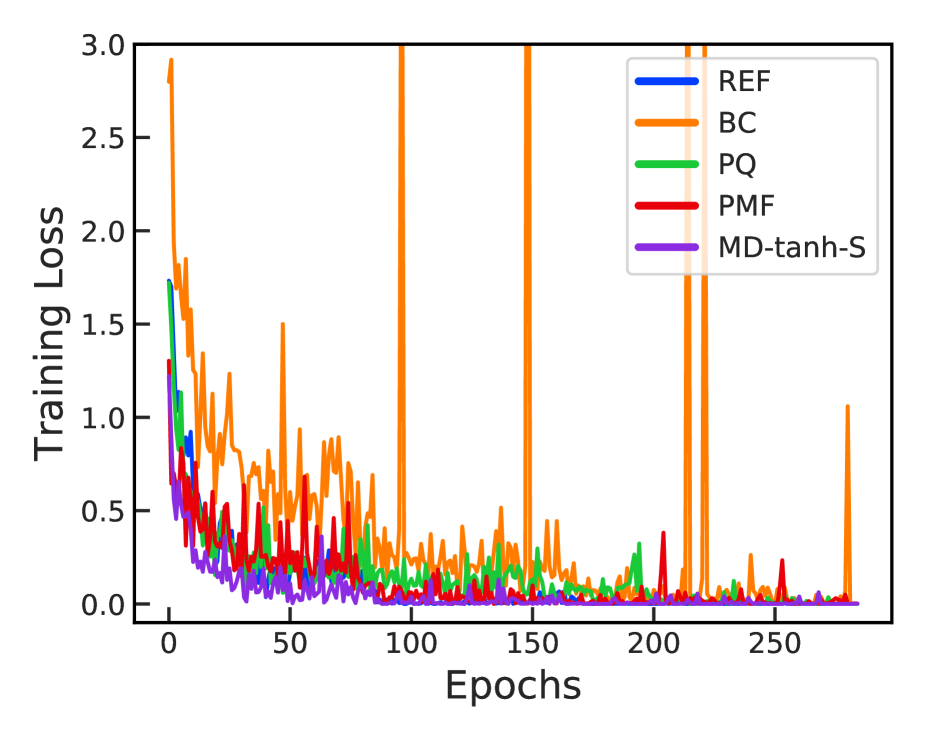
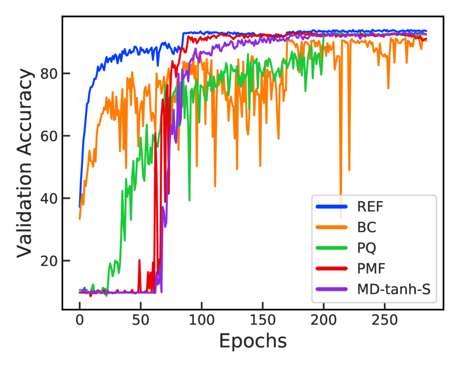
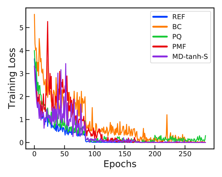
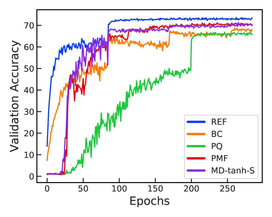
Figure 5: Training curves for binarization for CIFAR-10 (first two columns) and CIFAR-100 (last two columns) with ResNet-18. Compared to bc, our md-$\tanh$-s and pmf are less noisy and after the initial exploration phase (up to $60$ in CIFAR-10 and $25$ epochs CIFAR-100), the validation accuracies rise sharply and closely resembles the floating point network afterwards. This steep increase is not observed in regularization methods such as pq.

B.1 Convergence Analysis

The training curves for CIFAR-10 and CIFAR-100 datasets with ResNet-18 are shown in Fig. 5. Notice, after the initial exploration phase (due to low $\beta$) the validation accuracies of our md-$\tanh$-s increase sharply while this steep rise is not observed in regularization methods such as pq. The training behaviour for both our stable md-variants ($\operatorname{softmax}$ and $\tanh$) is quite similar.

B.2 ImageNet Ablation Study

	Pretrained	Conv1 and fc	Bias	bn	Layerwise Scaling	Accuracy
md-$\tanh$-s	✓	Float	Float	Float	✗	66.78/87.01
	✗	Float	Float	Float	✗	$65.92/86.29$
	✓	Binary	Float	Float	✗	$60.39/82.77$
	✗	Binary	Float	Float	✗	$59.92/82.42$
	✓	Binary	Binary	Float	✗	$56.60/79.79$
	✗	Binary	Binary	Float	✗	$56.67/79.66$
	✓	Binary	Float	Float	✓	$61.91/83.87$
	✓	Binary	Binary	Float	✓	$56.05/79.69$

Table 6: Ablation study on ImageNet with ResNet-18 for weights binarization using md-$\tanh$-s. While the best performance is obtained for the case where Conv1, fc and biases are not quantized, md-$\tanh$-s obtains good performance even when fully-quantized regardless of either using a pretrained network or training from scratch.

We provide an ablation study for various experimental settings for weights binarization on ImageNet dataset using ResNet-18 architecture in Table 6. We perform experiments for both training for scratch and pretrained networks with variation in binarization of first convolution layer, fully connected layer and biases. Note that the performance degradation of our binary networks is minimal on all layers binarized network except biases using simple layerwise scaling as mentioned in McDonnell, (2018). Contrary to the standard setup of binarized network training for ImageNet, where first and last layers are kept floating point, our md-$\tanh$-s method achieves good performance even on the fully-quantized network irrespective of either using a pretrained network or network trained from scratch.

	Algorithm	Space	CIFAR-10		CIFAR-100		TinyImageNet
			VGG-16	ResNet-18	VGG-16	ResNet-18	ResNet-18
	ref (float)	$\mathbf{w}$	$93.33$	$94.84$	$71.50$	$76.31$	$58.35$
	pq	$\mathbf{w}$	$83.32$	$90.50$	$32.16$	$59.18$	$41.46$
	pq *	$\mathbf{w}$	92.20	93.85	$57.64$	$70.98$	$45.72$
	gd-$\tanh$	$\mathbf{w}$	$91.21$	$93.20$	$53.88$	$69.48$	$50.65$
Ours	md-$\operatorname{softmax}$-s	$\mathbf{u}$	$91.69$	$93.30$	$65.11$	72.01	$52.21$
	md-$\tanh$-s	$\mathbf{w}$	$91.70$	$93.42$	66.15	$71.29$	52.69

Table 7: Classification accuracies on the test set for ternary quantization. pq * denotes performance with fully-connected layers, first convolution layer, and shortcut layers in floating point whereas pq represent results with all layers quantized. Also, pq * optimize for the quantization levels as well (different for each layer), in contrast we fix it to $\mathcal{Q}=\{-1,0,1\}$. gd-$\tanh$ denotes results without using ste and actually calculating the gradient through the projection.

B.3 Ternary Quantization Results

As a proof of concept for our shifted $\tanh$ projection (refer Example 3), we also show results for ternary quantization with quantization levels ${\mathcal{Q}=\{-1,0,1\}}$ in Table 7. Note that the performance improvement of our ternary networks compared to their respective binary networks is marginal as only $0$ is included as the $3^{\text{rd}}$ quantization level. In contrast to us, the baseline method pq (Bai et al., (2019)) optimizes for the quantization levels (differently for each layer) as well in an alternating optimization regime rather than fixing it to $\mathcal{Q}=\{-1,0,1\}$. Also, pq does ternarize the first convolution layer, fully-connected layers and the shortcut layers. We crossvalidate hyperparameters for both the original pq setup and the equivalent setting of our md-variants where we optimize all the weights and denote them as pq * and pq respectively.

Our md-$\tanh$ variant performs on par or sometimes even better in comparison to $\tanh$ projection results where gradient is calculated through the projection instead of performing md. This again empirically validates the hypothesis that md yields in good approximation for the task of network quantization. The better performance of pq in their original quantization setup, compared to our approach in CIFAR-10 can be accounted to their non-quantized layers and different quantization levels. We believe similar explorations are possible with our md framework as well.

Dataset	Image	# class	Train / Val.	$b$	$K$
CIFAR-10	$32\times 32$	$10$	$45$k / $5$k	$128$	$100$k
CIFAR-100	$32\times 32$	$100$	$45$k / $5$k	$128$	$100$k
TinyImageNet	$64\times 64$	$200$	$100$k / $10$k	$128$	$100$k
ImageNet	$224\times 224$	$1000$	$1.2$M / $50$k	$2048/256$	$90/55$

Table 8: Experiment setup. Here, $b$ is the batch size and $K$ is the total number of iterations for all datasets except ImageNet where $K$ indicates number of epochs for training from scratch and pretrained network respectively. For ImageNet, $b$ represents batch size for training from scratch and pretrained networks respectively.

Hyperparameters	Fine-tuning grid
learning_rate	$[0.1,0.01,0.001,0.0001]$
lr_scale	$[0.1,0.2,0.3,0.5]$
beta_scale	$[1.01,1.02,1.05,1.1,1.2]$
beta_scale_interval	$[100,200,500,1000,2000]$

Table 9: The hyperparameter search space for all the experiments. Chosen parameters are given in Tables 10, 11 and 12.

B.4 Experimental Details

As mentioned in the main paper the experimental protocol is similar to Ajanthan et al., (2019). To this end, the details of the datasets and their corresponding experiment setups are given in Table 8. For CIFAR-10/100 and TinyImageNet, VGG-16 (Simonyan and Zisserman, (2015)), ResNet-18 (He et al., (2016)) and MobileNetV2 (Sandler et al., (2018)) architectures adapted for CIFAR dataset are used. In particular, for CIFAR experiments, similar to Lee et al., (2019), the size of the fully-connected (fc) layers of VGG-16 is set to $512$ and no dropout layers are employed. For TinyImageNet, the stride of the first convolutional layer of ResNet-18 is set to $2$ to handle the image size (Huang et al., (2017)). In all the models, batch normalization (Ioffe and Szegedy, (2015)) (with no learnable parameters) and ReLU nonlinearity are used. Only for the floating point networks (i.e., ref), we keep the learnable parameters for batch norm. Standard data augmentation (i.e., random crop and horizontal flip) is used.

For both of our md variants, hyperparameters such as the learning rate, learning rate scale, annealing hyperparameter $\beta$ and its schedule are crossvalidated from the range reported in Table 9 and the chosen parameters are given in the Table 10, Table 11 and Table 12. To generate the plots, we used the publicly available codes of bc , pq and pmf .

All methods are trained from a random initialization and the model with the best validation accuracy is chosen for each method. Note that, in md, even though we use an increasing schedule for $\beta$ to enforce a discrete solution, the chosen network may not be fully-quantized (as the best model could be obtained in an early stage of training). Therefore, simple $\operatorname*{argmax}{}$ rounding is applied to ensure that the network is fully-quantized.

	CIFAR-10 with ResNet-18
	md-$\operatorname{softmax}$	md-$\tanh$	md-$\operatorname{softmax}$-s	md-$\tanh$-s	pmf *	gd-$\tanh$	bc	pq
learning_rate	0.001	0.001	0.001	0.001	0.001	0.001	0.001	0.01
lr_scale	0.2	0.3	0.3	0.3	0.3	0.3	0.3	0.5
beta_scale	1.02	1.01	1.02	1.02	1.1	1.1	-	0.0001
beta_scale_interval	200	100	200	200	1000	1000	-	-
	CIFAR-100 with ResNet-18
	md-$\operatorname{softmax}$	md-$\tanh$	md-$\operatorname{softmax}$-s	md-$\tanh$-s	pmf *	gd-$\tanh$	bc	pq
learning_rate	0.001	0.001	0.001	0.001	0.001	0.001	0.001	0.1
lr_scale	0.2	0.3	0.2	0.2	0.3	0.5	0.2	-
beta_scale	1.05	1.05	1.1	1.2	1.01	1.01	-	0.001
beta_scale_interval	500	500	200	500	100	100	-	-
	CIFAR-10 with VGG-16
	md-$\operatorname{softmax}$	md-$\tanh$	md-$\operatorname{softmax}$-s	md-$\tanh$-s	pmf *	gd-$\tanh$	bc	pq
learning_rate	0.01	0.001	0.001	0.001	0.001	0.001	0.0001	0.01
lr_scale	0.2	0.3	0.3	0.2	0.5	0.3	0.3	0.5
beta_scale	1.05	1.1	1.2	1.2	1.05	1.1	-	0.0001
beta_scale_interval	500	1000	2000	2000	500	1000	-	-
	CIFAR-100 with VGG-16
	md-$\operatorname{softmax}$	md-$\tanh$	md-$\operatorname{softmax}$-s	md-$\tanh$-s	pmf *	gd-$\tanh$	bc	pq
learning_rate	0.001	0.001	0.0001	0.001	0.0001	0.001	0.0001	0.01
lr_scale	0.3	0.3	0.2	0.5	0.5	0.5	0.2	0.5
beta_scale	1.01	1.05	1.2	1.05	1.02	1.1	-	0.0001
beta_scale_interval	100	500	500	500	200	1000	-	-
	TinyImageNet with ResNet-18
	md-$\operatorname{softmax}$	md-$\tanh$	md-$\operatorname{softmax}$-s	md-$\tanh$-s	pmf *	gd-$\tanh$	bc	pq
learning_rate	0.001	0.001	0.001	0.001	0.001	0.001	0.001	0.01
lr_scale	0.2	0.5	0.1	0.1	0.5	0.5	0.5	-
beta_scale	1.02	1.2	1.02	1.2	1.01	1.01	-	0.0001
beta_scale_interval	200	2000	100	500	100	100	-	-

Table 10: Hyperparameter settings used for the binary quantization experiments. Here, the learning rate is multiplied by lr_scale after every 30k iterations and annealing hyperparameter $(\beta)$ is multiplied by beta_scale after every beta_scale_interval iterations. We use Adam optimizer with zero weight decay. For pq, beta_scale denotes regularization rate.

	CIFAR-10 with ResNet-18
	ref (float)	md-$\operatorname{softmax}$-s	md-$\tanh$-s	gd-$\tanh$	pq	pq *
learning_rate	0.1	0.001	0.01	0.01	0.01	0.01
lr_scale	0.3	0.3	0.2	0.5	0.3	-
beta_scale	-	1.05	1.2	1.02	0.0001	0.0001
beta_scale_interval	-	500	1000	500	-	-
weight_decay	0.0001	0	0	0	0	0.0001
	CIFAR-100 with ResNet-18
	ref (float)	md-$\operatorname{softmax}$-s	md-$\tanh$-s	gd-$\tanh$	pq	pq *
learning_rate	0.1	0.001	0.001	0.01	0.01	0.001
lr_scale	0.1	0.1	0.5	0.5	0.2	-
beta_scale	-	1.1	1.1	1.02	0.0001	0.0001
beta_scale_interval	-	100	500	1000	-	-
weight_decay	0.0001	0	0	0	0	0.0001
	CIFAR-10 with VGG-16
	ref (float)	md-$\operatorname{softmax}$-s	md-$\tanh$-s	gd-$\tanh$	pq	pq *
learning_rate	0.1	0.001	0.01	0.01	0.01	0.1
lr_scale	0.2	0.3	0.3	0.3	-	-
beta_scale	-	1.05	1.1	1.01	1e-07	0.0001
beta_scale_interval	-	500	1000	500	-	-
weight_decay	0.0001	0	0	0	0	0.0001
	CIFAR-100 with VGG-16
	ref (float)	md-$\operatorname{softmax}$-s	md-$\tanh$-s	gd-$\tanh$	pq	pq *
learning_rate	0.1	0.0001	0.001	0.01	0.01	0.0001
lr_scale	0.2	0.3	0.5	0.2	-	-
beta_scale	-	1.05	1.1	1.05	0.0001	0.0001
beta_scale_interval	-	100	500	2000	-	-
weight_decay	0.0001	0	0	0	0	0.0001
	TinyImageNet with ResNet-18
	ref (float)	md-$\operatorname{softmax}$-s	md-$\tanh$-s	gd-$\tanh$	pq	pq *
learning_rate	0.1	0.001	0.01	0.01	0.01	0.01
lr_scale	0.1	0.1	0.1	0.5	-	-
beta_scale	-	1.2	1.2	1.05	0.01	0.0001
beta_scale_interval	-	500	2000	2000	-	-
weight_decay	0.0001	0	0	0	0	0.0001

Table 11: Hyperparameter settings used for the ternary quantization experiments. Here, the learning rate is multiplied by lr_scale after every 30k iterations and annealing hyperparameter $(\beta)$ is multiplied by beta_scale after every beta_scale_interval iterations. We use Adam optimizer except for ref for which sgd with momentum $0.9$ is used. For pq, beta_scale denotes regularization rate.

	CIFAR-10 with MobileNet-V2
	ref (float)	bc	md-$\operatorname{softmax}$-s	md-$\tanh$-s
learning_rate	0.01	0.001	0.01	0.01
lr_scale	0.5	0.5	0.3	0.2
beta_scale	-	-	1.1	1.2
beta_scale_interval	-	-	1000	2000
weight_decay	0.0001	0	0	0
	CIFAR-100 with MobileNet-V2
	ref (float)	bc	md-$\operatorname{softmax}$-s	md-$\tanh$-s
learning_rate	0.01	0.001	0.01	0.01
lr_scale	0.5	0.2	0.1	0.1
beta_scale	-	-	1.1	1.02
beta_scale_interval	-	-	500	100
weight_decay	0.0001	0	0	0

Table 12: Hyperparameter settings used for the binary quantization experiments. Here, the learning rate is multiplied by lr_scale after every 30k iterations and annealing hyperparameter $(\beta)$ is multiplied by beta_scale after every beta_scale_interval iterations. We use Adam optimizer except for ref for which sgd with momentum $0.9$ is used.

	ImageNet with ResNet-18
	ref (float)	md-$\tanh$-s*	md-$\tanh$-s
base_learning_rate	2.048	2.048	0.0768
warmup_epochs	8	8	0
beta_scale	-	1.02	1.02
beta_scale_interval (iterations)	-	62	275
batch_size	2048	2048	256
weight_decay	3.0517e-05	3.0517e-05	3.0517e-05

Table 13: Hyperparameter settings used for the binary quantization experiments on ImageNet dataset using ResNet-18 architecture. Here md-$\tanh$-s* is trained from scratch while md-$\tanh$-s is finetuned on the pretrained network. We use sgd optimizer with momentum $0.875$ and cosine learning rate scheduler for all experiments. For all the experiments, weight decay in batchnorm layers are off. Similar to Goyal et al., (2017), for experiments with larger batch size we use gradual warmup where learning rate is linearly scaled from small learning rate to the base learning rate. Also, note that training schedule is fixed based on above hyperparameters for ablation study on ImageNet dataset.

B.5 ImageNet

We use the standard ResNet-18 architecture for ImageNet experiments where we train for $90$ epochs and $55$ epochs for training from scratch and pretrained network respectively. We perform all ImageNet experiments using NVIDIA DGX-1 machine with $8$ Tesla V-100 GPUs for training from scratch and single Tesla V-100 GPU for training from a pretrained network. We provide detailed hyperparameter setup used for our experiments in Table 13. Similar to experiments on the other datasets, to enforce a discrete solution simple rounding based on $\operatorname{sign}$ operation is applied to ensure that the final network is fully-quantized. The final accuracy is reported based on the $\operatorname{sign}$ operation based discrete model obtained at the end of the final epoch.

References

- Achterhold et al., (2018) Achterhold, J., Kohler, J. M., Schmeink, A., and Genewein, T. (2018). Variational network quantization. ICLR.
- Ajanthan et al., (2019) Ajanthan, T., Dokania, P. K., Hartley, R., and Torr, P. H. (2019). Proximal mean-field for neural network quantization. ICCV.
- Bai et al., (2019) Bai, Y., Wang, Y.-X., and Liberty, E. (2019). Proxquant: Quantized neural networks via proximal operators. ICLR.
- Beck and Teboulle, (2003) Beck, A. and Teboulle, M. (2003). Mirror descent and nonlinear projected subgradient methods for convex optimization. Operations Research Letters.
- Boyd and Vandenberghe, (2009) Boyd, S. and Vandenberghe, L. (2009). Convex optimization. Cambridge university press.
- Bubeck, (2015) Bubeck, S. (2015). Convex optimization: Algorithms and complexity. Foundations and Trends® in Machine Learning.
- Bubeck et al., (2012) Bubeck, S., Cesa-Bianchi, N., and Kakade, S. M. (2012). Towards minimax policies for online linear optimization with bandit feedback. Conference on Learning Theory.
- Carreira-Perpinán and Idelbayev, (2017) Carreira-Perpinán, M. A. and Idelbayev, Y. (2017). Model compression as constrained optimization, with application to neural nets. part ii: Quantization. NeurIPS Workshop on Optimization for Machine Learning.
- Chen et al., (2019) Chen, S., Wang, W., and Pan, S. J. (2019). MetaQuant: learning to quantize by learning to penetrate non-differentiable quantization. NeurIPS.
- Courbariaux et al., (2015) Courbariaux, M., Bengio, Y., and David, J.-P. (2015). Binaryconnect: Training deep neural networks with binary weights during propagations. NeurIPS.
- Esser et al., (2015) Esser, S. K., Appuswamy, R., Merolla, P. A., Arthur, J. V., and Modha, D. S. (2015). Backpropagation for energy-efficient neuromorphic computing. NeurIPS.
- Goyal et al., (2017) Goyal, P., Dollár, P., Girshick, R., Noordhuis, P., Wesolowski, L., Kyrola, A., Tulloch, A., Jia, Y., and He, K. (2017). Accurate, large minibatch sgd: Training imagenet in 1 hour. arXiv preprint arXiv:1706.02677.
- Gu et al., (2019) Gu, J., Li, C., Zhang, B., Han, J., Cao, X., Liu, J., and Doermann, D. (2019). Projection convolutional neural networks for 1-bit cnns via discrete back propagation. AAAI.
- Guo, (2018) Guo, Y. (2018). A survey on methods and theories of quantized neural networks. arXiv preprint arXiv:1808.04752.
- Han et al., (2020) Han, K., Wang, Y., Xu, Y., Xu, C., Wu, E., and Xu, C. (2020). Training binary neural networks through learning with noisy supervision. ICML.
- He et al., (2016) He, K., Zhang, X., Ren, S., and Sun, J. (2016). Deep residual learning for image recognition. CVPR.
- Helwegen et al., (2019) Helwegen, K., Widdicombe, J., Geiger, L., Liu, Z., Cheng, K.-T., and Nusselder, R. (2019). Latent weights do not exist: Rethinking binarized neural network optimization. NeurIPS.
- Hou et al., (2017) Hou, L., Yao, Q., and Kwok, J. T. (2017). Loss-aware binarization of deep networks. ICLR.
- Hsieh et al., (2018) Hsieh, Y.-P., Kavis, A., Rolland, P., and Cevher, V. (2018). Mirrored langevin dynamics. NeurIPS.
- Huang et al., (2017) Huang, G., Li, Y., Pleiss, G., Liu, Z., Hopcroft, J. E., and Weinberger, K. Q. (2017). Snapshot ensembles: Train 1, get m for free. ICLR.
- Hubara et al., (2016) Hubara, I., Courbariaux, M., Soudry, D., El-Yaniv, R., and Bengio, Y. (2016). Binarized neural networks. NeurIPS.
- Hubara et al., (2017) Hubara, I., Courbariaux, M., Soudry, D., El-Yaniv, R., and Bengio, Y. (2017). Quantized neural networks: Training neural networks with low precision weights and activations. JMLR.
- Ioffe and Szegedy, (2015) Ioffe, S. and Szegedy, C. (2015). Batch normalization: Accelerating deep network training by reducing internal covariate shift. ICML.
- Lee et al., (2019) Lee, N., Ajanthan, T., and Torr, P. H. S. (2019). SNIP: Single-shot network pruning based on connection sensitivity. ICLR.
- Leng et al., (2018) Leng, C., Dou, Z., Li, H., Zhu, S., and Jin, R. (2018). Extremely low bit neural network: Squeeze the last bit out with ADMM. AAAI.
- Li et al., (2017) Li, H., De, S., Xu, Z., Studer, C., Samet, H., and Goldstein, T. (2017). Training quantized nets: A deeper understanding. NeurIPS.
- Liu et al., (2019) Liu, C., Ding, W., Hu, Y., Zhang, B., Liu, J., and Guo, G. (2019). Gbcns: Genetic binary convolutional networks for enhancing the performance of 1-bit dcnns. CoRR.
- Liu et al., (2020) Liu, Z., Shen, Z., Savvides, M., and Cheng, K.-T. (2020). Reactnet: Towards precise binary neural network with generalized activation functions. arXiv preprint arXiv:2003.03488.
- Liu et al., (2018) Liu, Z., Wu, B., Luo, W., Yang, X., Liu, W., and Cheng, K.-T. (2018). Bi-real net: Enhancing the performance of 1-bit cnns with improved representational capability and advanced training algorithm. ECCV.
- Louizos et al., (2019) Louizos, C., Reisser, M., Blankevoort, T., Gavves, E., and Welling, M. (2019). Relaxed quantization for discretized neural networks. ICLR.
- Louizos et al., (2017) Louizos, C., Ullrich, K., and Welling, M. (2017). Bayesian compression for deep learning. NeurIPS.
- Martinez et al., (2019) Martinez, B., Yang, J., Bulat, A., and Tzimiropoulos, G. (2019). Training binary neural networks with real-to-binary convolutions. In International Conference on Learning Representations.
- McDonnell, (2018) McDonnell, M. D. (2018). Training wide residual networks for deployment using a single bit for each weight. ICLR.
- McMahan, (2017) McMahan, H. B. (2017). A survey of algorithms and analysis for adaptive online learning. JMLR.
- Nemirovsky and Yudin, (1983) Nemirovsky, A. S. and Yudin, D. B. (1983). Problem complexity and method efficiency in optimization.
- Paszke et al., (2017) Paszke, A., Gross, S., Chintala, S., Chanan, G., Yang, E., DeVito, Z., Lin, Z., Desmaison, A., Antiga, L., and Lerer, A. (2017). Automatic differentiation in PyTorch.
- Qin et al., (2020) Qin, H., Gong, R., Liu, X., Shen, M., Wei, Z., Yu, F., and Song, J. (2020). Forward and backward information retention for accurate binary neural networks. CVPR.
- Rastegari et al., (2016) Rastegari, M., Ordonez, V., Redmon, J., and Farhadi, A. (2016). Xnor-net: Imagenet classification using binary convolutional neural networks. ECCV.
- Sandler et al., (2018) Sandler, M., Howard, A., Zhu, M., Zhmoginov, A., and Chen, L.-C. (2018). Mobilenetv2: inverted residuals and linear bottlenecks. CVPR.
- Simonyan and Zisserman, (2015) Simonyan, K. and Zisserman, A. (2015). Very deep convolutional networks for large-scale image recognition. ICLR.
- Yang et al., (2019) Yang, J., Shen, X., Xing, J., Tian, X., Li, H., Deng, B., Huang, J., and Hua, X.-s. (2019). Quantization networks. CVPR.
- Ye et al., (2019) Ye, S., Feng, X., Zhang, T., Ma, X., Lin, S., Li, Z., Xu, K., Wen, W., Liu, S., Tang, J., et al. (2019). Progressive dnn compression: A key to achieve ultra-high weight pruning and quantization rates using admm. arXiv preprint arXiv:1903.09769.
- Yin et al., (2019) Yin, P., Lyu, J., Zhang, S., Osher, S., Qi, Y., and Xin, J. (2019). Understanding straight-through estimator in training activation quantized neural nets. ICLR.
- Yin et al., (2018) Yin, P., Zhang, S., Lyu, J., Osher, S., Qi, Y., and Xin, J. (2018). Binaryrelax: A relaxation approach for training deep neural networks with quantized weights. SIIMS.
- Zhang et al., (2015) Zhang, R., Lin, L., Zhang, R., Zuo, W., and Zhang, L. (2015). Bit-scalable deep hashing with regularized similarity learning for image retrieval and person re-identification. TIP.
- Zhang and He, (2018) Zhang, S. and He, N. (2018). On the convergence rate of stochastic mirror descent for nonsmooth nonconvex optimization. CoRR.
- Zhou et al., (2018) Zhou, A., Yao, A., Wang, K., and Chen, Y. (2018). Explicit loss-error-aware quantization for low-bit deep neural networks. CVPR.
- Zhou et al., (2016) Zhou, S., Wu, Y., Ni, Z., Zhou, X., Wen, H., and Zou, Y. (2016). Dorefa-net: Training low bitwidth convolutional neural networks with low bitwidth gradients. CoRR.
- (49) Zhou, Z., Mertikopoulos, P., Bambos, N., Boyd, S., and Glynn, P. (2017a). Mirror descent in non-convex stochastic programming. CoRR.
- (50) Zhou, Z., Mertikopoulos, P., Bambos, N., Boyd, S., and Glynn, P. W. (2017b). Stochastic mirror descent in variationally coherent optimization problems. NeurIPS.
- Zhuang et al., (2018) Zhuang, B., Shen, C., Tan, M., Liu, L., and Reid, I. (2018). Towards effective low-bitwidth convolutional neural networks. In Proceedings of the IEEE conference on computer vision and pattern recognition, pages 7920–7928.