Deterministic generation of Greenberger-Horne-Zeilinger entangled states of cat-state qubits in circuit QED

Abstract

We present an efficient method to generate a Greenberger-Horne-Zeilinger (GHZ) entangled state of three cat-state qubits (cqubits) via circuit QED. The GHZ state is prepared with three microwave cavities coupled to a superconducting transmon qutrit. Because the qutrit remains in the ground state during the operation, decoherence caused by the energy relaxation and dephasing of the qutrit is greatly suppressed. The GHZ state is created deterministically because no measurement is involved. Numerical simulations show that high-fidelity generation of a three-cqubit GHZ state is feasible with present circuit QED technology. This proposal can be easily extended to create a $N$-cqubit GHZ state ($N\geq 3$), with $N$ microwave or optical cavities coupled to a natural or artificial three-level atom.

Cat-state qubits (cqubits), encoded with cat states, have drawn intensive attention due to their enhanced life times s1 . Recently, there is an increasing interest in quantum computing with cqubits. Schemes have been presented for realizing single-cqubit gates and two-cqubit gates s2 ; s3 ; s4 . Moreover, single-cqubit gates s5 and two-cqubit entangled Bell states s6 have been experimentally demonstrated. On the other hand, circuit QED, consisting of microwave cavities and superconducting qubits or qutrits, has been considered as one of the leading candidates for quantum information processing (for reviews, see s7 ; s8 ; s9 ).

The goal of this letter focuses on generation of Greenberger-Horne-Zeilinger (GHZ) entangled states of cqubits via circuit QED. GHZ states have many important applications in quantum information processing s10 , quantum communication s11 , and high-precision spectroscopy s12 . We will propose an efficient method to create three-cqubit GHZ states, by using three microwave cavities coupled to a superconducting transmon qutrit (a three-level artificial atom) [Fig. 1(a)].

This proposal has the following advantages. During the state preparation, the qutrit stays in the ground state. Thus, decoherence from the qutrit is greatly suppressed. The GHZ state is deterministically created because this proposal does not require any measurement on the state of the coupler qutrit or the state of the cqubits. Numerical simulations show that high-fidelity creation of a three-cqubit GHZ state is feasible with current circuit QED technology. This proposal can be easily extended to generate a $N$-cqubit GHZ state ($N\geq 3$), with $N$ microwave or optical cavities coupled to a natural or artificial three-level atom. To the best of our knowledge, this work is the first to demonstrate generation of GHZ entangled states with cqubits.

The three levels of the transmon qutrit are denoted as $|g\rangle$, $|e\rangle$ and $|f\rangle$ [Fig. 1(b)]. The $|g\rangle$ $\leftrightarrow$ $|f\rangle$ coupling for a transmon qutrit is forbidden or weak s13 . Cavity $1$ is off-resonantly coupled to the $|g\rangle\leftrightarrow|e\rangle$ transition of the qutrit but highly detuned (decoupled) from the $|e\rangle\leftrightarrow|f\rangle$ transition of the qutrit. In addition, cavity $l$ ($l=2,3$) is off-resonantly coupled to the $|e\rangle\leftrightarrow|f\rangle$ transition of the qutrit but highly detuned (decoupled) from the $|g\rangle\leftrightarrow|e\rangle$ transition of the qutrit (Fig. 2). These conditions can in principle be satisfied by prior adjustment of the qutrit’s level spacings or the cavity frequency. For a superconducting qutrit, the level spacings can be rapidly (within 1-3 ns) adjusted s14 ; s15 . In addition, the frequency of a microwave cavity can be quickly tuned in $1\sim 2$ ns s16 ; s17 .

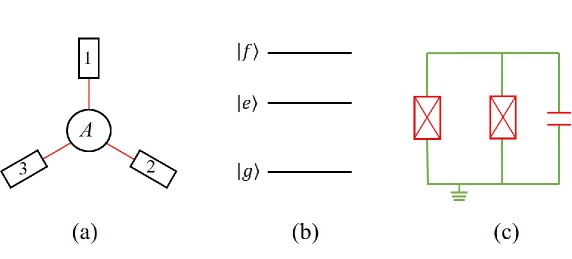
Figure 1: (Color online) (a) Diagram of three cavities coupled to a transmon qutrit (labelled by $A$). Each square represents a cavity, which can be a one- or three-dimensional cavity. The qutrit is capacitively or inductively coupled to each cavity. (b) Level configuration of the transmon qutrit, whose level spacing between the upper two levels is smaller than that between the two lowest levels. (c) Circuit of a transmon qutrit, which consists of two Josephson junctions and a capacitor.

Under the above assumptions, the Hamiltonian, in the interaction picture and after making the rotating-wave approximation, can be written as (in units of $\hbar=1$)

$$H_{\mathrm{I}}=g_{1}(e^{i\left|\delta_{1}\right|t}\hat{a}_{1}^{+}\sigma_{eg}^{-}+h.c.)+\sum\limits_{l=2}^{3}g_{l}(e^{-i\left|\delta_{l}\right|t}\hat{a}_{l}^{+}\sigma_{fe}^{-}+h.c.),$$ (1)

where $g_{1}$ and $g_{l}$ are the coupling constants, $\left|\delta_{1}\right|=\omega_{c_{1}}-\omega_{eg},$ $\left|\delta_{l}\right|=\omega_{fe}-\omega_{c_{l}},$ $\sigma_{eg}^{-}=|g\rangle\langle e|$, $\sigma_{fe}^{-}=|e\rangle\langle f|$. The detunings $\left|\delta_{1}\right|$ and $\left|\delta_{l}\right|$ have a relationship $\left|\delta_{l}\right|=\left|\delta_{1}\right|+\Delta_{1l},$ with $\Delta_{1l}=\omega_{fg}-\omega_{c_{1}}-\omega_{c_{l}}>0$ (Fig. 2). Here, $\hat{a}_{1}^{+}$ ($\hat{a}_{l}^{+}$) is the photon creation operator of cavity $1$ ($l$), $\omega_{c_{1}}$ ($\omega_{c_{l}}$) is the frequency of cavity $1$ ($l$ ($l=2,3$)); while $\omega_{fe},$ $\omega_{eg},$ and $\omega_{fg}$ are the $|e\rangle\leftrightarrow|f\rangle,$ $|g\rangle\leftrightarrow|e\rangle,$ and $|g\rangle\leftrightarrow|f\rangle$ transition frequencies of the qutrit, respectively.

Under the large-detuning conditions $\left|\delta_{1}\right|\gg g_{1}$ and $\left|\delta_{l}\right|\gg g_{l}$, the Hamiltonian (1) becomes s18

$$H_{\mathrm{e},1}= \lambda_{1}(\hat{a}_{1}^{+}\hat{a}_{1}|g\rangle\langle g|-\hat{a}_{1}\hat{a}_{1}^{+}|e\rangle\langle e|)$$

$$-\sum\limits_{l=2}^{3}\lambda_{l}(\hat{a}_{l}^{+}\hat{a}_{l}|e\rangle\langle e|-\hat{a}_{l}\hat{a}_{l}^{+}|f\rangle\langle f|)$$

$$+\lambda_{23}\left(e^{i\bigtriangleup_{23}t}\hat{a}_{2}^{+}\hat{a}_{3}+h.c.\right)\left(|f\rangle\langle f|-|e\rangle\langle e|\right)$$

$$+\sum\limits_{l=2}^{3}\lambda_{1l}(e^{-i\bigtriangleup_{1l}t}\hat{a}_{1}^{+}\hat{a}_{l}^{+}\sigma_{fg}^{-}+h.c.),$$ (2)

where $\lambda_{1}=g_{1}^{2}/\left|\delta_{1}\right|$, $\lambda_{l}=g_{l}^{2}/\left|\delta_{l}\right|$, $\lambda_{1l}=\left(g_{1}g_{l}/2\right)(1/|\delta_{1}|+1/|\delta_{l}|)$, $\lambda_{23}=\left(g_{2}g_{3}/2\right)(1/|\delta_{2}|+1/|\delta_{3}|),$ $\bigtriangleup_{23}=\left|\delta_{3}\right|-|\delta_{2}|$ $=\omega_{c_{2}}-\omega_{c_{3}},$ and $\sigma_{fg}^{-}=|g\rangle\langle f|$. In Eq. (2), the terms in the first two lines describe the photon number dependent stark shifts of the energy levels $|g\rangle$, $|e\rangle$ and $|f\rangle$; the terms in the third line describe the coupling between cavities $2$ and 3; while the terms in the last line describe the $|f\rangle$ $\leftrightarrow$ $|g\rangle$ coupling, caused due to the cooperation of cavities $1$ and $l$ ($l=2,3$).

For $\bigtriangleup_{1l}\gg\{\lambda_{1},\lambda_{l},\lambda_{23},\lambda_{1l}\}$, the Hamiltonian $H_{\mathrm{e},1}$ changes to s18

$$H_{\mathrm{e},2}= \lambda_{1}(\hat{a}_{1}^{+}\hat{a}_{1}|g\rangle\langle g|-\hat{a}_{1}\hat{a}_{1}^{+}|e\rangle\langle e|)$$

$$-\sum\limits_{l=2}^{3}\lambda_{l}(\hat{a}_{l}^{+}\hat{a}_{l}|e\rangle\langle e|-\hat{a}_{l}\hat{a}_{l}^{+}|f\rangle\langle f|)$$

$$+\lambda_{23}\left(e^{i\bigtriangleup_{23}t}\hat{a}_{2}^{+}\hat{a}_{3}+h.c.\right)\left(|f\rangle\langle f|-|e\rangle\langle e|\right)$$

$$+\sum\limits_{l=2}^{3}\chi_{1l}(\hat{a}_{1}\hat{a}_{1}^{+}\hat{a}_{l}\hat{a}_{l}^{+}|f\rangle\langle f|-\hat{a}_{1}^{+}\hat{a}_{1}\hat{a}_{l}^{+}\hat{a}_{l}|g\rangle\langle g|),$$ (3)

where $\chi_{1l}=\lambda_{1l}^{2}/\Delta_{1l}$. When the levels $|e\rangle$ and $|f\rangle$ are initially not occupied, they will remain unpopulated, because both $|g\rangle\rightarrow|e\rangle$ and $|g\rangle\rightarrow|f\rangle$ transitions are not induced by the Hamiltonian (3). Thus, the Hamiltonian (3) becomes $H_{\mathrm{e},3}=\lambda_{1}\hat{n}_{1}|g\rangle\langle g|-\sum\limits_{l=2}^{n}\chi_{1l}\hat{n}_{1}\hat{n}_{l}|g\rangle\langle g|,$ where $\hat{n}_{1}=\hat{a}_{1}^{+}\hat{a}_{1}$ ($\hat{n}_{l}=\hat{a}_{l}^{+}\hat{a}_{l}$) is the photon number operators for cavities $1$ ($l$).

Suppose that the qutrit is initially in the ground state $\left|g\right\rangle$. It will remain in this state throughout the interaction, as the Hamiltonian $H_{\mathrm{e},3}$ cannot induce any transition for the qutrit. In this case, the Hamiltonian $H_{\mathrm{e},3}$ is reduced to

$$H_{\mathrm{e}}=\lambda_{1}\hat{n}_{1}-\sum\limits_{l=2}^{3}\chi_{1l}\hat{n}_{1}\hat{n}_{l},$$ (4)

which is the effective Hamiltonian governing the dynamics of the three cavities.

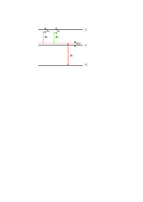
Figure 2: (Color online) Cavity $1$ is far-off resonant with the $|g\rangle\leftrightarrow|e\rangle$ transition with coupling strength $g_{1}$ and detuning $\left|\delta_{1}\right|$, while cavity $l$ ($l=2,3$) is far-off resonant with the $|e\rangle\leftrightarrow|f\rangle$ transition with coupling strength $g_{l}$ and detuning $\left|\delta_{l}\right|$. Here, $\left|\delta_{l}\right|$ ($l=2,3$) is not drawn to simplify the figure. $\left|\delta_{1}\right|=\omega_{c_{1}}-\omega_{eg}$, $\left|\delta_{l}\right|=\omega_{fe}-\omega_{c_{l}}=\left|\delta_{1}\right|+\Delta_{1l},$ and $\Delta_{1l}=\omega_{fg}-\omega_{c_{1}}-\omega_{c_{l}}>0$, with frequency $\omega_{c_{1}}$ ($\omega_{c_{l}}$) of cavity $1$ ($l$). The red line represents $\omega_{c_{1}}$, while the brown and green lines represent $\omega_{c_{2}}$ and $\omega_{c_{3}}$, respectively.

The unitary operator $U=e^{-i{H}_{\mathrm{e}}t}$ can be written as $U=U_{1}\otimes\prod\limits_{l=2}^{3}U_{1l},$ where $U_{1}$ is a unitary operator on cavity $1,$ while $U_{1l}$ is a unitary operator on cavities $1$ and $l,$ given by

$$U_{1}=\exp\left(-i\lambda_{1}\hat{n}_{1}t\right),~{}U_{1l}=\exp\left(i\chi_{1l}\hat{n}_{1}\hat{n}_{l}t\right).$$ (5)

The two logical states $|0\rangle$ and $|1\rangle$ of a $cqubit$ are encoded with cat states of a cavity, i.e., $|0\rangle=N_{\alpha}^{+}(|\alpha\rangle+|-\alpha\rangle)$ and $|1\rangle=N_{\alpha}^{-}(|\alpha\rangle-|-\alpha\rangle),$ where $N_{\alpha}^{\pm}$ are the normalization coefficients. Because of $|\alpha\rangle=e^{-|\alpha|^{2}/2}\sum\limits_{n=0}^{\infty}\frac{\alpha^{n}}{\sqrt{n!}}|n\rangle$ and $|-\alpha\rangle=e^{-|\alpha|^{2}/2}\sum\limits_{n=0}^{\infty}\frac{(-\alpha)^{n}}{\sqrt{n!}}|n\rangle,$ one has

$$|0\rangle=\sum\limits_{m=0}^{\infty}C_{2m}|2m\rangle,\text{ }|1\rangle=\sum\limits_{n=0}^{\infty}C_{2n+1}|2n+1\rangle,$$ (6)

where $n$ and $m$ are non-negative integers, $C_{2m}=2N_{\alpha}^{+}e^{-|\alpha|^{2}/2}\alpha^{2m}/\sqrt{(2m)!},$ and $C_{2n+1}=$ $2N_{\alpha}^{-}e^{-|\alpha|^{2}/2}\alpha^{2n+1}/\sqrt{(2n+1)!}$. Eq. (6) shows that the cat state $|0\rangle$ is orthogonal to the cat state $|1\rangle$, independent of $\alpha$ (except for $\alpha=0$).

For $\chi_{1l}t=\pi,$ the unitary operator $U_{1l}$ leads to the following state transformation

$$U_{1l}|2m\rangle_{1}|2m^{\prime}\rangle_{l} =|2m\rangle_{1}|2m^{\prime}\rangle_{l},$$

$$U_{1l}|2m\rangle_{1}|2n^{\prime}+1\rangle_{l} =|2m\rangle_{1}|2n^{\prime}+1\rangle_{l},$$

$$U_{1l}|2n+1\rangle_{1}|2m^{\prime}\rangle_{l} =|2n+1\rangle_{1}|2m^{\prime}\rangle_{l},$$

$$U_{1l}|2n+1\rangle_{1}|2n^{\prime}+1\rangle_{l} =-|2n+1\rangle_{1}|2n^{\prime}+1\rangle_{l},$$ (7)

where we have applied $\exp\left[i(2m)(2m^{\prime})\chi_{1l}t\right]=\exp[i(2m)(2n^{\prime}+1)\chi_{1l}t]=\exp[i(2n+1)(2m^{\prime})\chi_{1l}t]=1$ but $\exp[i(2n+1)(2n^{\prime}+1)\chi_{1l}t]=-1.$ By means of Eq. (7) and according to Eq. (6), it is easy to find the following results

$$U_{1l}|00\rangle_{1l} =|00\rangle_{1l},\text{ }U_{1l}|01\rangle_{1l}=|01\rangle_{1l},$$

$$U_{1l}|10\rangle_{1l} =|10\rangle_{1l},\text{ }U_{1l}|11\rangle_{1l}=-|11\rangle_{1l},$$ (8)

which shows that a phase flip happens to the state $|1\rangle$ of cqubit $l$ when cqubit $1$ is in the state $\left|1\right\rangle$.

The unitary operator $U_{1}$ leads to

$$U_{1}|0\rangle_{1} = \sum\limits_{m=0}^{\infty}\exp\left[i(2m)\lambda_{1}t\right]C_{2m}|2m\rangle_{1},$$

$$U_{1}|1\rangle_{1} = \sum\limits_{n=0}^{\infty}\exp[i(2n+1)\lambda_{1}t]C_{2n+1}|2n+1\rangle_{1}.$$ (9)

For $\lambda_{1}t=2\pi,$ we have $\exp\left[i(2m)\lambda_{1}t\right]=\exp[i(2n+1)\lambda_{1}t]=1.$ Hence, Eq. (9) becomes

$$U_{1}|0\rangle_{1}=|0\rangle_{1},\text{ }U_{1}|1\rangle_{1}=|1\rangle_{1}.$$ (10)

Now assume that the three cqubits are initially in the state $|\psi\rangle_{\mathrm{cq}}=\prod\limits_{l=1}^{3}\frac{1}{\sqrt{2}}\left(\left|0\right\rangle_{l}+\left|1\right\rangle_{l}\right)$, which can be prepared from the state $\prod\limits_{l=1}^{3}\left|0\right\rangle_{l},$ by applying a driving pulse to cavity $l$ to obtain the state rotation $\left|0\right\rangle_{l}\rightarrow\frac{1}{\sqrt{2}}\left(\left|0\right\rangle_{l}+\left|1\right\rangle_{l}\right)$ ($l=1,2,3$) [2]. Based on the results (8) and (10) and according to the expression (6) of the states $|0\rangle$ and $|1\rangle$ and $U=U_{1}\otimes\prod_{l=2}^{3}U_{1l}$, it is straightforward to show that for $t=\pi/\chi_{1l}=2\pi/\lambda_{1},$ the unitary operator $U$ transforms the initial state $|\psi\rangle_{\mathrm{cq}}$ of three cqubits as follows

$$\frac{1}{2\sqrt{2}}\left[\left|0_{1}\right\rangle\left(\left|0_{2}\right\rangle+\left|1_{2}\right\rangle\right)\left(\left|0_{3}\right\rangle+\left|1_{3}\right\rangle\right)\right.$$

$$+\left.\left|1_{1}\right\rangle\left(\left|0_{2}\right\rangle-\left|1_{2}\right\rangle\right)\left(\left|0_{3}\right\rangle-\left|1_{3}\right\rangle\right)\right].$$ (11)

The state (11) can be converted into the following three-cqubit GHZ entangled state

$$\frac{1}{\sqrt{2}}\left(\left|0_{1}\right\rangle\left|0_{2}\right\rangle\left|0_{3}\right\rangle+\left|1_{1}\right\rangle\left|1_{2}\right\rangle\left|1_{3}\right\rangle\right),$$ (12)

by applying a driving pulse to cavity $l$ to achieve the single-cqubit state transformation $\frac{1}{\sqrt{2}}\left(\left|0_{l}\right\rangle+\left|1_{l}\right\rangle\right)\rightarrow\left|0_{l}\right\rangle$ and $\frac{1}{\sqrt{2}}\left(\left|0_{l}\right\rangle-\left|1_{l}\right\rangle\right)\rightarrow\left|1_{l}\right\rangle$ ($l=2,3$) [2].

The above description shows that the coupler qutrit remains in the ground state during the entire operation. Therefore, decoherence from the qutrit is greatly suppressed.

The above condition $\chi_{1l}t=\pi$ and $\lambda_{1}t=2\pi$ turns out into $\chi_{1l}=\lambda_{1}/2$, resulting in

$$g_{l}=\frac{\left|\delta_{l}\right|}{\left|\delta_{1}\right|+\left|\delta_{l}\right|}\sqrt{2\Delta_{1l}\left|\delta_{1}\right|}.$$ (13)

The coupling strength $g_{l}$ can be adjusted by a prior design of the sample with appropriate capacitance or inductance between the qutrit and cavity $l$ s19 .

We now give a brief discussion on the experimental feasibility. Assume that the single-cqubit operation can be performed within a very short time. Thus, the decoherence effect is negligible during the single-cqubit operation and not considered in our numerical simulation for simplicity.

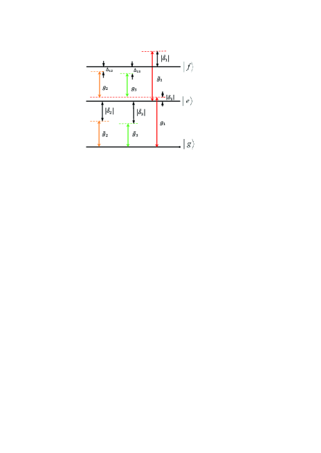
Figure 3: (Color online) Illustration of the unwanted coupling between cavity $1$ and the $|e\rangle\leftrightarrow|f\rangle$ transition with coupling strength $\widetilde{g}_{1}$ and detuning $\left|\widetilde{\delta}_{1}\right|$, as well as the unwanted coupling between cavity $l$ and the $|g\rangle\leftrightarrow|e\rangle$ transition with coupling strength $\widetilde{g}_{l}$ and detuning $\left|\widetilde{\delta}_{l}\right|$ ($l=2,3$). Here, $\left|\widetilde{\delta}_{1}\right|=\omega_{c_{1}}-\omega_{fe}$ and $\left|\widetilde{\delta}_{l}\right|=\omega_{eg}-\omega_{c_{l}}$ ($l=2,3$).

In reality, there exist the inter-cavity crosstalk between cavities, the unwanted coupling of cavity $1$ with the $|e\rangle\leftrightarrow|f\rangle$ transition, and the unwanted coupling of cavities $2$ and $3$ with the $|g\rangle\leftrightarrow|e\rangle$ transition of the qutrit. When these factors are considered, the Hamiltonian (1) becomes $\widetilde{H}_{\mathrm{I}}=H_{\mathrm{I}}+\varepsilon,$ with

$$\varepsilon = \widetilde{g}_{1}(e^{-i\left|\widetilde{\delta}_{1}\right|t}\hat{a}_{1}\sigma_{fe}^{+}+h.c.)$$ (14)

$$+\sum\limits_{l=2}^{3}\widetilde{g}_{l}(e^{i\left|\widetilde{\delta}_{l}\right|t}\hat{a}_{l}\sigma_{eg}^{+}+h.c.)$$

$$+\sum\limits_{k\neq l;k,l=2}^{3}g_{kl}(e^{-i\widetilde{\Delta}_{kl}t}\hat{a}_{k}\hat{a}_{l}^{+}+h.c.),$$

where the first and second lines describe the unwanted couplings, with coupling constants $\widetilde{g}_{1}$ and $\widetilde{g}_{l}$ and detunings $\left|\widetilde{\delta}_{1}\right|=\omega_{c_{1}}-\omega_{fe}$ and $\left|\widetilde{\delta}_{l}\right|=\omega_{eg}-\omega_{c_{l}}$ ($l=2,3$); the last line represents the inter-cavity crosstalk, with coupling strength $g_{kl}$ and the frequency difference $\widetilde{\bigtriangleup}_{kl}=\omega_{c_{k}}-\omega_{c_{l}}$ for cavities $k$ and $l$.

The dynamics of the lossy system is determined by

$$\frac{d\rho}{dt}= -i[\widetilde{H}_{\mathrm{I}},\rho]+\sum_{l=1}^{3}\kappa_{l}\mathcal{L}[a_{l}]$$

$$+\gamma_{eg}\mathcal{L}[\sigma_{eg}^{-}]+\gamma_{fe}\mathcal{L}[\sigma_{fe}^{-}]+\gamma_{fg}\mathcal{L}[\sigma_{fg}^{-}]$$

$$+\sum\limits_{j=e,f}\{\gamma_{\varphi j}(\sigma_{jj}\rho\sigma_{jj}-\sigma_{jj}\rho/2-\rho\sigma_{jj}/2)\},$$ (15)

where $\sigma_{jj}=|j\rangle\langle j|$ $(j=e,f),$ $\mathcal{L}[\xi]=\xi\rho\xi^{{\dagger}}-\xi^{{\dagger}}\xi\rho/2-\rho\xi^{{\dagger}}\xi/2$ with $\xi=a_{l},\sigma_{eg}^{-},\sigma_{fe}^{-},\sigma_{fg}^{-}.$ In addition, $\kappa_{l}$ is the decay rate of cavity $l$ $(l=1,2,3),$ $\gamma_{eg}$ is the energy relaxation rate for the level $|e\rangle$, $\gamma_{fe}(\gamma_{fg})$ is the energy relaxation rate of the level $|f\rangle$ for the decay path $|f\rangle\rightarrow|e\rangle$ $(|g\rangle)$, and $\gamma_{\varphi j}$ is the dephasing rate of the level $|j\rangle$ of the qutrit $(j=e,f)$.

The fidelity of the operation is given by $\mathcal{F}=\sqrt{\langle\psi_{\mathrm{id}}|\rho|\psi_{\mathrm{id}}\rangle},$ where $|\psi_{\mathrm{id}}\rangle$ is the output state of an ideal system without dissipation, dephasing and crosstalk; while $\rho$ is the final practical density operator of the system when the operation is performed in a realistic situation. The ideal output state is $|\psi_{\mathrm{id}}\rangle=|$GHZ$\rangle\otimes\left|g\right\rangle,$ where $|$GHZ$\rangle$ is the GHZ state given in Eq. (12).

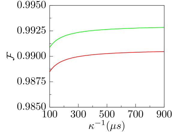
Figure 4: (Color online) Fidelity versus $\kappa^{-1}$. The green curve is based on the effective Hamitonian (4) and considering decoherence and the inter-cavity crosstalk; while the red curve is based on the full Hamiltonian $\widetilde{H}_{I}$ and considering decoherence and the inter-cavity crosstalk. From the red curve and the green curve, it can be seen that the fidelity for the gate performed in a realistic situation is slightly decreased by $\sim 0.25\%$, when compared to the case of the gate performed based on the effective Hamiltonian (4). This result implies that the approximations, which we made for obtaining the effective Hamiltonian (4), are reasonable.

For a transmon qutrit, the level spacing anharmonicity $100\sim 500$ MHz was reported in experiments s20 . As an example, consider $\omega_{eg}/2\pi=6.5$ GHz, $\omega_{fe}/2\pi=6.2$ GHz, $\omega_{c_{1}}/2\pi=7.0$ GHz, $\omega_{c_{2}}/2\pi=5.69$ GHz, and $\omega_{c_{3}}/2\pi=5.68$ GHz. Thus, $\left|\delta_{1}\right|/2\pi=0.5$ GHz, $\left|\delta_{2}\right|/2\pi=0.51$ GHz, $\left|\delta_{3}\right|/2\pi=0.52$ GHz, $\left|\widetilde{\delta}_{1}\right|/2\pi=0.8$ GHz, $\left|\widetilde{\delta}_{2}\right|/2\pi=0.81$ GHz, $\left|\widetilde{\delta}_{3}\right|/2\pi=0.82$ GHz, $\Delta_{12}/2\pi=0.01$ GHz, $\Delta_{13}/2\pi=0.02$ GHz, $\widetilde{\Delta}_{12}/2\pi=1.31$ GHz, $\widetilde{\Delta}_{23}/2\pi=0.01$ GHz, and $\widetilde{\Delta}_{13}/2\pi=1.32$ GHz.

Other parameters used in the numerical simulation are: (i) $\gamma_{eg}^{-1}=60$ $\mu$s, $\gamma_{fg}^{-1}=150$ $\mu$s s21 , $\gamma_{fe}^{-1}=30$ $\mu$s, $\gamma_{\phi e}^{-1}=\gamma_{\phi f}^{-1}=20$ $\mu$s, (ii) $g_{1}/2\pi=35$ MHz, (iii) $g_{kl}=0.01g_{\max}$ s22 , with $g_{\max}=\max\{g_{1},g_{2},g_{3}\}$, (iv) $\kappa_{1}=\kappa_{2}=\kappa_{3}=\kappa$, and (v) $\alpha=0.5$. According to Eq. (13), we have $g_{2}/2\pi\sim 50.5$ MHz and $g_{3}/2\pi\sim 72.1$ MHz. For a transmon qutrit [11], we have $\widetilde{g}_{1}\sim\sqrt{2}g_{1}\sim 2\pi\cdot 49.5$ MHz, $\widetilde{g}_{2}\sim g_{2}/\sqrt{2}\sim 2\pi\cdot 35.7$ MHz, and $\widetilde{g}_{3}\sim g_{3}/\sqrt{2}\sim 2\pi\cdot 41.6$ MHz. Here, we consider a rather conservative case for decoherence time of the transmon qutrit s6 ; s23 . In addition, the coupling constants here are readily available in experiments s24 .

By solving the master equation (15), we numerically calculate the fidelity versus $\kappa^{-1}$ as depicted in Fig. 4. The red curve is plotted based on the full Hamiltonian $\widetilde{H}_{I}$ and by considering the decoherence and the inter-cavity crosstalk. From the red curve one can see that when $\kappa^{-1}\geq 300$ $\mu$s, fidelity exceeds $0.9899$. The operation time is $\sim 0.41$ $\mu$s, much shorter than decoherence time of the qutrit used in the numerical calculation and the cavity decay times ($100~{}\mu$s - $900~{}\mu$s) considered in Fig. 4. Note that lifetime $\sim 1$ ms of microwave photons was experimentally demonstrated in a 3D microwave cavity s6 ; s25 . For the cavity frequencies given above and $\kappa^{-1}=300$ $\mu$s, the cavity quality factors are $Q_{1}\sim 1.31\times 10^{7}$ for cavity $1$, $Q_{2}\sim 1.07\times 10^{7}$ for cavity $2$, and $Q_{3}\sim 1.07\times 10^{7}$ for cavity $3,$ which are available because a high quality factor $Q=3.5\times 10^{7}$ of a 3D superconducting cavity has been demonstrated in experiments s25 . The analysis here implies that high-fidelity creation of a three-cat-state-qubit GHZ state is feasible with the present circuit QED technology.

Funding Information

This work was supported in part by the NKRDP of China (Grant No. 2016YFA0301802) and the National Natural Science Foundation of China under Grant Nos. [11074062, 11374083,11774076].

References

(1) N. Ofek, A. Petrenko, R. Heeres, P. Reinhold, Z. Leghtas, B.
Vlastakis, Y. Liu, L. Frunzio, S. M. Girvin, and L. Jiang, M. Mirrahimi, M. H. Devoret, and R. J. Schoelkopf,
Nature 536, 441 (2016).
(2) M. Mirrahimi, Z. Leghtas, V. V. Albert, S. Touzard, R. J.
Schoelkopf, L. Jiang, and M. H. Devoret, New J. Phys. 16, 045014
(2014).
(3) S. E. Nigg, Phys. Rev. A 89, 022340 (2014).
(4) C. P. Yang, Q. P. Su, S. B. Zheng, F. Nori, and S. Han, Phys.
Rev. A 95, 052341 (2017).
(5) R. W. Heeres, P. Reinhold, N. Ofek, L. Frunzio, L. Jiang, M. H.
Devoret, and R. J. Schoelkopf, arXiv:1608.02430, (2016).
(6) C. Wang, Y. Y. Gao, P. Reinhold, R. W. Heeres, N. Ofek, K.
Chou, C. Axline, M. Reagor, J. Blumoff, and K. M. Sliwa, L. Frunzio, S. M. Girvin,
L. Jiang, M. Mirrahimi, M. H. Devoret, and R. J. Schoelkopf,
Science 352, 1087 (2016).
(7) J. Clarke and F. K. Wilhelm, Nature 453, 1031 (2008).
(8) J. Q. You and F. Nori, Nature 474, 400 589 (2011).
(9) X. Gu, A. F. Kockum, A. Miranowicz, Y. X. Liu, and F. Nori,
Phys. Rep. 718-719, 1-102 (2017).
(10) M. Hillery, V. Buzek, and A. Berthiaume, Phys. Rev. A 59, 1829 (1999).
(11) S. Bose, V. Vedral, and P. L. Knight, Phys. Rev. A 57, 822(1998).
(12) J. J. Bollinger, W. M. Itano, D. J. Wineland, and D. J.
Heinzen, Phys. Rev. A 54, 4649 (1996).
(13) J. Koch, T. M. Yu, J. Gambetta, A. A. Houck, D. I. Schuster,
J. Majer, A. Blais, M. H. Devoret, S. M. Girvin, and R. J. Schoelkopf, Phys.
Rev. A 76, 042319 (2007).
(14) P. J. Leek, S. Filipp, P. Maurer, M. Baur, R. Bianchetti, J.
M. Fink, M. Goppl, L. Steffen, and A. Wallraff, Phys. Rev. B 79,
180511 (2009).
(15) M. Neeley, M. Ansmann, R. C. Bialczak, M. Hofheinz, N. Katz,
Erik Lucero, A. O’Connell, H. Wang, A. N. Cleland and J. M. Martinis, Nat.
Phys. 4, 523 (2008).
(16) M. Sandberg, C. M. Wilson, F. Persson, T. Bauch, G. Johansson,
V. Shumeiko, T. Duty, and P. Delsing, Appl. Phys. Lett. 92, 203501
(2008).
(17) Z. L. Wang, Y. P. Zhong, L. J. He, H. Wang, J. M. Martinis, A.
N. Cleland, and Q. W. Xie, Appl. Phys. Lett. 102, 163503 (2013).
(18) D. F. James and J. Jerke, Can. J. Phys. 85, 625
(2007).
(19) Qi-Ping Su, H. H. Zhu, L. Yu, Y. Zhang, S. J. Xiong, J. M.
Liu, and C. P. Yang, Phys. Rev. A 95, 022339 (2017).
(20) T. Niemczyk, F. Deppe, H. Huebl, E. P. Menzel, F. Hocke, M. J. Schwarz, J. J. Garcia-Ripoll,
D. Zueco, T. Hümmer, E. Solano, A. Marx and R. Gross,
Nat. Phys. 6, 772 (2010).
(21) For a transmon qutrit, the transition is much weaker than those of the and transitions. Thus, we have .
(22) S. J. Xiong, Z. Sun, J. M. Liu, T. Liu, and C. P. Yang, Optics
Letters 40, 2221 (2015).
(23) M. J. Peterer, S. J. Bader, X. Jin, F. Yan, A. Kamal, T. J.
Gudmundsen, P. J. Leek, T. P. Orlando, W. D. Oliver, and S. Gustavsson,
Phys. Rev. Lett. 114, 010501 (2015).
(24) A. Fedorov, L. Steffen, M. Baur, M. P. da Silva, and A.
Wallraff, Nature 481, 170 (2011).
(25) M. Reagor, W. Pfaff, C. Axline, R. W. Heeres, N. Ofek, K.
Sliwa, E. Holland, C. Wang, J. Blumoff, and K. Chou, M. J. Hatridge, L.Frunzio, M. H. Devoret, L. Jiang, and R. J. Schoelkopf,
Phys. Rev. B 94, 014506 (2016).