The Quantum Approximate Optimization Algorithm and the Sherrington-Kirkpatrick Model at Infinite Size

Edward Farhi Affiliation: Google Inc., Venice, CA 90291, USA Affiliation: Center for Theoretical Physics, Massachusetts Institute of Technology, Cambridge, MA 02139, USA    Jeffrey Goldstone Affiliation: Center for Theoretical Physics, Massachusetts Institute of Technology, Cambridge, MA 02139, USA    Sam Gutmann    Leo Zhou Affiliation: Google Inc., Venice, CA 90291, USA Affiliation: Department of Physics, Harvard University, Cambridge, MA 02138, USA
Abstract

The Quantum Approximate Optimization Algorithm (QAOA) is a general-purpose algorithm for combinatorial optimization problems whose performance can only improve with the number of layers pp. While QAOA holds promise as an algorithm that can be run on near-term quantum computers, its computational power has not been fully explored. In this work, we study the QAOA applied to the Sherrington-Kirkpatrick (SK) model, which can be understood as energy minimization of nn spins with all-to-all random signed couplings. There is a recent classical algorithm [1] that, assuming a widely believed conjecture, can efficiently find an approximate solution for a typical instance of the SK model to within (1ϵ)(1-\epsilon) times the ground state energy. We hope to match its performance with the QAOA.

Our main result is a novel technique that allows us to evaluate the typical-instance energy of the QAOA applied to the SK model. We produce a formula for the expected value of the energy, as a function of the 2p2p QAOA parameters, in the infinite size limit that can be evaluated on a computer with O(16p)O(16^{p}) complexity. We evaluate the formula up to p=12p=12, and find that the QAOA at p=11p=11 outperforms the standard semidefinite programming algorithm. Moreover, we show concentration: With probability tending to one as nn\to\infty, measurements of the QAOA will produce strings whose energies concentrate at our calculated value. As an algorithm running on a quantum computer, there is no need to search for optimal parameters on an instance-by-instance basis since we can determine them in advance. What we have here is a new framework for analyzing the QAOA, and our techniques can be of broad interest for evaluating its performance on more general problems where classical algorithms may fail.

1 Introduction

The Quantum Approximate Optimization Algorithm [2], QAOA, consists of a shallow depth quantum circuit with pp layers and 2p2p parameters. It is designed to find approximate solutions to combinatorial search problems, and like simulated annealing can be applied to almost any problem. As pp increases, performance can only improve. Even at p=1p=1, worst case performance guarantees have been established [2, 3]. These beat random guessing but not the best classical algorithms. Aside from worst case we can ask how the QAOA performs on typical instances where the problem instances are drawn from a specified distribution. For example, for the combinatorial search problem E3LIN2, a worst case performance guarantee was established but the typical performance is better [3]. For similar results on other problems see Lin and Zhu [4].

A key insight for typical instances, drawn from a specified distribution, is the landscape independence [5] of the expected value of the cost function in the parameter dependent quantum state: Given an instance of a combinatorial search problem and a set of control parameters, the QAOA quantum state depends both on the instance and the parameters. However for large systems, the expected value of the cost function in the quantum state depends on the parameters but not the instance, up to finite size effects. This means that for each value of pp, the optimal parameters are the same for typical instances coming from the distribution. Although the optimal parameters may be known, one still needs to run the quantum computer for each instance to find a string which achieves the optimal cost function value attainable at a given pp.

In this paper, we introduce a novel technique for evaluating the typical-instance energy of the QAOA applied to a combinatorial search problem for arbitrary fixed pp as the problem size goes to infinity. We apply the QAOA to the Sherrington-Kirkpatrick model. This model can be seen as a combinatorial search problem on a complete graph with random couplings. For typical instances, the value of the lowest energy is known [6, 7, 8, 9]. Assuming a widely believed conjecture about the model, there is also a recent polynomial-time classical algorithm for finding a string whose energy is between (1ϵ)(1-\epsilon) times the lowest energy and the lowest energy with high probability [1]. What we have accomplished is a method for calculating, in advance, what energy the QAOA will produce for given parameters at any fixed pp in the infinite size limit. We also show concentration, i.e., with probability tending to one as nn\to\infty, measurements of the QAOA will produce strings whose energies concentrate at our calculated value. This concentration result implies landscape independence for this model, similar to what was found for bounded degree graphs in [5]. This means that optimal parameters found for one large instance will also be good for other large instances. The complexity of our calculation scales as O(16p)O(16^{p}), and the answer is evaluated on a computer. Without much trouble, we have found optimal parameters up to p=8p=8, and further evaluated the performance up to p=12p=12 at extrapolated parameters. Notably, our results show that the QAOA surpasses the standard semidefinite programming algorithm at p=11p=11.

The paper is organized as follows. We first review the QAOA (Section 2) and the Sherrington-Kirkpatrick model (Section 3). The results of the paper are summarized in Section 4, where we produce a formula to calculate the typical-instance energy achieved by the QAOA for any pp with any given parameters, and show that the measured energy concentrates at the calculated value. We also evaluate the formula up to p=12p=12. In Section 5, we demonstrate how to calculate the typical-instance energy for the QAOA at p=1p=1 for any finite problem size. In Section 6, we prove the formula for general pp in the infinite size limit. We provide further discussion in Section 7.

2 The Quantum Approximate Optimization Algorithm (QAOA)

We start by reviewing the Quantum Approximate Optimization Algorithm (QAOA). Given a classical cost function C(𝒛)C({\boldsymbol{z}}) defined on nn-bit strings 𝒛=(z1,z2,,zn){+1,1}n{\boldsymbol{z}}=(z_{1},z_{2},\ldots,z_{n})\in\{+1,-1\}^{n}, the QAOA is a quantum algorithm that aims to find a string 𝒛{\boldsymbol{z}} such that C(𝒛)C({\boldsymbol{z}}) is close to its absolute minimum. The cost function CC can be written as an operator that is diagonal in the computational basis, defined as

C|𝒛=C(𝒛)|𝒛.C\ket{{\boldsymbol{z}}}=C({\boldsymbol{z}})\ket{{\boldsymbol{z}}}. (1)

We introduce a unitary operator that depends on CC and a parameter γ\gamma

U(C,γ)=eiγC.U(C,\gamma)=e^{-i\gamma C}. (2)

Additionally, we introduce the operator

B=j=1nXj,B=\sum_{j=1}^{n}X_{j}, (3)

where XjX_{j} is the Pauli XX operator acting on qubit jj, and an associated unitary operator that depends on a parameter β\beta

U(B,β)=eiβB=j=1neiβXj.U(B,\beta)=e^{-i\beta B}=\prod_{j=1}^{n}e^{-i\beta X_{j}}. (4)

In the QAOA circuit, we initialize the system of qubits in the state

|s=|+n=12n𝒛|𝒛,\ket{s}=\ket{+}^{\otimes n}=\frac{1}{\sqrt{2^{n}}}\sum_{{\boldsymbol{z}}}\ket{{\boldsymbol{z}}}, (5)

and alternately apply pp layers of U(C,γ)U(C,\gamma) and U(B,β)U(B,\beta). Let 𝜸=γ1,γ2,,γp\boldsymbol{\gamma}=\gamma_{1},\gamma_{2},\ldots,\gamma_{p} and 𝜷=β1,β2,,βp\boldsymbol{\beta}=\beta_{1},\beta_{2},\ldots,\beta_{p}; then the QAOA circuit prepares the following state

|𝜸,𝜷=U(B,βp)U(C,γp)U(B,β1)U(C,γ1)|s.\ket{\boldsymbol{\gamma},\boldsymbol{\beta}}=U(B,\beta_{p})U(C,\gamma_{p})\cdots U(B,\beta_{1})U(C,\gamma_{1})\ket{s}. (6)

For a given cost function CC, the associated QAOA objective function is

𝜸,𝜷|C|𝜸,𝜷.\braket{\boldsymbol{\gamma},\boldsymbol{\beta}|C|\boldsymbol{\gamma},\boldsymbol{\beta}}. (7)

By measuring the quantum state |𝜸,𝜷\ket{\boldsymbol{\gamma},\boldsymbol{\beta}} in the computational basis, one will find a bit string 𝒛{\boldsymbol{z}} such that C(𝒛)C({\boldsymbol{z}}) is near (7) or better. Different strategies have been developed to find optimal (𝜸,𝜷)(\boldsymbol{\gamma},\boldsymbol{\beta}) for any given instance [5, 10, 11]. In this paper, however, we will show how to find, in advance, the optimal parameters of the QAOA at fixed pp for typical instances of the Sherrington-Kirkpatrick model.

3 The Sherrington-Kirkpatrick (SK) model

In this paper, we apply the QAOA to instances of the Sherrington-Kirkpatrick model, which is central to many important results in the theory of spin glass and disordered systems (see [7] for a review). This model describes a classical spin system with all-to-all couplings between the nn spins. The classical cost function is

C(𝒛)=1nj<kJjkzjzk.C({\boldsymbol{z}})=\frac{1}{\sqrt{n}}\sum_{j<k}J_{jk}z_{j}z_{k}. (8)

Each instance is specified by the JjkJ_{jk}’s which are independently chosen from a distribution with mean 0 and variance 1. For example they could be +1+1 or 1-1 each with probability 1/2, or drawn from the standard normal distribution. In this paper, we assume JjkJ_{jk} comes from a symmetrical distribution (i.e., JjkJ_{jk} and Jjk-J_{jk} have the same distribution), although we believe generalization to any subgaussian distribution is not too difficult. As nn goes to infinity, the classical results as well as our quantum results are independent of which distribution the JjkJ_{jk}’s come from. In a celebrated result, Parisi calculated the lowest energy of (8) for typical instances as nn goes to infinity. The first step is to consider the partition function

𝒛exp(C(𝒛)/T)\sum_{{\boldsymbol{z}}}\exp(-C({\boldsymbol{z}})/T) (9)

which is dominated by the low energy configurations for low temperature TT. Averaging this quantity over the JjkJ_{jk}’s is easy but gives the wrong description at low temperature. One needs to first take the log and then average:

Tn𝔼J[log(𝐳exp(C(𝐳)/T))].\frac{T}{n}\EV_{J}\Big[\log\Big(\sum_{{\boldsymbol{z}}}\exp(-C({\boldsymbol{z}})/T)\Big)\Big]. (10)

In the limit of nn\to\infty, this quantity has been proven to exist, although evaluating this quantity is extremely challenging. Using the method of replica symmetry breaking, Parisi [6] provides a formula (for proof, see [7]) that, when numerically evaluated [8, 9, 1], shows for typical instances,

limnmin𝒛C(𝒛)n=0.763166.\lim_{n\to\infty}\min_{{\boldsymbol{z}}}\frac{C({\boldsymbol{z}})}{n}=-0.763166\ldots. (11)

We note that this model has a phase transition at T=1T=1, and that at this temperature, C/nC/n is 0.5-0.5 for typical instances.

The result just given tells us what the lowest energy of the SK model is, but it does not tell us how to find the associated configuration. How hard is this? Simulated annealing does rather well in getting a string whose energy is close to the minimum. For example running simulated annealing starting at a temperature above the phase transition, say T=1.3T=1.3, and bringing it down to near T=0T=0 in 10 million steps on a 10000 bit instance achieves 0.754-0.754. It is not believed that simulated annealing can go all the way to the lowest energy configuration [12]. We can also ask how zero-temperature simulated annealing performs. Here the update rule is flip a spin if it lowers the energy, and don’t flip if it does not. This algorithm comes down to around 0.71-0.71.

Another natural approach to solve this problem is a convex relaxation method such as semidefinite programming. The simplest such method is called spectral relaxation, where the solution is obtained by taking the lowest eigenvector of the n×nn\times n matrix 𝑱\boldsymbol{J} (whose elements are given by JjkJ_{jk}), and rounding each entry to ±1\pm 1 based on its sign. This yields C/n=2/π+o(1)0.6366C/n=-2/\pi+o(1)\approx-0.6366 [13], where o(1)o(1) is a number that vanishes as nn\to\infty. The standard semidefinite programming algorithm with “sign rounding” yields the same result [14, 15].

Recently, assuming a widely believed yet unproven conjecture that the SK model has “full replica symmetry breaking,” Montanari gave an algorithm [1] that finds a string whose energy is below (1ϵ)(1-\epsilon) times the lowest energy for typical instances. The run time of this algorithm is c(ϵ)n2c(\epsilon)n^{2}, and the function c(ϵ)c(\epsilon) is an inverse polynomial of ϵ\epsilon.

4 Summary of Results

We analyze how the QAOA performs on the SK model by evaluating

𝔼J[𝜸,𝜷|C/n|𝜸,𝜷]and𝔼J[𝜸,𝜷|(C/n)2|𝜸,𝜷]\EV_{J}\left[\braket{\boldsymbol{\gamma},\boldsymbol{\beta}|C/n|\boldsymbol{\gamma},\boldsymbol{\beta}}\right]\quad\text{and}\quad\EV_{J}\left[\braket{\boldsymbol{\gamma},\boldsymbol{\beta}|(C/n)^{2}|\boldsymbol{\gamma},\boldsymbol{\beta}}\right] (12)

in the infinite size nn\to\infty limit. Note that both CC and |𝜸,𝜷\ket{\boldsymbol{\gamma},\boldsymbol{\beta}} depend on JJ. Our main result, which will be proved in Section 6, is the following:

Theorem.

For any pp and any parameters (𝛄,𝛃)(\boldsymbol{\gamma},\boldsymbol{\beta}), we have

limn𝔼J[𝜸,𝜷|C/n|𝜸,𝜷]\displaystyle\lim_{n\to\infty}\EV_{J}\left[\braket{\boldsymbol{\gamma},\boldsymbol{\beta}|C/n|\boldsymbol{\gamma},\boldsymbol{\beta}}\right] =Vp(𝜸,𝜷),\displaystyle=V_{p}(\boldsymbol{\gamma},\boldsymbol{\beta}), (13)

where Vp(𝛄,𝛃)V_{p}(\boldsymbol{\gamma},\boldsymbol{\beta}) has an explicit formula that we give below in Eq. (33). Furthermore, we have

limn𝔼J[𝜸,𝜷|(C/n)2|𝜸,𝜷]=[Vp(𝜸,𝜷)]2.\displaystyle\lim_{n\to\infty}\EV_{J}\left[\braket{\boldsymbol{\gamma},\boldsymbol{\beta}|(C/n)^{2}|\boldsymbol{\gamma},\boldsymbol{\beta}}\right]=[V_{p}(\boldsymbol{\gamma},\boldsymbol{\beta})]^{2}. (14)

Note the above theorem easily implies the following corollary which shows that the QAOA exhibits strong concentration properties:

Corollary (Concentration).

At any fixed pp and for any parameters (𝛄,𝛃)(\boldsymbol{\gamma},\boldsymbol{\beta}), the energy produced by the QAOA on almost every instance of the SK model concentrates at Vp(𝛄,𝛃)V_{p}(\boldsymbol{\gamma},\boldsymbol{\beta}) in the limit as nn\to\infty. Specifically, we have concentration over instances, i.e., for every ϵ>0\epsilon>0,

J(|𝜸,𝜷|C/n|𝜸,𝜷Vp(𝜸,𝜷)|>ϵ)0asn.\displaystyle\mathbb{P}_{J}\left(\Big|\braket{\boldsymbol{\gamma},\boldsymbol{\beta}|C/n|\boldsymbol{\gamma},\boldsymbol{\beta}}-V_{p}(\boldsymbol{\gamma},\boldsymbol{\beta})\Big|>\epsilon\right)\to 0\qquad\text{as}\qquad n\to\infty. (15)

We also have concentration over measurements, i.e., for every ϵ>0\epsilon>0,

𝔼J[𝐳 measured from |𝜸,𝜷(|C(𝐳)/n𝜸,𝜷|C/n|𝜸,𝜷|>ϵ)]0asn.\displaystyle\EV_{J}\Big[\mathbb{P}_{{\boldsymbol{z}}\textnormal{ measured from }\ket{\boldsymbol{\gamma},\boldsymbol{\beta}}}\left(\Big|C({\boldsymbol{z}})/n-\braket{\boldsymbol{\gamma},\boldsymbol{\beta}|C/n|\boldsymbol{\gamma},\boldsymbol{\beta}}\Big|>\epsilon\right)\Big]\to 0\qquad\text{as}\qquad n\to\infty. (16)
Proof of Corollary.

Combining (13) and (14), we have

limn(𝔼J[𝜸,𝜷|(C/n)2|𝜸,𝜷]𝔼J2[𝜸,𝜷|C/n|𝜸,𝜷])=0.\displaystyle\lim_{n\to\infty}\left(\EV_{J}[\braket{\boldsymbol{\gamma},\boldsymbol{\beta}|(C/n)^{2}|\boldsymbol{\gamma},\boldsymbol{\beta}}]-\EV_{J}^{2}[\braket{\boldsymbol{\gamma},\boldsymbol{\beta}|C/n|\boldsymbol{\gamma},\boldsymbol{\beta}}]\right)=0. (17)

Since for any operator OO,

O2O2,\displaystyle\braket{O}^{2}\leq\braket{O^{2}}, (18)

we have

𝔼J[𝜸,𝜷|C/n|𝜸,𝜷2]𝔼J2[𝜸,𝜷|C/n|𝜸,𝜷]\displaystyle\EV_{J}[\braket{\boldsymbol{\gamma},\boldsymbol{\beta}|C/n|\boldsymbol{\gamma},\boldsymbol{\beta}}^{2}]-\EV_{J}^{2}[\braket{\boldsymbol{\gamma},\boldsymbol{\beta}|C/n|\boldsymbol{\gamma},\boldsymbol{\beta}}] 𝔼J[𝜸,𝜷|(C/n)2|𝜸,𝜷]𝔼J2[𝜸,𝜷|C/n|𝜸,𝜷].\displaystyle\leq\EV_{J}[\braket{\boldsymbol{\gamma},\boldsymbol{\beta}|(C/n)^{2}|\boldsymbol{\gamma},\boldsymbol{\beta}}]-\EV_{J}^{2}[\braket{\boldsymbol{\gamma},\boldsymbol{\beta}|C/n|\boldsymbol{\gamma},\boldsymbol{\beta}}]. (19)

Note that as nn\to\infty, the right hand side vanishes, which implies

limn(𝔼J[𝜸,𝜷|C/n|𝜸,𝜷2]𝔼J2[𝜸,𝜷|C/n|𝜸,𝜷])=0.\displaystyle\lim_{n\to\infty}\left(\EV_{J}[\braket{\boldsymbol{\gamma},\boldsymbol{\beta}|C/n|\boldsymbol{\gamma},\boldsymbol{\beta}}^{2}]-\EV_{J}^{2}[\braket{\boldsymbol{\gamma},\boldsymbol{\beta}|C/n|\boldsymbol{\gamma},\boldsymbol{\beta}}]\right)=0. (20)

By Chebyshev’s inequality, this implies (15), which proves landscape independence [5] for the SK model.

To show concentration over measurements for fixed JJ, we subtract (20) from (17) to give us

𝔼J[𝜸,𝜷|(C/n)2|𝜸,𝜷𝜸,𝜷|C/n|𝜸,𝜷2]\displaystyle\EV_{J}\Big[\braket{\boldsymbol{\gamma},\boldsymbol{\beta}|(C/n)^{2}|\boldsymbol{\gamma},\boldsymbol{\beta}}-\braket{\boldsymbol{\gamma},\boldsymbol{\beta}|C/n|\boldsymbol{\gamma},\boldsymbol{\beta}}^{2}\Big] 0asn.\displaystyle\longrightarrow 0\qquad\text{as}\qquad n\to\infty. (21)

By (18) for any JJ

𝜸,𝜷|(C/n)2|𝜸,𝜷𝜸,𝜷|C/n|𝜸,𝜷20,\braket{\boldsymbol{\gamma},\boldsymbol{\beta}|(C/n)^{2}|\boldsymbol{\gamma},\boldsymbol{\beta}}-\braket{\boldsymbol{\gamma},\boldsymbol{\beta}|C/n|\boldsymbol{\gamma},\boldsymbol{\beta}}^{2}\geq 0, (22)

Then (21) shows that this variance vanishes typically as nn\to\infty. This implies (16) by Chebyshev’s inequality. ∎

This corollary means that as nn\to\infty, for typical instances of the SK model, upon applying the QAOA and measuring in the computational basis, we will obtain a string 𝒛{\boldsymbol{z}} that has energy C(𝒛)/nC({\boldsymbol{z}})/n close to 𝜸,𝜷|C/n|𝜸,𝜷\braket{\boldsymbol{\gamma},\boldsymbol{\beta}|C/n|\boldsymbol{\gamma},\boldsymbol{\beta}}, which is itself close to Vp(𝜸,𝜷)V_{p}(\boldsymbol{\gamma},\boldsymbol{\beta}).

Formula for Vp(𝜸,𝜷)V_{p}(\boldsymbol{\gamma},\boldsymbol{\beta})

— We now provide instructions on how to evaluate Vp(𝜸,𝜷)V_{p}(\boldsymbol{\gamma},\boldsymbol{\beta}). Start by defining

A={(a1,,ap,ap,,a1):a±j=+1,1}A=\{(a_{1},\ldots,a_{p},a_{-p},\ldots,a_{-1}):a_{\pm j}=+1,-1\} (23)

as the set of all configurations. We partition into A=A1ApAp+1A=A_{1}\cup\cdots\cup A_{p}\cup A_{p+1}, where

A={𝒂:ak=ak for p+1<kp, and ap+1=ap+1}for1p,A_{\ell}=\{{\boldsymbol{a}}:a_{-k}=a_{k}\text{ for }p-\ell+1<k\leq p,\text{ and }a_{-p+\ell-1}=-a_{p-\ell+1}\}\quad\text{for}\quad 1\leq\ell\leq p, (24)

and

Ap+1={𝒂:ak=ak for 1kp}.A_{p+1}=\{{\boldsymbol{a}}:a_{-k}=a_{k}\text{ for }1\leq k\leq p\}\,. (25)

We define a * operation which transforms configuration 𝒂{\boldsymbol{a}} into 𝒂{\boldsymbol{a}}^{*} given by

ar=arar+1apandar=arar1apfor 1rp.a^{*}_{r}=a_{r}a_{r+1}\cdots a_{p}\qquad\text{and}\qquad a^{*}_{-r}=a_{-r}a_{-r-1}\cdots a_{-p}\quad\text{for }1\leq r\leq p\,. (26)

For any 𝒂,𝒃A{\boldsymbol{a}},{\boldsymbol{b}}\in A, let

Q𝒂=j=1p(cosβj)1+(aj+aj)/2(sinβj)1(aj+aj)/2(i)(ajaj)/2,\displaystyle Q_{\boldsymbol{a}}=\prod_{j=1}^{p}(\cos\beta_{j})^{1+(a_{j}+a_{-j})/2}(\sin\beta_{j})^{1-(a_{j}+a_{-j})/2}(i)^{(a_{-j}-a_{j})/2}, (27)
Φ𝒂=r=1pγr(arar),andX𝒃=Q𝒃exp(12𝒂Ap+1Q𝒂Φ𝒂𝒃2).\displaystyle\Phi_{\boldsymbol{a}}=\sum_{r=1}^{p}\gamma_{r}(a^{*}_{r}-a^{*}_{-r}),\qquad\text{and}\qquad X_{\boldsymbol{b}}=Q_{\boldsymbol{b}}\exp\Big({-}\frac{1}{2}{\sum_{{\boldsymbol{a}}\in A_{p+1}}Q_{\boldsymbol{a}}\Phi^{2}_{{\boldsymbol{a}}{\boldsymbol{b}}}}\Big). (28)

Furthermore, for any 𝒂,𝒃AAp+1{\boldsymbol{a}},{\boldsymbol{b}}\in A\setminus A_{p+1}, let

Δ𝒂,𝒃=12(Φ𝒂¯𝒃2Φ𝒂𝒃2)\displaystyle\Delta_{{\boldsymbol{a}},{\boldsymbol{b}}}=\frac{1}{2}(\Phi^{2}_{\bar{\boldsymbol{a}}{\boldsymbol{b}}}-\Phi^{2}_{{\boldsymbol{a}}{\boldsymbol{b}}}) (29)

where the 𝒂¯\bar{{\boldsymbol{a}}} operation takes configuration 𝒂A{\boldsymbol{a}}\in A_{\ell} to 𝒂¯A\bar{\boldsymbol{a}}\in A_{\ell} for 1p1\leq\ell\leq p via

a¯±r={a±r,rp+1a±rr=p+1.\displaystyle\bar{a}_{\pm r}=\begin{cases}a_{\pm r},&r\neq p-\ell+1\\ -a_{\pm r}&r=p-\ell+1\end{cases}\,. (30)

We then bipartition B=AAp+1B=A\setminus A_{p+1} into two sets DDcD\cup D^{c}, such that if 𝒃D{\boldsymbol{b}}\in D then 𝒃¯Dc\bar{\boldsymbol{b}}\in D^{c}. Note |D|=|B|/2=(22p2p)/2|D|=|B|/2=(2^{2p}-2^{p})/2. For concreteness, we can use the convention where all configurations of DD are chosen so that their first pp elements have even parity. Furthermore, for each element 𝒃D{\boldsymbol{b}}\in D we assign an index j(𝒃){1,2,,|D|}j({\boldsymbol{b}})\in\{1,2,\ldots,|D|\}, such that if j(𝒃)j(𝒃)j({\boldsymbol{b}})\leq j({\boldsymbol{b}}^{\prime}) then Φ𝒃¯𝒃2=Φ𝒃𝒃2\Phi_{\bar{\boldsymbol{b}}{\boldsymbol{b}}^{\prime}}^{2}=\Phi^{2}_{{\boldsymbol{b}}{\boldsymbol{b}}^{\prime}} (and we say “𝒃{\boldsymbol{b}} plays well with 𝒃{\boldsymbol{b}}^{\prime}”). This index can be efficiently assigned since 𝒃A{\boldsymbol{b}}\in A_{\ell} plays well with 𝒃A{\boldsymbol{b}}^{\prime}\in A_{\ell^{\prime}} if \ell\leq\ell^{\prime} (see Lemma 1 in Section 6.1). With this index assignment, we have Δk,j=0\Delta_{k,j}=0 for kjk\leq j.

Next, for every element of 𝒖D{\boldsymbol{u}}\in D we assign a value W𝒖W_{\boldsymbol{u}} which can be iteratively obtained as follows: Start with W|D|=X|D|W_{|D|}=X_{|D|}, and for j=|D|1,,2,1j=|D|-1,\ldots,2,1 compute

Wj=Xjexp(k=j+1|D|WkΔk,j).W_{j}=X_{j}\exp\left({\textstyle\sum_{k=j+1}^{|D|}W_{k}\Delta_{k,j}}\right). (31)

Then for other elements 𝒖D{\boldsymbol{u}}\not\in D we assign

W𝒖=Q𝒖when𝒖Ap+1, and W𝒖¯=W𝒖when𝒖¯Dc.W_{\boldsymbol{u}}=Q_{\boldsymbol{u}}\quad\text{when}\quad{\boldsymbol{u}}\in A_{p+1},\qquad\text{ and }\qquad W_{\bar{\boldsymbol{u}}}=-W_{\boldsymbol{u}}\quad\text{when}\quad\bar{\boldsymbol{u}}\in D^{c}. (32)

Finally, Vp(𝜸,𝜷)V_{p}(\boldsymbol{\gamma},\boldsymbol{\beta}) is obtained from all the W𝒖W_{\boldsymbol{u}}’s via the following formula:

Vp(𝜸,𝜷)=i2r=1pγr[𝒖A(ur+ur)W𝒖][𝒗A(vrvr)W𝒗].V_{p}(\boldsymbol{\gamma},\boldsymbol{\beta})=\frac{i}{2}\sum_{r=1}^{p}\gamma_{r}\left[\sum_{{\boldsymbol{u}}\in A}(u^{*}_{r}+u^{*}_{-r})W_{\boldsymbol{u}}\right]\left[\sum_{{\boldsymbol{v}}\in A}(v^{*}_{r}-v^{*}_{-r})W_{\boldsymbol{v}}\right]\,. (33)

The memory complexity of the above computation is at most O(4p){O}(4^{p}) for storing the vector of W𝒖W_{\boldsymbol{u}}’s which has dimension |D|=(4p2p)/2|D|=(4^{p}-2^{p})/2. Computing all the W𝒖W_{{\boldsymbol{u}}}’s requires evaluating (31) |D||D| times, each involving a sum of at most |D||D| terms. Hence, we only need at most O(|D|2)=O(16p)O(|D|^{2})=O(16^{p}) time to compute the W𝒖W_{\boldsymbol{u}}’s. Once we have an array of W𝒖W_{\boldsymbol{u}} in memory, computing VpV_{p} takes at most O(p 4p)O(p\,4^{p}) extra time as we simply add up W𝒖W_{\boldsymbol{u}} for some pp pairs of subsets of AA and multiply the results. The time complexity for computing VpV_{p} is thus at most O(16p)O(16^{p}).

Numerical evaluation and optimization

— Here, we give our results optimizing

Vp(𝜸,𝜷)=limn𝔼[𝜸,𝜷|C/n|𝜸,𝜷],V_{p}(\boldsymbol{\gamma},\boldsymbol{\beta})=\lim_{n\to\infty}\EV[\braket{\boldsymbol{\gamma},\boldsymbol{\beta}|C/n|\boldsymbol{\gamma},\boldsymbol{\beta}}], (34)

with respect to the QAOA parameters 𝜸\boldsymbol{\gamma} and 𝜷\boldsymbol{\beta}. For a given pp, we denote the optimal value as

V¯p=min𝜸,𝜷Vp(𝜸,𝜷).\displaystyle\bar{V}_{p}=\min_{\boldsymbol{\gamma},\boldsymbol{\beta}}V_{p}(\boldsymbol{\gamma},\boldsymbol{\beta}). (35)

Using a laptop to calculate Vp(𝜸,𝜷)V_{p}(\boldsymbol{\gamma},\boldsymbol{\beta}) to floating point precision, and applying a heuristic for optimizing QAOA parameters [10], we are able to find optimal parameters up to p=8p=8. Furthermore, by performing the computation using a GPU on the Harvard FASRC Cannon cluster, we are able to calculate Vp(𝜸,𝜷)V_{p}(\boldsymbol{\gamma},\boldsymbol{\beta}) up to p=12p=12.

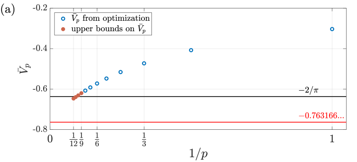
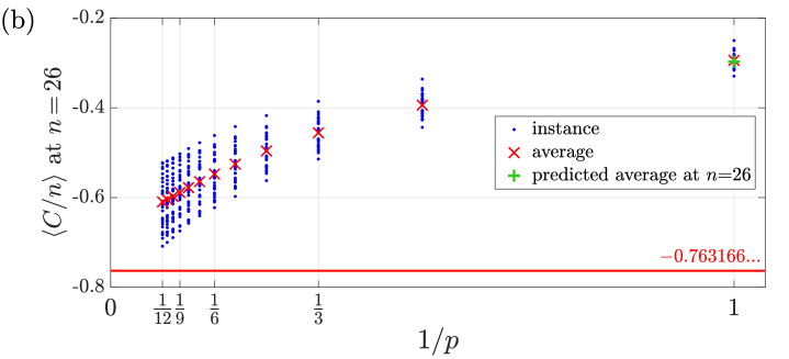
In Figure 1(a), we plot the values of the energy in the infinite size limit, Vp(𝜸,𝜷)V_{p}(\boldsymbol{\gamma},\boldsymbol{\beta}), at the parameters we have found. The values we have found for 9p129\leq p\leq 12 are not optimized but simply evaluated at some parameters extrapolated from those at lower pp. These values serve as upper bounds on the value of V¯p\bar{V}_{p}, since we are not always certain that the parameters we found are the best possible. It is shown to decrease steadily as pp increases, but it is unclear where or how fast it will asymptote. Nevertheless, the results show that the QAOA surpasses the standard semi-definite programming algorithm at p=11p=11, where V¯110.6393<2/π\bar{V}_{11}\leq-0.6393<-2/\pi. The known minimum energy of 0.763166-0.763166... from the Parisi ansatz as in (11) is shown as a red line. To confirm that our infinite size limit calculation gives reasonable predictions in the finite size case, we simulate the QAOA on 30 randomly tossed instances of the SK model with n=26n=26 spins and JjkJ_{jk} drawn from the standard normal distribution. In Figure 1(b), we plot the expectation value of the energy C/n\braket{C/n} for these instances, at the same optimized QAOA parameters used for the infinite size limit. It appears to give good agreement with the values in Figure 1(a), up to O(1/n)O(1/\sqrt{n}) finite size effects.

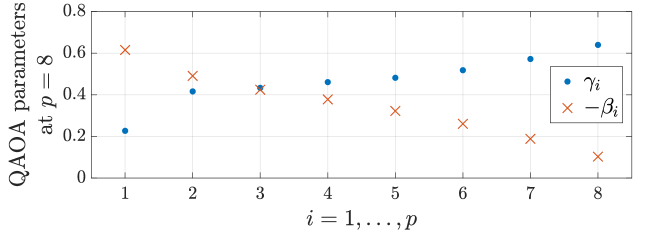
We have found that the optimal QAOA parameters for the SK model in the infinite size limit appear to have a pattern, similar to what was found in [10, 11]. As an example, we plot the optimal parameters for p=8p=8 in Figure 2. The full list of parameters and V¯p\bar{V}_{p} we found for 1p81\leq p\leq 8 are also given in Table 1. As we progress through the QAOA circuit, the optimal parameter γi\gamma_{i} appears to increase monotonically, and the parameter βi-\beta_{i} appears to decrease monotonically. We have exploited this pattern to obtain good guesses of parameters for 9p129\leq p\leq 12, which are listed in Table 2.

Figure 1: (a) Our results for V¯p=min𝜸,𝜷Vp(𝜸,𝜷)\bar{V}_{p}=\min_{\boldsymbol{\gamma},\boldsymbol{\beta}}V_{p}(\boldsymbol{\gamma},\boldsymbol{\beta}) as a function of pp. The values for p8p\leq 8 are based on optimizing Vp(𝜸,𝜷)=limn𝔼J[C/n]V_{p}(\boldsymbol{\gamma},\boldsymbol{\beta})=\lim_{n\to\infty}\EV_{J}\left[\braket{C/n}\right]. The values for 9p129\leq p\leq 12 are from evaluating Vp(𝜸,𝜷)V_{p}(\boldsymbol{\gamma},\boldsymbol{\beta}) at some parameters extrapolated from those at lower pp but not further optimized. Note at p=11p=11, QAOA is able to surpass 2/π0.6366-2/\pi\approx 0.6366, which is the performance of the standard semidefinite programming algorithm [1, 15]. The full set of values of VpV_{p} and the parameters are given in Table 1 and 2. (b) The expectation value of C/nC/n for 30 randomly tossed instances of 26-spin Sherrington-Kirkpatrick model with JjkJ_{jk} drawn from the standard normal distribution. The spread in values over the instances is a finite nn effect, since our concentration results show that the variance over instances goes to 0 as nn\to\infty. The average values over instances show good agreement with those above in (a). The pp = 1 predicted average at n=26n=26 from (62), which evaluates to 0.29726-0.29726, is also plotted.
Figure 2: The optimal parameters found for p=8p=8. We believe these to be globally optimal, based on the fact they appear repeatedly as the best local minimum when optimizing from 10410^{4} starting points uniformly randomly drawn from the range γi[2,2]\gamma_{i}\in[-2,2] and βi[π/4,π/4]\beta_{i}\in[-\pi/4,\pi/4].
pp V¯p\bar{V}_{p} optimized 𝜸\boldsymbol{\gamma} optimized 𝜷-\boldsymbol{\beta}
1 1/4e-1/\sqrt{4e}\approx 1/2 π/8\pi/8
0.3033-0.3033
2 0.4075-0.4075 0.3817, 0.6655 0.4960, 0.2690
3 0.4726-0.4726 0.3297, 0.5688, 0.6406 0.5500, 0.3675, 0.2109
4 0.5157-0.5157 0.2949, 0.5144, 0.5586, 0.6429 0.5710, 0.4176, 0.3028, 0.1729
5 0.5476-0.5476 0.2705, 0.4803, 0.5074 0.5899, 0.4492, 0.3559
0.5646, 0.6397 0.2643, 0.1486
6 0.5721-0.5721 0.2528, 0.4531, 0.4750 0.6004, 0.4670, 0.3880
0.5146, 0.5650, 0.6392 0.3176, 0.2325, 0.1291
0.2383, 0.4327, 0.4516, 0.6085, 0.4810, 0.4090,
7 0.5915-0.5915 0.4830, 0.5147, 0.3535, 0.2857,
0.5686, 0.6393 0.2080, 0.1146
0.2268, 0.4163, 0.4333, 0.6152, 0.4906, 0.4244,
8 0.6073-0.6073 0.4608, 0.4816, 0.5180, 0.3779, 0.3223, 0.2606,
0.5719, 0.6396 0.1884, 0.1030
Table 1: Our calculated values of V¯p=minlimn𝜸,𝜷𝔼[C/n]\bar{V}_{p}=\min_{\boldsymbol{\gamma},\boldsymbol{\beta}}\lim_{n\to\infty}\EV[\braket{C/n}] and optimized QAOA parameters (𝜸,𝜷)(\boldsymbol{\gamma},\boldsymbol{\beta}). These parameters, presented in the order of γ1,γ2,\gamma_{1},\gamma_{2},\ldots, etc., are optimized using heuristics from [10]. They are confirmed to be globally optimal by running optimization from 10410^{4} random starts and seeing the same values repeat.
pp Vp(𝜸,𝜷)V_{p}(\boldsymbol{\gamma},\boldsymbol{\beta}) 𝜸\boldsymbol{\gamma} 𝜷-\boldsymbol{\beta}
0.2166, 0.4051, 0.4208, 0.6226, 0.4994, 0.4410,
9 0.6199-0.6199 0.4455, 0.4641, 0.4944, 0.3888, 0.3527, 0.3031,
0.5309, 0.5801, 0.6396 0.2462, 0.1769, 0.0951
0.2081, 0.3938, 0.4087, 0.4315, 0.6275, 0.5059, 0.4454, 0.4089,
10 0.6308-0.6308 0.4473, 0.4742, 0.5015, 0.3676, 0.3344, 0.2866,
0.5385, 0.5850, 0.6396 0.2321, 0.1652, 0.0878
0.2007, 0.3840, 0.3983, 0.4197, 0.6317, 0.5111, 0.4525, 0.4192,
11 0.6393-0.6393 0.4336, 0.4583, 0.4811, 0.5096, 0.3824, 0.3444, 0.3197, 0.2730,
0.5458, 0.5895, 0.6396 0.2203, 0.1553, 0.0815
0.1941, 0.3753, 0.3892, 0.4096, 0.6353, 0.5155, 0.4583, 0.4274,
12 0.6466-0.6466 0.4221, 0.4452, 0.4654, 0.4889, 0.3940, 0.3600, 0.3305, 0.3076,
0.5175, 0.5524, 0.5934, 0.6396 0.2615, 0.2102, 0.1468, 0.0762
Table 2: The best known values (prior to Ref. [17]) of Vp=limn𝔼[C/n]V_{p}=\lim_{n\to\infty}\EV[\braket{C/n}] for 9p129\leq p\leq 12, and the corresponding QAOA parameters (𝜸,𝜷)(\boldsymbol{\gamma},\boldsymbol{\beta}). These parameters are guessed by extrapolating the pattern of the optimized parameters for p8p\leq 8 using interpolation and fitting. Currently, we have not tried optimizing them further since a single evaluation of Vp(𝜸,𝜷)V_{p}(\boldsymbol{\gamma},\boldsymbol{\beta}) for p9p\geq 9 using our procedure takes too much time.

5 The QAOA applied to the SK model at p=1p=1

For the remainder of the paper we explain how to prove our main Theorem. We start by proving it for the simplest case of the QAOA at p=1p=1 where results for any problem size nn can be obtained. Since there is only one parameter in each of 𝜸\boldsymbol{\gamma} and 𝜷\boldsymbol{\beta}, we denote them without boldface. We start by evaluating

𝔼J[γ,β|eiλC/n|γ,β]\displaystyle\EV_{J}\left[\braket{\gamma,\beta|e^{i\lambda C/n}|\gamma,\beta}\right]
=𝔼J[s|eiγCeiβBeiλC/neiβBeiγC|s]\displaystyle\qquad\qquad\qquad=\EV_{J}\left[\braket{s|e^{i\gamma C}e^{i\beta B}e^{i\lambda C/n}e^{-i\beta B}e^{-i\gamma C}|s}\right]
=𝔼J[𝐳1,𝐳m,𝐳2s|eiγC|𝐳1𝐳1|eiβB|𝐳meiλC(𝐳m)/n𝐳m|eiβB|𝐳2𝐳2|eiγC|s]\displaystyle\qquad\qquad\qquad=\EV_{J}\left[\penalty\ \sum_{{\boldsymbol{z}}^{1},{\boldsymbol{z}}^{\rm m},{\boldsymbol{z}}^{2}}\braket{s|e^{i\gamma C}|{\boldsymbol{z}}^{1}}\braket{{\boldsymbol{z}}^{1}|e^{i\beta B}|{\boldsymbol{z}}^{\rm m}}e^{i\lambda C({\boldsymbol{z}}^{\rm m})/n}\braket{{\boldsymbol{z}}^{\rm m}|e^{-i\beta B}|{\boldsymbol{z}}^{2}}\braket{{\boldsymbol{z}}^{2}|e^{-i\gamma C}|s}\right]
=12n𝒛1,𝒛m,𝒛2𝔼J[exp(iγ[C(𝐳1)C(𝐳2)]+iλnC(𝐳m))]𝐳1|eiβB|𝐳m𝐳m|eiβB|𝐳2,\displaystyle\qquad\qquad\qquad=\frac{1}{2^{n}}\sum_{{\boldsymbol{z}}^{1},{\boldsymbol{z}}^{\rm m},{\boldsymbol{z}}^{2}}\EV_{J}\left[\exp\Big({\footnotesize i\gamma[C({\boldsymbol{z}}^{1})-C({\boldsymbol{z}}^{2})]+i\frac{\lambda}{n}C({\boldsymbol{z}}^{\rm m})}\Big)\right]\braket{{\boldsymbol{z}}^{1}|e^{i\beta B}|{\boldsymbol{z}}^{\rm m}}\braket{{\boldsymbol{z}}^{\rm m}|e^{-i\beta B}|{\boldsymbol{z}}^{2}}, (36)

where we have inserted complete sets of basis vectors |𝒛1,|𝒛m,|𝒛2\ket{{\boldsymbol{z}}^{1}},\ket{{\boldsymbol{z}}^{\rm m}},\ket{{\boldsymbol{z}}^{2}}, each of which runs through all 2n2^{n} elements of {+1,1}n\{+1,-1\}^{n}. Note that JjkJ_{jk} only appears in C(𝒛)=(1/n)j<kJjkzjzkC({\boldsymbol{z}})=(1/\sqrt{n})\sum_{j<k}J_{jk}z_{j}z_{k}. For every string 𝒛m{\boldsymbol{z}}^{\rm m}, we can redefine 𝒛1𝒛1𝒛m{\boldsymbol{z}}^{1}\to{\boldsymbol{z}}^{1}{\boldsymbol{z}}^{\rm m}, 𝒛2𝒛2𝒛m{\boldsymbol{z}}^{2}\to{\boldsymbol{z}}^{2}{\boldsymbol{z}}^{\rm m}, where the product of strings 𝒚𝒛\boldsymbol{y}\boldsymbol{z} is understood as bit-wise product (i.e., [𝒚𝒛]k=ykzk[\boldsymbol{y}\boldsymbol{z}]_{k}=y_{k}z_{k}). Therefore,

𝔼J[γ,β|eiλC/n|γ,β]\displaystyle\EV_{J}\left[\braket{\gamma,\beta|e^{i\lambda C/n}|\gamma,\beta}\right]
=12n𝒛1,𝒛m,𝒛2𝔼J[exp(inj<kJjkzjmzkm[γ(zj1zk1zj2zk2)+λ/n])]𝐳1𝐳m|eiβB|𝐳m𝐳m|eiβB|𝐳2𝐳m.\displaystyle\quad\penalty\ \penalty\ =\frac{1}{2^{n}}\sum_{{\boldsymbol{z}}^{1},{\boldsymbol{z}}^{\rm m},{\boldsymbol{z}}^{2}}\EV_{J}\left[\exp\Big({\frac{i}{\sqrt{n}}\sum_{j<k}J_{jk}z^{\rm m}_{j}z^{\rm m}_{k}\left[\gamma(z^{1}_{j}z^{1}_{k}-z^{2}_{j}z^{2}_{k})+\lambda/n\right]}\Big)\right]\braket{{\boldsymbol{z}}^{1}{\boldsymbol{z}}^{\rm m}|e^{i\beta B}|{\boldsymbol{z}}^{\rm m}}\braket{{\boldsymbol{z}}^{\rm m}|e^{-i\beta B}|{\boldsymbol{z}}^{2}{\boldsymbol{z}}^{\rm m}}. (37)

Observe that 𝒛1𝒛m|eiβB|𝒛m=𝒛1|eiβB|𝟏\braket{{\boldsymbol{z}}^{1}{\boldsymbol{z}}^{\rm m}|e^{i\beta B}|{\boldsymbol{z}}^{\rm m}}=\braket{{\boldsymbol{z}}^{1}|e^{i\beta B}|\boldsymbol{1}}, which is independent of 𝒛m{\boldsymbol{z}}^{\rm m}. Since we have assumed JjkJ_{jk} follows a symmetrical distribution, averaging over JjkJ_{jk} is the same as averaging over JjkzjmzkmJ_{jk}z^{\rm m}_{j}z^{\rm m}_{k}. (Note this is the only place we use the assumption that the distribution of JJ is symmetrical.) Hence, we can drop the dependence on 𝒛m{\boldsymbol{z}}^{\rm m}, and the sum over 𝒛m{\boldsymbol{z}}^{\rm m} kills the 1/2n1/2^{n} factor to yield

𝔼J[γ,β|eiλC/n|γ,β]\displaystyle\EV_{J}\left[\braket{\gamma,\beta|e^{i\lambda C/n}|\gamma,\beta}\right] =𝒛1,𝒛2𝔼J[exp(inj<kJjk[γ(zj1zk1zj2zk2)+λ/n])]𝐳1|eiβB|𝟏𝟏|eiβB|𝐳2\displaystyle=\sum_{{\boldsymbol{z}}^{1},{\boldsymbol{z}}^{2}}\EV_{J}\left[\exp\Big({\frac{i}{\sqrt{n}}\sum_{j<k}J_{jk}\left[\gamma(z^{1}_{j}z^{1}_{k}-z^{2}_{j}z^{2}_{k})+\lambda/n\right]}\Big)\right]\braket{{\boldsymbol{z}}^{1}|e^{i\beta B}|\boldsymbol{1}}\braket{\boldsymbol{1}|e^{-i\beta B}|{\boldsymbol{z}}^{2}}
=𝒛1𝒛2j<k𝔼J[exp(inJjk[ϕjk(𝐳1,𝐳2)+λ/n])]fβ(𝐳1)fβ(𝐳2),\displaystyle=\sum_{{\boldsymbol{z}}^{1}{\boldsymbol{z}}^{2}}\prod_{j<k}\EV_{J}\left[\exp\Big({\frac{i}{\sqrt{n}}J_{jk}[\phi_{jk}({\boldsymbol{z}}^{1},{\boldsymbol{z}}^{2})+\lambda/n]}\Big)\right]f_{\beta}({\boldsymbol{z}}^{1})f_{\beta}^{*}({\boldsymbol{z}}^{2}), (38)

where we have denoted

ϕjk(𝒛1,𝒛2)\displaystyle\phi_{jk}({\boldsymbol{z}}^{1},{\boldsymbol{z}}^{2}) γ(zj1zk1zj2zk2),\displaystyle\equiv\gamma(z^{1}_{j}z^{1}_{k}-z^{2}_{j}z^{2}_{k}), (39)

and

fβ(𝒛)\displaystyle f_{\beta}({\boldsymbol{z}}) 𝒛|eiβB|𝟏=(cosβ)#1’s in 𝒛(isinβ)#1’s in 𝒛.\displaystyle\equiv\braket{{\boldsymbol{z}}|e^{i\beta B}|\boldsymbol{1}}=(\cos\beta)^{\#1\text{'s in }{\boldsymbol{z}}}(i\sin\beta)^{\#-1\text{'s in }{\boldsymbol{z}}}. (40)

Now, let us evaluate 𝔼J[]\EV_{J}\left[\cdots\right], where the choices of JjkJ_{jk} are averaged over. While in principle JjkJ_{jk} can be drawn from any symmetrical distribution with mean 0 and variance 1, here we consider the case of the standard normal distribution, because it is more convenient when JjkJ_{jk} is in the exponential. Then we have 𝔼J[eiJjkx]=ex2/2\EV_{J}\left[e^{iJ_{jk}x}\right]=e^{-x^{2}/2} and so

𝔼J[γ,β|eiλC/n|γ,β]\displaystyle\EV_{J}\left[\braket{\gamma,\beta|e^{i\lambda C/n}|\gamma,\beta}\right] =𝒛1𝒛2j<kexp[12n(ϕjk+λ/n)2]fβ(𝒛1)fβ(𝒛2)\displaystyle=\sum_{{\boldsymbol{z}}^{1}{\boldsymbol{z}}^{2}}\prod_{j<k}\exp\Big[-\frac{1}{2n}(\phi_{jk}+\lambda/n)^{2}\Big]f_{\beta}({\boldsymbol{z}}^{1})f_{\beta}^{*}({\boldsymbol{z}}^{2})
=𝒛1𝒛2exp[12nj<kϕjk2λn2j<kϕjkλ22n3(n2)]fβ(𝒛1)fβ(𝒛2).\displaystyle=\sum_{{\boldsymbol{z}}^{1}{\boldsymbol{z}}^{2}}\exp\Big[-\frac{1}{2n}\sum_{j<k}\phi_{jk}^{2}-\frac{\lambda}{n^{2}}\sum_{j<k}\phi_{jk}-\frac{\lambda^{2}}{2n^{3}}\binom{n}{2}\Big]f_{\beta}({\boldsymbol{z}}^{1})f_{\beta}^{*}({\boldsymbol{z}}^{2}). (41)

Changing from string to configuration basis

— Instead of summing over all (2n)2(2^{n})^{2} possible strings 𝒛1,𝒛2{\boldsymbol{z}}^{1},{\boldsymbol{z}}^{2} in (41), we can switch to a more convenient basis that we call the configuration basis. For a given choice of strings (𝒛1,𝒛2)({\boldsymbol{z}}^{1},{\boldsymbol{z}}^{2}), if we look at the kk-th index bit of both strings, (zk1,zk2)(z^{1}_{k},z^{2}_{k}), it can only be one of four possible configurations from the following set

A={(+1,+1),(+1,1),(1,+1),(1,1)}.\displaystyle A=\{(+1,+1),\penalty\ (+1,-1),\penalty\ (-1,+1),\penalty\ (-1,-1)\}. (42)

We denote the number of times the (+1,+1)(+1,+1) configuration appears among the nn possible bits as n++n_{++}, etc. In other words, we want to change the basis from

{(𝒛1,𝒛2):𝒛j{±1}2n}{(n++,n+,n+,n):𝒂An𝒂=n}.\{({\boldsymbol{z}}^{1},{\boldsymbol{z}}^{2}):{\boldsymbol{z}}^{j}\in\{\pm 1\}^{2n}\}\quad\longrightarrow\quad\{(n_{++},n_{+-},n_{-+},n_{--}):\sum_{{\boldsymbol{a}}\in A}n_{{\boldsymbol{a}}}=n\}. (43)

We wish to express (41) in the configuration basis. We start by observing that

fβ(𝒛1)\displaystyle f_{\beta}({\boldsymbol{z}}^{1}) =(cosβ)n+++n+(isinβ)n++n,\displaystyle=(\cos\beta)^{n_{++}+n_{+-}}(i\sin\beta)^{n_{-+}+n_{--}}, (44)

and

fβ(𝒛2)\displaystyle f_{\beta}^{*}({\boldsymbol{z}}^{2}) =(cosβ)n+++n+(isinβ)n++n.\displaystyle=(\cos\beta)^{n_{++}+n_{-+}}(-i\sin\beta)^{n_{+-}+n_{--}}. (45)

Therefore,

fβ(𝒛1)fβ(𝒛2)=(cos2β)n++(isinβcosβ)n+(isinβcosβ)n+(sin2β)n𝒂AQ𝒂n𝒂,\displaystyle f_{\beta}({\boldsymbol{z}}^{1})f_{\beta}^{*}({\boldsymbol{z}}^{2})=(\cos^{2}\beta)^{n_{++}}(i\sin\beta\cos\beta)^{n_{-+}}(-i\sin\beta\cos\beta)^{n_{+-}}(\sin^{2}\beta)^{n_{--}}\equiv\prod_{{\boldsymbol{a}}\in A}Q_{{\boldsymbol{a}}}^{n_{{\boldsymbol{a}}}}, (46)

where

Q++=cos2β,Q=sin2β,andQ+=Q+=isinβcosβ.\displaystyle Q_{++}=\cos^{2}\beta,\qquad Q_{--}=\sin^{2}\beta,\qquad\text{and}\qquad Q_{-+}=-Q_{+-}=i\sin\beta\cos\beta. (47)

Now we want to perform the basis change on the part that depends on j<kϕjkq(𝒛1,𝒛2)\sum_{j<k}\phi_{jk}^{q}({\boldsymbol{z}}^{1},{\boldsymbol{z}}^{2}), where q=1,2q=1,2. Since ϕjk=ϕkj\phi_{jk}=\phi_{kj} and ϕkk=0\phi_{kk}=0, we can write

j<kϕjkq=12j,k=1nϕjkq=12𝒂,𝒃AΦ𝒂𝒃qn𝒂n𝒃\displaystyle\sum_{j<k}\phi_{jk}^{q}=\frac{1}{2}\sum_{j,k=1}^{n}\phi_{jk}^{q}=\frac{1}{2}\sum_{{\boldsymbol{a}},{\boldsymbol{b}}\in A}\Phi_{{\boldsymbol{a}}{\boldsymbol{b}}}^{q}n_{\boldsymbol{a}}n_{\boldsymbol{b}} (48)

where the product of configurations 𝒂𝒃{\boldsymbol{a}}{\boldsymbol{b}} is understood as bit-wise product (i.e., [𝒂𝒃]j=ajbj[{\boldsymbol{a}}{\boldsymbol{b}}]_{j}=a_{j}b_{j}), and

Φ𝒂𝒃γ(a1b1a2b2).\displaystyle\Phi_{{\boldsymbol{a}}{\boldsymbol{b}}}\equiv\gamma(a_{1}b_{1}-a_{2}b_{2}). (49)

We can now rewrite (41) in the configuration basis, yielding

𝔼J[γ,β|eiλC/n|γ,β]=eλ2(n1)4n2{n𝐚}(n{n𝐚})exp[14n𝐚,𝐛AΦ𝐚𝐛2n𝐚n𝐛λ2n2𝐚,𝐛AΦ𝐚𝐛n𝐚n𝐛]𝐚AQ𝐚n𝐚\EV_{J}\left[\braket{\gamma,\beta|e^{i\lambda C/n}|\gamma,\beta}\right]=e^{\large-\frac{\lambda^{2}(n-1)}{4n^{2}}}\sum_{\{n_{\boldsymbol{a}}\}}\binom{n}{\{n_{\boldsymbol{a}}\}}\exp\Big[{-\frac{1}{4n}\sum_{{\boldsymbol{a}},{\boldsymbol{b}}\in A}\Phi_{{\boldsymbol{a}}{\boldsymbol{b}}}^{2}n_{\boldsymbol{a}}n_{\boldsymbol{b}}-\frac{\lambda}{2n^{2}}\sum_{{\boldsymbol{a}},{\boldsymbol{b}}\in A}\Phi_{{\boldsymbol{a}}{\boldsymbol{b}}}n_{\boldsymbol{a}}n_{\boldsymbol{b}}}\Big]\prod_{{\boldsymbol{a}}\in A}Q_{\boldsymbol{a}}^{n_{{\boldsymbol{a}}}} (50)

where the multinomial coefficient is defined in general as

(n{n𝒂})=(nn1,n2,n3,)=n!n1!n2!n3!subject ton1+n2+n3+=n.\displaystyle\binom{n}{\{n_{\boldsymbol{a}}\}}=\binom{n}{n_{1},n_{2},n_{3},\ldots}=\frac{n!}{n_{1}!n_{2}!n_{3}!\cdots}\qquad\text{subject to}\qquad n_{1}+n_{2}+n_{3}+\cdots=n. (51)

Expressions of moments

— The desired moments 𝔼J[γ,β|C/n|γ,β]\EV_{J}\left[\braket{\gamma,\beta|C/n|\gamma,\beta}\right] and 𝔼J[γ,β|(C/n)2|γ,β]\EV_{J}\left[\braket{\gamma,\beta|(C/n)^{2}|\gamma,\beta}\right] can be calculated by differentiating with respect to λ\lambda and then setting λ=0\lambda=0. For the first moment, we get

M1\displaystyle M_{1} =𝔼J[γ,β|C/n|γ,β]=iλ𝔼J[γ,β|eiλC/n|γ,β]|λ=0\displaystyle=\EV_{J}\left[\braket{\gamma,\beta|C/n|\gamma,\beta}\right]=-i\frac{\partial}{\partial\lambda}\EV_{J}\left[\braket{\gamma,\beta|e^{i\lambda C/n}|\gamma,\beta}\right]\Big|_{\lambda=0}
={n𝒂}(n{n𝒂})(i2n2𝒂,𝒃AΦ𝒂𝒃n𝒂n𝒃)exp(14n𝒂,𝒃AΦ𝒂𝒃2n𝒂n𝒃)𝒂AQ𝒂n𝒂.\displaystyle=\sum_{\{n_{\boldsymbol{a}}\}}\binom{n}{\{n_{\boldsymbol{a}}\}}\left(\frac{i}{2n^{2}}\sum_{{\boldsymbol{a}},{\boldsymbol{b}}\in A}\Phi_{{\boldsymbol{a}}{\boldsymbol{b}}}n_{\boldsymbol{a}}n_{\boldsymbol{b}}\right)\exp\Big({-\frac{1}{4n}\sum_{{\boldsymbol{a}},{\boldsymbol{b}}\in A}\Phi_{{\boldsymbol{a}}{\boldsymbol{b}}}^{2}n_{\boldsymbol{a}}n_{\boldsymbol{b}}}\Big)\prod_{{\boldsymbol{a}}\in A}Q_{\boldsymbol{a}}^{n_{{\boldsymbol{a}}}}. (52)

Similarly, the second moment is

M2\displaystyle M_{2} =𝔼J[γ,β|(C/n)2|γ,β]=(i)22λ2𝔼J[eiλC/n]|λ=0\displaystyle=\EV_{J}\left[\braket{\gamma,\beta|(C/n)^{2}|\gamma,\beta}\right]=(-i)^{2}\frac{\partial^{2}}{\partial\lambda^{2}}\EV_{J}[\braket{e^{i\lambda C/n}}]\Big|_{\lambda=0}
={n𝒂}(n{n𝒂})[(i2n2𝒂,𝒃AΦ𝒂𝒃n𝒂n𝒃)2+n12n2]exp(14n𝒂,𝒃AΦ𝒂𝒃2n𝒂n𝒃)𝒂AQ𝒂n𝒂\displaystyle=\sum_{\{n_{{\boldsymbol{a}}}\}}\binom{n}{\{n_{{\boldsymbol{a}}}\}}\bigg[\Big(\frac{i}{2n^{2}}\sum_{{\boldsymbol{a}},{\boldsymbol{b}}\in A}\Phi_{{\boldsymbol{a}}{\boldsymbol{b}}}n_{\boldsymbol{a}}n_{\boldsymbol{b}}\Big)^{2}+\frac{n-1}{2n^{2}}\bigg]\exp\Big({-\frac{1}{4n}\sum_{{\boldsymbol{a}},{\boldsymbol{b}}\in A}\Phi_{{\boldsymbol{a}}{\boldsymbol{b}}}^{2}n_{\boldsymbol{a}}n_{\boldsymbol{b}}}\Big)\prod_{{\boldsymbol{a}}\in A}Q_{{\boldsymbol{a}}}^{n_{{\boldsymbol{a}}}}
=n12n2+{n𝒂}(n{n𝒂})(i2n2𝒂,𝒃AΦ𝒂𝒃n𝒂n𝒃)2exp(14n𝒂,𝒃AΦ𝒂𝒃2n𝒂n𝒃)𝒂AQ𝒂n𝒂,\displaystyle=\frac{n-1}{2n^{2}}+\sum_{\{n_{{\boldsymbol{a}}}\}}\binom{n}{\{n_{{\boldsymbol{a}}}\}}\Big(\frac{i}{2n^{2}}\sum_{{\boldsymbol{a}},{\boldsymbol{b}}\in A}\Phi_{{\boldsymbol{a}}{\boldsymbol{b}}}n_{\boldsymbol{a}}n_{\boldsymbol{b}}\Big)^{2}\exp\Big({-\frac{1}{4n}\sum_{{\boldsymbol{a}},{\boldsymbol{b}}\in A}\Phi_{{\boldsymbol{a}}{\boldsymbol{b}}}^{2}n_{\boldsymbol{a}}n_{\boldsymbol{b}}}\Big)\prod_{{\boldsymbol{a}}\in A}Q_{{\boldsymbol{a}}}^{n_{{\boldsymbol{a}}}}, (53)

where we pulled out (n1)/(2n2)(n-1)/(2n^{2}) out of the sum as the rest of the summand corresponds to setting λ=0\lambda=0 on the LHS of (50), which yields 𝔼J[𝟙]=1\EV_{J}[\braket{\mathds{1}}]=1. To simplify the expressions of the moments further, note that

𝒂,𝒃AΦ𝒂𝒃n𝒂n𝒃=𝒂,𝒃Aγ(a1b1a2b2)n𝒂n𝒃.\displaystyle\sum_{{\boldsymbol{a}},{\boldsymbol{b}}\in A}\Phi_{{\boldsymbol{a}}{\boldsymbol{b}}}n_{\boldsymbol{a}}n_{\boldsymbol{b}}=\sum_{{\boldsymbol{a}},{\boldsymbol{b}}\in A}\gamma(a_{1}b_{1}-a_{2}b_{2})n_{\boldsymbol{a}}n_{\boldsymbol{b}}\,. (54)

Now the only non-zero coefficient in front of n𝒂n𝒃n_{\boldsymbol{a}}n_{\boldsymbol{b}} is 2γa1b12\gamma a_{1}b_{1} when a1b1=a2b2a_{1}b_{1}=-a_{2}b_{2}. Thus

𝒂,𝒃AΦ𝒂𝒃n𝒂n𝒃=4γ(n++n)(n+n+).\displaystyle\sum_{{\boldsymbol{a}},{\boldsymbol{b}}\in A}\Phi_{{\boldsymbol{a}}{\boldsymbol{b}}}n_{\boldsymbol{a}}n_{\boldsymbol{b}}=4\gamma(n_{++}-n_{--})(n_{+-}-n_{-+}). (55)

Furthermore, since Φ𝒂𝒃2\Phi_{{\boldsymbol{a}}{\boldsymbol{b}}}^{2} can only be 0 or (2γ)2(2\gamma)^{2}, we have

𝒂,𝒃AΦ𝒂𝒃2n𝒂n𝒃\displaystyle\sum_{{\boldsymbol{a}},{\boldsymbol{b}}\in A}\Phi_{{\boldsymbol{a}}{\boldsymbol{b}}}^{2}n_{\boldsymbol{a}}n_{\boldsymbol{b}} =2(2γ)2(n+++n)(n++n+),\displaystyle=2(2\gamma)^{2}(n_{++}+n_{--})(n_{+-}+n_{-+}), (56)

where the extra factor of 2 comes from double counting in the sum.

Evaluating the first moment C/n\braket{C/n}

— Plugging (55) and (56) into (52), we get that the first moment is

M1\displaystyle M_{1} =i2γn2{n𝒂}(n{n𝒂})(n++n)(n+n+)exp[2γ2n(n+++n)(n++n+)]𝒂AQ𝒂n𝒂.\displaystyle=\frac{i2\gamma}{n^{2}}\sum_{\{n_{\boldsymbol{a}}\}}\binom{n}{\{n_{\boldsymbol{a}}\}}(n_{++}-n_{--})(n_{+-}-n_{-+})\exp\Big[{-\frac{2\gamma^{2}}{n}(n_{++}+n_{--})(n_{+-}+n_{-+})}\Big]\prod_{{\boldsymbol{a}}\in A}Q_{\boldsymbol{a}}^{n_{{\boldsymbol{a}}}}. (57)

To evaluate this, let t=n++n+t=n_{-+}+n_{+-} and nt=n+++nn-t=n_{++}+n_{--}. We then sum on tt to get

M1=i2γn2t=0n(nt)exp[2γ2t(nt)n]n++n+=t\displaystyle M_{1}=\frac{i2\gamma}{n^{2}}\sum_{t=0}^{n}\binom{n}{t}\exp\Big[{-2\gamma^{2}\frac{t(n-t)}{n}}\Big]\sum_{n_{+-}+n_{-+}=t} (tn+,n+)(n+n+)Q+n+Q+n+\displaystyle\binom{t}{n_{+-},n_{-+}}(n_{+-}-n_{-+})Q_{+-}^{n_{+-}}Q_{-+}^{n_{-+}}
×n+++n=nt\displaystyle\times\sum_{n_{++}+n_{--}=n-t} (ntn++,n)(n++n)Q++n++Qn.\displaystyle\binom{n-t}{n_{++},n_{--}}(n_{++}-n_{--})Q_{++}^{n_{++}}Q_{--}^{n_{--}}. (58)

Observe the following identity

p+q=s(sp,q)(pq)xpyq=s(xy)(x+y)s1.\displaystyle\sum_{p+q=s}\binom{s}{p,q}(p-q)x^{p}y^{q}=s(x-y)(x+y)^{s-1}. (59)

We can then evaluate the sum over n++n_{++} and nn_{--} to obtain

n+++n=nt(ntn++,n)(n++n)Q++n++Qn=(nt)(cos2βsin2β)=(nt)cos2β,\displaystyle\sum_{n_{++}+n_{--}=n-t}\binom{n-t}{n_{++},n_{--}}(n_{++}-n_{--})Q_{++}^{n_{++}}Q_{--}^{n_{--}}=(n-t)(\cos^{2}\beta-\sin^{2}\beta)=(n-t)\cos 2\beta, (60)

where we used the fact that Q++=cos2βQ_{++}=\cos^{2}\beta and Q=sin2βQ_{--}=\sin^{2}\beta.

Now for the sum over n+n_{+-} and n+n_{-+}, we have that Q+=Q+=isinβcosβQ_{+-}=-Q_{-+}=-i\sin\beta\cos\beta. Thus when applying (59), where x=yx=-y, it is only nonzero for s=1s=1, in which case it is 2x2x. For the n+n_{+-} and n+n_{-+} sum we set t=1t=1 and get

n++n+=t(tn+,n+)(n+n+)Q+n+Q+n+=2(isinβcosβ)=isin2β.\displaystyle\sum_{n_{+-}+n_{-+}=t}\binom{t}{n_{+-},n_{-+}}(n_{+-}-n_{-+})Q_{+-}^{n_{+-}}Q_{-+}^{n_{-+}}=2(-i\sin\beta\cos\beta)=-i\sin 2\beta. (61)

Now, returning to (58), we get with t=1t=1

𝔼J[γ,β|C/n|γ,β]\displaystyle\EV_{J}\left[\braket{\gamma,\beta|C/n|\gamma,\beta}\right] =M1=i2γn2nexp(2γ2n1n)[i(n1)sin2βcos2β]\displaystyle=M_{1}=\frac{i2\gamma}{n^{2}}n\exp\big({-2\gamma^{2}\frac{n-1}{n}}\big)[-i(n-1)\sin 2\beta\cos 2\beta]
=n1nγexp(2γ2n1n)sin4β.\displaystyle=\frac{n-1}{n}\gamma\exp\big({-2\gamma^{2}\frac{n-1}{n}}\big)\sin 4\beta. (62)

Here at p=1p=1, we have obtained a formula for any finite nn when JjkJ_{jk} are drawn from the standard normal distribution. We can carry out a similar calculation for when JjkJ_{jk} are uniformly drawn from {+1,1}\{+1,-1\}, and obtain a slightly different answer. Nevertheless, in the infinite size limit, both answers agree and become the following

V1(γ,β)limn𝔼J[γ,β|C/n|γ,β]=γe2γ2sin4β.\displaystyle\boxed{V_{1}(\gamma,\beta)\equiv\lim_{n\to\infty}\EV_{J}\left[\braket{\gamma,\beta|C/n|\gamma,\beta}\right]=\gamma e^{-2\gamma^{2}}\sin 4\beta.} (63)

This is minimized at γ=1/2\gamma=1/2 and β=π/8\beta=-\pi/8, where

V1(1/2,π/8)=1/4e0.303265.\displaystyle V_{1}(1/2,-\pi/8)=-1/\sqrt{4e}\approx-0.303265. (64)

Evaluating the second moment (C/n)2\braket{(C/n)^{2}}

— To evaluate the second moment, we plug (55) and (56) into (53) to obtain

M2\displaystyle M_{2} =n12n24γ2n4{n𝒂}(n{n𝒂})(n++n)2(n+n+)2exp[2γ2n(n+++n)(n++n+)]𝒂AQ𝒂n𝒂.\displaystyle=\frac{n-1}{2n^{2}}-\frac{4\gamma^{2}}{n^{4}}\sum_{\{n_{\boldsymbol{a}}\}}\binom{n}{\{n_{\boldsymbol{a}}\}}(n_{++}-n_{--})^{2}(n_{+-}-n_{-+})^{2}\exp\Big[{-\frac{2\gamma^{2}}{n}(n_{++}+n_{--})(n_{+-}+n_{-+})}\Big]\prod_{{\boldsymbol{a}}\in A}Q_{\boldsymbol{a}}^{n_{{\boldsymbol{a}}}}. (65)

Note that the sum we need to do is very similar to that for the first moment (58). We perform the same change of variable with t=n++n+t=n_{-+}+n_{+-} and nt=n+++nn-t=n_{++}+n_{--} to get

M2=n12n24γ2n4t=0n(nt)e2γ2t(nt)/nn++n+=t\displaystyle M_{2}=\frac{n-1}{2n^{2}}-\frac{4\gamma^{2}}{n^{4}}\sum_{t=0}^{n}\binom{n}{t}e^{-2\gamma^{2}t(n-t)/n}\sum_{n_{+-}+n_{-+}=t} (tn+,n+)(n+n+)2Q+n+Q+n+\displaystyle\binom{t}{n_{+-},n_{-+}}(n_{+-}-n_{-+})^{2}Q_{+-}^{n_{+-}}Q_{-+}^{n_{-+}}
×n+++n=nt\displaystyle\times\sum_{n_{++}+n_{--}=n-t} (ntn++,n)(n++n)2Q++n++Qn.\displaystyle\binom{n-t}{n_{++},n_{--}}(n_{++}-n_{--})^{2}Q_{++}^{n_{++}}Q_{--}^{n_{--}}. (66)

Using another version of the identity in (59),

p+q=s(sp,q)(pq)2xpyq=s[s(xy)2+4xy](x+y)s2,\displaystyle\sum_{p+q=s}\binom{s}{p,q}(p-q)^{2}x^{p}y^{q}=s\big[s(x-y)^{2}+4xy\big](x+y)^{s-2}, (67)

we can then evaluate the sum over n++n_{++} and nn_{--} to obtain

n+++n=nt(ntn++,n)(n++n)2Q++n++Qn=12(nt)[nt+1+(nt1)cos4β],\displaystyle\sum_{n_{++}+n_{--}=n-t}\binom{n-t}{n_{++},n_{--}}(n_{++}-n_{--})^{2}Q_{++}^{n_{++}}Q_{--}^{n_{--}}=\frac{1}{2}(n-t)[n-t+1+(n-t-1)\cos 4\beta], (68)

where we plugged in Q++=cos2βQ_{++}=\cos^{2}\beta and Q=sin2βQ_{--}=\sin^{2}\beta.

Now for the sum over n+n_{+-} and n+n_{-+}, we again have Q+=Q+=isinβcosβQ_{+-}=-Q_{-+}=-i\sin\beta\cos\beta. And so in (67) we have x=yx=-y, and it is only nonzero for s=2s=2, which which case it is 8x28x^{2}. Then

n++n+=t(tn+,n+)(n+n+)2Q+n+Q+n+=8(isinβcosβ)2=2sin22β.\displaystyle\sum_{n_{+-}+n_{-+}=t}\binom{t}{n_{+-},n_{-+}}(n_{+-}-n_{-+})^{2}Q_{+-}^{n_{+-}}Q_{-+}^{n_{-+}}=8(-i\sin\beta\cos\beta)^{2}=-2\sin^{2}2\beta. (69)

Returning to our expression in (66), we set t=2t=2 and get

M2\displaystyle M_{2} =n12n2+2γ2(n1)(n2)[n1+(n3)cos4β]n3e4γ2(n2)/nsin22β.\displaystyle=\frac{n-1}{2n^{2}}+\frac{2\gamma^{2}(n-1)(n-2)[n-1+(n-3)\cos 4\beta]}{n^{3}}e^{-4\gamma^{2}(n-2)/n}\sin^{2}2\beta. (70)

In the infinite size limit, this has a much simpler form

limn𝔼J[γ,β|(C/n)2|γ,β]=γ2e4γ2sin24β=V12(γ,β).\displaystyle\boxed{\lim_{n\to\infty}\EV_{J}\left[\braket{\gamma,\beta|(C/n)^{2}|\gamma,\beta}\right]=\gamma^{2}e^{-4\gamma^{2}}\sin^{2}4\beta=V_{1}^{2}(\gamma,\beta).} (71)

This is exactly equal to the first moment squared in the infinite size limit. As discussed in Section 4, this implies concentration over instances and measurements.

Finite-Size Effect

— To get a sense of the effect from finite nn, we subtract the square of (62) from (70) to get

𝔼J[γ,β|(C/n)2|γ,β]𝔼J2[γ,β|C/n|γ,β]\displaystyle\EV_{J}\left[\braket{\gamma,\beta|(C/n)^{2}|\gamma,\beta}\right]-\EV_{J}^{2}[\braket{\gamma,\beta|C/n|\gamma,\beta}]
=1n(12+2γ2e4γ2[γ2(γ21)cos8βcos4β])+O(1n2).\displaystyle\qquad\qquad=\frac{1}{n}\Big(\frac{1}{2}+2\gamma^{2}e^{-4\gamma^{2}}\big[\gamma^{2}-(\gamma^{2}-1)\cos 8\beta-\cos 4\beta\big]\Big)+O\Big(\frac{1}{n^{2}}\Big). (72)

This implies that the combined variance over instances and measurements is of order 1/n1/n. So the standard deviation over each is O(1/n)O(1/\sqrt{n}).

We also note that we could find optimal parameters for finite nn by optimizing γ\gamma and β\beta in (62). We see that the finite-size optimal γ\gamma at p=1p=1 differ from the infinite size limit by O(1/n)O(1/n), while β\beta remains the same.

Generic QAOA states

— Looking at (63) one concludes that for any values of γ\gamma and β\beta the quantum expectation of the cost function is of order nn. However, as we now explain, in a generic QAOA state the expected value of the cost function is exponentially small in nn. To understand this apparent inconsistency, return to (8) where you see the factor of 1/n1/\sqrt{n} in front. Without this factor and with the JjkJ_{jk}’s chosen from {+1,1}\{+1,-1\}, γ\gamma is an angle between π-\pi and π\pi. With this convention the expected value of the cost function scales like the right hand side of (63) with γ\gamma replaced by nγ\sqrt{n}\gamma. Then, a random γ\gamma between π-\pi and π\pi gives an exponentially small quantum expected value. Under this convention the expected value of the cost function is only of order nn in a vanishingly small subset of parameter space (i.e., the corner where γ\gamma is of order 1/n1/\sqrt{n}), and exponentially small in nn elsewhere. This observation is consistent with the “barren plateau” prediction [16] arguing that under certain conditions, the parameter search in variational quantum algorithms may be challenged by the exponentially small gradients seen at generic parameters. What we have shown is that this issue can be addressed by avoiding random initialization in our parameter search, since we can know in advance in which corner to look.

6 General pp

In this section we go beyond the p=1p=1 calculations done in Section 5 to prove our main Theorem for arbitrary pp. We will be able to evaluate the first and second moment of C/nC/n in an arbitrary QAOA state averaged over instances in the nn\to\infty limit, for any given 2p2p parameters. The form of our answer will involve an iterative procedure that can be run on a classical computer with O(16p)O(16^{p}) complexity, corresponding to the formula given in Section 4.

To begin, we look at

𝜸,𝜷|eiλC/n|𝜸,𝜷\displaystyle\braket{\boldsymbol{\gamma},\boldsymbol{\beta}|e^{i\lambda C/n}|\boldsymbol{\gamma},\boldsymbol{\beta}} =s|eiγ1Ceiβ1BeiγpCeiβpBeiλC/neiβpBeiγpCeiβ1Beiγ1C|s\displaystyle=\braket{s|e^{i\gamma_{1}C}e^{i\beta_{1}B}\cdots e^{i\gamma_{p}C}e^{i\beta_{p}B}e^{i\lambda C/n}e^{-i\beta_{p}B}e^{-i\gamma_{p}C}\cdots e^{-i\beta_{1}B}e^{-i\gamma_{1}C}|s} (73)

and now insert 2p+12p+1 complete sets to get

eiλC/n\displaystyle\braket{e^{i\lambda C/n}} =𝒛[±1],,𝒛[±p],𝒛ms|𝒛[1]eiγ1C(𝒛[1])𝒛[1]|eiβ1B|𝒛[2]eiγpC(𝒛[p])𝒛[p]|eiβpB|𝒛meiλC(𝒛m)/n\displaystyle=\sum_{{\boldsymbol{z}}^{[\pm 1]},\ldots,{\boldsymbol{z}}^{[\pm p]},{\boldsymbol{z}}^{\rm m}}\braket{s|{\boldsymbol{z}}^{[1]}}e^{i\gamma_{1}C({\boldsymbol{z}}^{[1]})}\braket{{\boldsymbol{z}}^{[1]}|e^{i\beta_{1}B}|{\boldsymbol{z}}^{[2]}}\cdots e^{i\gamma_{p}C({\boldsymbol{z}}^{[p]})}\braket{{\boldsymbol{z}}^{[p]}|e^{i\beta_{p}B}|{\boldsymbol{z}}^{\rm m}}e^{i\lambda C({\boldsymbol{z}}^{\rm m})/n}
×𝒛m|eiβpB|𝒛[p]eiγpC(𝒛[p])𝒛[2]|eiβ1B|𝒛[1]eiγ1C(𝒛[1])𝒛[1]|s.\displaystyle\qquad\qquad\times\braket{{\boldsymbol{z}}^{\rm m}|e^{-i\beta_{p}B}|{\boldsymbol{z}}^{[-p]}}e^{-i\gamma_{p}C({\boldsymbol{z}}^{[-p]})}\cdots\braket{{\boldsymbol{z}}^{[-2]}|e^{-i\beta_{1}B}|{\boldsymbol{z}}^{[-1]}}e^{-i\gamma_{1}C({\boldsymbol{z}}^{[-1]})}\braket{{\boldsymbol{z}}^{[-1]}|s}. (74)

Here we label the 2p+12p+1 strings as 𝒛[1],𝒛[2],,𝒛[p],𝒛m,𝒛[p],,𝒛[2],𝒛[1]{\boldsymbol{z}}^{[1]},{\boldsymbol{z}}^{[2]},\ldots,{\boldsymbol{z}}^{[p]},{\boldsymbol{z}}^{\rm m},{\boldsymbol{z}}^{[-p]},\ldots,{\boldsymbol{z}}^{[-2]},{\boldsymbol{z}}^{[-1]}. This labelling is convenient because 𝒛[j]{\boldsymbol{z}}^{[j]} will often be paired with 𝒛[j]{\boldsymbol{z}}^{[-j]} in the calculations that follow. Note each of the terms of the form say 𝒛[2]|eiβ3B|𝒛[3]\braket{{\boldsymbol{z}}^{[2]}|e^{i\beta_{3}B}|{\boldsymbol{z}}^{[3]}} only depends on the bit-wise product 𝒛[2]𝒛[3]{\boldsymbol{z}}^{[2]}{\boldsymbol{z}}^{[3]}. Hence, we define

fj(𝒛𝒛)𝒛|eiβjB|𝒛.\displaystyle f_{j}({\boldsymbol{z}}{\boldsymbol{z}}^{\prime})\equiv\braket{{\boldsymbol{z}}|e^{i\beta_{j}B}|{\boldsymbol{z}}^{\prime}}. (75)

Then we get

𝜸,𝜷|eiλC/n|𝜸,𝜷=12n𝒛[±1],,𝒛[±p],𝒛m\displaystyle\braket{\boldsymbol{\gamma},\boldsymbol{\beta}|e^{i\lambda C/n}|\boldsymbol{\gamma},\boldsymbol{\beta}}=\frac{1}{2^{n}}\sum_{{\boldsymbol{z}}^{[\pm 1]},\ldots,{\boldsymbol{z}}^{[\pm p]},{\boldsymbol{z}}^{\rm m}} exp[ir=1pγr[C(𝒛[r])C(𝒛[r])]+iλnC(𝒛m)]\displaystyle\exp\Big[{i\sum_{r=1}^{p}\gamma_{r}[C({\boldsymbol{z}}^{[r]})-C({\boldsymbol{z}}^{[-r]})]+i\frac{\lambda}{n}C({\boldsymbol{z}}^{\rm m})}\Big]
×f1(𝒛[1]𝒛[2])fp1(𝒛[p1]𝒛[p])fp(𝒛[p]𝒛m)\displaystyle\times f_{1}({\boldsymbol{z}}^{[1]}{\boldsymbol{z}}^{[2]})\cdots f_{p-1}({\boldsymbol{z}}^{[p-1]}{\boldsymbol{z}}^{[p]})f_{p}({\boldsymbol{z}}^{[p]}{\boldsymbol{z}}^{\rm m})
×f1(𝒛[1]𝒛[2])fp1(𝒛[1p]𝒛[p])fp(𝒛[p]𝒛m).\displaystyle\times f_{1}^{*}({\boldsymbol{z}}^{[-1]}{\boldsymbol{z}}^{[-2]})\cdots f_{p-1}^{*}({\boldsymbol{z}}^{[1-p]}{\boldsymbol{z}}^{[-p]})f_{p}^{*}({\boldsymbol{z}}^{[-p]}{\boldsymbol{z}}^{\rm m}). (76)

We are going to transform the 𝒛[j]{\boldsymbol{z}}^{[j]}’s to achieve two results. We will make each of the ff factors depends on only one 𝒛[j]{\boldsymbol{z}}^{[j]}. We will also be able to absorb 𝒛m{\boldsymbol{z}}^{\rm m} into other variables so it disappears. To this end, for every r=1,2,,pr=1,2,\ldots,p, we simultaneously transform

𝒛[r]𝒛[r]𝒛[r+1]𝒛[p]𝒛m,𝒛[r]𝒛[r]𝒛[r1]𝒛[p]𝒛m\displaystyle\begin{split}{\boldsymbol{z}}^{[r]}&\to{\boldsymbol{z}}^{[r]}{\boldsymbol{z}}^{[r+1]}\cdots{\boldsymbol{z}}^{[p]}{\boldsymbol{z}}^{\rm m},\\ {\boldsymbol{z}}^{[-r]}&\to{\boldsymbol{z}}^{[-r]}{\boldsymbol{z}}^{[-r-1]}\cdots{\boldsymbol{z}}^{[-p]}{\boldsymbol{z}}^{\rm m}\end{split} (77)

where the product of strings is understood as bit-wise product. In the ff factors, we see for example

𝒛[2]𝒛[3](𝒛[2]𝒛[3]𝒛[p]𝒛m)(𝒛[3]𝒛[4]𝒛[p]𝒛m)=𝒛[2],𝒛[3]𝒛[4](𝒛[3]𝒛[4]𝒛[p]𝒛m)(𝒛[4]𝒛[5]𝒛[p]𝒛m)=𝒛[3].\displaystyle\begin{split}{\boldsymbol{z}}^{[2]}{\boldsymbol{z}}^{[3]}&\to({\boldsymbol{z}}^{[2]}{\boldsymbol{z}}^{[3]}\cdots{\boldsymbol{z}}^{[p]}{\boldsymbol{z}}^{\rm m})({\boldsymbol{z}}^{[3]}{\boldsymbol{z}}^{[4]}\cdots{\boldsymbol{z}}^{[p]}{\boldsymbol{z}}^{\rm m})={\boldsymbol{z}}^{[2]},\\ {\boldsymbol{z}}^{[-3]}{\boldsymbol{z}}^{[-4]}&\to({\boldsymbol{z}}^{[-3]}{\boldsymbol{z}}^{[-4]}\cdots{\boldsymbol{z}}^{[-p]}{\boldsymbol{z}}^{\rm m})({\boldsymbol{z}}^{[-4]}{\boldsymbol{z}}^{[-5]}\cdots{\boldsymbol{z}}^{[-p]}{\boldsymbol{z}}^{\rm m})={\boldsymbol{z}}^{[-3]}.\end{split} (78)

In general, the products 𝒛[±r]𝒛[±(r+1)]𝒛[±r]{\boldsymbol{z}}^{[\pm r]}{\boldsymbol{z}}^{[\pm(r+1)]}\to{\boldsymbol{z}}^{[\pm r]} for 1rp11\leq r\leq p-1, so the first goal is achieved. Since 𝒛[±p]𝒛m𝒛[±p]{\boldsymbol{z}}^{[\pm p]}{\boldsymbol{z}}^{\rm m}\to{\boldsymbol{z}}^{[\pm p]}, the second goal is also achieved. Recall that

C(𝒛)=1nj<kJjkzjzk.\displaystyle C({\boldsymbol{z}})=\frac{1}{\sqrt{n}}\sum_{j<k}J_{jk}z_{j}z_{k}\,. (79)

Then after the transformation, JjkJ_{jk} always appear together with zjmzkmz^{\rm m}_{j}z^{\rm m}_{k} as JjkzjmzkmJ_{jk}z^{\rm m}_{j}z^{\rm m}_{k}. Now, note that averaging over JjkJ_{jk} is the same as averaging over JjkzjmzkmJ_{jk}z^{\rm m}_{j}z^{\rm m}_{k}, so we get

𝔼J[𝜸,𝜷|eiλC/n|𝜸,𝜷]\displaystyle\EV_{J}\left[\braket{\boldsymbol{\gamma},\boldsymbol{\beta}|e^{i\lambda C/n}|\boldsymbol{\gamma},\boldsymbol{\beta}}\right] =𝒛[±1],,𝒛[±p]𝔼J[exp(inj<kJjk(ϕjk+λn))]\displaystyle=\sum_{{\boldsymbol{z}}^{[\pm 1]},\ldots,{\boldsymbol{z}}^{[\pm p]}}\EV_{J}\Big[\exp\big({\frac{i}{\sqrt{n}}\sum_{j<k}J_{jk}(\phi_{jk}+\frac{\lambda}{n})}\big)\Big]
×f1(𝒛[1])f2(𝒛[2])fp(𝒛[p])fp(𝒛[p])f2(𝒛[2])f1(𝒛[1])\displaystyle\quad\quad\times f_{1}({\boldsymbol{z}}^{[1]})f_{2}({\boldsymbol{z}}^{[2]})\cdots f_{p}({\boldsymbol{z}}^{[p]})f_{p}^{*}({\boldsymbol{z}}^{[-p]})\cdots f_{2}^{*}({\boldsymbol{z}}^{[-2]})f_{1}^{*}({\boldsymbol{z}}^{[-1]}) (80)

where

ϕjk\displaystyle\phi_{jk} =γ1(zj[1]zj[2]zj[p]zk[1]zk[2]zk[p]zj[1]zj[2]zj[p]zk[1]zk[2]zk[p])+\displaystyle=\gamma_{1}\left(z^{[1]}_{j}z^{[2]}_{j}\cdots z^{[p]}_{j}z^{[1]}_{k}z^{[2]}_{k}\cdots z^{[p]}_{k}\penalty\ -\penalty\ z^{[-1]}_{j}z^{[-2]}_{j}\cdots z^{[-p]}_{j}z^{[-1]}_{k}z^{[-2]}_{k}\cdots z^{[-p]}_{k}\right)+
γ2(zj[2]zj[p]zk[2]zk[p]zj[2]zj[p]zk[2]zk[p])++\displaystyle\quad\penalty\ \gamma_{2}\left(z^{[2]}_{j}\cdots z^{[p]}_{j}z^{[2]}_{k}\cdots z^{[p]}_{k}\penalty\ -\penalty\ z^{[-2]}_{j}\cdots z^{[-p]}_{j}z^{[-2]}_{k}\cdots z^{[-p]}_{k}\right)+\cdots+
γp(zj[p]zk[p]zj[p]zk[p]).\displaystyle\quad\penalty\ \gamma_{p}\left(z^{[p]}_{j}z^{[p]}_{k}-z^{[-p]}_{j}z^{[-p]}_{k}\right). (81)

The sum over 𝒛m{\boldsymbol{z}}^{\rm m}, which no longer appears, killed the 1/2n1/2^{n} factor in front of (6).

For convenience, we assume each JjkJ_{jk} comes from the standard normal distribution, which means 𝔼J[eiJjkx]=ex2/2\EV_{J}[e^{iJ_{jk}x}]=e^{-x^{2}/2}. We now average over all JjkJ_{jk} to get

𝔼J[𝜸,𝜷|eiλC/n|𝜸,𝜷]\displaystyle\EV_{J}\left[\braket{\boldsymbol{\gamma},\boldsymbol{\beta}|e^{i\lambda C/n}|\boldsymbol{\gamma},\boldsymbol{\beta}}\right] =𝒛[±1],,𝒛[±p]j<kexp[12n(ϕjk+λn)2]\displaystyle=\sum_{{\boldsymbol{z}}^{[\pm 1]},\ldots,{\boldsymbol{z}}^{[\pm p]}}\prod_{j<k}\exp\Big[-\frac{1}{2n}(\phi_{jk}+\frac{\lambda}{n})^{2}\Big]
×f1(𝒛[1])f2(𝒛[2])fp(𝒛[p])fp(𝒛[p])f2(𝒛[2])f1(𝒛[1]).\displaystyle\quad\quad\times f_{1}({\boldsymbol{z}}^{[1]})f_{2}({\boldsymbol{z}}^{[2]})\cdots f_{p}({\boldsymbol{z}}^{[p]})f_{p}^{*}({\boldsymbol{z}}^{[-p]})\cdots f_{2}^{*}({\boldsymbol{z}}^{[-2]})f_{1}^{*}({\boldsymbol{z}}^{[-1]}). (82)

Changing from string to configuration basis

— Instead of summing over all (2n)2p(2^{n})^{2p} possible string values of (𝒛[1],,𝒛[p],𝒛[p],,𝒛[1])({\boldsymbol{z}}^{[1]},\ldots,{\boldsymbol{z}}^{[p]},{\boldsymbol{z}}^{[-p]},\ldots,{\boldsymbol{z}}^{[-1]}) in (82), we will sum over a configuration basis as we did at p=1p=1. To define this configuration basis, let

A={+1,1}2p={𝒂=(a1,a2,,ap,ap,,a2,a1):a±j{+1,1}},\displaystyle A=\{+1,-1\}^{2p}=\{{\boldsymbol{a}}=(a_{1},a_{2},\ldots,a_{p},a_{-p},\ldots,a_{-2},a_{-1}):a_{\pm j}\in\{+1,-1\}\}, (83)

where we index the 2p2p bits in each 𝒂{\boldsymbol{a}} as 1,2,,p,p,,2,11,2,\ldots,p,-p,\ldots,-2,-1. Now look at the kk-th indexed bit of all the strings, that is

(zk[1],zk[2],zk[p],zk[p],,zk[2],zk[1])A.(z^{[1]}_{k},z^{[2]}_{k}\ldots,z^{[p]}_{k},z^{[-p]}_{k},\ldots,z^{[-2]}_{k},z^{[-1]}_{k})\in A. (84)

We denote the number of times a given configuration 𝒂A{\boldsymbol{a}}\in A occurs among the nn possible bits as n𝒂n_{\boldsymbol{a}}, where

𝒂An𝒂=n.\displaystyle\sum_{{\boldsymbol{a}}\in A}n_{\boldsymbol{a}}=n. (85)

Note that 𝒂{\boldsymbol{a}} takes 22p2^{2p} possible values, and

{n𝒂}(n{n𝒂})=n1,,n22p(nn1,,n22p)=(22p)n=(2n)2p,\displaystyle\sum_{\{n_{{\boldsymbol{a}}}\}}\binom{n}{\{n_{\boldsymbol{a}}\}}=\sum_{n_{1},\ldots,n_{2^{2p}}}\binom{n}{n_{1},\ldots,n_{2^{2p}}}=(2^{2p})^{n}=(2^{n})^{2p}, (86)

where the multinomial coefficient is defined in (51), so we have everything covered in the configuration basis.

We want to express the sum in (82) in terms of the 𝒂{\boldsymbol{a}}’s and the n𝒂n_{\boldsymbol{a}}’s. Let us start with the ff’s, for example

f3(𝒛[3])=𝒛[3]|eiβ3B|𝟏=(cosβ3)# of 1’s in 𝒛[3](isinβ3)# of 1’s in 𝒛[3].\displaystyle f_{3}({\boldsymbol{z}}^{[3]})=\braket{{\boldsymbol{z}}^{[3]}|e^{i\beta_{3}B}|\boldsymbol{1}}=(\cos\beta_{3})^{\#\text{ of 1's in }{\boldsymbol{z}}^{[3]}}(i\sin\beta_{3})^{\#\text{ of $-1$'s in }{\boldsymbol{z}}^{[3]}}. (87)

Let 𝒂=(a1,,ap,ap,,a1){\boldsymbol{a}}=(a_{1},\ldots,a_{p},a_{-p},\ldots,a_{-1}). Then the cosβ3\cos\beta_{3} term fires when a3=1a_{3}=1 while the isinβ3i\sin\beta_{3} term fires when a3=1a_{3}=-1. So this f3f_{3} term can be written as

f3=(cosβ3)𝒂n𝒂(1+a3)/2(isinβ3)𝒂n𝒂(1a3)/2.\displaystyle f_{3}=(\cos\beta_{3})^{\sum_{\boldsymbol{a}}n_{\boldsymbol{a}}(1+a_{3})/2}(i\sin\beta_{3})^{\sum_{\boldsymbol{a}}n_{\boldsymbol{a}}(1-a_{3})/2}. (88)

Therefore, the product of all the ff’s is

f1(𝒛[1])f2(𝒛[2])fp(𝒛[p])fp(𝒛[p])f2(𝒛[2])f1(𝒛[1])=𝒂AQ𝒂n𝒂\displaystyle f_{1}({\boldsymbol{z}}^{[1]})f_{2}({\boldsymbol{z}}^{[2]})\cdots f_{p}({\boldsymbol{z}}^{[p]})f_{p}^{*}({\boldsymbol{z}}^{[-p]})\cdots f_{2}^{*}({\boldsymbol{z}}^{[-2]})f_{1}^{*}({\boldsymbol{z}}^{[-1]})=\prod_{{\boldsymbol{a}}\in A}Q_{\boldsymbol{a}}^{n_{\boldsymbol{a}}} (89)

where

Q𝒂=j=1p(cosβj)1+(aj+aj)/2(sinβj)1(aj+aj)/2(i)(ajaj)/2.\displaystyle Q_{\boldsymbol{a}}=\prod_{j=1}^{p}(\cos\beta_{j})^{1+(a_{j}+a_{-j})/2}(\sin\beta_{j})^{1-(a_{j}+a_{-j})/2}(i)^{(a_{-j}-a_{j})/2}\,. (90)

Return to (82) where we want to put the ϕjk\phi_{jk} terms into the configuration basis. Note for q=1,2q=1,2,

j<kϕjkq=12j,k=1nϕjkq\displaystyle\sum_{j<k}\phi_{jk}^{q}=\frac{1}{2}\sum_{j,k=1}^{n}\phi_{jk}^{q} (91)

since ϕjk=ϕkj\phi_{jk}=\phi_{kj} and ϕkk=0\phi_{kk}=0. For any configuration 𝒄A{\boldsymbol{c}}\in A, let

Φ𝒄\displaystyle\Phi_{{\boldsymbol{c}}} =r=1pγr(crcr),\displaystyle=\sum_{r=1}^{p}\gamma_{r}(c_{r}^{*}-c_{-r}^{*}), (92)

where 𝒄{\boldsymbol{c}}^{*} is a transformation of 𝒄{\boldsymbol{c}} defined as

cr=crcr+1cpandcr=crcr1cpfor 1rp.\displaystyle c^{*}_{r}=c_{r}c_{r+1}\cdots c_{p}\qquad\text{and}\qquad c^{*}_{-r}=c_{-r}c_{-r-1}\cdots c_{-p}\quad\text{for }1\leq r\leq p\,. (93)

For example, for p=3p=3,

𝒄=(c1,c2,c3,c3,c2,OPENc1),𝒄=(c1c2c3,c2c3,c3,c3,c2c3,OPENc1c2c3).\begin{array}[]{lclllrrr}{\boldsymbol{c}}&=&(c_{1},&c_{2},&c_{3},&c_{-3},&c_{-2},&c_{-1}),\\ {\boldsymbol{c}}^{*}&=&(c_{1}c_{2}c_{3},&c_{2}c_{3},&c_{3},&c_{-3},&c_{-2}c_{-3},&c_{-1}c_{-2}c_{-3}).\end{array} (94)

Then

j<kϕjkq=12𝒂,𝒃AΦ𝒂𝒃qn𝒂n𝒃\displaystyle\sum_{j<k}\phi_{jk}^{q}=\frac{1}{2}\sum_{{\boldsymbol{a}},{\boldsymbol{b}}\in A}\Phi_{{\boldsymbol{a}}{\boldsymbol{b}}}^{q}n_{\boldsymbol{a}}n_{\boldsymbol{b}} (95)

where 𝒂𝒃{\boldsymbol{a}}{\boldsymbol{b}} is understood as bit-wise product (i.e., [𝒂𝒃]k=akbk[{\boldsymbol{a}}{\boldsymbol{b}}]_{k}=a_{k}b_{k}). Thus, (82) in the configuration basis is

𝔼J[𝜸,𝜷|eiλC/n|𝜸,𝜷]={n𝐚}(n{n𝐚})\displaystyle\EV_{J}\left[\braket{\boldsymbol{\gamma},\boldsymbol{\beta}|e^{i\lambda C/n}|\boldsymbol{\gamma},\boldsymbol{\beta}}\right]=\sum_{\{n_{\boldsymbol{a}}\}}\binom{n}{\{n_{\boldsymbol{a}}\}} exp[14n𝒂,𝒃AΦ𝒂𝒃2n𝒂n𝒃λ2n2𝒂,𝒃AΦ𝒂𝒃n𝒂n𝒃λ22n3(n2)]𝒂AQ𝒂n𝒂.\displaystyle\exp\Big[{-\frac{1}{4n}\sum_{{\boldsymbol{a}},{\boldsymbol{b}}\in A}\Phi_{{\boldsymbol{a}}{\boldsymbol{b}}}^{2}n_{\boldsymbol{a}}n_{\boldsymbol{b}}-\frac{\lambda}{2n^{2}}\sum_{{\boldsymbol{a}},{\boldsymbol{b}}\in A}\Phi_{{\boldsymbol{a}}{\boldsymbol{b}}}n_{\boldsymbol{a}}n_{\boldsymbol{b}}-\frac{\lambda^{2}}{2n^{3}}\binom{n}{2}}\Big]\prod_{{\boldsymbol{a}}\in A}Q_{\boldsymbol{a}}^{n_{\boldsymbol{a}}}. (96)

which is the same as (50) in the p=1p=1 case, except with expanded meaning of Φ𝒂𝒃\Phi_{{\boldsymbol{a}}{\boldsymbol{b}}}, Q𝒂Q_{\boldsymbol{a}}, etc.

6.1 Organizing the sum by showing 1=11=1

We are going to expand (96) in λ\lambda to get the first two moments as the coefficients of λ1\lambda^{1} and λ2\lambda^{2}. To organize our calculation we first look at the λ0\lambda^{0} term, which yields 1 on the left hand side of (96). This means

1={n𝒂}(n{n𝒂})\displaystyle 1=\sum_{\{n_{\boldsymbol{a}}\}}\binom{n}{\{n_{\boldsymbol{a}}\}} exp[14n𝒂,𝒃AΦ𝒂𝒃2n𝒂n𝒃]𝒂AQ𝒂n𝒂.\displaystyle\exp\Big[-\frac{1}{4n}\sum_{{\boldsymbol{a}},{\boldsymbol{b}}\in A}\Phi_{{\boldsymbol{a}}{\boldsymbol{b}}}^{2}n_{\boldsymbol{a}}n_{\boldsymbol{b}}\Big]\prod_{{\boldsymbol{a}}\in A}Q_{\boldsymbol{a}}^{n_{\boldsymbol{a}}}. (97)

However, it is not obvious how the sum on right hand side evaluates to 1. Understanding why this is true will help us evaluate the sum for the higher moments.

To make it work, we organize the sum over {n𝒂}\{n_{\boldsymbol{a}}\} to get cancellations. To this end, we divide the set of configurations AA into p+1p+1 subsets,

A=A1A2Ap+1,A=A_{1}\cup A_{2}\cup\cdots\cup A_{p+1}, (98)

where

A={𝒂:ak=ak for p+1<kp, and ap+1=ap+1}for1p,\displaystyle A_{\ell}=\{{\boldsymbol{a}}:a_{-k}=a_{k}\text{ for }p-\ell+1<k\leq p,\text{ and }a_{-p+\ell-1}=-a_{p-\ell+1}\}\quad\text{for}\quad 1\leq\ell\leq p, (99)

and

Ap+1={𝒂:ak=ak for 1kp}.A_{p+1}=\{{\boldsymbol{a}}:a_{-k}=a_{k}\text{ for }1\leq k\leq p\}\,. (100)

Recall that we index the entries of 𝒂{\boldsymbol{a}} as (a1,,ap,ap,,a1)(a_{1},\ldots,a_{p},a_{-p},\ldots,a_{-1}). Subset A1A_{1} has ap=apa_{-p}=-a_{p}, so there are 22p12^{2p-1} elements. Subset A2A_{2} has ap=apa_{-p}=a_{p} and ap+1=ap1a_{-p+1}=-a_{p-1}, with 22p22^{2p-2} elements, etc. We illustrate this for p=3p=3,

A1:(a1,a2,a3,a3,a2,OPENa1)32 elementsA2:(a1,a2,a3,a3,a2,OPENa1)16 elementsAp:(a1,a2,a3,a3,a2,OPENa1)8 elementsAp+1:(a1,a2,a3,a3,a2,OPENa1)8 elements\begin{array}[]{lclllrrrr}A_{1}&:&(a_{1},&a_{2},&a_{3},&-a_{3},&a_{-2},&a_{-1})&\quad 32\text{ elements}\\ A_{2}&:&(a_{1},&a_{2},&a_{3},&a_{3},&-a_{2},&a_{-1})&\quad 16\text{ elements}\\ A_{p}&:&(a_{1},&a_{2},&a_{3},&a_{3},&a_{2},&-a_{1})&\quad 8\text{ elements}\\ A_{p+1}&:&(a_{1},&a_{2},&a_{3},&a_{3},&a_{2},&a_{1})&\quad 8\text{ elements}\end{array} (101)

We now define a “bar” operation that takes configuration 𝒂A{\boldsymbol{a}}\in A_{\ell} to 𝒂¯A\bar{\boldsymbol{a}}\in A_{\ell} for 1p1\leq\ell\leq p via

a¯±r={a±r,rp+1a±rr=p+1 for 𝒂A,1p.\displaystyle\bar{a}_{\pm r}=\begin{cases}a_{\pm r},&r\neq p-\ell+1\\ -a_{\pm r}&r=p-\ell+1\end{cases}\quad\text{ for }\quad{\boldsymbol{a}}\in A_{\ell},\quad 1\leq\ell\leq p\,. (102)

Note the bar operation is its own inverse. We also never bar elements of Ap+1A_{p+1}. For example, for the form of 𝒂{\boldsymbol{a}}’s given in (101), the corresponding 𝒂¯\bar{\boldsymbol{a}}’s are

A1:(a1,a2,a3,a3,a2,OPENa1)A2:(a1,a2,a3,a3,a2,OPENa1)Ap:(a1,a2,a3,a3,a2,OPENa1)\begin{array}[]{lclrrrrrrr}A_{1}&:&(\hskip 8.0pta_{1},&a_{2},&-a_{3},&a_{3},&a_{-2},&a_{-1})&\\ A_{2}&:&(\hskip 8.0pta_{1},&-a_{2},&a_{3},&a_{3},&a_{2},&a_{-1})&\\ A_{p}&:&(-a_{1},&a_{2},&a_{3},&a_{3},&a_{2},&a_{1})&\end{array} (103)

Note 𝒂¯\bar{{\boldsymbol{a}}} flips the signs of two elements of 𝒂{\boldsymbol{a}}. If you look at Q𝒂Q_{\boldsymbol{a}} defined in (90), we see that

Q𝒂¯=Q𝒂.\displaystyle Q_{\bar{\boldsymbol{a}}}=-Q_{\boldsymbol{a}}\,. (104)

Furthermore, we note that

Φ𝒂𝒂¯=0.\displaystyle\Phi_{{\boldsymbol{a}}\bar{\boldsymbol{a}}}=0\,. (105)

We now introduce a notion we call “plays well with”:

Definition 1.

Given two configurations 𝐚,𝐛A{\boldsymbol{a}},{\boldsymbol{b}}\in A, we say 𝐚{\boldsymbol{a}} plays well with 𝐛{\boldsymbol{b}} if Φ𝐚𝐛2=Φ𝐚¯𝐛2.\Phi_{{\boldsymbol{a}}{\boldsymbol{b}}}^{2}=\Phi_{\bar{\boldsymbol{a}}{\boldsymbol{b}}}^{2}.

Lemma 1.

For any pp, if 𝐚A{\boldsymbol{a}}\in A_{\ell} and 𝐛A{\boldsymbol{b}}\in A_{\ell^{\prime}}, where \ell\leq\ell^{\prime}, then 𝐚{\boldsymbol{a}} plays well with 𝐛{\boldsymbol{b}}.

Proof.

We show how to prove for the case of p=3p=3, and the generalization to other pp is immediate. First, let us show that all 𝒂A1{\boldsymbol{a}}\in A_{1} plays well with all 𝒃{\boldsymbol{b}}. Using p=3p=3 as an example, then 𝒂{\boldsymbol{a}} and 𝒃{\boldsymbol{b}} are of the form

𝒂=(a1,a2,a3,a3,a2,OPENa1),𝒃=(b1,b2,b3,b3,b2,OPENb1).\begin{array}[]{ccccccccc}{\boldsymbol{a}}&=&(a_{1},&a_{2},&a_{3},&-a_{3},&a_{-2},&a_{-1}),\\ {\boldsymbol{b}}&=&(b_{1},&b_{2},&b_{3},&b_{-3},&b_{-2},&b_{-1}).\end{array} (106)

Then Φ𝒂𝒃\Phi_{{\boldsymbol{a}}{\boldsymbol{b}}} depends on the following

(𝒂𝒃)=(a1a2a3b1b2b3,a2a3b2b3,a3b3,a3b3,a2a3b2b3,a1a2a3b1b2b3).\displaystyle({\boldsymbol{a}}{\boldsymbol{b}})^{*}=(a_{1}a_{2}a_{3}b_{1}b_{2}b_{3},\quad a_{2}a_{3}b_{2}b_{3},\quad a_{3}b_{3},\quad-a_{3}b_{-3},\quad-a_{-2}a_{3}b_{-2}b_{-3},\quad-a_{-1}a_{-2}a_{3}b_{-1}b_{-2}b_{-3}). (107)

Note every term is proportional to a3a_{3}. Taking 𝒂{\boldsymbol{a}} to 𝒂¯\bar{\boldsymbol{a}} flips the sign of a3a_{3}, so Φ𝒂¯𝒃=Φ𝒂𝒃\Phi_{\bar{\boldsymbol{a}}{\boldsymbol{b}}}=-\Phi_{{\boldsymbol{a}}{\boldsymbol{b}}} and Φ𝒂¯𝒃2=Φ𝒂𝒃2\Phi_{\bar{\boldsymbol{a}}{\boldsymbol{b}}}^{2}=\Phi_{{\boldsymbol{a}}{\boldsymbol{b}}}^{2}. We see that indeed all 𝒂A1{\boldsymbol{a}}\in A_{1} plays well with all 𝒃A{\boldsymbol{b}}\in A.

Now consider 𝒂A2{\boldsymbol{a}}\in A_{2} and 𝒃A3{\boldsymbol{b}}\in A_{3}, where

𝒂=(a1,a2,a3,a3,a2,OPENa1),𝒃=(b1,b2,b3,b3,b2,OPENb1).\begin{array}[]{ccccccccc}{\boldsymbol{a}}&=&(a_{1},&a_{2},&a_{3},&a_{3},&-a_{2},&a_{-1}),\\ {\boldsymbol{b}}&=&(b_{1},&b_{2},&b_{3},&b_{3},&b_{2},&-b_{1}).\end{array} (108)

So

(𝒂𝒃)=(a1a2a3b1b2b3,a2a3b2b3,a3b3,a3b3,a2a3b2b3,a1a2a3b1b2b3).\displaystyle({\boldsymbol{a}}{\boldsymbol{b}})^{*}=(a_{1}a_{2}a_{3}b_{1}b_{2}b_{3},\quad a_{2}a_{3}b_{2}b_{3},\quad a_{3}b_{3},\quad a_{3}b_{3},\quad-a_{2}a_{3}b_{2}b_{3},\quad a_{-1}a_{2}a_{3}b_{1}b_{2}b_{3}). (109)

Now the coefficients of γ3\gamma_{3} in Φ𝒂𝒃\Phi_{{\boldsymbol{a}}{\boldsymbol{b}}} is 0, and all other terms flip sign when a2a2a_{2}\to-a_{2}, so again we have Φ𝒂¯𝒃2=Φ𝒂𝒃2\Phi_{\bar{\boldsymbol{a}}{\boldsymbol{b}}}^{2}=\Phi_{{\boldsymbol{a}}{\boldsymbol{b}}}^{2} when 𝒂A2{\boldsymbol{a}}\in A_{2} and 𝒃A3{\boldsymbol{b}}\in A_{3}. The other cases and generalization to other pp are immediate. ∎

Return to our task of showing 1=11=1 as in (97). Pick one 𝒅A1{\boldsymbol{d}}\in A_{1} and let Ac=A{𝒅,𝒅¯}A^{c}=A\setminus\{{\boldsymbol{d}},\bar{{\boldsymbol{d}}}\}. We can write the RHS of (97) as

td=0nn𝒅+n𝒅¯=td{n𝒂:𝒂Ac}\displaystyle\sum_{t_{d}=0}^{n}\penalty\ \sum_{n_{\boldsymbol{d}}+n_{\bar{\boldsymbol{d}}}=t_{d}}\sum_{\{n_{\boldsymbol{a}}:\penalty\ {\boldsymbol{a}}\in A^{c}\}} (ntd)(tdn𝒅,n𝒅¯)(ntd{n𝒂})exp[14n𝒂,𝒃AcΦ𝒂𝒃2n𝒂n𝒃]𝒂AcQ𝒂n𝒂\displaystyle\binom{n}{t_{d}}\binom{t_{d}}{n_{\boldsymbol{d}},n_{\bar{\boldsymbol{d}}}}\binom{n-t_{d}}{\{n_{{\boldsymbol{a}}}\}}\exp\Big[{-\frac{1}{4n}\sum_{{\boldsymbol{a}},{\boldsymbol{b}}\in A^{c}}\Phi_{{\boldsymbol{a}}{\boldsymbol{b}}}^{2}n_{\boldsymbol{a}}n_{\boldsymbol{b}}}\Big]\prod_{{\boldsymbol{a}}\in A^{c}}Q_{\boldsymbol{a}}^{n_{\boldsymbol{a}}}
exp[12n𝒃AcΦ𝒅𝒃2n𝒅n𝒃]exp[12n𝒃AcΦ𝒅¯𝒃2n𝒅¯n𝒃]Q𝒅n𝒅Q𝒅¯n𝒅¯.\displaystyle\exp\Big[{-\frac{1}{2n}\sum_{{\boldsymbol{b}}\in A^{c}}\Phi^{2}_{{\boldsymbol{d}}{\boldsymbol{b}}}n_{\boldsymbol{d}}n_{\boldsymbol{b}}}\Big]\exp\Big[{-\frac{1}{2n}\sum_{{\boldsymbol{b}}\in A^{c}}\Phi^{2}_{\bar{\boldsymbol{d}}{\boldsymbol{b}}}n_{\bar{\boldsymbol{d}}}n_{\boldsymbol{b}}}\Big]Q_{{\boldsymbol{d}}}^{n_{{\boldsymbol{d}}}}Q_{\bar{\boldsymbol{d}}}^{n_{\bar{\boldsymbol{d}}}}. (110)

Now note the identity

n𝒅+n𝒅¯=td(tdn𝒅,n𝒅¯)xn𝒅yn𝒅¯=(x+y)td.\displaystyle\sum_{n_{{\boldsymbol{d}}}+n_{\bar{\boldsymbol{d}}}=t_{d}}\binom{t_{d}}{n_{{\boldsymbol{d}}},n_{\bar{\boldsymbol{d}}}}x^{n_{{\boldsymbol{d}}}}y^{n_{\bar{\boldsymbol{d}}}}=(x+y)^{t_{d}}. (111)

If y=xy=-x this is only non-zero (and equal to 1) if td=0t_{d}=0, in which case n𝒅=n𝒅¯=0n_{\boldsymbol{d}}=n_{\bar{\boldsymbol{d}}}=0. And since 𝒅A1{\boldsymbol{d}}\in A_{1} plays well with all 𝒃Ac{\boldsymbol{b}}\in A^{c} and Q𝒅¯=Q𝒅Q_{\bar{\boldsymbol{d}}}=-Q_{\boldsymbol{d}}, we have that y=xy=-x, so in fact n𝒅=n𝒅¯=0n_{\boldsymbol{d}}=n_{\bar{\boldsymbol{d}}}=0 in (110).

This argument applies to all 𝒅A1{\boldsymbol{d}}\in A_{1}. So we have n𝒅=0n_{{\boldsymbol{d}}}=0 for all 𝒅A1{\boldsymbol{d}}\in A_{1}. Now take 𝒅A2{\boldsymbol{d}}\in A_{2}. This 𝒅{\boldsymbol{d}} plays well with all the remaining 𝒃{\boldsymbol{b}}’s which are at levels 2 through p+1p+1. So now all 𝒅A2{\boldsymbol{d}}\in A_{2} have n𝒅=0n_{{\boldsymbol{d}}}=0. Continuing in this fashion, the RHS of (97) becomes

{n𝒂:𝒂Ap+1}(n{n𝒂})exp[14n𝒂,𝒃Ap+1Φ𝒂𝒃2n𝒂n𝒃]𝒂Ap+1Q𝒂n𝒂.\displaystyle\sum_{\{n_{\boldsymbol{a}}:\penalty\ {\boldsymbol{a}}\in A_{p+1}\}}\binom{n}{\{n_{\boldsymbol{a}}\}}\exp\Big[-\frac{1}{4n}\sum_{{\boldsymbol{a}},{\boldsymbol{b}}\in A_{p+1}}\Phi_{{\boldsymbol{a}}{\boldsymbol{b}}}^{2}n_{\boldsymbol{a}}n_{\boldsymbol{b}}\Big]\prod_{{\boldsymbol{a}}\in A_{p+1}}Q_{\boldsymbol{a}}^{n_{\boldsymbol{a}}}. (112)

But consider Φ𝒂𝒃\Phi_{{\boldsymbol{a}}{\boldsymbol{b}}} with any 𝒂,𝒃Ap+1{\boldsymbol{a}},{\boldsymbol{b}}\in A_{p+1},

𝒂=(a1,a2,a3,a3,a2,OPENa1),𝒃=(b1,b2,b3,b3,b2,OPENb1),\begin{array}[]{lclllrrl}{\boldsymbol{a}}&=&(a_{1},&a_{2},&a_{3},&a_{3},&a_{2},&a_{1}),\\ {\boldsymbol{b}}&=&(b_{1},&b_{2},&b_{3},&b_{3},&b_{2},&b_{1}),\end{array} (113)

so (𝒂𝒃)r=(𝒂𝒃)r({\boldsymbol{a}}{\boldsymbol{b}})_{r}^{*}=({\boldsymbol{a}}{\boldsymbol{b}})_{-r}^{*}, which gives Φ𝒂𝒃=0\Phi_{{\boldsymbol{a}}{\boldsymbol{b}}}=0 as can be seen from its definition from (92). So now the RHS of (97) becomes

{n𝒂:𝒂Ap+1}(n{n𝒂})𝒂Ap+1Q𝒂n𝒂=[𝒂Ap+1Q𝒂]n.\displaystyle\sum_{\{n_{\boldsymbol{a}}:\penalty\ {\boldsymbol{a}}\in A_{p+1}\}}\binom{n}{\{n_{\boldsymbol{a}}\}}\prod_{{\boldsymbol{a}}\in A_{p+1}}Q_{\boldsymbol{a}}^{n_{\boldsymbol{a}}}=\bigg[\sum_{{\boldsymbol{a}}\in A_{p+1}}Q_{{\boldsymbol{a}}}\bigg]^{n}. (114)

Return to the form of Q𝒂Q_{\boldsymbol{a}} given in (90). For 𝒂Ap+1{\boldsymbol{a}}\in A_{p+1} where aj=aja_{-j}=a_{j} for all 1jp1\leq j\leq p, we have

Q𝒂=j=1p(cos2βj)(1+aj)/2(sin2βj)(1aj)/2\displaystyle Q_{\boldsymbol{a}}=\prod_{j=1}^{p}(\cos^{2}\beta_{j})^{(1+a_{j})/2}(\sin^{2}\beta_{j})^{(1-a_{j})/2} (115)

and

𝒂Ap+1Q𝒂\displaystyle\sum_{{\boldsymbol{a}}\in A_{p+1}}Q_{{\boldsymbol{a}}} =a1=±1ap=±1j=1p(cos2βj)(1+aj)/2(sin2βj)(1aj)/2=j=1p[cos2βj+sin2βj]=1,\displaystyle=\sum_{a_{1}=\pm 1}\cdots\sum_{a_{p}=\pm 1}\prod_{j=1}^{p}(\cos^{2}\beta_{j})^{(1+a_{j})/2}(\sin^{2}\beta_{j})^{(1-a_{j})/2}=\prod_{j=1}^{p}[\cos^{2}\beta_{j}+\sin^{2}\beta_{j}]=1, (116)

so happily we have 1 = 1.

6.2 Evaluating the moments

We are now going to calculate the first and second moments, and we will organize the sum in the same way as for the zeroth moment, but evaluating the sum will be more complicated. From (96), the first moment is

𝔼J[𝜸,𝜷|C/n|𝜸,𝜷]=i2n2{n𝐚}(n{n𝐚})(𝐮,𝐯AΦ𝐮𝐯n𝐮n𝐯)exp[14n𝐚,𝐛AΦ𝐚𝐛2n𝐚n𝐛]𝐚AQ𝐚n𝐚.\displaystyle\EV_{J}\left[\braket{\boldsymbol{\gamma},\boldsymbol{\beta}|C/n|\boldsymbol{\gamma},\boldsymbol{\beta}}\right]=\frac{i}{2n^{2}}\sum_{\{n_{\boldsymbol{a}}\}}\binom{n}{\{n_{\boldsymbol{a}}\}}\bigg(\sum_{{\boldsymbol{u}},{\boldsymbol{v}}\in A}\Phi_{{\boldsymbol{u}}{\boldsymbol{v}}}n_{\boldsymbol{u}}n_{\boldsymbol{v}}\bigg)\exp\Big[{-\frac{1}{4n}\sum_{{\boldsymbol{a}},{\boldsymbol{b}}\in A}\Phi_{{\boldsymbol{a}}{\boldsymbol{b}}}^{2}n_{\boldsymbol{a}}n_{\boldsymbol{b}}}\Big]\prod_{{\boldsymbol{a}}\in A}Q_{\boldsymbol{a}}^{n_{\boldsymbol{a}}}. (117)

Similarly, the second moment is

𝔼J[𝜸,𝜷|(C/n)2|𝜸,𝜷]\displaystyle\EV_{J}\left[\braket{\boldsymbol{\gamma},\boldsymbol{\beta}|(C/n)^{2}|\boldsymbol{\gamma},\boldsymbol{\beta}}\right]
=n12n214n4{n𝒂}(n{n𝒂})(𝒖,𝒗AΦ𝒖𝒗n𝒖n𝒗)2exp[14n𝒂,𝒃AΦ𝒂𝒃2n𝒂n𝒃]𝒂AQ𝒂n𝒂.\displaystyle\qquad=\frac{n-1}{2n^{2}}-\frac{1}{4n^{4}}\sum_{\{n_{\boldsymbol{a}}\}}\binom{n}{\{n_{\boldsymbol{a}}\}}\bigg(\sum_{{\boldsymbol{u}},{\boldsymbol{v}}\in A}\Phi_{{\boldsymbol{u}}{\boldsymbol{v}}}n_{\boldsymbol{u}}n_{\boldsymbol{v}}\bigg)^{2}\exp\Big[{-\frac{1}{4n}\sum_{{\boldsymbol{a}},{\boldsymbol{b}}\in A}\Phi_{{\boldsymbol{a}}{\boldsymbol{b}}}^{2}n_{\boldsymbol{a}}n_{\boldsymbol{b}}}\Big]\prod_{{\boldsymbol{a}}\in A}Q_{\boldsymbol{a}}^{n_{\boldsymbol{a}}}. (118)

In the limit of nn\to\infty, the first term drops out and we only care about the second term. To evaluate these two moments, we first note that

Φ𝒖𝒗=r=1pγr[(𝒖𝒗)r(𝒖𝒗)r].\displaystyle\Phi_{{\boldsymbol{u}}{\boldsymbol{v}}}=\sum_{r=1}^{p}\gamma_{r}\left[({\boldsymbol{u}}^{*}{\boldsymbol{v}}^{*})_{r}-({\boldsymbol{u}}^{*}{\boldsymbol{v}}^{*})_{-r}\right]. (119)

Recall the * operation defined in (93). Note each term is non-zero only when urur=vrvru^{*}_{r}u^{*}_{-r}=-v^{*}_{r}v^{*}_{-r}. We then write a conveniently factorized form

𝒖,𝒗AΦ𝒖𝒗n𝒖n𝒗=r=1p𝒖,𝒗Aγr(ur+ur)(vrvr)n𝒖n𝒗.\displaystyle\sum_{{\boldsymbol{u}},{\boldsymbol{v}}\in A}\Phi_{{\boldsymbol{u}}{\boldsymbol{v}}}n_{\boldsymbol{u}}n_{\boldsymbol{v}}=\sum_{r=1}^{p}\sum_{{\boldsymbol{u}},{\boldsymbol{v}}\in A}\gamma_{r}(u^{*}_{r}+u^{*}_{-r})(v^{*}_{r}-v^{*}_{-r})n_{\boldsymbol{u}}n_{\boldsymbol{v}}. (120)

Therefore, the hard part of the calculation is to evaluate sums of the form

S𝒖,𝒗={n𝒂}(n{n𝒂})exp[14n𝒂,𝒃AΦ𝒂𝒃2n𝒂n𝒃](𝒂AQ𝒂n𝒂)n𝒖n𝒗n2\displaystyle S_{{\boldsymbol{u}},{\boldsymbol{v}}}=\sum_{\{n_{\boldsymbol{a}}\}}\binom{n}{\{n_{\boldsymbol{a}}\}}\exp\Big[{-\frac{1}{4n}\sum_{{\boldsymbol{a}},{\boldsymbol{b}}\in A}\Phi_{{\boldsymbol{a}}{\boldsymbol{b}}}^{2}n_{\boldsymbol{a}}n_{\boldsymbol{b}}}\Big]\Big(\prod_{{\boldsymbol{a}}\in A}Q_{\boldsymbol{a}}^{n_{\boldsymbol{a}}}\Big)\frac{n_{\boldsymbol{u}}n_{\boldsymbol{v}}}{n^{2}} (121)
S𝒖,𝒗,𝒙,𝒚={n𝒂}(n{n𝒂})exp[14n𝒂,𝒃AΦ𝒂𝒃2n𝒂n𝒃](𝒂AQ𝒂n𝒂)n𝒖n𝒗n𝒙n𝒚n4\displaystyle S_{{\boldsymbol{u}},{\boldsymbol{v}},{\boldsymbol{x}},{\boldsymbol{y}}}=\sum_{\{n_{\boldsymbol{a}}\}}\binom{n}{\{n_{\boldsymbol{a}}\}}\exp\Big[{-\frac{1}{4n}\sum_{{\boldsymbol{a}},{\boldsymbol{b}}\in A}\Phi_{{\boldsymbol{a}}{\boldsymbol{b}}}^{2}n_{\boldsymbol{a}}n_{\boldsymbol{b}}}\Big]\Big(\prod_{{\boldsymbol{a}}\in A}Q_{\boldsymbol{a}}^{n_{\boldsymbol{a}}}\Big)\frac{n_{\boldsymbol{u}}n_{\boldsymbol{v}}n_{\boldsymbol{x}}n_{\boldsymbol{y}}}{n^{4}} (122)

for a fixed 𝒖,𝒗,𝒙,𝒚{\boldsymbol{u}},{\boldsymbol{v}},{\boldsymbol{x}},{\boldsymbol{y}}. To that end, we will show the following Lemma:

Lemma 2.

There are a set of functions {W𝐮(𝛄,𝛃):𝐮A}\{W_{\boldsymbol{u}}(\boldsymbol{\gamma},\boldsymbol{\beta}):{\boldsymbol{u}}\in A\} such that

limnS𝒖,𝒗=W𝒖W𝒗\displaystyle\lim_{n\to\infty}S_{{\boldsymbol{u}},{\boldsymbol{v}}}=W_{\boldsymbol{u}}W_{\boldsymbol{v}} (123)

and

limnS𝒖,𝒗,𝒙,𝒚=W𝒖W𝒗W𝒙W𝒚.\displaystyle\lim_{n\to\infty}S_{{\boldsymbol{u}},{\boldsymbol{v}},{\boldsymbol{x}},{\boldsymbol{y}}}=W_{\boldsymbol{u}}W_{\boldsymbol{v}}W_{\boldsymbol{x}}W_{\boldsymbol{y}}\,. (124)

Combining (117) with (120) and (123), we have

Vp(𝜸,𝜷)=limn𝔼J[𝜸,𝜷|C/n|𝜸,𝜷]=i2r=1p𝐮,𝐯Aγr(ur+ur)(vrvr)W𝐮W𝐯\displaystyle V_{p}(\boldsymbol{\gamma},\boldsymbol{\beta})=\lim_{n\to\infty}\EV_{J}\left[\braket{\boldsymbol{\gamma},\boldsymbol{\beta}|C/n|\boldsymbol{\gamma},\boldsymbol{\beta}}\right]=\frac{i}{2}\sum_{r=1}^{p}\sum_{{\boldsymbol{u}},{\boldsymbol{v}}\in A}\gamma_{r}(u^{*}_{r}+u^{*}_{-r})(v^{*}_{r}-v^{*}_{-r})W_{\boldsymbol{u}}W_{\boldsymbol{v}} (125)

which is the expected value of the energy of the QAOA applied to typical instance of SK model in the infinite size limit, in terms of the yet-to-be-determined WW’s that we will soon show how to compute. Combining (6.2) with (120) and (124) gives

limn𝔼J[𝜸,𝜷|(C/n)2|𝜸,𝜷]\displaystyle\lim_{n\to\infty}\EV_{J}\left[\braket{\boldsymbol{\gamma},\boldsymbol{\beta}|(C/n)^{2}|\boldsymbol{\gamma},\boldsymbol{\beta}}\right]
=14r,s=1p𝒖,𝒗,𝒙,𝒚Aγrγs(ur+ur)(vrvr)(xs+xs)(ysys)W𝒖W𝒗W𝒙W𝒚\displaystyle\qquad\qquad=-\frac{1}{4}\sum_{r,s=1}^{p}\sum_{{\boldsymbol{u}},{\boldsymbol{v}},{\boldsymbol{x}},{\boldsymbol{y}}\in A}\gamma_{r}\gamma_{s}(u^{*}_{r}+u^{*}_{-r})(v^{*}_{r}-v^{*}_{-r})(x^{*}_{s}+x^{*}_{-s})(y^{*}_{s}-y^{*}_{-s})W_{\boldsymbol{u}}W_{\boldsymbol{v}}W_{\boldsymbol{x}}W_{\boldsymbol{y}}
=[Vp(𝜸,𝜷)]2.\displaystyle\qquad\qquad=[V_{p}(\boldsymbol{\gamma},\boldsymbol{\beta})]^{2}. (126)

This proves our main Theorem in Section 4.

Proof of Lemma 2 – First Moment

— To begin we show (123). Note in evaluating S𝒖,𝒗S_{{\boldsymbol{u}},{\boldsymbol{v}}} for the purpose of calculating the first moment, we see from (120) that we need not consider the case where 𝒖=𝒗{\boldsymbol{u}}={\boldsymbol{v}} or 𝒖=𝒗¯{\boldsymbol{u}}=\bar{{\boldsymbol{v}}}. Even though (123) can be shown to be true for all choice of 𝒖,𝒗{\boldsymbol{u}},{\boldsymbol{v}}, here we will only prove it for the cases we need. The other cases are simple extensions of the arguments presented here. Let us denote

g𝒂𝒃=exp[12nΦ𝒂𝒃2]\displaystyle g_{{\boldsymbol{a}}{\boldsymbol{b}}}=\exp\Big[{-\frac{1}{2n}\Phi^{2}_{{\boldsymbol{a}}{\boldsymbol{b}}}}\Big] (127)

to keep some of the formulas a bit more compact. We write (121) as

S𝒖,𝒗={n𝒂}(n{n𝒂})𝒂,𝒃Ag𝒂𝒃n𝒂n𝒃/2𝒂AQ𝒂n𝒂n𝒖n𝒗n2.\displaystyle S_{{\boldsymbol{u}},{\boldsymbol{v}}}=\sum_{\{n_{\boldsymbol{a}}\}}\binom{n}{\{n_{\boldsymbol{a}}\}}\prod_{{\boldsymbol{a}},{\boldsymbol{b}}\in A}g_{{\boldsymbol{a}}{\boldsymbol{b}}}^{n_{\boldsymbol{a}}n_{\boldsymbol{b}}/2}\prod_{{\boldsymbol{a}}\in A}Q_{\boldsymbol{a}}^{n_{\boldsymbol{a}}}\frac{n_{\boldsymbol{u}}n_{\boldsymbol{v}}}{n^{2}}\penalty\ . (128)

We will organize (128) by summing over {n𝒂:𝒂Ap+1}\{n_{\boldsymbol{a}}:{\boldsymbol{a}}\in A_{p+1}\} first. For these 𝒂{\boldsymbol{a}}’s, the Q𝒂Q_{{\boldsymbol{a}}}’s have trigonometric factors but no ii’s. When showing that 1=11=1 these were the only non-zero n𝒂n_{\boldsymbol{a}}’s, so they added to nn. The remaining configurations are in the set we denote as

BAAp+1B\equiv A\setminus A_{p+1} (129)

which is everything in AA that is not in Ap+1A_{p+1}. Now let

𝒂Ap+1n𝒂=ntand𝒃Bn𝒃=t.\displaystyle\sum_{{\boldsymbol{a}}\in A_{p+1}}n_{\boldsymbol{a}}=n-t\qquad\text{and}\qquad\sum_{{\boldsymbol{b}}\in B}n_{\boldsymbol{b}}=t. (130)

We can write

S𝒖,𝒗=t=0ns𝒖,𝒗(t,n)\displaystyle S_{{\boldsymbol{u}},{\boldsymbol{v}}}=\sum_{t=0}^{n}s_{{\boldsymbol{u}},{\boldsymbol{v}}}(t,n) (131)

where

s𝒖,𝒗(t,n)=(nt)\displaystyle s_{{\boldsymbol{u}},{\boldsymbol{v}}}(t,n)=\binom{n}{t} {n𝒃:𝒃B}(t{n𝒃})𝒃,𝒃Bg𝒃𝒃n𝒃n𝒃/2𝒃BQ𝒃n𝒃\displaystyle\sum_{\{n_{\boldsymbol{b}}:\penalty\ {\boldsymbol{b}}\in B\}}\binom{t}{\{n_{\boldsymbol{b}}\}}\prod_{{\boldsymbol{b}},{\boldsymbol{b}}^{\prime}\in B}g_{{\boldsymbol{b}}{\boldsymbol{b}}^{\prime}}^{n_{\boldsymbol{b}}n_{{\boldsymbol{b}}^{\prime}}/2}\prod_{{\boldsymbol{b}}\in B}Q_{\boldsymbol{b}}^{n_{\boldsymbol{b}}}
×\displaystyle\times {n𝒂:𝒂Ap+1}(nt{n𝒂})𝒂Ap+1,𝒃Bg𝒂𝒃n𝒂n𝒃𝒂Ap+1Q𝒂n𝒂n𝒖n𝒗n2\displaystyle\underbrace{\sum_{\{n_{\boldsymbol{a}}:\penalty\ {\boldsymbol{a}}\in A_{p+1}\}}\binom{n-t}{\{n_{\boldsymbol{a}}\}}\prod_{{\boldsymbol{a}}\in A_{p+1},{\boldsymbol{b}}\in B}g_{{\boldsymbol{a}}{\boldsymbol{b}}}^{n_{\boldsymbol{a}}n_{\boldsymbol{b}}}\prod_{{\boldsymbol{a}}\in A_{p+1}}Q_{\boldsymbol{a}}^{n_{\boldsymbol{a}}}}_{\mathcal{I}}\penalty\ \frac{n_{\boldsymbol{u}}n_{\boldsymbol{v}}}{n^{2}} (132)

where we used that Φ𝒂𝒂2=0\Phi^{2}_{{\boldsymbol{a}}{\boldsymbol{a}}^{\prime}}=0 if 𝒂,𝒂{\boldsymbol{a}},{\boldsymbol{a}}^{\prime} are both in Ap+1A_{p+1}.

To evaluate S𝒖,𝒗S_{{\boldsymbol{u}},{\boldsymbol{v}}} and control our approximation as nn\to\infty, our strategy is to examine the properties of its summand s𝒖,𝒗s_{{\boldsymbol{u}},{\boldsymbol{v}}}. We will first show that for fixed TT, independent of nn, and tTt\leq T,

s𝒖,𝒗(t,n)=𝒖,𝒗(t)×(1+O(1/n))\displaystyle s_{{\boldsymbol{u}},{\boldsymbol{v}}}(t,n)=\ell_{{\boldsymbol{u}},{\boldsymbol{v}}}(t)\times(1+O(1/n)) (133)

for some 𝒖,𝒗\ell_{{\boldsymbol{u}},{\boldsymbol{v}}} that depends on tt and not nn. This will lead to our goal which is (138). To this end, we need to show that there exists a sequence {b𝒖,𝒗(t)}t=0\{b_{{\boldsymbol{u}},{\boldsymbol{v}}}(t)\}_{t=0}^{\infty}, which depends on tt but not nn that bounds |s𝒖,𝒗(t,n)||s_{{\boldsymbol{u}},{\boldsymbol{v}}}(t,n)| via

|s𝒖,𝒗(t,n)|b𝒖,𝒗(t),for alltn,\displaystyle|s_{{\boldsymbol{u}},{\boldsymbol{v}}}(t,n)|\leq b_{{\boldsymbol{u}},{\boldsymbol{v}}}(t),\quad\text{for all}\quad t\leq n, (134)

and satisfies

t=0b𝒖,𝒗(t)<.\displaystyle\sum_{t=0}^{\infty}b_{{\boldsymbol{u}},{\boldsymbol{v}}}(t)<\infty\,. (135)

Once we have this sequence b𝒖,𝒗b_{{\boldsymbol{u}},{\boldsymbol{v}}} satisfying (134) and (135), then

|S𝒖,𝒗t=0T𝒖,𝒗(t)|t=0T|s𝒖,𝒗(t,n)𝒖,𝒗(t)|+t=T+1nb𝒖,𝒗(t).\displaystyle\bigg|S_{{\boldsymbol{u}},{\boldsymbol{v}}}-\sum_{t=0}^{T}\ell_{{\boldsymbol{u}},{\boldsymbol{v}}}(t)\bigg|\leq\sum_{t=0}^{T}\bigg|s_{{\boldsymbol{u}},{\boldsymbol{v}}}(t,n)-\ell_{{\boldsymbol{u}},{\boldsymbol{v}}}(t)\bigg|+\sum_{t=T+1}^{n}b_{{\boldsymbol{u}},{\boldsymbol{v}}}(t)\,. (136)

By taking the limit as nn\to\infty, we see that the first term of the RHS vanishes because of (133), yielding

limn|S𝒖,𝒗t=0T𝒖,𝒗(t)|t=T+1b𝒖,𝒗(t).\displaystyle\lim_{n\to\infty}\bigg|S_{{\boldsymbol{u}},{\boldsymbol{v}}}-\sum_{t=0}^{T}\ell_{{\boldsymbol{u}},{\boldsymbol{v}}}(t)\bigg|\leq\sum_{t=T+1}^{\infty}b_{{\boldsymbol{u}},{\boldsymbol{v}}}(t)\,. (137)

Then taking the limit as TT\to\infty, we see from (135) that

limnS𝒖,𝒗=t=0𝒖,𝒗(t).\displaystyle\lim_{n\to\infty}S_{{\boldsymbol{u}},{\boldsymbol{v}}}=\sum_{t=0}^{\infty}\ell_{{\boldsymbol{u}},{\boldsymbol{v}}}(t)\penalty\ . (138)

The last remaining step is to show that the RHS of (138) evaluates to W𝒖W𝒗W_{\boldsymbol{u}}W_{\boldsymbol{v}} as asserted in (123) in Lemma 2.

We will proceed in two cases: (1) neither 𝒖{\boldsymbol{u}} nor 𝒗{\boldsymbol{v}} is in Ap+1A_{p+1}; or (2) at least one of 𝒖,𝒗{\boldsymbol{u}},{\boldsymbol{v}} is in Ap+1A_{p+1}. We first focus on finding 𝒖,𝒗(t)\ell_{{\boldsymbol{u}},{\boldsymbol{v}}}(t) in (133) which we need for (138). We will later show (134) and (135) which are needed to prove (138) is true.

Case 1:

Suppose 𝒖,𝒗{\boldsymbol{u}},{\boldsymbol{v}} are both not in Ap+1A_{p+1}. Using the multinomial generalization of (111), we can sum over {n𝒂:𝒂Ap+1}\{n_{\boldsymbol{a}}:{\boldsymbol{a}}\in A_{p+1}\} in (6.2) with tt fixed to get

=[𝒂Ap+1Q𝒂𝒃Bg𝒂𝒃n𝒃]nt.\displaystyle\mathcal{I}=\left[\sum_{{\boldsymbol{a}}\in A_{p+1}}Q_{\boldsymbol{a}}\prod_{{\boldsymbol{b}}\in B}g_{{\boldsymbol{a}}{\boldsymbol{b}}}^{n_{\boldsymbol{b}}}\right]^{n-t}. (139)

Since 𝒃B{\boldsymbol{b}}\in B, we have that n𝒃tn_{\boldsymbol{b}}\leq t. For tTt\leq T with TT fixed, and for large nn, we can expand g𝒂𝒃g_{{\boldsymbol{a}}{\boldsymbol{b}}} in (127) to leading order in 1/n1/n, giving

\displaystyle\mathcal{I} =[𝒂Ap+1Q𝒂(112n𝒃BΦ𝒂𝒃2n𝒃)+O(1n2)]nt.\displaystyle=\left[\sum_{{\boldsymbol{a}}\in A_{p+1}}Q_{\boldsymbol{a}}\Big({1-\frac{1}{2n}\sum_{{\boldsymbol{b}}\in B}\Phi_{{\boldsymbol{a}}{\boldsymbol{b}}}^{2}n_{\boldsymbol{b}}}\Big)+O(\frac{1}{n^{2}})\right]^{n-t}. (140)

Using the fact that 𝒂Ap+1Q𝒂=1\sum_{{\boldsymbol{a}}\in A_{p+1}}Q_{\boldsymbol{a}}=1 from (116), we have

\displaystyle\mathcal{I} =[112n𝒂Ap+1Q𝒂𝒃BΦ𝒂𝒃2n𝒃+O(1n2)]nt.\displaystyle=\left[1-\frac{1}{2n}\sum_{{\boldsymbol{a}}\in A_{p+1}}Q_{\boldsymbol{a}}\sum_{{\boldsymbol{b}}\in B}\Phi_{{\boldsymbol{a}}{\boldsymbol{b}}}^{2}n_{\boldsymbol{b}}+O(\frac{1}{n^{2}})\right]^{n-t}\penalty\ . (141)

For large nn we have

\displaystyle\mathcal{I} =exp[12𝒂Ap+1Q𝒂𝒃BΦ𝒂𝒃2n𝒃]×(1+O(1/n)).\displaystyle=\exp\left[-\frac{1}{2}\sum_{{\boldsymbol{a}}\in A_{p+1}}Q_{\boldsymbol{a}}\sum_{{\boldsymbol{b}}\in B}\Phi_{{\boldsymbol{a}}{\boldsymbol{b}}}^{2}n_{\boldsymbol{b}}\right]\times(1+O(1/n))\penalty\ . (142)

Let us define

F𝒃=exp[12𝒂Ap+1Q𝒂Φ𝒂𝒃2].\displaystyle F_{\boldsymbol{b}}=\exp\left[-\frac{1}{2}\sum_{{\boldsymbol{a}}\in A_{p+1}}Q_{\boldsymbol{a}}\Phi_{{\boldsymbol{a}}{\boldsymbol{b}}}^{2}\right]. (143)

then

\displaystyle\mathcal{I} =𝒃BF𝒃n𝒃×(1+O(1/n)).\displaystyle=\prod_{{\boldsymbol{b}}\in B}F_{\boldsymbol{b}}^{n_{\boldsymbol{b}}}\times\big(1+O(1/n)\big)\penalty\ . (144)

Note that since any 𝒃B=A{\boldsymbol{b}}\in B=A\setminusAp+1A_{p+1} plays well with any 𝒂Ap+1{\boldsymbol{a}}\in A_{p+1}, we have that

F𝒃=F𝒃¯.F_{\boldsymbol{b}}=F_{\bar{\boldsymbol{b}}}\penalty\ . (145)

Returning to (6.2), we have for tTt\leq T

s𝒖,𝒗(t,n)=(nt){n𝒃:𝒃B}(t{n𝒃})𝒃,𝒃Bg𝒃𝒃n𝒃n𝒃/2𝒃BX𝒃n𝒃(n𝒖n𝒗n2)(1+O(1/n))\displaystyle s_{{\boldsymbol{u}},{\boldsymbol{v}}}(t,n)=\binom{n}{t}\sum_{\{n_{\boldsymbol{b}}:\penalty\ {\boldsymbol{b}}\in B\}}\binom{t}{\{n_{\boldsymbol{b}}\}}\prod_{{\boldsymbol{b}},{\boldsymbol{b}}^{\prime}\in B}g_{{\boldsymbol{b}}{\boldsymbol{b}}^{\prime}}^{n_{\boldsymbol{b}}n_{{\boldsymbol{b}}^{\prime}}/2}\prod_{{\boldsymbol{b}}\in B}X_{\boldsymbol{b}}^{n_{\boldsymbol{b}}}\Big(\frac{n_{\boldsymbol{u}}n_{\boldsymbol{v}}}{n^{2}}\Big)\big(1+O(1/n)\big) (146)

where we defined

X𝒃=Q𝒃F𝒃.\displaystyle X_{\boldsymbol{b}}=Q_{\boldsymbol{b}}F_{\boldsymbol{b}}. (147)

Note X𝒃¯=X𝒃X_{\bar{\boldsymbol{b}}}=-X_{\boldsymbol{b}} for 𝒃B{\boldsymbol{b}}\in B. Evaluating (146) will allow us to obtain an approximate form of s𝒖,𝒗(t,n)s_{{\boldsymbol{u}},{\boldsymbol{v}}}(t,n) as 𝒖,𝒗(t)\ell_{{\boldsymbol{u}},{\boldsymbol{v}}}(t).

In order to establish the patterns that make this calculation doable, let us pretend that BB has 8 elements and write

B={1,1¯,2,2¯,3,3¯,4,4¯}.B=\{1,\bar{1},2,\bar{2},3,\bar{3},4,\bar{4}\}. (148)

Because of Lemma 1, we can assume without loss of generality that the lower numbered elements play well with the higher (e.g., 22 and 2¯\bar{2} play well with 3,3¯,4,4¯3,\bar{3},4,\bar{4} but not necessarily with 1,1¯1,\bar{1}, etc.). We are not assuming anything about the levels these elements come from other than that they are consistent with the playing-well ordering. Now, between 1 and 2 we have

g12n1n2g1¯2n1¯n2g12¯n1n2¯g1¯2¯n1¯n2¯.\displaystyle g_{12}^{n_{1}n_{2}}g_{\bar{1}2}^{n_{\bar{1}}n_{2}}g_{1\bar{2}}^{n_{1}n_{\bar{2}}}g_{\bar{1}\bar{2}}^{n_{\bar{1}}n_{\bar{2}}}. (149)

But 1 plays well with both 2 and 2¯\bar{2}, so g12=g1¯2g_{12}=g_{\bar{1}2} and g12¯=g1¯2¯g_{1\bar{2}}=g_{\bar{1}\bar{2}}, so this factor is

(g12n2g12¯n2¯)n1+n1¯.\displaystyle(g_{12}^{n_{2}}g_{1\bar{2}}^{n_{\bar{2}}})^{n_{1}+n_{\bar{1}}}. (150)

Let us also write

tj=nj+nj¯.\displaystyle t_{j}=n_{j}+n_{\bar{j}}\penalty\ . (151)

Then (146) becomes

s𝒖,𝒗(t,n)=t1+t2+t3+t4=t(nt)(tt1,t2,t3,t4){nj+nj¯=tj}\displaystyle s_{{\boldsymbol{u}},{\boldsymbol{v}}}(t,n)=\sum_{t_{1}+t_{2}+t_{3}+t_{4}=t}\binom{n}{t}\binom{t}{t_{1},t_{2},t_{3},t_{4}}\sum_{\{n_{j}+n_{\bar{j}}=t_{j}\}} (t1n1,n1¯)(g12n2g12¯n2¯)t1(g13n3g13¯n3¯)t1(g14n4g14¯n4¯)t1X1n1X1¯n1¯\displaystyle\binom{t_{1}}{n_{1},n_{\bar{1}}}(g_{12}^{n_{2}}g_{1\bar{2}}^{n_{\bar{2}}})^{t_{1}}(g_{13}^{n_{3}}g_{1\bar{3}}^{n_{\bar{3}}})^{t_{1}}(g_{14}^{n_{4}}g_{1\bar{4}}^{n_{\bar{4}}})^{t_{1}}X_{1}^{n_{1}}X_{\bar{1}}^{n_{\bar{1}}}
×\displaystyle\times (t2n2,n2¯)(g23n3g23¯n3¯)t2(g24n4g24¯n4¯)t2X2n2X2¯n2¯\displaystyle\binom{t_{2}}{n_{2},n_{\bar{2}}}(g_{23}^{n_{3}}g_{2\bar{3}}^{n_{\bar{3}}})^{t_{2}}(g_{24}^{n_{4}}g_{2\bar{4}}^{n_{\bar{4}}})^{t_{2}}X_{2}^{n_{2}}X_{\bar{2}}^{n_{\bar{2}}}
×\displaystyle\times (t3n3,n3¯)(g34n4g34¯n4¯)t3X3n3X3¯n3¯\displaystyle\binom{t_{3}}{n_{3},n_{\bar{3}}}(g_{34}^{n_{4}}g_{3\bar{4}}^{n_{\bar{4}}})^{t_{3}}X_{3}^{n_{3}}X_{\bar{3}}^{n_{\bar{3}}}
×\displaystyle\times (t4n4,n4¯)X4n4X4¯n4¯\displaystyle\binom{t_{4}}{n_{4},n_{\bar{4}}}X_{4}^{n_{4}}X_{\bar{4}}^{n_{\bar{4}}}
×\displaystyle\times (n𝒖n)(n𝒗n)×(1+O(1n)).\displaystyle\Big(\frac{n_{\boldsymbol{u}}}{n}\Big)\Big(\frac{n_{\boldsymbol{v}}}{n}\Big)\times\Big(1+O\Big(\frac{1}{n}\Big)\Big). (152)

Now, for given tjt_{j}, we will sum over njn_{j} and nj¯n_{\bar{j}}. If jj or j¯\bar{j} are not 𝒖{\boldsymbol{u}} or 𝒗{\boldsymbol{v}}, these sums are of the form

nj+nj¯=tj(tjnjnj¯)DjnjDj¯nj¯=(Dj+Dj¯)tj.\displaystyle\sum_{n_{j}+n_{\bar{j}}=t_{j}}\binom{t_{j}}{n_{j}n_{\bar{j}}}D_{j}^{n_{j}}D_{\bar{j}}^{n_{\bar{j}}}=(D_{j}+D_{\bar{j}})^{t_{j}}. (153)

But we also need to consider the cases where jj or j¯\bar{j} can be 𝒖{\boldsymbol{u}} or 𝒗{\boldsymbol{v}}. As mentioned earlier, we don’t need to consider cases where 𝒖=𝒗{\boldsymbol{u}}={\boldsymbol{v}} or 𝒖=𝒗¯{\boldsymbol{u}}=\bar{\boldsymbol{v}} when evaluating S𝒖,𝒗S_{{\boldsymbol{u}},{\boldsymbol{v}}}. Then we have sums of the form

nj+nj¯=tjnj(tjnjnj¯)DjnjDj¯nj¯\displaystyle\sum_{n_{j}+n_{\bar{j}}=t_{j}}n_{j}\binom{t_{j}}{n_{j}n_{\bar{j}}}D_{j}^{n_{j}}D_{\bar{j}}^{n_{\bar{j}}} =tjDj(Dj+Dj¯)tj1,\displaystyle=t_{j}D_{j}(D_{j}+D_{\bar{j}})^{t_{j}-1}, (154)

and

nj+nj¯=tjnj¯(tjnjnj¯)DjnjDj¯nj¯\displaystyle\sum_{n_{j}+n_{\bar{j}}=t_{j}}n_{\bar{j}}\binom{t_{j}}{n_{j}n_{\bar{j}}}D_{j}^{n_{j}}D_{\bar{j}}^{n_{\bar{j}}} =tjDj¯(Dj+Dj¯)tj1.\displaystyle=t_{j}D_{\bar{j}}(D_{j}+D_{\bar{j}})^{t_{j}-1}. (155)
Example summing on n3,n3¯n_{3},n_{\bar{3}} where 𝒖,𝒗3,3¯{\boldsymbol{u}},{\boldsymbol{v}}\neq 3,\bar{3}

— As an example, let us do the sum on n3n_{3} and n3¯n_{\bar{3}} in (6.2), first assuming that 33 and 3¯\bar{3} are not equal to 𝒖{\boldsymbol{u}} or 𝒗{\boldsymbol{v}}. Using (153), this sum gives

(X3g13t1g23t2+X3¯g13¯t1g23¯t2)t3.\displaystyle\Big(X_{3}g_{13}^{t_{1}}g_{23}^{t_{2}}+X_{\bar{3}}g_{1\bar{3}}^{t_{1}}g_{2\bar{3}}^{t_{2}}\Big)^{t_{3}}. (156)

Now, for tTt\leq T with TT fixed and nn large, we have

X3g13t1g23t2+X3¯g13¯t1g23¯t2\displaystyle X_{3}g_{13}^{t_{1}}g_{23}^{t_{2}}+X_{\bar{3}}g_{1\bar{3}}^{t_{1}}g_{2\bar{3}}^{t_{2}} =X3exp[12n(Φ132t1+Φ232t2)]X3exp[12n(Φ13¯2t1+Φ23¯2t2)]\displaystyle=X_{3}\exp\left[-\frac{1}{2n}(\Phi^{2}_{13}t_{1}+\Phi^{2}_{23}t_{2})\right]-X_{3}\exp\left[-\frac{1}{2n}(\Phi^{2}_{1\bar{3}}t_{1}+\Phi^{2}_{2\bar{3}}t_{2})\right]
=12n[X3(Φ3¯12Φ312)t1+X3(Φ3¯22Φ322)t2]+O(1/n2)\displaystyle=\frac{1}{2n}\left[X_{3}(\Phi^{2}_{\bar{3}1}-\Phi^{2}_{31})t_{1}+X_{3}(\Phi^{2}_{\bar{3}2}-\Phi^{2}_{32})t_{2}\right]+O(1/n^{2})
=1n(K3,1t1+K3,2t2)+O(1/n2)\displaystyle=\frac{1}{n}\left(K_{3,1}t_{1}+K_{3,2}t_{2}\right)+O(1/n^{2}) (157)

where we defined

K𝒃,𝒄=12X𝒃(Φ𝒃¯𝒄2Φ𝒃𝒄2).\displaystyle K_{{\boldsymbol{b}},{\boldsymbol{c}}}=\frac{1}{2}X_{\boldsymbol{b}}(\Phi^{2}_{\bar{\boldsymbol{b}}{\boldsymbol{c}}}-\Phi^{2}_{{\boldsymbol{b}}{\boldsymbol{c}}})\penalty\ . (158)

Now the combinatorial factor in (6.2) is

(nt)(tt1,t2,t3,t4)=n!(nt)!1t1!t2!t3!t4!.\displaystyle\binom{n}{t}\binom{t}{t_{1},t_{2},t_{3},t_{4}}=\frac{n!}{(n-t)!}\frac{1}{t_{1}!t_{2}!t_{3}!t_{4}!}\penalty\ . (159)

For tTt\leq T with TT fixed and nn large, we have n!/(nt)!=nt(1+O(1/n))n!/(n-t)!=n^{t}(1+O(1/n)), and so

(nt)(tt1,t2,t3,t4)=nt1t1!nt2t2!nt3t3!nt4t4!×(1+O(1/n)).\displaystyle\binom{n}{t}\binom{t}{t_{1},t_{2},t_{3},t_{4}}=\frac{n^{t_{1}}}{t_{1}!}\frac{n^{t_{2}}}{t_{2}!}\frac{n^{t_{3}}}{t_{3}!}\frac{n^{t_{4}}}{t_{4}!}\times\big(1+O(1/n)\big). (160)

The factor of nt3/t3!n^{t_{3}}/t_{3}! combines with (156) and (157) to give

1t3!(K3,1t1+K3,2t2)t3×(1+O(1/n)).\displaystyle\frac{1}{t_{3}!}(K_{3,1}t_{1}+K_{3,2}t_{2})^{t_{3}}\times(1+O(1/n)). (161)

So far, we have summed on n3n_{3} and n3¯n_{\bar{3}} with t3=n3+n3¯t_{3}=n_{3}+n_{\bar{3}}, but the formula given in (161) has a 3 but no 3¯\bar{3}. This is because

K𝒃¯,𝒄=K𝒃,𝒄\displaystyle K_{\bar{{\boldsymbol{b}}},{\boldsymbol{c}}}=K_{{\boldsymbol{b}},{\boldsymbol{c}}} (162)

as can be seen as follows: K𝒃,𝒄=12X𝒃(Φ𝒃¯,𝒄2Φ𝒃,𝒄2)K_{{\boldsymbol{b}},{\boldsymbol{c}}}=\frac{1}{2}X_{{\boldsymbol{b}}}(\Phi^{2}_{\bar{\boldsymbol{b}},{\boldsymbol{c}}}-\Phi^{2}_{{\boldsymbol{b}},{\boldsymbol{c}}}) as defined in (158), but X𝒃¯=X𝒃X_{\bar{\boldsymbol{b}}}=-X_{\boldsymbol{b}}, so K𝒃¯,𝒄=K𝒃,𝒄K_{\bar{\boldsymbol{b}},{\boldsymbol{c}}}=K_{{\boldsymbol{b}},{\boldsymbol{c}}}. We also have that

K𝒃,𝒄¯=K𝒃,𝒄.\displaystyle K_{{\boldsymbol{b}},\bar{\boldsymbol{c}}}=K_{{\boldsymbol{b}},{\boldsymbol{c}}}\penalty\ . (163)

To see this, note that K𝒃,𝒄K_{{\boldsymbol{b}},{\boldsymbol{c}}} is not zero only if 𝒃{\boldsymbol{b}} does not play well with 𝒄{\boldsymbol{c}}, and thus 𝒃{\boldsymbol{b}} is after 𝒄{\boldsymbol{c}} in the play-well ordering by Lemma 1. Then 𝒄{\boldsymbol{c}} must play well with 𝒃{\boldsymbol{b}} and 𝒃¯\bar{\boldsymbol{b}}, and thus Φ𝒃𝒄¯2=Φ𝒃𝒄2\Phi_{{\boldsymbol{b}}\bar{\boldsymbol{c}}}^{2}=\Phi_{{\boldsymbol{b}}{\boldsymbol{c}}}^{2} and Φ𝒃¯𝒄¯2=Φ𝒃¯𝒄2\Phi_{\bar{\boldsymbol{b}}\bar{\boldsymbol{c}}}^{2}=\Phi_{\bar{\boldsymbol{b}}{\boldsymbol{c}}}^{2}, implying (163). So in (161), we could replace 11 with 1¯\bar{1}, 22 with 2¯\bar{2}, or 33 with 3¯\bar{3}.

Example summing over n3,n3¯n_{3},n_{\bar{3}} where 𝒖=3{\boldsymbol{u}}=3

— Now, let us see what happens if say 𝒖=3{\boldsymbol{u}}=3. Including n𝒖/nn_{\boldsymbol{u}}/n in the sum over n3n_{3} and n3¯n_{\bar{3}} as well as nt3/t3!n^{t_{3}}/t_{3}! from the combinatorial factor, we can use (154) and get

1nnt3t3!t3X3g13t1g23t2(X3g13t1g23t2+X3¯g13¯t1g23¯t2)t31.\displaystyle\frac{1}{n}\frac{n^{t_{3}}}{t_{3}!}t_{3}X_{3}g_{13}^{t_{1}}g_{23}^{t_{2}}\Big(X_{3}g_{13}^{t_{1}}g_{23}^{t_{2}}+X_{\bar{3}}g_{1\bar{3}}^{t_{1}}g_{2\bar{3}}^{t_{2}}\Big)^{t_{3}-1}. (164)

For tTt\leq T with TT fixed and nn large, (164) becomes

1t3!t3X3g13t1g23t2(K3,1t1+K3,2t2)t31×(1+O(1/n)).\displaystyle\frac{1}{t_{3}!}t_{3}X_{3}g_{13}^{t_{1}}g_{23}^{t_{2}}(K_{3,1}t_{1}+K_{3,2}t_{2})^{t_{3}-1}\times(1+O(1/n)). (165)

Note the factors of nn have all cancelled, because we have nt3n^{t_{3}} from the combinatorial factor, (1/n)t31(1/n)^{t_{3}-1} from (157) raised to the t31t_{3}-1 power, and 1/n1/n from n𝒖/nn_{\boldsymbol{u}}/n. Then since t1,t2tt_{1},t_{2}\leq t, we have g13t1g23t2=1+O(1/n)g_{13}^{t_{1}}g_{23}^{t_{2}}=1+O(1/n) for large nn, so we have

1t3!t3X3(K3,1t1+K3,2t2)t31×(1+O(1/n)).\displaystyle\frac{1}{t_{3}!}t_{3}X_{3}(K_{3,1}t_{1}+K_{3,2}t_{2})^{t_{3}-1}\times(1+O(1/n)). (166)

The sum on t3t_{3} starts at t3=0t_{3}=0, where this term is zero. The t3=1t_{3}=1 term is X3X_{3}. We can let t3=t31t_{3}^{\prime}=t_{3}-1 and sum from t3=0t_{3}^{\prime}=0. The factor (166) is now

1t3!X3(K3,1t1+K3,2t2)t3×(1+O(1/n)).\displaystyle\frac{1}{t_{3}^{\prime}!}X_{3}(K_{3,1}t_{1}+K_{3,2}t_{2})^{t_{3}^{\prime}}\times(1+O(1/n)). (167)
Obtaining 𝒖,𝒗\ell_{{\boldsymbol{u}},{\boldsymbol{v}}} to get (138)

— Combining the two examples above, we can see that one can write (6.2) as

s𝒖,𝒗(t,n)\displaystyle s_{{\boldsymbol{u}},{\boldsymbol{v}}}(t,n) =𝒖,𝒗(t)×(1+O(1/n))\displaystyle=\ell_{{\boldsymbol{u}},{\boldsymbol{v}}}(t)\times\big(1+O(1/n)\big) (168)

with

𝒖,𝒗(t)=X𝒖X𝒗t1+t2+t3+t4=t21t1!0t1×1t2!(K2,1t1)t2×1t3!(K3,1t1+K3,2t2)t3\displaystyle\ell_{{\boldsymbol{u}},{\boldsymbol{v}}}(t)=X_{\boldsymbol{u}}X_{\boldsymbol{v}}\sum_{t^{\prime}_{1}+t^{\prime}_{2}+t^{\prime}_{3}+t^{\prime}_{4}=t-2}\frac{1}{t^{\prime}_{1}!}0^{t^{\prime}_{1}}\times\frac{1}{t^{\prime}_{2}!}(K_{2,1}t_{1})^{t^{\prime}_{2}}\times\frac{1}{t^{\prime}_{3}!}(K_{3,1}t_{1}+K_{3,2}t_{2})^{t^{\prime}_{3}}
×1t4!(K4,1t1+K4,2t2+K4,3t3)t4\displaystyle\times\frac{1}{t^{\prime}_{4}!}(K_{4,1}t_{1}+K_{4,2}t_{2}+K_{4,3}t_{3})^{t^{\prime}_{4}} (169)

where tj=tj+1t_{j}=t^{\prime}_{j}+1 if j=𝒖j={\boldsymbol{u}} or 𝒗{\boldsymbol{v}}, and tj=tjt_{j}=t^{\prime}_{j} otherwise. The factor of 0t10^{t^{\prime}_{1}} forces t1t^{\prime}_{1} to be zero, but we keep it in this form to help see the pattern. We can replace tjt_{j} with tjt_{j}^{\prime} by defining

K¯j=i<jKj,i(δi,𝒖+δi,𝒗)=Kj,𝒖+Kj,𝒗,\displaystyle\bar{K}_{j}=\sum_{i<j}K_{j,i}(\delta_{i,{\boldsymbol{u}}}+\delta_{i,{\boldsymbol{v}}})=K_{j,{\boldsymbol{u}}}+K_{j,{\boldsymbol{v}}}, (170)

where the last equality comes from the fact that Kj,i=0K_{j,i}=0 if iji\geq j. So for example,

1t3!(K3,1t1+K3,2t2)t3=1t3!(K3,1t1+K3,2t2+K¯3)t3.\displaystyle\frac{1}{t^{\prime}_{3}!}(K_{3,1}t_{1}+K_{3,2}t_{2})^{t^{\prime}_{3}}=\frac{1}{t^{\prime}_{3}!}(K_{3,1}t^{\prime}_{1}+K_{3,2}t^{\prime}_{2}+\bar{K}_{3})^{t^{\prime}_{3}}. (171)

In particular, we have K¯1=0\bar{K}_{1}=0, since K1,i=0K_{1,i}=0 for any ii. Having written everything in terms of tjt^{\prime}_{j}, we can now drop the prime to get

𝒖,𝒗(t)=X𝒖X𝒗t1+t2+t3+t4=t21t1!K¯1t1×1t2!(K2,1t1+K¯2)t2×1t3!(K3,1t1+K3,2t2+K¯3)t3\displaystyle\ell_{{\boldsymbol{u}},{\boldsymbol{v}}}(t)=X_{\boldsymbol{u}}X_{\boldsymbol{v}}\sum_{t_{1}+t_{2}+t_{3}+t_{4}=t-2}\frac{1}{t_{1}!}\bar{K}_{1}^{t_{1}}\times\frac{1}{t_{2}!}(K_{2,1}t_{1}+\bar{K}_{2})^{t_{2}}\times\frac{1}{t_{3}!}(K_{3,1}t_{1}+K_{3,2}t_{2}+\bar{K}_{3})^{t_{3}}
×1t4!(K4,1t1+K4,2t2+K4,3t3+K¯4)t4.\displaystyle\times\frac{1}{t_{4}!}(K_{4,1}t_{1}+K_{4,2}t_{2}+K_{4,3}t_{3}+\bar{K}_{4})^{t_{4}}. (172)

And we see that 𝒖,𝒗\ell_{{\boldsymbol{u}},{\boldsymbol{v}}} is indeed independent of nn.

Assuming (138) is true and letting 𝒖,𝒗(0)=𝒖,𝒗(1)=0\ell_{{\boldsymbol{u}},{\boldsymbol{v}}}(0)=\ell_{{\boldsymbol{u}},{\boldsymbol{v}}}(1)=0 (for the case where 𝒖,𝒗Ap+1{\boldsymbol{u}},{\boldsymbol{v}}\not\in A_{p+1}), we have

limnS𝒖,𝒗=t=0𝒖,𝒗(t)=X𝒖X𝒗t1,t2,t3,t4=01t1!K¯1t1×1t2!(K2,1t1+K¯2)t2×1t3!(K3,1t1+K3,2t2+K¯3)t3\displaystyle\lim_{n\to\infty}S_{{\boldsymbol{u}},{\boldsymbol{v}}}=\sum_{t=0}^{\infty}\ell_{{\boldsymbol{u}},{\boldsymbol{v}}}(t)=X_{\boldsymbol{u}}X_{\boldsymbol{v}}\sum_{t_{1},t_{2},t_{3},t_{4}=0}^{\infty}\frac{1}{t_{1}!}\bar{K}_{1}^{t_{1}}\times\frac{1}{t_{2}!}(K_{2,1}t_{1}+\bar{K}_{2})^{t_{2}}\times\frac{1}{t_{3}!}(K_{3,1}t_{1}+K_{3,2}t_{2}+\bar{K}_{3})^{t_{3}}
×1t4!(K4,1t1+K4,2t2+K4,3t3+K¯4)t4.\displaystyle\times\frac{1}{t_{4}!}(K_{4,1}t_{1}+K_{4,2}t_{2}+K_{4,3}t_{3}+\bar{K}_{4})^{t_{4}}. (173)

Note the rearrangement of the terms in this sum is justified because the series is absolutely convergent, as can be seen by replacing the KK’s by their norms and summing explicitly, first on t4t_{4}, then t3t_{3}, etc.

Proving (138)

— We now take an aside to establish the truth of (138), but the reader can skip to (6.2) without interruption since it does not help us in evaluating S𝒖,𝒗S_{{\boldsymbol{u}},{\boldsymbol{v}}} for the first moment. We need to bound |s𝒖,𝒗(t,n)||s_{{\boldsymbol{u}},{\boldsymbol{v}}}(t,n)| by b𝒖,𝒗(t)b_{{\boldsymbol{u}},{\boldsymbol{v}}}(t) as in (134), and show that b𝒖,𝒗b_{{\boldsymbol{u}},{\boldsymbol{v}}} gives a convergent series as in (135), then from (136) we get (138). The first goal is to derive an nn-independent bound b𝒖,𝒗(t)b_{{\boldsymbol{u}},{\boldsymbol{v}}}(t) where |s𝒖,𝒗(t,n)|b𝒖,𝒗(t)|s_{{\boldsymbol{u}},{\boldsymbol{v}}}(t,n)|\leq b_{{\boldsymbol{u}},{\boldsymbol{v}}}(t), for which we need to return to (6.2). Plugging (139) into (6.2), we get

s𝒖,𝒗(t,n)=(nt){n𝒃:𝒃B}(t{n𝒃})𝒃,𝒃Bg𝒃𝒃n𝒃n𝒃/2𝒃BQ𝒃n𝒃[𝒂Ap+1Q𝒂𝒃Bg𝒂𝒃n𝒃]nt(n𝒖n𝒗n2).\displaystyle s_{{\boldsymbol{u}},{\boldsymbol{v}}}(t,n)=\binom{n}{t}\sum_{\{n_{\boldsymbol{b}}:\penalty\ {\boldsymbol{b}}\in B\}}\binom{t}{\{n_{\boldsymbol{b}}\}}\prod_{{\boldsymbol{b}},{\boldsymbol{b}}^{\prime}\in B}g_{{\boldsymbol{b}}{\boldsymbol{b}}^{\prime}}^{n_{\boldsymbol{b}}n_{{\boldsymbol{b}}^{\prime}}/2}\prod_{{\boldsymbol{b}}\in B}Q_{\boldsymbol{b}}^{n_{\boldsymbol{b}}}\underbrace{\Big[\sum_{{\boldsymbol{a}}\in A_{p+1}}Q_{\boldsymbol{a}}\prod_{{\boldsymbol{b}}\in B}g_{{\boldsymbol{a}}{\boldsymbol{b}}}^{n_{\boldsymbol{b}}}\Big]^{n-t}}_{\mathcal{I}}\Big(\frac{n_{\boldsymbol{u}}n_{\boldsymbol{v}}}{n^{2}}\Big). (174)

We observe that since everyone plays well with 𝒂Ap+1{\boldsymbol{a}}\in A_{p+1}, we can write the factor

g𝒂𝒃n𝒃g𝒂𝒃¯n𝒃¯=g𝒂𝒃n𝒃+n𝒃¯=g𝒂𝒃t𝒃\displaystyle g_{{\boldsymbol{a}}{\boldsymbol{b}}}^{n_{{\boldsymbol{b}}}}g_{{\boldsymbol{a}}\bar{\boldsymbol{b}}}^{n_{\bar{\boldsymbol{b}}}}=g_{{\boldsymbol{a}}{\boldsymbol{b}}}^{n_{{\boldsymbol{b}}}+n_{\bar{\boldsymbol{b}}}}=g_{{\boldsymbol{a}}{\boldsymbol{b}}}^{t_{\boldsymbol{b}}} (175)

where t𝒃=n𝒃+n𝒃¯t_{\boldsymbol{b}}=n_{\boldsymbol{b}}+n_{\bar{\boldsymbol{b}}}. Thus, we can bipartition B=DDcB=D\cup D^{c} such that if 𝒃D{\boldsymbol{b}}\in D then 𝒃¯Dc\bar{\boldsymbol{b}}\in D^{c}, and write

=[𝒂Ap+1Q𝒂𝒃Bg𝒂𝒃n𝒃]nt=[𝒂Ap+1Q𝒂𝒃Dg𝒂𝒃t𝒃]nt\displaystyle\mathcal{I}=\Big[{\sum_{{\boldsymbol{a}}\in A_{p+1}}Q_{\boldsymbol{a}}\prod_{{\boldsymbol{b}}\in B}g_{{\boldsymbol{a}}{\boldsymbol{b}}}^{n_{\boldsymbol{b}}}}\Big]^{n-t}=\Big[\sum_{{\boldsymbol{a}}\in A_{p+1}}Q_{\boldsymbol{a}}\prod_{{\boldsymbol{b}}\in D}g_{{\boldsymbol{a}}{\boldsymbol{b}}}^{t_{\boldsymbol{b}}}\Big]^{n-t} (176)

which is a function of {t𝒃}\{t_{\boldsymbol{b}}\} and not {n𝒃}\{n_{\boldsymbol{b}}\}. We also note that since 0g𝒂𝒃10\leq g_{{\boldsymbol{a}}{\boldsymbol{b}}}\leq 1, and 0Q𝒂10\leq Q_{\boldsymbol{a}}\leq 1 when 𝒂Ap+1{\boldsymbol{a}}\in A_{p+1}, we have

0[𝒂Ap+1Q𝒂]nt=1.\displaystyle 0\leq\mathcal{I}\leq\left[{\textstyle\sum_{{\boldsymbol{a}}\in A_{p+1}}Q_{\boldsymbol{a}}}\right]^{n-t}=1\,. (177)

Then we can bound (174) by

|s𝒖,𝒗(t,n)|\displaystyle\bigg|s_{{\boldsymbol{u}},{\boldsymbol{v}}}(t,n)\bigg| =|{t𝒅:𝒅D}(nt)(t{t𝒅})({t𝒅}){n𝒅+n𝒅¯=t𝒅:𝒅D}[𝒅D(t𝒅n𝒅,n𝒅¯)(𝒃,𝒃Bg𝒃𝒃n𝒃n𝒃/2)(𝒃BQ𝒃n𝒃)n𝒖n𝒗n2]|\displaystyle=\bigg|\vbox{\hbox{$\displaystyle\sum_{\{t_{\boldsymbol{d}}:{\boldsymbol{d}}\in D\}}$}}\binom{n}{t}\binom{t}{\{t_{\boldsymbol{d}}\}}\mathcal{I}(\{t_{\boldsymbol{d}}\})\vbox{\hbox{$\displaystyle\sum_{\{n_{\boldsymbol{d}}+n_{\bar{\boldsymbol{d}}}=t_{\boldsymbol{d}}:\,{\boldsymbol{d}}\in D\}}$}}\left[\vbox{\hbox{$\displaystyle\prod_{{\boldsymbol{d}}\in D}$}}\binom{t_{\boldsymbol{d}}}{n_{\boldsymbol{d}},n_{\bar{\boldsymbol{d}}}}\bigg(\vbox{\hbox{$\displaystyle\prod_{{\boldsymbol{b}},{\boldsymbol{b}}^{\prime}\in B}g_{{\boldsymbol{b}}{\boldsymbol{b}}^{\prime}}^{n_{\boldsymbol{b}}n_{{\boldsymbol{b}}^{\prime}}/2}$}}\bigg)\bigg(\vbox{\hbox{$\displaystyle\prod_{{\boldsymbol{b}}\in B}Q_{\boldsymbol{b}}^{n_{\boldsymbol{b}}}$}}\bigg)\frac{n_{\boldsymbol{u}}n_{\boldsymbol{v}}}{n^{2}}\right]\bigg|
{t𝒅:𝒅D}(nt)(t{t𝒅})|{n𝒅+n𝒅¯=t𝒅:𝒅D}[𝒅D(t𝒅n𝒅,n𝒅¯)(𝒃,𝒃Bg𝒃𝒃n𝒃n𝒃/2)(𝒃BQ𝒃n𝒃)n𝒖n𝒗n2]|\displaystyle\leq\vbox{\hbox{$\displaystyle\sum_{\{t_{\boldsymbol{d}}:{\boldsymbol{d}}\in D\}}$}}\binom{n}{t}\binom{t}{\{t_{\boldsymbol{d}}\}}\left|\vbox{\hbox{$\displaystyle\sum_{\{n_{\boldsymbol{d}}+n_{\bar{\boldsymbol{d}}}=t_{\boldsymbol{d}}:\,{\boldsymbol{d}}\in D\}}$}}\left[\vbox{\hbox{$\displaystyle\prod_{{\boldsymbol{d}}\in D}$}}\binom{t_{\boldsymbol{d}}}{n_{\boldsymbol{d}},n_{\bar{\boldsymbol{d}}}}\bigg(\vbox{\hbox{$\displaystyle\prod_{{\boldsymbol{b}},{\boldsymbol{b}}^{\prime}\in B}g_{{\boldsymbol{b}}{\boldsymbol{b}}^{\prime}}^{n_{\boldsymbol{b}}n_{{\boldsymbol{b}}^{\prime}}/2}$}}\bigg)\bigg(\vbox{\hbox{$\displaystyle\prod_{{\boldsymbol{b}}\in B}Q_{\boldsymbol{b}}^{n_{\boldsymbol{b}}}$}}\bigg)\frac{n_{\boldsymbol{u}}n_{\boldsymbol{v}}}{n^{2}}\right]\right| (178)

where we pulled \mathcal{I} out of the sum on n𝒃n_{\boldsymbol{b}}’s and used the fact that |kAkBk|k|Ak||Bk||\sum_{k}A_{k}B_{k}|\leq\sum_{k}|A_{k}||B_{k}|.

Now we want to calculate an nn-independent bound on the RHS of (178). We will use the same strategy as before that gave us 𝒖,𝒗\ell_{{\boldsymbol{u}},{\boldsymbol{v}}}, where we looked at an example where BB has 8 elements. Then we have

|s𝒖,𝒗(t,n)|t1+t2+t3+t4=t(nt)(tt1,t2,t3,t4)|{nj+nj¯=tj}\displaystyle\bigg|s_{{\boldsymbol{u}},{\boldsymbol{v}}}(t,n)\bigg|\leq\vbox{\hbox{$\displaystyle\sum_{t_{1}+t_{2}+t_{3}+t_{4}=t}$}}\binom{n}{t}\binom{t}{t_{1},t_{2},t_{3},t_{4}}\penalty\ \left|\vbox{\hbox{$\displaystyle\sum_{\{n_{j}+n_{\bar{j}}=t_{j}\}}$}}\right. (t1n1,n1¯)(g12n2g12¯n2¯)t1(g13n3g13¯n3¯)t1(g14n4g14¯n4¯)t1Q1n1Q1¯n1¯\displaystyle\binom{t_{1}}{n_{1},n_{\bar{1}}}(g_{12}^{n_{2}}g_{1\bar{2}}^{n_{\bar{2}}})^{t_{1}}(g_{13}^{n_{3}}g_{1\bar{3}}^{n_{\bar{3}}})^{t_{1}}(g_{14}^{n_{4}}g_{1\bar{4}}^{n_{\bar{4}}})^{t_{1}}Q_{1}^{n_{1}}Q_{\bar{1}}^{n_{\bar{1}}}
×\displaystyle\times (t2n2,n2¯)(g23n3g23¯n3¯)t2(g24n4g24¯n4¯)t2Q2n2Q2¯n2¯\displaystyle\binom{t_{2}}{n_{2},n_{\bar{2}}}(g_{23}^{n_{3}}g_{2\bar{3}}^{n_{\bar{3}}})^{t_{2}}(g_{24}^{n_{4}}g_{2\bar{4}}^{n_{\bar{4}}})^{t_{2}}Q_{2}^{n_{2}}Q_{\bar{2}}^{n_{\bar{2}}}
×\displaystyle\times (t3n3,n3¯)(g34n4g34¯n4¯)t3Q3n3Q3¯n3¯\displaystyle\binom{t_{3}}{n_{3},n_{\bar{3}}}(g_{34}^{n_{4}}g_{3\bar{4}}^{n_{\bar{4}}})^{t_{3}}Q_{3}^{n_{3}}Q_{\bar{3}}^{n_{\bar{3}}}
×\displaystyle\times (t4n4,n4¯)Q4n4Q4¯n4¯\displaystyle\binom{t_{4}}{n_{4},n_{\bar{4}}}Q_{4}^{n_{4}}Q_{\bar{4}}^{n_{\bar{4}}}
×\displaystyle\times (n𝒖n)(n𝒗n)|.\displaystyle\Big(\frac{n_{\boldsymbol{u}}}{n}\Big)\Big(\frac{n_{\boldsymbol{v}}}{n}\Big)\Big|. (179)

Then we obtain from (178) an expression that is similar to (6.2) obtained from (146), except every X𝒃X_{\boldsymbol{b}} is replaced by Q𝒃Q_{\boldsymbol{b}}.

We can look at the same examples summing over n3n_{3} and n3¯n_{\bar{3}} as before. Consider first again the case where 𝒖,𝒗3,3¯{\boldsymbol{u}},{\boldsymbol{v}}\neq 3,\bar{3}. We want to bound this sum, along with the relevant factor from the multinomial coefficient involving t3t_{3}. By looking at (6.2), and noting that n!/(nt)!ntn!/(n-t)!\leq n^{t}, the sum over n3n_{3} and n3¯n_{\bar{3}} along with the combinatorial factor gives

nt3t3!(Q3g13t1g23t2+Q3¯g13¯t1g23¯t2)t3.\displaystyle\frac{n^{t_{3}}}{t_{3}!}\Big(Q_{3}g_{13}^{t_{1}}g_{23}^{t_{2}}+Q_{\bar{3}}g_{1\bar{3}}^{t_{1}}g_{2\bar{3}}^{t_{2}}\Big)^{t_{3}}. (180)

We will use the following identity, which is a simple consequence of the Mean Value Theorem: For a,b>0a,b>0, we have

|ebea||ab|.\displaystyle|e^{-b}-e^{-a}|\leq|a-b|\penalty\ . (181)

Then the sum on n3n_{3} and n3¯n_{\bar{3}} is bounded by

|nt3t3!(Q3g13t1g23t2+Q3¯g13¯t1g23¯t2)t3|\displaystyle\left|\frac{n^{t_{3}}}{t_{3}!}\Big(Q_{3}g_{13}^{t_{1}}g_{23}^{t_{2}}+Q_{\bar{3}}g_{1\bar{3}}^{t_{1}}g_{2\bar{3}}^{t_{2}}\Big)^{t_{3}}\right| =|Q3|t3nt3t3!|exp[12n(Φ132t1+Φ232t2)]exp[12n(Φ13¯2t1+Φ23¯2t2)]|t3\displaystyle=\frac{|Q_{3}|^{t_{3}}n^{t_{3}}}{t_{3}!}\left|\exp\Big[{-\frac{1}{2n}(\Phi^{2}_{13}t_{1}+\Phi^{2}_{23}t_{2})}\Big]-\exp\Big[{-\frac{1}{2n}(\Phi^{2}_{1\bar{3}}t_{1}+\Phi^{2}_{2\bar{3}}t_{2})}\Big]\right|^{t_{3}}
|Q3|t3nt3t3!|12n[(Φ3¯12Φ312)t1+(Φ3¯22Φ322)t2]|t3\displaystyle\leq\frac{|Q_{3}|^{t_{3}}n^{t_{3}}}{t_{3}!}\left|\frac{1}{2n}\left[(\Phi^{2}_{\bar{3}1}-\Phi^{2}_{31})t_{1}+(\Phi^{2}_{\bar{3}2}-\Phi^{2}_{32})t_{2}\right]\right|^{t_{3}}
=1t3!|F3|t3|K3,1t1+K3,2t2|t3\displaystyle=\frac{1}{t_{3}!}|F_{3}|^{-t_{3}}|K_{3,1}t_{1}+K_{3,2}t_{2}|^{t_{3}} (182)

since Q𝒃=X𝒃/F𝒃Q_{\boldsymbol{b}}=X_{\boldsymbol{b}}/F_{\boldsymbol{b}}.

We now consider the second example where we sum over n3n_{3} and n3¯n_{\bar{3}}, but 𝒖=3{\boldsymbol{u}}=3. Including the factor of n𝒖/nn_{\boldsymbol{u}}/n in the sum, we get an expression just like (164), but with X𝒃X_{\boldsymbol{b}} replaced by Q𝒃Q_{\boldsymbol{b}}:

1nnt3t3!t3Q3g13t1g23t2(Q3g13t1g23t2+Q3¯g13¯t1g23¯t2)t31.\displaystyle\frac{1}{n}\frac{n^{t_{3}}}{t_{3}!}t_{3}Q_{3}g_{13}^{t_{1}}g_{23}^{t_{2}}\Big(Q_{3}g_{13}^{t_{1}}g_{23}^{t_{2}}+Q_{\bar{3}}g_{1\bar{3}}^{t_{1}}g_{2\bar{3}}^{t_{2}}\Big)^{t_{3}-1}. (183)

We can then apply the identity (181) in the example above, and use the fact that 0<g𝒂𝒃10<g_{{\boldsymbol{a}}{\boldsymbol{b}}}\leq 1 to show that for general tt, this sum over n3n_{3} and n3¯n_{\bar{3}} is bounded:

|1nnt3t3!t3Q3g13t1g23t2(Q3g13t1g23t2+Q3¯g13¯t1g23¯t2)t31|1t3!t3|Q3||F3|1t3|K3,1t1+K3,2t2|t31.\displaystyle\left|\frac{1}{n}\frac{n^{t_{3}}}{t_{3}!}t_{3}Q_{3}g_{13}^{t_{1}}g_{23}^{t_{2}}\Big(Q_{3}g_{13}^{t_{1}}g_{23}^{t_{2}}+Q_{\bar{3}}g_{1\bar{3}}^{t_{1}}g_{2\bar{3}}^{t_{2}}\Big)^{t_{3}-1}\right|\leq\frac{1}{t_{3}!}t_{3}|Q_{3}||F_{3}|^{1-t_{3}}|K_{3,1}t_{1}+K_{3,2}t_{2}|^{t_{3}-1}. (184)

Now we can combine the two examples above just like before in (6.2), and use the same trick that got us 𝒖,𝒗\ell_{{\boldsymbol{u}},{\boldsymbol{v}}} in (6.2) to obtain a bound

|s𝒖,𝒗(t,n)|\displaystyle|s_{{\boldsymbol{u}},{\boldsymbol{v}}}(t,n)| |Q𝒖||Q𝒗|t1+t2+t3+t4=t2|F1|t1t1!K¯1t1×|F2|t2t2!|K2,1t1+K¯2|t2×|F3|t3t3!|K3,1t1+K3,2t2+K¯3|t3\displaystyle\leq|Q_{\boldsymbol{u}}||Q_{\boldsymbol{v}}|\sum_{t_{1}+t_{2}+t_{3}+t_{4}=t-2}\frac{|F_{1}|^{-t_{1}}}{t_{1}!}\bar{K}_{1}^{t_{1}}\times\frac{|F_{2}|^{-t_{2}}}{t_{2}!}|K_{2,1}t_{1}+\bar{K}_{2}|^{t_{2}}\times\frac{|F_{3}|^{-t_{3}}}{t_{3}!}|K_{3,1}t_{1}+K_{3,2}t_{2}+\bar{K}_{3}|^{t_{3}}
×|F4|t4t4!|K4,1t1+K4,2t2+K4,3t3+K¯4|t4.\displaystyle\qquad\qquad\qquad\qquad\qquad\qquad\qquad\qquad\quad\times\frac{|F_{4}|^{-t_{4}}}{t_{4}!}|K_{4,1}t_{1}+K_{4,2}t_{2}+K_{4,3}t_{3}+\bar{K}_{4}|^{t_{4}}. (185)

Then we can define

b𝒖,𝒗(t)\displaystyle b_{{\boldsymbol{u}},{\boldsymbol{v}}}(t) =|Q𝒖||Q𝒗|t1+t2+t3+t4=t2|F1|t1t1!K¯1t1×|F2|t2t2!(|K2,1|t1+|K¯2|)t2×|F3|t3t3!(|K3,1|t1+|K3,2|t2+|K¯3|)t3\displaystyle=|Q_{\boldsymbol{u}}||Q_{\boldsymbol{v}}|\hskip-5.0pt\sum_{t_{1}+t_{2}+t_{3}+t_{4}=t-2}\hskip-5.0pt\frac{|F_{1}|^{-t_{1}}}{t_{1}!}\bar{K}_{1}^{t_{1}}\times\frac{|F_{2}|^{-t_{2}}}{t_{2}!}(|K_{2,1}|t_{1}+|\bar{K}_{2}|)^{t_{2}}\times\frac{|F_{3}|^{-t_{3}}}{t_{3}!}(|K_{3,1}|t_{1}+|K_{3,2}|t_{2}+|\bar{K}_{3}|)^{t_{3}}
×|F4|t4t4!(|K4,1|t1+|K4,2|t2+|K4,3|t3+|K¯4|)t4\displaystyle\qquad\qquad\qquad\qquad\qquad\qquad\qquad\qquad\quad\times\frac{|F_{4}|^{-t_{4}}}{t_{4}!}(|K_{4,1}|t_{1}+|K_{4,2}|t_{2}+|K_{4,3}|t_{3}+|\bar{K}_{4}|)^{t_{4}} (186)

so |s𝒖,𝒗(t,n)|b𝒖,𝒗(t)|s_{{\boldsymbol{u}},{\boldsymbol{v}}}(t,n)|\leq b_{{\boldsymbol{u}},{\boldsymbol{v}}}(t).

We now show (135). Note when summing b𝒖,𝒗(t)b_{{\boldsymbol{u}},{\boldsymbol{v}}}(t) from t=2t=2 to \infty, we in fact sum over all values of tjt_{j} from 00 to \infty. Then

t=2b𝒖,𝒗(t)\displaystyle\sum_{t=2}^{\infty}b_{{\boldsymbol{u}},{\boldsymbol{v}}}(t) =|Q𝒖||Q𝒗|t1,t2,t3,t4=0|F1|t1t1!K¯1t1×|F2|t2t2!(|K2,1|t1+|K¯2|)t2×|F3|t3t3!(|K3,1|t1+|K3,2|t2+|K¯3|)t3\displaystyle=|Q_{\boldsymbol{u}}||Q_{\boldsymbol{v}}|\hskip-3.0pt\sum_{t_{1},t_{2},t_{3},t_{4}=0}^{\infty}\hskip-3.0pt\frac{|F_{1}|^{-t_{1}}}{t_{1}!}\bar{K}_{1}^{t_{1}}\times\frac{|F_{2}|^{-t_{2}}}{t_{2}!}(|K_{2,1}|t_{1}+|\bar{K}_{2}|)^{t_{2}}\times\frac{|F_{3}|^{-t_{3}}}{t_{3}!}(|K_{3,1}|t_{1}+|K_{3,2}|t_{2}+|\bar{K}_{3}|)^{t_{3}}
×|F4|t4t4!(|K4,1|t1+|K4,2|t2+|K4,3|t3+|K¯4|)t4\displaystyle\qquad\qquad\qquad\qquad\qquad\qquad\qquad\times\frac{|F_{4}|^{-t_{4}}}{t_{4}!}(|K_{4,1}|t_{1}+|K_{4,2}|t_{2}+|K_{4,3}|t_{3}+|\bar{K}_{4}|)^{t_{4}} (187)

can be summed explicitly, summing on t4t_{4}, then t3t_{3}, then t2t_{2}, then t1t_{1}, which shows that the series converges and justifies the rearrangement of the sum. And hence (138) is true. Our remaining task is thus to give an iterative procedure for explicitly evaluating t=0𝒖,𝒗(t)\sum_{t=0}^{\infty}\ell_{{\boldsymbol{u}},{\boldsymbol{v}}}(t).

Iterative procedure to evaluate (6.2)

— Here we show how to evaluate limnS𝒖,𝒗\lim_{n\to\infty}S_{{\boldsymbol{u}},{\boldsymbol{v}}} given in (6.2) explicitly with an iterative procedure that can be generalized to arbitrarily many tjt_{j}’s. To proceed, we first multiply the summand in (6.2) by Y1t1Y2t2Y3t3Y4t4YY_{1}^{t_{1}}Y_{2}^{t_{2}}Y_{3}^{t_{3}}Y_{4}^{t_{4}}Y where we initialize Y1=Y2=Y3=Y4=Y=1Y_{1}=Y_{2}=Y_{3}=Y_{4}=Y=1. This gives

limnS𝒖,𝒗=X𝒖X𝒗t1,t2,t3,t4=0K¯1t1t1!(K2,1t1+K¯2)t2t2!(K3,1t1+K3,2t2+K¯3)t3t3!\displaystyle\lim_{n\to\infty}S_{{\boldsymbol{u}},{\boldsymbol{v}}}=X_{\boldsymbol{u}}X_{\boldsymbol{v}}\sum_{t_{1},t_{2},t_{3},t_{4}=0}^{\infty}\frac{\bar{K}_{1}^{t_{1}}}{t_{1}!}\frac{(K_{2,1}t_{1}+\bar{K}_{2})^{t_{2}}}{t_{2}!}\frac{(K_{3,1}t_{1}+K_{3,2}t_{2}+\bar{K}_{3})^{t_{3}}}{t_{3}!}
×(K4,1t1+K4,2t2+K4,3t3+K¯4)t4t4!Y1t1Y2t2Y3t3Y4t4Y.\displaystyle\times\frac{(K_{4,1}t_{1}+K_{4,2}t_{2}+K_{4,3}t_{3}+\bar{K}_{4})^{t_{4}}}{t_{4}!}Y_{1}^{t_{1}}Y_{2}^{t_{2}}Y_{3}^{t_{3}}Y_{4}^{t_{4}}Y. (188)

Now, summing on t4t_{4}, we get

limnS𝒖,𝒗=X𝒖X𝒗t1,t2,t3=0K¯1t1t1!(K2,1t1+K¯2)t2t2!(K3,1t1+K3,2t2+K¯3)t3t3!\displaystyle\lim_{n\to\infty}S_{{\boldsymbol{u}},{\boldsymbol{v}}}=X_{\boldsymbol{u}}X_{\boldsymbol{v}}\sum_{t_{1},t_{2},t_{3}=0}^{\infty}\frac{\bar{K}_{1}^{t_{1}}}{t_{1}!}\frac{(K_{2,1}t_{1}+\bar{K}_{2})^{t_{2}}}{t_{2}!}\frac{(K_{3,1}t_{1}+K_{3,2}t_{2}+\bar{K}_{3})^{t_{3}}}{t_{3}!}
×eY4K4,1t1eY4K4,2t2eY4K4,3t3eY4K¯4Y1t1Y2t2Y3t3Y,\displaystyle\times\penalty\ e^{Y_{4}K_{4,1}t_{1}}e^{Y_{4}K_{4,2}t_{2}}e^{Y_{4}K_{4,3}t_{3}}e^{Y_{4}\bar{K}_{4}}Y_{1}^{t_{1}}Y_{2}^{t_{2}}Y_{3}^{t_{3}}Y, (189)

Let

Y1Y1eY4K4,1,Y2Y2eY4K4,2,Y3Y3eY4K4,3,YYeY4K¯4.\displaystyle Y_{1}\leftarrow Y_{1}e^{Y_{4}K_{4,1}},\qquad Y_{2}\leftarrow Y_{2}e^{Y_{4}K_{4,2}},\qquad Y_{3}\leftarrow Y_{3}e^{Y_{4}K_{4,3}},\qquad Y\leftarrow Ye^{Y_{4}\bar{K}_{4}}. (190)

With the new Y1Y_{1}, Y2Y_{2}, Y3Y_{3} and YY we have

limnS𝒖,𝒗=X𝒖X𝒗t1,t2,t3=0K¯1t1t1!(K2,1t1+K¯2)t2t2!(K3,1t1+K3,2t2+K¯3)t3t3!Y1t1Y2t2Y3t3Y.\displaystyle\lim_{n\to\infty}S_{{\boldsymbol{u}},{\boldsymbol{v}}}=X_{\boldsymbol{u}}X_{\boldsymbol{v}}\sum_{t_{1},t_{2},t_{3}=0}^{\infty}\frac{\bar{K}_{1}^{t_{1}}}{t_{1}!}\frac{(K_{2,1}t_{1}+\bar{K}_{2})^{t_{2}}}{t_{2}!}\frac{(K_{3,1}t_{1}+K_{3,2}t_{2}+\bar{K}_{3})^{t_{3}}}{t_{3}!}Y_{1}^{t_{1}}Y_{2}^{t_{2}}Y_{3}^{t_{3}}Y. (191)

Now the sum on t3t_{3} updates the following symbols

Y1Y1eY3K3,1,Y2Y2eY3K3,2,YYeY3K¯3.\displaystyle Y_{1}\leftarrow Y_{1}e^{Y_{3}K_{3,1}},\qquad Y_{2}\leftarrow Y_{2}e^{Y_{3}K_{3,2}},\qquad Y\leftarrow Ye^{Y_{3}\bar{K}_{3}}. (192)

Then summing over t2t_{2} gives

Y1Y1eY2K2,1,YYeY2K¯2.\displaystyle Y_{1}\leftarrow Y_{1}e^{Y_{2}K_{2,1}},\qquad Y\leftarrow Ye^{Y_{2}\bar{K}_{2}}. (193)

And finally, the sum over t2t_{2} yields

YYeY1K¯1.\displaystyle Y\leftarrow Ye^{Y_{1}\bar{K}_{1}}. (194)

In summary, the final values of Y1,Y2,Y3,Y4Y_{1},Y_{2},Y_{3},Y_{4} and YY are given by the following:

Y4=1,Y3=eY4K4,3,Y2=eY4K4,2eY3K3,2,Y1=eY4K4,1eY3K3,1eY2K2,1,Y=eY4K¯4eY3K¯3eY2K¯2eY1K¯1.\begin{split}Y_{4}&=1,\\ Y_{3}&=e^{Y_{4}K_{4,3}},\\ Y_{2}&=e^{Y_{4}K_{4,2}}e^{Y_{3}K_{3,2}},\\ Y_{1}&=e^{Y_{4}K_{4,1}}e^{Y_{3}K_{3,1}}e^{Y_{2}K_{2,1}},\\ Y&=e^{Y_{4}\bar{K}_{4}}e^{Y_{3}\bar{K}_{3}}e^{Y_{2}\bar{K}_{2}}e^{Y_{1}\bar{K}_{1}}.\end{split} (195)

More generally, when the sum in (6.2) has N=|B|/2N=|B|/2 levels, we have

YN=1,Yj=exp(k>jYkKk,j)for N1j1,\displaystyle Y_{N}=1,\qquad Y_{j}=\exp\left({\textstyle\sum_{k>j}Y_{k}K_{k,j}}\right)\qquad\text{for }N-1\geq j\geq 1, (196)
andY=exp(k=1NYjK¯j).\displaystyle\text{and}\qquad Y=\exp\left({\textstyle\sum_{k=1}^{N}Y_{j}\bar{K}_{j}}\right). (197)

Then limnS𝒖,𝒗=X𝒖X𝒗Y\lim_{n\to\infty}S_{{\boldsymbol{u}},{\boldsymbol{v}}}=X_{\boldsymbol{u}}X_{\boldsymbol{v}}Y.

In fact, we can further simplify this by showing that

Y=Y𝒖Y𝒗.\displaystyle Y=Y_{\boldsymbol{u}}Y_{\boldsymbol{v}}\,. (198)

This can be seen via the following. Recall that the definition of K¯j\bar{K}_{j} from (170) in terms of 𝒖{\boldsymbol{u}} and 𝒗{\boldsymbol{v}} is

K¯j=Kj,𝒖+Kj,𝒗.\displaystyle\bar{K}_{j}=K_{j,{\boldsymbol{u}}}+K_{j,{\boldsymbol{v}}}\,. (199)

Then we have

Y=exp(j=1NYjKj,𝒖)exp(j=1NYjKj,𝒗)=exp(j>𝒖YjKj,𝒖)exp(j>𝒗YjKj,𝒗)=Y𝒖Y𝒗\displaystyle Y=\exp\left({\textstyle\sum_{j=1}^{N}Y_{j}K_{j,{\boldsymbol{u}}}}\right)\exp\left({\textstyle\sum_{j=1}^{N}Y_{j}K_{j,{\boldsymbol{v}}}}\right)=\exp\left({\textstyle\sum_{j>{\boldsymbol{u}}}Y_{j}K_{j,{\boldsymbol{u}}}}\right)\exp\left({\textstyle\sum_{j>{\boldsymbol{v}}}Y_{j}K_{j,{\boldsymbol{v}}}}\right)=Y_{\boldsymbol{u}}Y_{\boldsymbol{v}} (200)

where we used the fact that Kj,𝒖=0K_{j,{\boldsymbol{u}}}=0 if j𝒖j\leq{\boldsymbol{u}}.

And thus for 𝒖,𝒗Ap+1{\boldsymbol{u}},{\boldsymbol{v}}\not\in A_{p+1},

limnS𝒖,𝒗=t=0𝒖,𝒗(t)=X𝒖X𝒗Y𝒖Y𝒗=W𝒖W𝒗,whereW𝒖=X𝒖Y𝒖\lim_{n\to\infty}S_{{\boldsymbol{u}},{\boldsymbol{v}}}=\sum_{t=0}^{\infty}\ell_{{\boldsymbol{u}},{\boldsymbol{v}}}(t)=X_{\boldsymbol{u}}X_{\boldsymbol{v}}Y_{\boldsymbol{u}}Y_{\boldsymbol{v}}=W_{\boldsymbol{u}}W_{\boldsymbol{v}},\qquad\text{where}\qquad W_{\boldsymbol{u}}=X_{\boldsymbol{u}}Y_{\boldsymbol{u}} (201)

as we claimed in (123) of Lemma 2.

We now want to give a formula for W𝒖W_{\boldsymbol{u}} directly instead of using Y𝒖Y_{\boldsymbol{u}}. It will be convenient to define

Δ𝒃,𝒄=12(Φ𝒃¯𝒄2Φ𝒃𝒄2),\displaystyle\Delta_{{\boldsymbol{b}},{\boldsymbol{c}}}=\frac{1}{2}(\Phi_{\bar{\boldsymbol{b}}{\boldsymbol{c}}}^{2}-\Phi_{{\boldsymbol{b}}{\boldsymbol{c}}}^{2}), (202)

so that K𝒃,𝒄=X𝒃Δ𝒃,𝒄K_{{\boldsymbol{b}},{\boldsymbol{c}}}=X_{\boldsymbol{b}}\Delta_{{\boldsymbol{b}},{\boldsymbol{c}}}. Furthermore, in what’s above we are only iterating over jj that indexes a unique pair of configurations j,j¯B=AAp+1j,\bar{j}\in B=A\setminus A_{p+1}, therefore implicitly we have Yj=Yj¯Y_{j}=Y_{\bar{j}}. This also means

Wj¯=Xj¯Yj¯=XjYj=Wj.W_{\bar{j}}=X_{\bar{j}}Y_{\bar{j}}=-X_{j}Y_{j}=-W_{j}. (203)

Now, for each j=|B|/2,|B|/21,,2,1j=|B|/2,|B|/2-1,\ldots,2,1, we have

Wj\displaystyle W_{j} =XjYj=Xjexp(k>jYkKk,j)=Xjexp(k>jYkXkΔk,j)\displaystyle=X_{j}Y_{j}=X_{j}\exp\left({\textstyle\sum_{k>j}Y_{k}K_{k,j}}\right)=X_{j}\exp\left({\textstyle\sum_{k>j}Y_{k}X_{k}\Delta_{k,j}}\right)
=Xjexp(k>jWkΔk,j).\displaystyle=X_{j}\exp\left({\textstyle\sum_{k>j}W_{k}\Delta_{k,j}}\right). (204)

In particular, we have W|B|/2=X|B|/2W_{|B|/2}=X_{|B|/2}. This gives an iterative formula for {W𝒖:𝒖Ap+1}\{W_{\boldsymbol{u}}:{\boldsymbol{u}}\not\in A_{p+1}\}.

However, what we have shown so far is only a proof of Lemma 2 when both 𝒖,𝒗Ap+1{\boldsymbol{u}},{\boldsymbol{v}}\not\in A_{p+1}. It turns out that the formula (204) for W𝒖W_{\boldsymbol{u}} easily generalizes to the other case when 𝒖Ap+1{\boldsymbol{u}}\in A_{p+1}, which we now consider.

Case 2:

Now suppose at least one of 𝒖,𝒗{\boldsymbol{u}},{\boldsymbol{v}} is in Ap+1A_{p+1}. If 𝒖{\boldsymbol{u}} is in Ap+1A_{p+1}, then 𝒖=(u1,u2,,up,up,,u2,u1){\boldsymbol{u}}=(u_{1},u_{2},\ldots,u_{p},u_{p},\ldots,u_{2},u_{1}), where ur=uru_{-r}=u_{r} for 1rp1\leq r\leq p. It follows that ur=uru^{*}_{r}=u_{-r}^{*}. Thus from (120), we see that if 𝒖Ap+1{\boldsymbol{u}}\in A_{p+1}, then 𝒗{\boldsymbol{v}} must not be. So we need only consider the case where 𝒖Ap+1{\boldsymbol{u}}\in A_{p+1} and 𝒗AAp+1{\boldsymbol{v}}\in A\setminus A_{p+1}. Let us for now treat the Q𝒂Q_{\boldsymbol{a}}’s with 𝒂Ap+1{\boldsymbol{a}}\in A_{p+1} as formal variables, whose values are not yet specified by (90). Then in (6.2) we can replace n𝒖/nn_{\boldsymbol{u}}/n by

n𝒖nQ𝒖nQ𝒖.\displaystyle\frac{n_{\boldsymbol{u}}}{n}\quad\longleftrightarrow\quad\frac{Q_{\boldsymbol{u}}}{n}\frac{\partial}{\partial Q_{\boldsymbol{u}}}\,. (205)

Differentiating (139) with respect to Q𝒖Q_{\boldsymbol{u}} and then multiplying by Q𝒖/nQ_{\boldsymbol{u}}/n gives

Q𝒖n(nt)𝒃Bg𝒖𝒃n𝒃[𝒂Ap+1Q𝒂𝒃Bg𝒂𝒃n𝒃]nt1.\displaystyle\frac{Q_{\boldsymbol{u}}}{n}(n-t)\prod_{{\boldsymbol{b}}\in B}g_{{\boldsymbol{u}}{\boldsymbol{b}}}^{n_{\boldsymbol{b}}}\left[\sum_{{\boldsymbol{a}}\in A_{p+1}}Q_{\boldsymbol{a}}\prod_{{\boldsymbol{b}}\in B}g_{{\boldsymbol{a}}{\boldsymbol{b}}}^{n_{\boldsymbol{b}}}\right]^{n-t-1}. (206)

For tTt\leq T with TT fixed and nn large, this is

Q𝒖×(1+O(1/n))=Q𝒖𝒃BF𝒃n𝒃×(1+O(1/n)).\displaystyle Q_{\boldsymbol{u}}\mathcal{I}\times\big(1+O(1/n)\big)=Q_{\boldsymbol{u}}\prod_{{\boldsymbol{b}}\in B}F_{\boldsymbol{b}}^{n_{\boldsymbol{b}}}\times\big(1+O(1/n)\big)\penalty\ . (207)

So the net effect of having n𝒖/nn_{\boldsymbol{u}}/n with 𝒖Ap+1{\boldsymbol{u}}\in A_{p+1} is to have a factor of Q𝒖Q_{\boldsymbol{u}} instead of X𝒖X_{\boldsymbol{u}} in 𝒖,𝒗\ell_{{\boldsymbol{u}},{\boldsymbol{v}}}. Observe that for any 𝒖Ap+1{\boldsymbol{u}}\in A_{p+1}, if we look at the definition of F𝒖F_{\boldsymbol{u}} in (143), we have F𝒖=1F_{\boldsymbol{u}}=1 since Φ𝒖𝒂=0\Phi_{{\boldsymbol{u}}{\boldsymbol{a}}}=0 for any 𝒖,𝒂Ap+1{\boldsymbol{u}},{\boldsymbol{a}}\in A_{p+1}. Furthermore, for 𝒖Ap+1{\boldsymbol{u}}\in A_{p+1}, with whom everyone plays well by Lemma 1, we have Kj,𝒖=Δj,𝒖=0K_{j,{\boldsymbol{u}}}=\Delta_{j,{\boldsymbol{u}}}=0 for any jj. Then generalizing the formula that defines W𝒖W_{\boldsymbol{u}} in (204) to 𝒖Ap+1{\boldsymbol{u}}\in A_{p+1}, we get W𝒖=X𝒖=Q𝒖F𝒖=Q𝒖W_{\boldsymbol{u}}=X_{\boldsymbol{u}}=Q_{\boldsymbol{u}}F_{\boldsymbol{u}}=Q_{\boldsymbol{u}}. Thus the factor of Q𝒖Q_{\boldsymbol{u}} can also be written as W𝒖W_{\boldsymbol{u}}, for consistency of notation with (201) where 𝒖{\boldsymbol{u}} can now be any element of AA.

Hence, in general, for any 𝒖,𝒗A{\boldsymbol{u}},{\boldsymbol{v}}\in A, where 𝒖𝒗,𝒗¯{\boldsymbol{u}}\neq{\boldsymbol{v}},\bar{\boldsymbol{v}}, and at most one of 𝒖,𝒗{\boldsymbol{u}},{\boldsymbol{v}} is in Ap+1A_{p+1}, we have

limnS𝒖,𝒗=t=0𝒖,𝒗(t)=W𝒖W𝒗\displaystyle\lim_{n\to\infty}S_{{\boldsymbol{u}},{\boldsymbol{v}}}=\sum_{t=0}^{\infty}\ell_{{\boldsymbol{u}},{\boldsymbol{v}}}(t)=W_{\boldsymbol{u}}W_{\boldsymbol{v}} (208)

as desired in (123) in Lemma 2.

Proof of Lemma 2 – Second Moment

— We need to evaluate S𝒖,𝒗,𝒙,𝒚S_{{\boldsymbol{u}},{\boldsymbol{v}},{\boldsymbol{x}},{\boldsymbol{y}}} defined in (122) and show that in the limit as nn\to\infty it is W𝒖W𝒗W𝒙W𝒚W_{\boldsymbol{u}}W_{\boldsymbol{v}}W_{\boldsymbol{x}}W_{\boldsymbol{y}} as in (124). Recall that in the first moment calculation of S𝒖,𝒗S_{{\boldsymbol{u}},{\boldsymbol{v}}}, we only had to consider cases where 𝒖𝒗,𝒗¯{\boldsymbol{u}}\neq{\boldsymbol{v}},\bar{{\boldsymbol{v}}}, and we obtained the W𝒖W𝒗W_{\boldsymbol{u}}W_{\boldsymbol{v}} result. Now for the present calculation, if 𝒖,𝒗,𝒙{\boldsymbol{u}},{\boldsymbol{v}},{\boldsymbol{x}} and 𝒚{\boldsymbol{y}} are all distinct, the first moment argument carries through, and we immediately get W𝒖W𝒗W𝒙W𝒚W_{\boldsymbol{u}}W_{\boldsymbol{v}}W_{\boldsymbol{x}}W_{\boldsymbol{y}}. Looking at (120), we need not consider 𝒖=𝒗{\boldsymbol{u}}={\boldsymbol{v}} or 𝒙=𝒚{\boldsymbol{x}}={\boldsymbol{y}} when evaluating S𝒖,𝒗,𝒙,𝒚S_{{\boldsymbol{u}},{\boldsymbol{v}},{\boldsymbol{x}},{\boldsymbol{y}}}. Suppose 𝒖=𝒙{\boldsymbol{u}}={\boldsymbol{x}}. Then neither 𝒗{\boldsymbol{v}} nor 𝒚{\boldsymbol{y}} can be 𝒙{\boldsymbol{x}}, so we need only consider the case of n𝒖2n𝒗n𝒚n_{\boldsymbol{u}}^{2}n_{\boldsymbol{v}}n_{\boldsymbol{y}} with 𝒖,𝒗,𝒚{\boldsymbol{u}},{\boldsymbol{v}},{\boldsymbol{y}} distinct, and the case of n𝒖2n𝒗2n_{\boldsymbol{u}}^{2}n_{\boldsymbol{v}}^{2} with 𝒖𝒗{\boldsymbol{u}}\neq{\boldsymbol{v}}. In either case we need to consider (n𝒖/n)2(n_{\boldsymbol{u}}/n)^{2} as a factor in (122). Let’s again look at the example where 𝒖,𝒗,𝒙,𝒚{\boldsymbol{u}},{\boldsymbol{v}},{\boldsymbol{x}},{\boldsymbol{y}} are in BB, and BB has 8 elements as above. Then for tTt\leq T with TT fixed and nn large, the relevant term in S𝒖,𝒗,𝒙,𝒚S_{{\boldsymbol{u}},{\boldsymbol{v}},{\boldsymbol{x}},{\boldsymbol{y}}} is

s𝒖,𝒗,𝒙,𝒚(t,n)=t1+t2+t3+t4=tnj+nj¯=tj\displaystyle s_{{\boldsymbol{u}},{\boldsymbol{v}},{\boldsymbol{x}},{\boldsymbol{y}}}(t,n)=\sum_{t_{1}+t_{2}+t_{3}+t_{4}=t}\penalty\ \sum_{n_{j}+n_{\bar{j}}=t_{j}} (nt)(tt1,t2,t3,t4)\displaystyle\binom{n}{t}\binom{t}{t_{1},t_{2},t_{3},t_{4}}
×\displaystyle\times (t1n1,n1¯)(g12n2g12¯n2¯)t1(g13n3g13¯n3¯)t1(g14n4g14¯n4¯)t1X1n1X1¯n1¯\displaystyle\binom{t_{1}}{n_{1},n_{\bar{1}}}(g_{12}^{n_{2}}g_{1\bar{2}}^{n_{\bar{2}}})^{t_{1}}(g_{13}^{n_{3}}g_{1\bar{3}}^{n_{\bar{3}}})^{t_{1}}(g_{14}^{n_{4}}g_{1\bar{4}}^{n_{\bar{4}}})^{t_{1}}X_{1}^{n_{1}}X_{\bar{1}}^{n_{\bar{1}}}
×\displaystyle\times (t2n2,n2¯)(g23n3g23¯n3¯)t2(g24n4g24¯n4¯)t2X2n2X2¯n2¯\displaystyle\binom{t_{2}}{n_{2},n_{\bar{2}}}(g_{23}^{n_{3}}g_{2\bar{3}}^{n_{\bar{3}}})^{t_{2}}(g_{24}^{n_{4}}g_{2\bar{4}}^{n_{\bar{4}}})^{t_{2}}X_{2}^{n_{2}}X_{\bar{2}}^{n_{\bar{2}}}
×\displaystyle\times (t3n3,n3¯)(g34n4g34¯n4¯)t3X3n3X3¯n3¯\displaystyle\binom{t_{3}}{n_{3},n_{\bar{3}}}(g_{34}^{n_{4}}g_{3\bar{4}}^{n_{\bar{4}}})^{t_{3}}X_{3}^{n_{3}}X_{\bar{3}}^{n_{\bar{3}}}
×\displaystyle\times (t4n4,n4¯)X4n4X4¯n4¯\displaystyle\binom{t_{4}}{n_{4},n_{\bar{4}}}X_{4}^{n_{4}}X_{\bar{4}}^{n_{\bar{4}}}
×\displaystyle\times (n𝒖n)(n𝒗n)(n𝒙n)(n𝒚n)(1+O(1n)).\displaystyle\Big(\frac{n_{\boldsymbol{u}}}{n}\Big)\Big(\frac{n_{\boldsymbol{v}}}{n}\Big)\Big(\frac{n_{\boldsymbol{x}}}{n}\Big)\Big(\frac{n_{\boldsymbol{y}}}{n}\Big)\Big(1+O\Big(\frac{1}{n}\Big)\Big). (209)

We can use the identity

nj+nj¯=tjnj2(tjnjnj¯)DjnjDj¯nj¯=tjDj(Dj+Dj¯)tj1+tj(tj1)Dj2(Dj+Dj¯)tj2.\displaystyle\sum_{n_{j}+n_{\bar{j}}=t_{j}}n_{j}^{2}\binom{t_{j}}{n_{j}n_{\bar{j}}}D_{j}^{n_{j}}D_{\bar{j}}^{n_{\bar{j}}}=t_{j}D_{j}(D_{j}+D_{\bar{j}})^{t_{j}-1}+t_{j}(t_{j}-1)D_{j}^{2}(D_{j}+D_{\bar{j}})^{t_{j}-2}\penalty\ . (210)

Let us apply this to say the sum over n3n_{3} and n3¯n_{\bar{3}} in (6.2) with 𝒖=𝒙=3{\boldsymbol{u}}={\boldsymbol{x}}=3, and we get

1n1t3!t3X3g13t1g23t2(K3,1t1+K3,2t2)t31+1t3!t3(t31)X32(g13t1g23t2)2(K3,1t1+K3,2t2)t32.\displaystyle\frac{1}{n}\frac{1}{t_{3}!}t_{3}X_{3}g_{13}^{t_{1}}g_{23}^{t_{2}}(K_{3,1}t_{1}+K_{3,2}t_{2})^{t_{3}-1}+\frac{1}{t_{3}!}t_{3}(t_{3}-1)X_{3}^{2}(g_{13}^{t_{1}}g_{23}^{t_{2}})^{2}(K_{3,1}t_{1}+K_{3,2}t_{2})^{t_{3}-2}. (211)

Note the first term gets factors of nn as nt3(1/n)t31(1/n2)=1/nn^{t_{3}}(1/n)^{t_{3}-1}(1/n^{2})=1/n, whereas the second term gets factors of nn as nt3(1/n)t32(1/n2)=1n^{t_{3}}(1/n)^{t_{3}-2}(1/n^{2})=1. Keeping in mind that g13t1g23t2=1+O(1/n)g_{13}^{t_{1}}g_{23}^{t_{2}}=1+O(1/n), to leading order in 1/n1/n, we have

1t3!t3(t31)X32(K3,1t1+K3,2t2)t32.\displaystyle\frac{1}{t_{3}!}t_{3}(t_{3}-1)X_{3}^{2}(K_{3,1}t_{1}+K_{3,2}t_{2})^{t_{3}-2}. (212)

Let t3=t32t_{3}^{\prime}=t_{3}-2, and we get

1t3!X32(K3,1t1+K3,2t2)t3\displaystyle\frac{1}{t^{\prime}_{3}!}X_{3}^{2}(K_{3,1}t_{1}+K_{3,2}t_{2})^{t^{\prime}_{3}} (213)

and we set t3=t3+2t_{3}=t^{\prime}_{3}+2 in all other places that t3t_{3} appears. The evaluation of the sum proceeds similarly as the case of S𝒖,𝒗S_{{\boldsymbol{u}},{\boldsymbol{v}}}, except now (170) is replaced by K¯j=Kj,𝒖+Kj,𝒗+Kj,𝒙+Kj,𝒚\bar{K}_{j}=K_{j,{\boldsymbol{u}}}+K_{j,{\boldsymbol{v}}}+K_{j,{\boldsymbol{x}}}+K_{j,{\boldsymbol{y}}}. When 𝒖=𝒙{\boldsymbol{u}}={\boldsymbol{x}}, we have 2Kj,𝒖2K_{j,{\boldsymbol{u}}} appearing in K¯j\bar{K}_{j}. This effectively sends Y𝒖Y_{\boldsymbol{u}} to Y𝒖2Y_{\boldsymbol{u}}^{2}, and along with X𝒖2X_{\boldsymbol{u}}^{2} we get for the n𝒖2n𝒗n𝒚n_{\boldsymbol{u}}^{2}n_{\boldsymbol{v}}n_{\boldsymbol{y}} case W𝒖2W𝒗W𝒚W_{\boldsymbol{u}}^{2}W_{\boldsymbol{v}}W_{\boldsymbol{y}} as claimed. The same argument can be worked out for the n𝒖2n𝒗2n_{\boldsymbol{u}}^{2}n_{\boldsymbol{v}}^{2} case, in which case we get W𝒖2W𝒗2W_{\boldsymbol{u}}^{2}W_{\boldsymbol{v}}^{2}.

6.3 Examples for p=1p=1 and p=2p=2

Let us see how our formalism works to produce explicit formulas for limn𝔼J[𝜸,𝜷|C/n|𝜸,𝜷]\lim_{n\to\infty}\EV_{J}[\braket{\boldsymbol{\gamma},\boldsymbol{\beta}|C/n|\boldsymbol{\gamma},\boldsymbol{\beta}}] by looking at how they apply at p=1p=1 and p=2p=2.

For p=1p=1, the set of configurations AA contains just 4 elements as discussed in Section 5. Then, A1={+,+}A_{1}=\{+-,-+\}, and A2=Ap+1={++,}A_{2}=A_{p+1}=\{++,--\}. It is easy to check all elements of AA play well with each other, so Δ𝒃,𝒄=0\Delta_{{\boldsymbol{b}},{\boldsymbol{c}}}=0 for all 𝒃,𝒄A{\boldsymbol{b}},{\boldsymbol{c}}\in A. Then from the formula for W𝒖W_{\boldsymbol{u}} in (204) we see that W𝒖=X𝒖W_{{\boldsymbol{u}}}=X_{\boldsymbol{u}} for all 𝒖A{\boldsymbol{u}}\in A. Then

W++\displaystyle W_{++} =X++=Q++F++=Q++=cos2β1,\displaystyle=X_{++}=Q_{++}F_{++}=Q_{++}=\cos^{2}\beta_{1},
W\displaystyle W_{--} =X=QF=Q=sin2β1,\displaystyle=X_{--}=Q_{--}F_{--}=Q_{--}=\sin^{2}\beta_{1},
W+\displaystyle W_{+-} =X+=Q+F+=isinβ1cosβ1e2γ12,\displaystyle=X_{+-}=Q_{+-}F_{+-}=-i\sin\beta_{1}\cos\beta_{1}e^{-2\gamma_{1}^{2}},
W+\displaystyle W_{-+} =X+=Q+F+=isinβ1cosβ1e2γ12.\displaystyle=X_{-+}=Q_{-+}F_{-+}=i\sin\beta_{1}\cos\beta_{1}e^{-2\gamma_{1}^{2}}. (214)

Furthermore, note that 𝒂=𝒂{\boldsymbol{a}}^{*}={\boldsymbol{a}} when p=1p=1. So combining (117), (120), and (123), we have

limn𝔼[𝜸,𝜷|C/n|𝜸,𝜷]\displaystyle\lim_{n\to\infty}\EV[\braket{\boldsymbol{\gamma},\boldsymbol{\beta}|C/n|\boldsymbol{\gamma},\boldsymbol{\beta}}] =i2γ1[𝒖A(u1+u1)W𝒖][𝒗A(v1v1)W𝒗]\displaystyle=\frac{i}{2}\gamma_{1}\left[\sum_{{\boldsymbol{u}}\in A}(u_{1}+u_{-1})W_{\boldsymbol{u}}\right]\left[\sum_{{\boldsymbol{v}}\in A}(v_{1}-v_{-1})W_{\boldsymbol{v}}\right]
=i2γ1(2W++2W)(2W+2W+)\displaystyle=\frac{i}{2}\gamma_{1}(2W_{++}-2W_{--})(2W_{+-}-2W_{-+})
=γ1e2γ12sin4β1\displaystyle=\gamma_{1}e^{-2\gamma_{1}^{2}}\sin 4\beta_{1} (215)

as we have already shown in Section 5.

Now, let us consider the example of p=2p=2, where the set of configurations AA has 1616 elements. We first list W𝒖W_{\boldsymbol{u}} for 𝒖Ap+1={++++,++,++,}{\boldsymbol{u}}\in A_{p+1}=\{++++,+--+,-++-,----\}, which are

W++++\displaystyle W_{++++} =Q++++=cos2β1cos2β2,\displaystyle=Q_{++++}=\cos^{2}\beta_{1}\cos^{2}\beta_{2},
W++\displaystyle W_{+--+} =Q++=cos2β1sin2β2,\displaystyle=Q_{+--+}=\cos^{2}\beta_{1}\sin^{2}\beta_{2},
W++\displaystyle W_{-++-} =Q++=sin2β1cos2β2,\displaystyle=Q_{-++-}=\sin^{2}\beta_{1}\cos^{2}\beta_{2},
W\displaystyle W_{----} =Q=sin2β1sin2β2.\displaystyle=Q_{----}=\sin^{2}\beta_{1}\sin^{2}\beta_{2}. (216)

Now, we need to compute W𝒖W_{\boldsymbol{u}} for the remaining 12 elements, which constitute the set B=AAp+1B=A\setminus A_{p+1}. We first bipartition B=DDcB=D\cup D^{c} such that if 𝒃D{\boldsymbol{b}}\in D then 𝒃¯Dc\bar{\boldsymbol{b}}\in D^{c}. We also assign indices to configurations of DD so that if two configurations have indices jkj\leq k then jj plays well with kk. For concreteness, we can choose the convention where all configurations of DD are chosen so that their first pp elements have even parity (i.e., b1b2bp=1b_{1}b_{2}\cdots b_{p}=1). Then for p=2p=2, we have

D={\displaystyle D=\{ 1=++,2=++,3=+++,\displaystyle 1=++--,\quad 2=--++,\quad 3=++-+,
4=+,5=+++,6=+}.\displaystyle 4=--+-,\quad 5=+++-,\quad 6=---+\}. (217)

Note that 1,2,3,41,2,3,4 are in A1A_{1}, whereas 5 and 6 are in A2A_{2}. Now we need to consider elements of DD that don’t play well with others. After some inspection, the only cases we need to worry about are that 5 and 6 do not play well with 1 and 2. Then the only non-zero Δj,i\Delta_{j,i} are

Δ6,1=Δ6,2=Δ5,1=Δ5,2=8γ1γ2.\Delta_{6,1}=-\Delta_{6,2}=-\Delta_{5,1}=\Delta_{5,2}=8\gamma_{1}\gamma_{2}. (218)

Let us define

Ω\displaystyle\Omega =4γ1γ2cos2β1,\displaystyle=4\gamma_{1}\gamma_{2}\cos 2\beta_{1}, (219)
Λ\displaystyle\Lambda =4γ1γ2sin2β1exp(2γ12),\displaystyle=4\gamma_{1}\gamma_{2}\sin 2\beta_{1}\exp({-2\gamma_{1}^{2}}), (220)

as shorthands. We then find all the W𝒖W_{\boldsymbol{u}}’s by applying (204), which yields

W6\displaystyle W_{6} =X6=i2e2γ12sin2β1sin2β2,\displaystyle=X_{6}=\frac{i}{2}e^{-2\gamma_{1}^{2}}\sin 2\beta_{1}\sin^{2}\beta_{2},
W5\displaystyle W_{5} =X5=i2e2γ12sin2β1cos2β2,\displaystyle=X_{5}=-\frac{i}{2}e^{-2\gamma_{1}^{2}}\sin 2\beta_{1}\cos^{2}\beta_{2},
W4\displaystyle W_{4} =X4=i2e2(γ12+γ22)+Ωsin2β1sin2β2,\displaystyle=X_{4}=\frac{i}{2}e^{-2(\gamma_{1}^{2}+\gamma_{2}^{2})+\Omega}\sin^{2}\beta_{1}\sin 2\beta_{2},
W3\displaystyle W_{3} =X3=i2e2(γ12+γ22)Ωcos2β1sin2β2,\displaystyle=X_{3}=-\frac{i}{2}e^{-2(\gamma_{1}^{2}+\gamma_{2}^{2})-\Omega}\cos^{2}\beta_{1}\sin 2\beta_{2},
W2\displaystyle W_{2} =X2eW6Δ6,2+W5Δ5,2=14e2γ22iΛsin2β1sin2β2,\displaystyle=X_{2}e^{W_{6}\Delta_{6,2}+W_{5}\Delta_{5,2}}=-\frac{1}{4}e^{-2\gamma_{2}^{2}-i\Lambda}\sin 2\beta_{1}\sin 2\beta_{2},
W1\displaystyle W_{1} =X1eW6Δ6,1+W5Δ5,1=14e2γ22+iΛsin2β1sin2β2.\displaystyle=X_{1}e^{W_{6}\Delta_{6,1}+W_{5}\Delta_{5,1}}=-\frac{1}{4}e^{-2\gamma_{2}^{2}+i\Lambda}\sin 2\beta_{1}\sin 2\beta_{2}. (221)

Note that W𝒖W_{\boldsymbol{u}} for the other elements 𝒖Dc{\boldsymbol{u}}\in D^{c} are given via W𝒖¯=W𝒖W_{\bar{\boldsymbol{u}}}=-W_{{\boldsymbol{u}}}. Thus, for p=2p=2, we have

limn𝔼[𝜸,𝜷|C/n|𝜸,𝜷]\displaystyle\lim_{n\to\infty}\EV[\braket{\boldsymbol{\gamma},\boldsymbol{\beta}|C/n|\boldsymbol{\gamma},\boldsymbol{\beta}}] =i2r=12γr[𝒖A(ur+ur)W𝒖][𝒗A(vrvr)W𝒗]\displaystyle=\frac{i}{2}\sum_{r=1}^{2}\gamma_{r}\left[\sum_{{\boldsymbol{u}}\in A}(u_{r}^{*}+u_{-r}^{*})W_{\boldsymbol{u}}\right]\left[\sum_{{\boldsymbol{v}}\in A}(v_{r}^{*}-v_{-r}^{*})W_{\boldsymbol{v}}\right]
=[γ1Γ1(𝜸,𝜷)+γ2Γ2(𝜸,𝜷)]exp[2(γ12+γ22)],\displaystyle=\left[\gamma_{1}\Gamma_{1}(\boldsymbol{\gamma},\boldsymbol{\beta})+\gamma_{2}\Gamma_{2}(\boldsymbol{\gamma},\boldsymbol{\beta})\right]\exp\big[{-2(\gamma_{1}^{2}+\gamma_{2}^{2})}\big], (222)

where

Γ1(𝜸,𝜷)\displaystyle\Gamma_{1}(\boldsymbol{\gamma},\boldsymbol{\beta}) =2(e2γ22sin2β1cos2β2+sin2β2(cos2β1coshΩsinhΩ))\displaystyle=2\Big(e^{2\gamma_{2}^{2}}\sin 2\beta_{1}\cos 2\beta_{2}+\sin 2\beta_{2}(\cos 2\beta_{1}\cosh\Omega-\sinh\Omega)\Big)
×(cos2β1cos2β2e2γ22sin2β1sin2β2cosΛ),\displaystyle\quad\times\left(\cos 2\beta_{1}\cos 2\beta_{2}-e^{-2\gamma_{2}^{2}}\sin 2\beta_{1}\sin 2\beta_{2}\cos\Lambda\right), (223)
Γ2(𝜸,𝜷)\displaystyle\Gamma_{2}(\boldsymbol{\gamma},\boldsymbol{\beta}) =(coshΩ+e2γ12sin2β1sinΛcos2β1sinhΩ)sin4β2.\displaystyle=\left(\cosh\Omega+e^{2\gamma_{1}^{2}}\sin 2\beta_{1}\sin\Lambda-\cos 2\beta_{1}\sinh\Omega\right)\sin 4\beta_{2}. (224)

7 Discussion

The QAOA is a general purpose quantum optimizer whose computational power has not been fully explored. Early applications were to problems such as MaxCut on bounded degree graphs. Here it is known that for fixed depth pp, as the graph size increases there can be upper bounds on how well the algorithm can perform. For example, for MaxCut on 3-regular bipartite graphs (i.e., completely satisfiable) with o(n)o(n) subgraphs that are triangles, squares or pentagons, the achieved approximation ratio at p=2p=2 is 0.7559 [2]. (Poor reader, don’t think this has anything to do with the Parisi constant of 0.763…in (11).) For fixed degree graphs we need pp to increase at least logarithmically so that each edge sees the whole graph. What we mean by “sees” is this: Consider a cost function that is a sum of local terms described in terms of a graph problem. Pick one term say CαC_{\alpha} corresponding to clause α\alpha. Then in evaluating (7) we look at

U(C,γ1)U(B,βp)CαU(B,βp)U(C,γ1)U^{\dagger}(C,\gamma_{1})\cdots U^{\dagger}(B,\beta_{p})C_{\alpha}U(B,\beta_{p})\cdots U(C,\gamma_{1}) (225)

as in (6). The locality of this operator is found by taking each qubit in CαC_{\alpha} and moving out a distance pp on the instance graph to see which other qubits are involved. If pp does not grow with nn, then for large nn, not all qubits are “seen” by the clause. Without seeing the whole graph the algorithm can not detect contradictions from say large loops. Therefore, to have hope of success on bounded degree graphs, we need pp to grow at least as a big enough constant times log(n)\log(n). For near term quantum computers with even 1000 qubits, this is easily achievable since for say 3-regular graphs at p=8p=8, each clause is guaranteed to see the whole graph.

For problems on graphs whose degree grows with the number of bits, the previous arguments do not apply. For the Sherrington-Kirkpatrick model, the associated graph is the complete graph. Therefore, each clause sees all the qubits at p=1p=1, and sees all the qubits as well as all the edges at p=2p=2. Hence, one may imagine that for large fixed pp, that in the large nn limit, the QAOA will perform well. We have explored this prospect in this work by obtaining a formula for the expected value of the cost function for an arbitrary QAOA state in the limit as nn\to\infty. The complexity of our formula grows as O(16p)O(16^{p}), so without too much trouble we could optimize up to p=8p=8 and evaluate up to p=12p=12, and our results are shown in Figure 1. (A recent result in Ref. [17] improves the complexity to O(p24p)O(p^{2}4^{p}) which enables evaluation up to p=20p=20.) It is currently not possible to know for certain if for large pp the performance asymptotes to the Parisi value (11) or something less optimal. At p=4p=4, we have crossed the energy at the phase transition which is 0.5n-0.5n. At p=11p=11, we have surpassed the performance of the spectral relaxation and the standard semi-definite programming algorithms which yield 2n/π-2n/\pi. Nevertheless, as we discussed in Section 3, the recent classical algorithm by Montanari [1] can efficiently find a string whose energy is between (1ϵ)(1-\epsilon) and 1 times the lowest energy, assuming a widely believed conjecture that the SK model has “full replica symmetry breaking.” Hence, we can only hope to match this with the QAOA. We want to improve our techniques to determine the asymptotic behavior of the QAOA’s performance. Furthermore, we can apply our techniques to other problems where we average over instances. For example, we can consider generalizations of the SK model where multi-spin couplings are allowed. Since some of these models are shown to have no “full replica symmetry breaking” [18], it is believed that classical algorithms like Montanari’s will fail to find near-optimal solutions [19, 20]. It would be interesting to see how the QAOA performs for those problems, and whether it will outperform the classical algorithms. We also imagine the possibility of extending our techniques to pp growing with nn.

Acknowledgement

We are grateful to Chris Baldwin, Mehran Kardar, Chris Laumann, Giorgio Parisi, and Shivaji Sondhi for helpful discussions. We thank the hospitality of the Galileo Galilei Institute where many discussions took place. We also thank David Gamarnik for valuable discussions. We thank four anonymous referees for their careful reading of the paper and their suggestions, which have improved it. E.F. thanks Hartmut Neven for discussion and encouragement. L.Z. thanks the Google AI Quantum team for a summer internship where much of this work was done. L.Z. acknowledges partial support from the National Science Foundation. This work was partially funded by ARO contract W911NF-17-1-0433.

References

  • [1] A. Montanari. “Optimization of the Sherrington-Kirkpatrick Hamiltonian”. In Proceedings of the 60th Annual Symposium on Foundations of Computer Science (FOCS ’19). Pages 1417–1433. (2019).
  • [2] Edward Farhi, Jeffrey Goldstone, and Sam Gutmann. “A Quantum Approximate Optimization Algorithm” (2014). arXiv:1411.4028.
  • [3] Edward Farhi, Jeffrey Goldstone, and Sam Gutmann. “A Quantum Approximate Optimization Algorithm Applied to a Bounded Occurrence Constraint Problem” (2015). arXiv:1412.6062.
  • [4] Cedric Yen-Yu Lin and Yechao Zhu. “Performance of QAOA on Typical Instances of Constraint Satisfaction Problems with Bounded Degree” (2016). arXiv:1601.01744.
  • [5] Fernando G. S. L. Brandao, Michael Broughton, Edward Farhi, Sam Gutmann, and Hartmut Neven. “For Fixed Control Parameters the Quantum Approximate Optimization Algorithm’s Objective Function Value Concentrates for Typical Instances” (2018). arXiv:1812.04170.
  • [6] G. Parisi. “Infinite number of order parameters for spin-glasses”. Phys. Rev. Lett. 43, 1754–1756 (1979).
  • [7] Dmitry Panchenko. “The Sherrington-Kirkpatrick model”. Springer. New York (2013).
  • [8] A. Crisanti and T. Rizzo. “Analysis of the \infty-replica symmetry breaking solution of the Sherrington-Kirkpatrick model”. Phys. Rev. E 65, 046137 (2002).
  • [9] Manuel J. Schmidt. “Replica Symmetry Breaking at Low Temperatures”. PhD thesis. Julius-Maximilians-Universität Würzburg. (2008).
  • [10] Leo Zhou, Sheng-Tao Wang, Soonwon Choi, Hannes Pichler, and Mikhail D. Lukin. “Quantum Approximate Optimization Algorithm: Performance, Mechanism, and Implementation on Near-Term Devices”. Phys. Rev. X 10, 021067 (2020).
  • [11] Gavin E. Crooks. “Performance of the Quantum Approximate Optimization Algorithm on the Maximum Cut Problem” (2018). arXiv:1811.08419.
  • [12] G. Parisi. Private communication.
  • [13] Michael Aizenman, Joel Lebowitz, and D. Ruelle. “Some rigorous results on the Sherrington-Kirkpatrick spin glass model”. Commun. Math. Phys. 112, 3–20 (1987).
  • [14] Andrea Montanari and Subhabrata Sen. “Semidefinite programs on sparse random graphs and their application to community detection”. In Proceedings of the Forty-Eighth Annual ACM Symposium on Theory of Computing (STOC ’16). Pages 814–827. (2016). arXiv:1504.05910.
  • [15] Afonso S. Bandeira, Dmitriy Kunisky, and Alexander S. Wein. “Computational Hardness of Certifying Bounds on Constrained PCA Problems”. In 11th Innovations in Theoretical Computer Science Conference (ITCS 2020). Volume 151, pages 78:1–78:29. Dagstuhl, Germany (2020). Schloss Dagstuhl–Leibniz-Zentrum fuer Informatik. arXiv:1902.07324.
  • [16] Jarrod R. McClean, Sergio Boixo, Vadim N. Smelyanskiy, Ryan Babbush, and Hartmut Neven. “Barren plateaus in quantum neural network training landscapes”. Nature Communications 9, 4812 (2018). arXiv:1803.11173.
  • [17] Joao Basso, Edward Farhi, Kunal Marwaha, Benjamin Villalonga, and Leo Zhou. “The Quantum Approximate Optimization Algorithm at High Depth for MaxCut on Large-Girth Regular Graphs and the Sherrington-Kirkpatrick Model” (2022). arXiv:2110.14206.
  • [18] Wei Kuo Chen, David Gamarnik, Dmitry Panchenko, and Mustazee Rahman. “Suboptimality of local algorithms for a class of max-cut problems”. Annals of Probability 47, 1587–1618 (2019). arXiv:1707.05386.
  • [19] David Gamarnik and Aukosh Jagannath. “The overlap gap property and approximate message passing algorithms for pp-spin models”. Annals of Probability 49, 180–205 (2021). arXiv:1911.06943.
  • [20] Ahmed El Alaoui and Andrea Montanari. “Algorithmic Thresholds in Mean Field Spin Glasses” (2020). arXiv:2009.11481.