RPBA – Robust Parallel Bundle Adjustment Based on Covariance Information

Abstract

A core component of all Structure from Motion (SfM) approaches is bundle adjustment. As the latter is a computational bottleneck for larger blocks, parallel bundle adjustment has become an active area of research. Particularly, consensus-based optimization methods have been shown to be suitable for this task. We have extended them using covariance information derived by the adjustment of individual three-dimensional (3D) points, i.e., “triangulation” or “intersection”. This does not only lead to a much better convergence behavior, but also avoids fiddling with the penalty parameter of standard consensus-based approaches. The corresponding novel approach can also be seen as a variant of resection / intersection schemes, where we adjust during intersection a number of sub-blocks directly related to the number of threads available on a computer each containing a fraction of the cameras of the block. We show that our novel approach is suitable for robust parallel bundle adjustment and demonstrate its capabilities in comparison to the basic consensus-based approach as well as a state-of-the-art parallel implementation of bundle adjustment. Code for our novel approach is available on GitHub: https://github.com/helmayer/RPBA

1 Introduction

As “Building Rome in a Day” (Agarwal et al., 2009), “Building Rome on a Cloudless Day” (Frahm et al., 2010) and, particularly the more recent “Reconstructing the World* in Six Days *(As Captured by the Yahoo 100 Million Image Dataset)” (Heinly et al., 2015) show, Structure from Motion (SfM) solutions can nowadays be obtained for huge numbers of images. Yet, one has to note that these approaches deal with Community Photo Collections (Goesele et al., 2010) which consist of many images showing the same scenery. The goal is to link the images efficiently, but usually only a very limited percentage of the images is linked and the constructed separate blocks are much smaller than the photo collections.

On the other hand, there are systems like ours (Mayer et al., 2012) which in its recent form (Michelini and Mayer, 2016, Huang et al., 2019) can just deal with about 6,000 images, but tries to link all of the given images even if they have a small overlap and are strongly perspectively distorted due to wide-baselines. The construction of the final block is done hierarchically (Mayer, 2014), similar to HyperSfM (Ni and Dellaert, 2012) and the results are input to a system for fully three-dimensional (3D) dense reconstruction for a large number of images (Kuhn et al., 2017).

For both above scenarios a core part is the generation of large SfM blocks. Besides the matching of images and the generation of approximate values for (relative) pose estimation / orientation, it is nowadays accepted that (bundle) adjustment of the block or sub-blocks generated on the course to it is essential. For blocks up to a couple of hundred cameras standard solutions such as Sparse Bundle Adjustment (SBA) by Lourakis and Argyros (2009) are efficient enough.

Yet, for larger blocks the amount of memory required and the computational complexity grow by the second and third power, respectively. Thus, novel solutions are needed that make use of the strength of modern computers, namely the parallel processing of a larger number of threads.

Particularly, we present several extensions to the consensus-based approach of Eriksson et al. (2016). There it has been shown how to compute bundle adjustment in a distributed way. The basic idea is to split the complete block into a number of sub-blocks related to the number of available threads which are separately adjusted and the results are synchronized by exchanging and averaging the 3D points.

Ramamurthy et al. (2017), Zhang et al. (2017) and Shen et al. (2018) have demonstrated that one can additionally average the cameras or also average the cameras instead of the 3D points. As there is much less data for the cameras than for the 3D points, the latter has the big advantage, that the amount of data to be exchanged is substantially reduced. This is useful to keep the communication overhead at bounds for really large data sets which are adjusted on computer clusters.

Our basic contribution consists in the insight, that the bundle adjustment part of the fixed-point iterations in (Eriksson et al., 2016) actually corresponds to the classical photogrammetric problem of bundle adjustment taking into account 3D (ground) control points. These are in our case the 3D points which link two or more sub-blocks, named tie points (TPs) in this paper. Our insight leads to two coupled improvements:

• Eriksson et al. (2016) weight the TPs globally by a penalty parameter $\rho$, for which the initialization is difficult and which also has to be changed over time to guarantee convergence. Opposed to this, we weight the TPs by the inverse of the full covariance matrix which is derived by adjustment (“intersection”) for each 3D point with the cameras fixed. By taking into account the covariance information of the TPs for those cameras, which are not in the respective sub-block, their influence on the adjustment is much better defined. By this means, we actually avoid the penalty parameter $\rho$ and still obtain a much better convergence than all the above approaches. For many blocks the much smaller number of iterations should make up for the larger amount of information we have to transfer between the bundle adjustment of the sub-blocks and the intersection of the 3D points, as we use points instead of cameras.

• While Eriksson et al. (2016) just average the 3D points, we adjust the points with fixed cameras, which leads to improved coordinates and also to 3D covariance information. We also show that the adjustment of the points can be used for an effective and efficient robust estimation.

Additionally, as Zhang et al. (2017) we have devised a meaningful way to split a block into sub-blocks concerning the cameras based on clustering the visibility graph, i.e., a graph where nodes correspond to cameras and edges exist if two cameras share one or more 3D points.

The rest of the paper is organized as follows: In the next section we give a short overview on bundle adjustment. This is followed by an account of former work on parallel bundle adjustment in Section 3. Section 4 presents the basic ideas of consensus-based bundle adjustment while Section 5 introduces our extensions in detail, including robust estimation. Extensive experiments characterizing the extensions and making clear their advantages are given in Section 6 before ending up with the conclusion in Section 7.

2 Bundle Adjustment

This section gives an overview on bundle adjustment concerning issues of interest for this paper. Early work on bundle adjustment dates back more than sixty years by now (Brown, 1958, Ackermann, 1962). A report on the state achieved forty years ago can be found in (Brown, 1976) and Triggs et al. (1999) give a comprehensive overview around the millennium. Bundle adjustment related to the state of the art of geometry and statistics can be found in the recent Manual of Photogrammetry (McGlone, 2013) and the textbook of Förstner and Wrobel (2016).

We follow in our notation Jian et al. (2011). Particularly, $\mathbf{P}_{i}$ with $i=1,\ldots,M$ denotes the camera parameters, $\mathbf{X}_{j}$, with $j=1,\ldots,N$ the 3D points, and $\mathbf{x}_{k}$ with $k=1,\ldots,K$ the 2D image coordinates for specific combinations of camera $i$ and 3D point $j$, i.e., $k=(i,j)$. The function $\mathbf{g}_{k}(\mathbf{P}_{i},\mathbf{X}_{j})$ is used to project a 3D point $\mathbf{X}_{j}$ by camera $\mathbf{P}_{i}$.

$$\mathbf{v}_{k}=\mathbf{g}_{k}(\mathbf{P}_{i},\mathbf{X}_{j})-\mathbf{x}_{k}$$

$\mathbf{v}_{k}$ is the residual between the projected 3D point and the 2D image point. Thus, the goal of bundle adjustment can be defined as the minimization of the sum of the squared residuals (with $k=(i,j)$ indexing all existing combinations of cameras and points)

$$f(\mathbf{P},\mathbf{X},\mathbf{x})=\sum\limits_{k=1}^{K}[\mathbf{v}_{k}]^{2}=\sum\limits_{k=1}^{K}[\mathbf{g}_{k}(\mathbf{P}_{i},\mathbf{X}_{j})-\mathbf{x}_{k}]^{2}\;.$$ (1)

Because (1) is nonlinear, it has to be linearized. This is done by means of first-order Taylor expansion, assuming that appropriate approximations for $\mathbf{P}_{i}$ and $\mathbf{X}_{j}$ are available:

$$\sum_{k=1}^{K}[g_{k}(\mathbf{P}_{i},\mathbf{X}_{j})+\frac{\partial\mathbf{g}_{k}(\mathbf{P}_{i},\mathbf{X}_{j})}{\partial\mathbf{P}_{i}}\mathrm{d}\mathbf{P}_{i}+\frac{\partial\mathbf{g}_{k}(\mathbf{P}_{i},\mathbf{X}_{j})}{\partial\mathbf{X}_{j}}\mathrm{d}\mathbf{X}_{j}-\mathbf{x}_{k}]^{2}\;.$$ (2)

To obtain a linear solution (3), the derivatives in (2) are set to zero. The resulting system consists of the sparse design matrix $\mathbf{A}$ containing the Jacobian of the measurements with respect to the cameras and 3D points, the vector $\boldsymbol{\beta}$ concatenating the parameters of cameras and 3D points, and the vector $\mathbf{y}$ consisting of the negative measurement errors.

$$\mathbf{A}\boldsymbol{\beta}=\mathbf{y}\;.$$ (3)

While (3) can be solved directly, we employ the normal equations (also sometimes called “Hessian matrix”)

$$\mathbf{N}\boldsymbol{\beta}=(\mathbf{A}^{\mbox{\sf\scriptsize T}}\mathbf{A})\boldsymbol{\beta}=\mathbf{A}^{\mbox{\sf\scriptsize T}}\mathbf{y}$$ (4)

and compute $\boldsymbol{\beta}=\mathbf{N}^{-1}\mathbf{A}^{\mbox{\sf\scriptsize T}}\mathbf{y}$.

By this means one can introduce the estimated accuracy of the measured image points in the form of a weight matrix. Particularly, we employ as weight the inverse of the approximate covariance matrix of the measurements $\mathbf{C}$, leading to

$$\mathbf{N}\boldsymbol{\beta}=(\mathbf{A}^{\mbox{\sf\scriptsize T}}\mathbf{C}^{-1}\mathbf{A})\boldsymbol{\beta}=\mathbf{A}^{\mbox{\sf\scriptsize T}}\mathbf{C}^{-1}\mathbf{y}\;.$$ (5)

$\mathbf{C}$ is a positive definite block diagonal matrix consisting of $2\times 2$ blocks describing the variance of the measured points in $x$- and $y$-direction as well as their $x$-$y$ covariance.

As already in (Brown, 1976), we split up the design matrix in a part for 3D points $\mathbf{A}_{X}$ and a part for the cameras $\mathbf{A}_{C}$. This results in the following (symmetric) matrix $\mathbf{N}$ and its inverse $\mathbf{M}$

$$\mathbf{N}=\left[\begin{array}[]{cc}\mathbf{N}_{XX}&\mathbf{N}_{XC}\\ \mathbf{N}_{XC}^{\mbox{\sf\scriptsize T}}&\mathbf{N}_{CC}\end{array}\right]\hskip 8.5359pt\mbox{and}\hskip 8.5359pt\mathbf{M}=\mathbf{N}^{-1}=\left[\begin{array}[]{cc}\mathbf{M}_{XX}&\mathbf{M}_{XC}\\ \mathbf{M}_{XC}^{\mbox{\sf\scriptsize T}}&\mathbf{M}_{CC}\end{array}\right]\;.$$

We employ the Schur complement to obtain the Reduced Camera System – RCS (Jeong et al., 2012) $\mathbf{S}=\mathbf{N}_{CC}-\mathbf{N}_{XC}^{\mbox{\sf\scriptsize T}}\mathbf{N}^{-1}_{XX}\mathbf{N}_{XC}$. The solution of $\mathbf{S}\boldsymbol{\beta}_{C}=\mathbf{y}_{C}$ (with ${y}_{C}$ the measurement errors reduced to the cameras) concerning the cameras is at the core of conventional bundle adjustment. The computation of $\mathbf{M}_{XX}=\mathbf{N}_{XX}^{-1}+\mathbf{N}_{XX}^{-1}\mathbf{N}_{XC}\mathbf{M}_{CC}\mathbf{N}_{XC}^{\mbox{\sf\scriptsize T}}\mathbf{N}_{XX}^{-1}$ can be done very efficiently, as it only involves the inversion of $3\times 3$ matrices in the block diagonal matrix $\mathbf{N}_{XX}$ and multiplications with $3\times 6$ and $6\times 6$ matrices.

For optimizing the solution, often the Levenberg-Marquardt – LM (Levenberg, 1944) algorithm, i.e., a damped Newton approach, is used. In its basic form the normal equations are augmented $\mathbf{N}_{aug}=\mathbf{N}+\lambda\mathbf{I}$ by a damping factor $\lambda$ added to the diagonal elements of the normal equations ($\mathbf{I}$ is the unit matrix).

While $\mathbf{M}_{CC}$ is the covariance of the cameras, its computation by means of matrix inversion entails a large effort, when the matrix becomes larger. Thus, in nearly all cases instead of computing the inverse, the equation system is solved directly, e.g., by means of Cholesky factorization. For this it is mostly also taken into account that the matrix is more or less sparse.

3 Former Work

This section is concerned with general former work on parallel bundle adjustment. Specific work using consensus-based approaches such as (Eriksson et al., 2016, Zhang et al., 2017, Ramamurthy et al., 2017) are treated in the next section. The subsection also introduces recent developments to improve the speed and stability of bundle adjustment.

Work on parallel adjustment goes back to Helmert (1880), though Agarwal et al. (2014) note that the proposed blocking only works well for planar graphs, which is often not the case for SfM. In the recent two decades, work on efficient bundle adjustment has first focused on splitting the block into sub-blocks for reducing the memory consumption and on efficient implementation. Concerning the former, Ni et al. (2007) have dealt with out-of-core bundle adjustment. Their basic idea is to split the whole block into sub-blocks which are solved independently and then re-aligned. This reduces memory consumption as the size of the RCS is increasing quadratically in relation to the number of cameras. Yet, the way chosen for re-alignment in (Ni et al., 2007) is only suitable for blocks which can be split into stable rigid sub-blocks whose relation can be approximated well by a 3D similarity transformation. Opposed to this, our novel approach is much more flexible, because we use TPs for transformation and, thus, the sub-blocks can be deformed in a much more complex and flexible way.

The first publicly available efficient implementation for bundle adjustment is arguably Sparse Bundle Adjustment (SBA) by Lourakis and Argyros (2009) employing LM together with Cholesky factorization. SBA is a very good baseline implementation, but because it only makes use of the sparsity of the Jacobian and does not deal with the sparsity of the normal equations, it is not suitable for really large blocks.

(Agarwal et al., 2010b) employ so-called inexact Newton solvers, which basically means that Conjugate Gradient (CG) solvers are used. Yet, CG is only efficient when combined with a suitable preconditioner. Just inverting the elements on the main diagonal does not entail much effort, but the preconditioning is weak. Thus, experience has shown that inverting the blocks for the cameras on the main diagonal, the so-called block-Jacobi preconditioner, gives a good trade-off between the complexity of the computation of the inverse blocks and the effectiveness of preconditioning.

An implementation devised by the first author of (Agarwal et al., 2010b) originally for solving non-linear least-squares problems but with a focus on bundle adjustment is the Ceres Solver (Agarwal et al., 2010a). It contains also sparse Schur complement-based solvers specifically designed for bundle adjustment.

The good trade-off of the block-Jacobi preconditioner is confirmed by Jeong et al. (2012) which add as argument in favor of the block-Jacobi preconditioner which they use to solve the RCS also the ease of implementation. We took particularly the latter as argument to also use the block-Jacobi preconditioner, even though we note that Jian et al. (2011) have shown that more complex subgraph preconditioners can give better results.

Additionally, Jeong et al. (2012) deal with the sparsity in the RCS by re-ordering the cameras in a way which minimizes the fill-in during factorization. The latter had been already addressed in (Snay, 1976, Ayeni, 1980, Kruck, 1983). Also Carlone et al. (2014) treat the sparsity by clustering points visible in multiple cameras for a more optimal representation. While both means are useful, we do not employ them, because we work with (much) smaller sub-blocks as introduced in the next two sections which strongly reduces the problems with sparsity in the sub-blocks.

Hänsch et al. (2016) focus on the implementation on massively parallel Graphics Processing Units (GPUs) comparing (individual adjustment of each camera) resection / intersection (triangulation) schemes with non-linear CG and LM, concluding that all methods have their pros and cons. The work of (Balasalle, 2018) is concerned with large scale parallel bundle adjustment but with a focus on the specific problems of satellite images and particularly planetary imaging.

Further recent work on bundle adjustment comprises (Zhu et al., 2014) on the local readjustment of the camera poses and (Zhu et al., 2018) as an example for distributed motion averaging. Finally, Fusiello and Crosilla (2015) introduce bundle block adjustment by Generalized Anisotropic Procrustes Analysis with advantages concerning convergence from far-off approximate values. Unfortunately, only results for small data sets are given and it is unclear how the approach scales, thus, we did not consider it for our approach.

4 Consensus-Based Bundle Adjustment

Our approach for parallel bundle adjustment is based on consensus. In the seminal paper of Eriksson et al. (2016) consensus is achieved by proximal splitting. Here we follow Zhang et al. (2017) and Ramamurthy et al. (2017) and employ ADMM – Alternating Direction Method of Multipliers (Bertsekas and Tsitsiklis, 1989). The problem is split into a number of sub-problems. The global consensus problem to be solved is according to the equations from (Zhang et al., 2017):

minimize $$\sum\limits_{i=1}^{n}f_{i}(\mathbf{x}_{i})$$

subject to $$\mathbf{x}_{i}=\mathbf{z},i=1,\ldots,n\;.$$

The idea is to split the problem defined by function $f$ into $n$ parts which can be solved in parallel in $n$ threads, but are linked by constraining the solutions to be consistent by referring to the global variable $\mathbf{z}$. Usually $n$ is closely related to the number of threads available on a computer.

The iterative solution with the ADMM algorithm according to the final version in (Zhang et al., 2017) starts for time/iteration number $t+1$ with optimizing a combination of the function in the individual parts $f_{i}(\mathbf{x}_{i}^{t})$ together with a term representing the distance between the parameters $\mathbf{x}_{i}$ for the individual parts and their global estimates for time $t$. The latter consist of the average $\mathbf{z}_{i}$ of the $\mathbf{x}_{i}$ computed in the second step as well as a difference weighted by the penalty parameter $\rho$ driving the solution in the third step

$$\mathbf{x}_{i}^{t+1} = \arg\min_{\mathbf{x}_{i}}\Bigl{(}f_{i}(\mathbf{x}_{i}^{t})+\frac{\rho}{2}\|\mathbf{x}_{i}^{t}-(\mathbf{z}^{t}-\mathbf{u}_{i}^{t})\|_{2}^{2}\Bigr{)}$$ (7)

$$\mathbf{z}^{t+1} = \frac{1}{n}\sum\limits_{i=1}^{n}\mathbf{x}_{i}^{t+1}$$ (8)

$$\mathbf{u}_{i}^{t+1} = \mathbf{u}_{i}^{t}+\mathbf{x}_{i}^{t+1}-\mathbf{z}^{t+1}\;.$$ (9)

The above framework can be used to split the bundle adjustment (1) into $L$ sub-blocks with the goal ($P_{i}^{l}$ and $X_{j}^{l}$ refer to the camera parameters and 3D points contained in sub-block $l$, respectively)

minimize $$\sum\limits_{l=1}^{L}f_{l}(\mathbf{P}^{l},\mathbf{X}^{l},\mathbf{x})$$

subject to $$\mathbf{P}_{i}^{l}=\mathbf{P}_{i},i=1,\ldots,M,l=1,\ldots,L$$

$$\mathbf{X}_{j}^{l}=\mathbf{X}_{j},j=1,\ldots,N,l=1,\ldots,L\;.$$

While in Zhang et al. (2017) each 3D point is just contained in one sub-block without overlap, we split the cameras unambiguously (Figure 1). I.e., for the remainder we assume that every camera is just contained in one sub-block and the relation between sub-block $l$ and camera $\mathbf{P}_{i}$ with index $i$ is unique. On the other hand, 3D points can be visible in more than one sub-block. We term these points tie points (TPs). $\mathbf{X}_{j}^{l}$ refers to a 3D point in a sub-block and for a TP $\mathbf{X}_{j}$ represents the average over all sub-blocks while $\tilde{\mathbf{X}}_{j}^{l}$ drives the ADMM iteration like $u_{i}$ in (9).

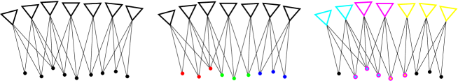
Figure 1: A block (left) is split into sub-blocks with unique points according to Zhang et al. (2017) (center) and with unambiguous cameras – our case (right). The colored points on the right are the tie points contained in different sub-blocks.

$$(\mathbf{P})^{t+1},$$

$$(\mathbf{X}^{l})^{t+1} = \arg\min_{\mathbf{P},\mathbf{X}^{l}}\Bigl{(}f_{l}((\mathbf{P})^{t},(\mathbf{X}^{l})^{t},\mathbf{x})+\frac{\rho}{2}\|(\mathbf{X}^{l})^{t}-(\mathbf{X})^{t}+(\tilde{\mathbf{X}}^{l})^{t}\|_{2}^{2}\Bigr{)}$$ (11)

$$(\mathbf{X}_{j})^{t+1} = \frac{1}{L}\sum\limits_{l=1}^{L}(\mathbf{X}_{j}^{l})^{t+1}$$ (12)

$$(\tilde{\mathbf{X}}_{j}^{l})^{t+1} = (\tilde{\mathbf{X}}_{j}^{l})^{t}+(\mathbf{X}_{j}^{l})^{t+1}-(\mathbf{X}_{j})^{t+1}\;.$$ (13)

In (11) cameras as well as points are jointly optimized, but separately for each sub-block. (12) averages the coordinates of the TPs and, finally, in (13) an improvement is computed for each of the 3D points for every sub-block to drive the iterative solution.

In (Zhang et al., 2017) the convergence of the consensus is analyzed for the case where the points are unique in the sub-blocks and there can be separate estimates for the cameras if they picture 3D points in more than one sub-block. There are two findings: The first is not relevant for our case as it pertains to the cameras, particularly their rotation. The second is concerned with the translation of the camera and the 3D points which is relevant also for our case. Here, the condition for convergence consists in that the 3D points should not be extremely close to the cameras, which can be safely assumed to hold for SfM problems (Zhang et al., 2017), i.e., in our case.

5 Extended Consensus-Based Bundle Adjustment

When looking more closely at (11) one can see that it is actually very similar to bundle adjustment using stochastic (ground) control points for absolute pose estimation / orientation. In our case, the role of the control points is taken by the TPs which link two or more sub-blocks and we extend $f$ by weighting in the form of the inverse of the approximate covariance matrix of the measurements $\mathbf{C}^{-1}_{\mathbf{x}}$ as in (5)

$$\arg\min_{\mathbf{P},\mathbf{X}}\Bigl{(}f(\mathbf{P},\mathbf{X},\mathbf{x},\mathbf{C}^{-1}_{\mathbf{x}})+\|\mathbf{X}-\mathbf{X}_{\mbox{\scriptsize TP}}\|_{\mathbf{W}_{\mbox{\tiny TP}}}\Bigr{)}\;.$$ (14)

Opposed to (11), here the relative weighting between $f(\mathbf{P},\mathbf{X},\mathbf{x},\mathbf{C}^{-1}_{\mathbf{x}})$ and the distance between the 3D points $\mathbf{X}_{j}$ and the TPs is done by a weight matrix $\mathbf{W}_{\mbox{\tiny TP}}$. The latter can be used to introduce the information on the global 3D points common to different sub-blocks, i.e., TPs, in a more detailed way. We again note that we split up the cameras unambiguously, i.e., every camera is just contained in one sub-block, while the 3D points can be visible in more than one sub-block. Written in the way of (11) with $\mathbf{C}^{-1}_{(X_{\mbox{\tiny TP}})^{t}}$ the inverse of the covariance information for a 3D point it reads

$$(\mathbf{P})^{t+1} = \arg\min_{\mathbf{P},\mathbf{X}^{l}}\Bigl{(}f_{l}((\mathbf{P})^{t},(\mathbf{X}^{l})^{t},\mathbf{x},\mathbf{C}^{-1}_{\mathbf{x}})+\|(\mathbf{X}^{l})^{t}-(\mathbf{X}_{\mbox{\scriptsize TP}})^{t}\|_{\mathbf{C}^{-1}_{(\mathbf{X}_{\mbox{\tiny TP}})^{t}}}\Bigr{)}\;.$$ (15)

When experimenting with the above ADMM scheme, we found similar to Ayeni (1980) that a relative large number of iterations is needed and we thought about ways to improve convergence.

Bringing together both above issues led to the idea to replace the averaging of the corresponding 3D points in different sub-blocks in (12) by adjustment / intersection / triangulation just for the TPs: I.e., we take the cameras from the different sub-blocks of (15) as fixed and just optimize the position of the TPs obtaining by this means also their covariance information $\mathbf{C}_{(\mathbf{X}_{\mbox{\tiny TP}_{j}})^{t}}$ needed for (15)

$$(\mathbf{X}_{\mbox{\scriptsize TP}_{j}})^{t+1},\mathbf{C}_{(\mathbf{X}_{\mbox{\tiny TP}_{j}})^{t+1}} = \arg\min_{\mathbf{X}_{j}}f_{j}((\mathbf{P})^{t+1},(\mathbf{X}_{j})^{t},\mathbf{x}_{k},\mathbf{C}^{-1}_{\mathbf{x}_{k}})\;.$$ (16)

Overall, we just switch between (15) and (16) without the need to compute an improvement as in (13). This has two basic advantages:

1. We found that the estimated $(\mathbf{X}_{\mbox{\scriptsize TP}_{j}})^{t+1}$ from (16) lead to a much better convergence than the averages from (12).

2. One obtains an estimate of the covariance matrix $\mathbf{C}_{(\mathbf{X}_{\mbox{\tiny TP}_{j}})^{t+1}}$ which can be readily plugged into (14) without any fiddling with the penalty parameter $\rho$, as the covariance matrix is inherently scaled correctly.

Intuitively, the proof in (Zhang et al., 2017) should also apply here as it is a refined version of the above ADMM scheme. Practically, we found a very good convergence behavior of the above scheme as presented in detail below in Section 6.

Additionally, the above scheme is related to resection / intersection schemes such as (Bleser et al., 2007, Mitra and Chellappa, 2008, Pritt, 2014, Hänsch et al., 2016), where one switches between optimizing individual points and cameras. This can also be regarded as Gauss-Seidel iteration (Ayeni, 1980, Wang and Clarke, 2001).

For parallel processing, the above schemes have to distribute all points and all cameras for each iteration. Opposed to this, for the computation of (16) we just have to distribute all cameras and the TPs. Additionally, as demonstrated below in the experiments by extending the number of sub-blocks and thereby reducing the number of cameras in each sub-block, the convergence rate is much better for larger sub-blocks. Particularly, we found that one should adapt the number of sub-blocks to the number of threads available on a computer.

Finally, we note the link to Jeong et al. (2012), which employ “embedded point iterations” to speed up the convergence of their method for bundle adjustment. As we similarly optimize the point positions independently, we can also expect a corresponding speed-up.

5.1 Refined Re-Weighting

The covariance for all cameras is computed by means of (16). As we use $\mathbf{C}_{(\mathbf{X}_{\mbox{\tiny TP}_{j}})^{t+1}}$ for weighting the TPs in the sub-blocks, it seems reasonable to compute this per sub-block. Particularly, the idea is to use per sub-block only the information from all cameras in all sub-blocks besides the current, i.e., $L\setminus l$.

While we formally work with the inverse of the covariance matrix, we note that the covariance matrix is itself the inverse of the normal equations which are derived from the Jacobian $\mathbf{A}$ using as weight the inverse of the approximate covariance matrix of the measurements for the 3D point $j$ $\mathbf{C}_{j}^{-1}$, cf. (5). Thus, we skip the double inverse and use as refined weight matrix the normal equations reduced to those cameras which are not included in sub-block $l$

$$\mathbf{C}^{-1}_{(\mathbf{X}^{l}_{\mbox{\tiny TP}_{j}})^{t+1}} = (\mathbf{A}_{j}^{L\setminus l})^{\mbox{\sf\scriptsize T}}(\mathbf{C}_{j}^{L\setminus l})^{-1}(\mathbf{A}_{j}^{L\setminus l})\;.$$ (17)

The above just applies to the calculation of the weight matrix. The computation of the point position $(\mathbf{X}_{\mbox{\scriptsize TP}_{j}})^{t+1}$ is based on all cameras in all sub-blocks in which the point is visible.

5.2 Sub-Block Construction by Means of Graph Partitioning

Our parallelization builds on sub-blocks. Basically, for larger blocks one usually employs as many sub-blocks as threads available on a computer. Yet, below a certain block size it is more efficient to adjust the block serially without parallelization.

Concerning the sub-blocks it is important to obtain a balanced load of the threads particularly concerning computation time. Additionally, it is helpful when the sub-blocks do not have too many TPs to reduce the computation in (16) and the effort for the exchange of the information concerning the 3D points and cameras between (15) and (16).

Particularly, we have defined this as a graph partitioning problem of the visibility graph and similarly as Ni et al. (2007) we use METIS’ (Karypis and Kumar, 1998) 5.1 multilevel recursive bisection graph partitioning algorithm to solve it.

Configuring METIS proved difficult and could only be done empirically. Basically, the computational complexity for bundle adjustment of a sub-block is related to the third power of the number of cameras and the number of observations in the sub-block. The first issue is that METIS does not allow for a constraint on the number of elements in a sub-block. Additionally, because we use CG for solving and as in most larger sub-blocks far from all cameras are directly related by observations, the computational complexity is well below the third power of the number of cameras.

We empirically found that weighting each node of METIS, i.e., camera, by the cubic root of the sum of the number of observations of all cameras for all 3D points a camera “sees” gives the best result in terms of computation time. Intuitively, by this means we implicitly model that the computational complexity for a camera is not only related to the number of 3D points it has imaged, but also to how many cameras it is related to, implicitly given by the number of observations for the 3D point.

5.3 Robust Estimation

In numerous experiments we have found that a very simple approach works very well for robust estimation given the results of a SfM pipeline such as (Mayer et al., 2012) based on Random Sample Consensus – RANSAC (Fischler and Bolles, 1981). The approach is based on normalized weighted squared residuals $\overline{v_{k}}^{2}=\frac{\mathbf{v}_{k}^{\mbox{\sf\scriptsize T}}\mathbf{C}_{\mathbf{x}_{k}}\mathbf{v}_{k}}{\sigma_{0}^{2}}$, i.e., the weighted squared residual divided by the variance of the weighted image measurements

$$\sigma_{0}^{2}=\frac{\sum_{k}{\mathbf{v}_{k}^{\mbox{\sf\scriptsize T}}\mathbf{C}_{\mathbf{x}_{k}}\mathbf{v}_{k}}}{redundancy}\;,$$ (18)

and works in two steps:

• After basic convergence of the adjustment, the observations for which $\overline{v_{k}}$ is beyond a certain threshold $t_{v}$ (empirically set to 3) are weighted down strongly by 1.e-4.

• After finishing the iteration, the corresponding observations are deleted. If this means that a 3D point is observed in only one camera, it is completely eliminated.

We had initially (Mayer et al., 2012) used the variance of individual weighted squared residuals $\sigma_{\mathbf{v}_{k}}^{2}$ instead of $\sigma_{0}^{2}$, but found that this often lacks robustness. The latter is also the case if one estimates $\sigma_{0}$ according to (18). We, thus, have switched to estimating $\sigma_{0}$ for robust estimation by means of the Median Absolute Deviation (MAD) multiplied by the factor 1.4826 under the assumption that the variance is normally distributed. Experimentally this gives rather robust results, particularly when the estimation is done per camera, which is not only faster but also more meaningful especially when the cameras are of a different type, possibly with a rather different image size.

While it would be conceptually useful to employ only one consistent robust estimation scheme, different schemes are used in the serial and the parallel case. This basically accounts for the fact that depending on the block structure a substantial number of 3D points might be TPs and visible in a larger number of sub-blocks. When a point is seen in a sub-block by only very few cameras, a reliable detection of an outlier is difficult.

Thus, we decided to conduct robust estimation for the parallel case by robust weighting during the estimation of the 3D points in the intersection part, because there all cameras a point is seen in are involved. Additionally, complete 3D points are eliminated instead of just individual image observations. As shown later in the experiments in Section 6.5, the difference between the effectiveness of the parallel and the serial version is relatively small, particularly when $t_{v}$ is set to 4 in the parallel case instead of 3 in the serial case as found by numerous experiments.

5.4 Implementation Details

Our implementation is influenced in many ways by Jeong et al. (2012). We use the Schur complement to obtain the RCS which is solved by preconditioned CG. By employing outer products we accumulate the 3D points directly in the RCS and avoid intermediate matrices. We also follow Jeong et al. (2012) by utilizing block-based Jacobi preconditioning, i.e., we use the inverses of the diagonal blocks for preconditioning. Similarly as Jeong et al. (2012) we employ a three parameter Rodriguez representation but limited to the incremental rotation during adjustment, avoiding problems with rotations close to 180^∘. For the LM algorithm we also multiply the diagonal of the normal equations $\mathbf{N}$ (4) with the damping factor, i.e., $\mathbf{N}_{aug}=\mathbf{N}+\lambda\mathbf{I}\;\mbox{diag}\{\mathbf{N}\}$.

When developing and later improving (Mayer et al., 2012) we found in many experiments that setting $\lambda$ to 1.e-3 or 1.e-4 is sufficient (in this paper it is set to 1.e-4, but for wide-baseline settings it is advantageous to set it to 1.e-3). Only for finally estimating covariance information—if needed—we set $\lambda$ to 1.e-6 after initial convergence. For the determination of convergence we compare the best reprojection error obtained so far with the current reprojection error. If the ratio is below 1.01, we stop the iteration. To deal with convergence problems particularly in the first round of iterations, we allow for one iteration without an improvement of more than 1.01.

We acknowledge that setting $\lambda$ to 1.e-4 leads to biased results if covariance matrices are estimated. Yet, we note that we found this relatively high value necessary to obtain convergence for difficult datasets. A solution could be adapting $\lambda$ as in (Jeong et al., 2012), but that means another solution of the normal equations with the corresponding effort. Revisiting this issue could be part of future work although our current experiences do not point to significant deficits in this respect.

We obtain basic robustness concerning far-away points as well as outliers by throwing out the very few points where the intersection of a 3D point does not converge.

We finally note that our implementation which is based on METIS (Karypis and Kumar, 1998) and the linear algebra library Eigen is available on GitHub: https://github.com/helmayer/RPBA

6 Experiments

As a baseline we compare our (extended) approach to PBA – Parallel Bundle Adjustment (Wu et al., 2011), but the main focus is on the comparison to the (plain) consensus-based approach introduced in Section 4. For the experiments we use a computer with 12 cores, 24 threads and 64 GB of memory running Linux.

We use the data sets Final 13682 and Final 961 introduced in (Agarwal et al., 2010b) and Dino from (Seitz et al., 2006) as well as a Simulated data set. The latter is in the form of a “traditional” aerial block with 50 strips and 400 cameras per strip, 0.6 endlap, 0.2 sidelap and around 100 statistically distributed points per camera but only in the overlap area, i.e., 20,000 cameras and 1,861,000 3D points. We added 1.0 pixels Gaussian noise to the image observations and perturb the camera parameters by 0.0001 radians in the angles and $0.1$ units in the coordinates, leading to an initial average back projection error of about 30 pixels.

data set	# cameras	# points	# observations	# parameters
				for cameras
Final 13682	13,682	4,456,117	57,973,736	n * (6 + 2)
Final 961	961	187,103	3,385,950	n * (6 + 2)
Dino	363	37,796	423,718	n * 6 + 7
Simulated	50 $\times$ 400	1,861,000	12,001,562	n * 6

Table 1: Characteristics of the data sets

For the two Final data sets we estimate the camera constant / principal distance / focal length as well as the first (quadratic) parameter of the radial distortion together with the camera poses separately for each camera as has been done in other experiments with these data sets and is also standard with PBA. For the Simulated data set we just compute the camera poses, but for Dino we estimate the camera poses as well as a joint calibration matrix and quadratic as well as quartic radial distortion.

As due to reasons of efficiency it is not meaningful to work with too small sub-blocks, we limited their minimum size for the experiments to an empirically found value of 70 cameras.

Our approach used in the experiments is the extended consensus-based adjustment approach introduced in the preceding section including the refined re-weighting of Section 5.1. It is called the “extended approach” for the remainder of this paper. Compared to this, we call the consensus-based approach from Section 4 the “plain approach”. An overview of all employed approaches is given in Table 2.

extended approach	Section 5 incl. refined re-weighting (Section 5.1)
plain approach	Section 4
PBA	(Wu et al., 2011)

Table 2: Overview of the approaches

6.1 Sub-Block Sizes and Computation Times

In this section we give a visual impression of the data sets as well as how they are split into sub-blocks by METIS (Karypis and Kumar, 1998) via the graph partitioning approach introduced in Section 5.2.

Figure 2 shows how the Simulated data set with 50 strips is split into 2 and 24 sub-blocks. In the second case, this corresponds to the number of physical threads of our processor. One can see that the algorithm splits the data set into compact, mostly contiguous sub-blocks. The latter is not so obvious for the two Final data sets (cf. Figures 3 and 4), because the images are strongly overlapping as most try to picture the same part of the scene although from different view points. While for Final 961 nearly no structure can be seen, due to its much larger size, Final 13682 shows some more contiguous areas (e.g., the sub-block marked in yellow). Finally, Figure 5 gives an impression of the data set Dino, which is used to demonstrate the efficiency of our approach for robust estimation in Section 6.5. As it consists of merely 363 cameras, it is split into only 5 sub-blocks due to the minimum sub-block size of 70. Also here many cameras see the same area of the scene (there are points projected into more than 90 cameras), but still the sub-blocks are mostly contiguous.

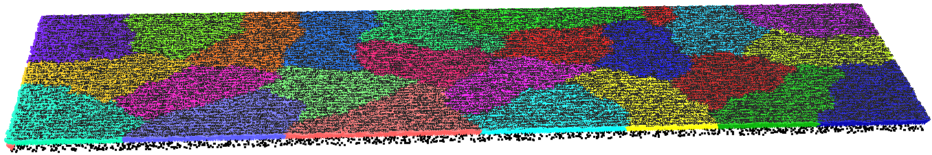
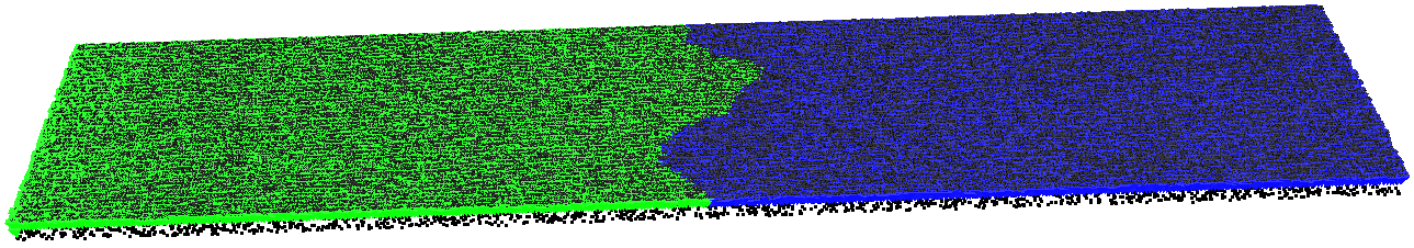
Figure 2: Simulated block with 50 strips and 400 cameras per strip split by METIS into 24 sub-blocks (top) and 2 sub-blocks (bottom), marked by different colors.

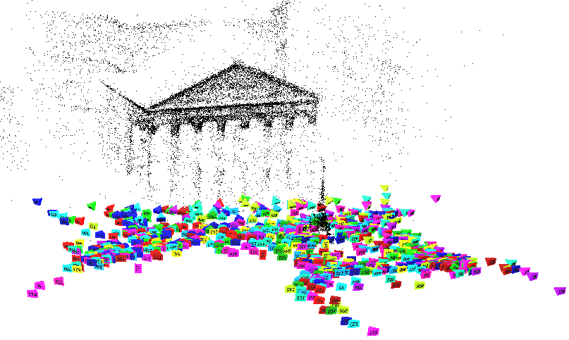
Figure 3: Final 961 from (Agarwal et al., 2010b) split by METIS into 14 sub-blocks marked by different colors.

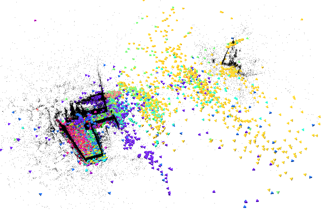
Figure 4: Final 13682 from (Agarwal et al., 2010b) split by METIS into 24 sub-blocks marked by different colors.

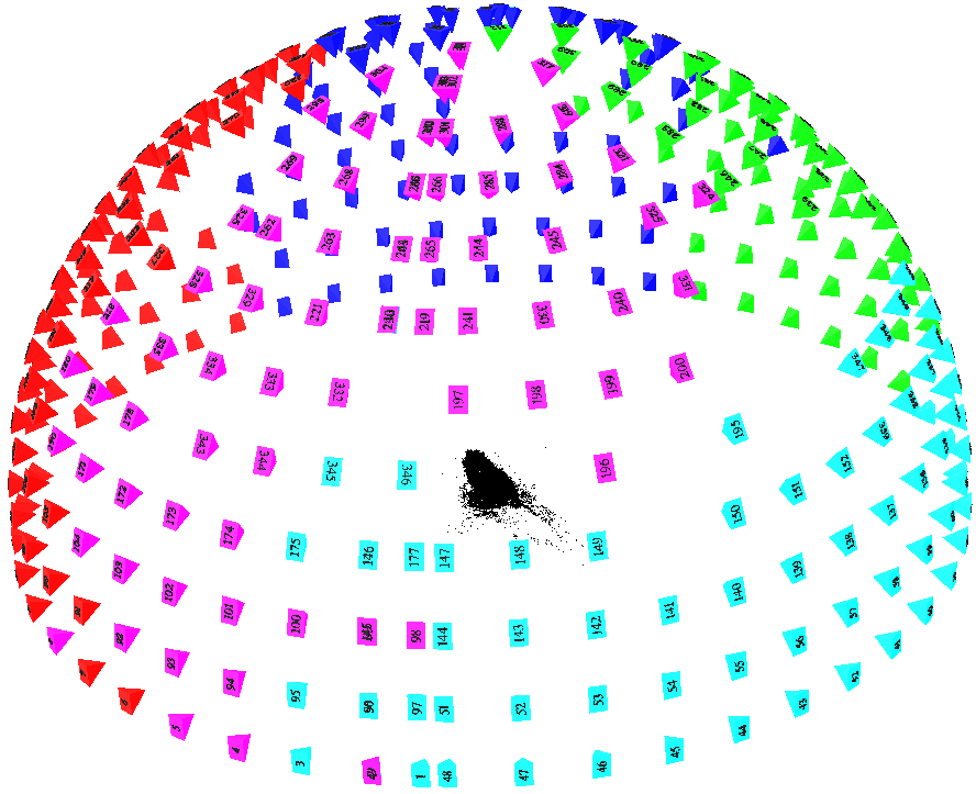
Figure 5: Data set Dino from (Seitz et al., 2006) split by METIS into 5 sub-blocks marked by different colors.

In Figure 6 we give a comparison between the sizes of the sub-blocks and the overall computation times for all iterations ordered according to the sub-block sizes for Final 13682. One can see that there is no direct relation between the two: larger blocks might have a smaller computation time than much smaller blocks. We assume that this is due to the different neighborhood structure and, thus, sparsity of the individual sub-blocks. Overall, this is the optimum result concerning the computation time we found by numerous experiments particularly for this large data set. As outlined in Section 5.2, the basic reason why we could not do better has been that for the graph-based METIS we could not define constraints on the overall number of cameras and observations per sub-block. We found similar distributions also for numerous other data sets.

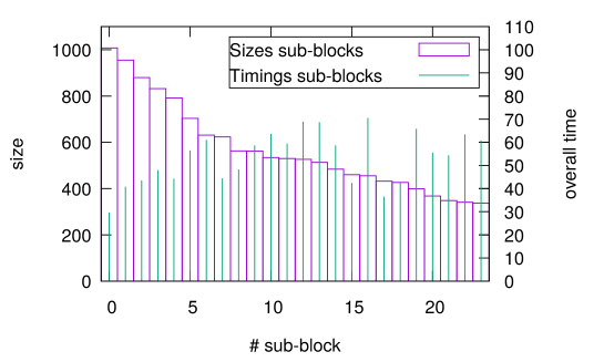
Figure 6: Sizes of the sub-blocks (box) ordered according to size in comparison with the overall time per sub-block/thread (vertical line) for data set Final 13682.

6.2 Convergence Behavior Depending on the Number of Threads

This section gives a comparison of the convergence behavior and corresponding timings for different numbers of threads for the extended approach based on the data set Final 13682. Convergence is described according to the behavior of the average standard deviation of the weighted image measurements $\sigma_{0}$ (18) which can be interpreted as the average error of the weighted image measurements. The latter holds because we use normalized weights which are 1 on average. This is trivial for the two Final datasets and the Simulated dataset were no weights are given and they are, thus, simply set to 1. For Dino we determine individual weights by means of least squares matching and then normalize them.

Figure 7 shows that there is not necessarily convergence for all iterations, an iteration consisting of one solution of equations (15) and (16) each. Particularly in the first couple of iterations it is possible that coordinates for joint 3D points in different sub-blocks can be quite different leading to large errors. Yet, as shown in Table 3, in the end the differences between the various solutions are very small in terms of $\sigma_{0}$.

Overall, the convergence is faster for a smaller number of sub-blocks, which is to be expected as there are less common 3D points which have to be adjusted by means of the interaction between bundle adjustment for the sub-blocks and intersection of the 3D points. On the other hand, the convergence is more smooth, particularly without any rise, for a larger number of sub-blocks. Finally, please note that the fastest solution is obtained for the physical number of threads on the employed computer, namely 24. While for a smaller number not all the computing power is used, a larger number implies more not really efficient iterations with bundle adjustment of sub-blocks and intersection of the 3D points. It is, thus, recommended to split the block in as many sub-blocks as physical threads are available as long as the sub-blocks do not become too small and, thus, the overhead for parallel computing becomes too large.

threads	# iterations	$\sigma_{0}$ [pixel]	time [sec]	convergence $\sigma_{0}$
6	6	1.006	473	2.91 1.14 1.16 1.020 1.010
12	6	1.008	219	2.91 1.15 1.14 1.019 1.012
24	6	1.014	149	2.91 1.16 1.13 1.043 1.018
48	7	1.014	212	2.91 1.19 1.12 1.033 1.022 1.017
96	7	1.016	392	2.91 1.21 1.11 1.042 1.025 1.020

Table 3: Convergence of Final 13682 from (Agarwal et al., 2010b) for different numbers of threads. There are 24 threads available by the hardware.

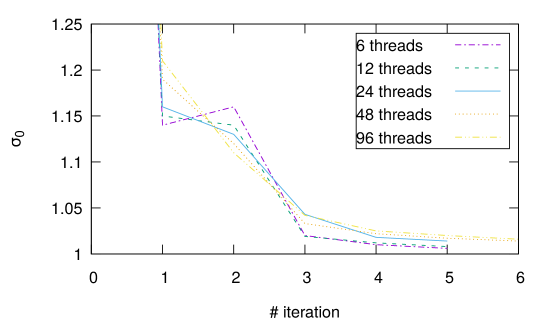
Figure 7: Convergence of Final 13682 for different numbers of threads.

6.3 Comparison to PBA and Between Different Variants of Consensus

In this section we compare our extended approach (cf. Table 2) with the baseline PBA (Wu et al., 2011) in its current version (master-PBA – http://sourceforge.net/PBA-master) as well as our implementation of the plain approach based on the standard deviation / average error of the weighted image measurements $\sigma_{0}$ (cf. preceding section).

Concerning PBA it was not easy to process the Final 13682 data set. Only by switching to “measurement distortion” instead of “projection distortion” we could obtain a solution which was not extremely much worse than for the other two approaches. On the other hand, the solution by PBA for Final 961 is very close to the solution obtained by our extended consensus. The same is true for the Simulated data set. We let PBA write its solution with the improved parameters into a file and used our software to consistently compute $\sigma_{0}$.

For the plain approach we had to fix a couple of parameters. Of biggest importance we found to be the parameter $\rho$ (cf. Section 4 equation (7)). As recommended in (Zhang et al., 2017), we modify $\rho$ by multiplying it with a factor $1.01$ for each iteration. The latter is the same for all data sets. For $\rho$ itself different values were necessary for different data sets. For Final 13682 and 961 we set $\rho$ to 1000, for the Simulated data set to 200. We additionally found that the plain approach could not deal with a few very far-away as well as with outlier points. To deal with this, we included a filter throwing out points with very large coordinate values ($>$ 1.e10) as well as a large distance between projected and measured points. Yet, this only applied to a few points.

Table 4 summarizes the results for the data sets Final 13682 and 961. One can see that our extended approach is fastest and produces the best results for Final 13682. The result is very similar to the result of PBA for Final 961. As discussed above, we could not find any setting for the parameters for PBA which gave a better result for Final 13682. Concerning the comparison of the plain and the extended approach, the latter is not only faster, but it produces also results of a higher accuracy in much fewer iterations. Figure 8 gives a graphical impression of the convergence behavior. It shows that due to the use of the additional information in the form of the covariance matrix of the TPs as well as due to the replacement of the simple averaging by triangulation based on adjustment, the extended approach converges considerably faster and reaches a lower value for $\sigma_{0}$.

data set	approach	# iterations	$\sigma_{0}$ [pixel]	time [sec]
13682	plain	18	1.051	443
	extended	6	1.014	149
	PBA		1.123	175
961	plain	17	1.139	13.3
	extended	6	1.089	7.4
	PBA		1.088	18.2

Table 4: Comparison of the plain and the extended approach as well as PBA (Wu et al., 2011) for Final 13682 and 961.

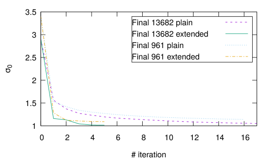
Figure 8: Convergence Final 13682 and 961 for plain and extended approach (all on 24 threads).

For the Simulated data set all approaches work relatively well (cf. Table 5). We first note that the differences of the obtained $\sigma_{0}$ can basically be neglected. Both, the plain approach and PBA are considerably slower than the extended approach. We have also compared the results for the extended approach for different numbers of threads. As above for Final 13682, one can see that we achieve the optimum speed for the physical number of threads (24) of the computer used for the experiments.

approach / threads	# iterations	$\sigma_{0}$ [pixel]	time [sec]
plain 24	8	1.0008	27.2
extended 1		0.9978	210
extended 2	4	1.0005	36.7
extended 3	4	1.0005	27.3
extended 6	4	1.0006	16.9
extended 12	4	1.0007	12.9
extended 24	4	1.0008	12.4
extended 48	4	1.0008	16.3
extended 96	4	1.0010	29.1
PBA 24		1.0002	36.4

Table 5: Comparison of plain and extended approach as well as PBA for the Simulated data set. For the extended approach (center rows) the results for different numbers of threads are given. 24 is the number of physical threads.

6.4 Ablation Study

This section quantifies the influence of our contributions based on the Simulated data set as well as Final 961 and 13682. In Table 6 we compare the result for the complete extended approach with simplified versions as well as with one version of the plain approach improved by means of the refined re-weighting of Section 5.1, but without the intersection of the 3D points.

To quantify the influence of the refined re-weighting introduced in Section 5.1 and included in the complete system, we compare it by weighting just by means of a scalar and by weighting taking into account all cameras instead of just those in which a 3D point in a certain sub-block is not visible as in Section 5.1. For weighting by means of a scalar, we use the same scheme as for the plain approach, yet, we still compute the new point estimates by means of intersection / adjustment of the 3D points. We replace the full covariance matrix per point by a diagonal matrix where all elements are the same and correspond to the $\rho$ of the plain approach.

The full extended approach gives the best results concerning the number of iterations and computation time. Weighting with all cameras gives a little bit worse results. The accuracy is slightly lower, the number of iterations as well as the time is a little bit higher. If one substitutes the inverse covariance matrix by a scalar, the accuracy particularly for Final 961 becomes substantially lower even though the number of iterations and the computation time is similar to the (full) extended approach. For Final 13682 the result is worse and the number of iterations as well as the computation time are higher.

On the other hand, the results for the plain approach extended by the refined re-weighting of Section 5.1 show that the plain approach can be improved by the refined re-weighting. Yet, the result for Final 13682 makes clear that the 3D intersection of the points is essential and refined re-weighting is not enough. While the approach converged very fast to a $\sigma_{0}$ of 1.04 pixels, it diverged after this point and we did not find any means to fix this.

extended approach	Simulated	Final 961	Final 13682
# iterations	4	6	6
$\sigma_{0}$	1.0008	1.089	1.014
time [secs]	12.4	7.4	149
extended: weighting with all cameras
# iterations	4	7	8
$\sigma_{0}$	1.0008	1.101	1.020
time [secs]	13.1	8.2	171
extended: weighting with scalar
# iterations	4	6	7
$\sigma_{0}$	1.0009	1.157	1.044
time [secs]	14.0	7.4	181
plain: refined re-weighting of Section 5.1
# iterations	4	8	4 (diverging)
$\sigma_{0}$	1.0009	1.124	1.055
time [secs]	15.2	10.4	(132)

Table 6: Results for different variants of the extended (original: top row) and the plain approach.

6.5 Effectiveness of Robust Estimation

Concerning our approach for robust estimation introduced in Section 5.3, we present two different types of experiments: The first gives an impression of the improvement of accuracy possible by means of robust estimation as well as what happens if there are actually no outliers as for the Simulated data set. The second type of experiments compares multiple use of our parallel robust (extended) approach with standard serial bundle adjustment using just a single thread. If the parallel approach would be significantly worse, the multiple use should lead to substantially different final results.

For the former type of experiments, Table 7 presents the results. The improvements by means of robust estimation are assessed by two means: First, based on the standard deviation / average error of the weighted image measurements $\sigma_{0}$ and second based on the variances of the parameters. For the latter, we give mean and standard deviation as well as the median of the ratios of the variances for the parameters estimated without and with robust estimation.

For the Simulated data set for which we added a noise of 1.0 pixel a very good approximation of 1.0006 pixels is obtained. Of about 12 Million observations less than 600 are eliminated, i.e., 0.005%. This verifies that our robust parallel approach does not (nearly) randomly delete points.

The results for Final 961 and 13682 show that the accuracy could be improved by a factor of 1.5 by eliminating less than 3% of the points. From other experiments we know that these are typical values. The number of iterations and the computation time approximately doubles for the robust case. For Final 961, the result for the parallel approach is similar to that of the serial approach, but the computation time is much lower.

The ratio of the variances match the ratio of the $\sigma_{0}$ for the serial estimation result of Final 961, the only data set for which variances could be calculated due to restrictions of the memory size (64 GB were not enough). For parallel robust estimation, the ratios of the variances fluctuate notably, but the average and particularly the median of the ratios is similar to the ratio of the $\sigma_{0}$, meaning that not only the average error but also the variances of the parameters have improved (at least on average).

Parallel	Simulated	Final 961	Final 13682
# threads	24	14	24
# iterations	5	11	10
$\sigma_{0}$ [pixel] not robust	1.0008	1.089	1.014
# observations	12,001,562	3,385,950	57,973,736
# deleted (%)	576 (0.005%)	97,894 (2.9%)	1,503,098 (2.6%)
$\sigma_{0}$ [pixel] final	1.0006	0.721	0.706
Ratio $\sigma_{0}$ not robust / final	0.9998	0.662	0.696
Ratio variances mean	0.9999 $\pm$ 0.005	0.793 $\pm$ 0.36	0.744 $\pm$ 0.27
Ratio variances median	0.9996	0.733	0.721
time [sec]	16.7	14.9	266
Serial
# deleted (%)	0 (0.%)	98,632 (2.9%)	–
$\sigma_{0}$ [pixel] final	1.0010	0.706	–
Ratio $\sigma_{0}$ not robust / final	1.0002	0.648	–
Ratio variances mean	–	0.627 $\pm$ 0.007	–
Ratio variances median	–	0.630	–
time [sec]	382	391	–

Table 7: Results for parallel robust estimation for different data sets. For Final 961 only 14 threads are used as the minimum number of cameras per sub-block/thread is set to 70. Because of lack of memory, no serial solution could be computed for Final 13682 and no variance information for the serial solution for the Simulated dataset (–).

For efficiently testing the effectiveness of our approach for robust estimation, we use the data set Dino and a version of our SfM software which repeatedly adds small blocks to large blocks leading to many bundle adjustments. Although we limited the minimum number of cameras per sub-block / thread to 70 cameras, we still could use the parallel bundle adjustment 31 times of overall 361 adjustments with between 2 and 5 threads (Dino consists of 363 cameras).

Table 8 gives the results for serial robust bundle adjustment as well as for the robust version of our extended approach. We, particularly, compare the accuracy obtained before the final (serial – as benchmark) bundle adjustment, the accuracy after the final bundle adjustment, the number of points obtained and the time it takes to merge the block. One can see that the results apart from the computation time are actually very similar. This is confirmed by Table 9 which shows that the ratios of the variances of the parameters for the parallel and the serial solution are close to one and, thus, the variances are rather similar.

approach	$\sigma_{0}$ [pixel] before	$\sigma_{0}$ [pixel] final	# observations	time [sec]
	final adjustment			overall
serial	3.4	0.41	423,612	155.6
parallel	3.0	0.40	424,418	53.1

Table 8: Comparison of the characteristics of the results for data set Dino processed by serial and parallel bundle adjustment, the latter with 2 to 5 threads in 31 of 361 adjustments (as the minimum number of cameras per thread is set to 70). The timings additionally contain a constant part for least-squares matching.

min	max	median	mean
0.91	1.16	0.981	0.983 $\pm$ 0.023

Table 9: Statistics of ratios of variances of parallel and serial solution for Dino.

To present the results a little bit more in detail, Figure 9 gives a comparison of the number of points projected in a certain number of cameras. The more points are projected in as many cameras as possible, the better the block stability becomes, as they tie the cameras to each other. The comparison shows that the results of the serial and the parallel approach are very similar. Together with the above comparison of the accuracies and final variances, number of points and computation time this demonstrates that the robust extended approach can be a fast replacement for standard serial robust bundle adjustment.

Figure 9: Distribution of points projected in multiple cameras for data set Dino processed by serial and parallel robust bundle adjustment.

7 Conclusion

Extending recent consensus-based approaches, we present means to efficiently exploit the characteristics of modern parallel computers for robust bundle adjustment. While resection / intersection schemes have a weak convergence behavior and normal bundle adjustment needs too many resources and is not inherently parallel, our scheme allows to make use of each thread independently and still obtain a high quality result in only a few iterations.

The latter distinguishes it from competing recent consensus-based approaches, although there are just two big differences between their work and ours:

• They average the 3D point coordinates and use a penalty parameter $\rho$.

• We determine the points by forward intersection and get rid of the dataset-dependent penalty parameter $\rho$ by replacing it by the covariance information for the 3D points. Thus, no parameter tuning is necessary.

Interestingly, Jeong et al. (2012) have also come to the conclusion that adjusting 3D points can be particularly useful and use “embedded point iterations” as an important part of their work.

Future work could comprise an improved rescaling of the dampener in the Levenberg-Marquardt algorithm as recommended in (Jeong et al., 2012) by means of trust region control (Lourakis and Argyros, 2005). Even though splitting up the block in sub-blocks reduces efficiency issues while solving the reduced camera system (RCS) considerably, for extremely large (sub-)blocks still an ordering of the variables to minimize the amount of fill-in during the solution could be helpful. For this, exact minimum degree ordering as used in (Jeong et al., 2012) could be an option.

Concerning robust estimation, it might be possible to just detected the outliers during intersection and then forward this information to be employed in resection. In addition to the implementation effort it will still not be as statistically efficient as serial robust estimation, because each sub-block contains at least for a certain fraction of the 3D points only parts of the image observations.

Appendix A Bibliography

References

- Ackermann (1962) F. Ackermann. Some Results of an Investigation into the Theoretical Precision of Planimetric Block-Adjustment. Photogrammetria, 19(8):505–509, 1962.
- Agarwal et al. (2014) P. Agarwal, W. Burgard, and C. Stachniss. Helmert’s and Bowie’s Geodetic Mapping Methods and Their Relation to Graph-based SLAM. In International Conference on Robotics and Automation, 2014.
- Agarwal et al. (2009) S. Agarwal, N. Snavely, I. Simon, S. Seitz, and R. Szeliski. Building Rome in a Day. In Twelfth International Conference on Computer Vision, pages 72–79, 2009.
- Agarwal et al. (2010a) S. Agarwal, K. Mierle, and Others. Ceres solver. http://ceres-solver.org, 2010a.
- Agarwal et al. (2010b) S. Agarwal, N. Snavely, S. Seitz, and R. Szeliski. Bundle Adjustment in the Large. In Eleventh European Conference on Computer Vision, pages 29–42, 2010b.
- Ayeni (1980) O. Ayeni. Phototriangulation: A Review and a Bibliography. In International Archives of Photogrammetry, volume (23) B9, pages 313–357, 1980.
- Balasalle (2018) J. Balasalle. Parallel Bundle Adjustment of High Resolution Satellite Imagery. Dissertation, University of Colorado Boulder, 2018.
- Bertsekas and Tsitsiklis (1989) D. Bertsekas and J. Tsitsiklis. Parallel and Distributed Computation: Numerical Methods, volume 23. Prentice-Hall International, Englewood Cliffs, USA, 1989.
- Bleser et al. (2007) G. Bleser, M. Becker, and D. Stricker. Real-time Vision-based Tracking and Reconstruction. Journal of Real-Time Image Processing, 2(2–3):161–175, 2007.
- Brown (1958) D. Brown. A Solution to the General Problem of Multiple Station Analytical Streotriangulation. Technical Report AFMTC TR 58-8, Patrick Airforce Base, Florida, 1958.
- Brown (1976) D. Brown. The Bundle Adjustment – Progress and Prospects. In International Archives of Photogrammetry, volume (21) 3, pages 1–33, 1976.
- Carlone et al. (2014) L. Carlone, P. Alcantarilla, H.-P. Chiu, Z. Kira, and F. Dellaert. Mining Structure Fragments for Smart Bundle Adjustment. In British Machine Vision Conference, pages 1–12, 2014.
- Eriksson et al. (2016) A. Eriksson, J. Bastian, T.-J. Chin, and M. Isaksson. A Consensus-Based Framework for Distributed Bundle Adjustment. In Computer Vision and Pattern Recognition, pages 1754–1762, 2016.
- Fischler and Bolles (1981) M. Fischler and R. Bolles. Random Sample Consensus: A Paradigm for Model Fitting with Applications to Image Analysis and Automated Cartography. Communications of the ACM, 24(6):381–395, 1981.
- Förstner and Wrobel (2016) W. Förstner and B. P. Wrobel. Photogrammetric Computer Vision. Springer, Cham, Switzerland, 2016.
- Frahm et al. (2010) J.-M. Frahm, D. Gallup, T. Johnson, R. Raguram, C. Wu, Y.-H. Jen, E. Dunn, B. Clipp, S. Lazebnik, and M. Pollefeys. Building Rome on a Cloudless Day. In Eleventh European Conference on Computer Vision, volume IV, pages 368–381, 2010.
- Fusiello and Crosilla (2015) A. Fusiello and F. Crosilla. Solving Bundle Block Adjustment by Generalized Anisotropic Procrustes Analysis. ISPRS Journal of Photogrammetry and Remote Sensing, 102:209–221, 2015.
- Goesele et al. (2010) M. Goesele, J. Ackermann, S. Fuhrmann, R. Klowsky, F. Langguth, P. Muecke, and M. Ritz. Scene Reconstruction from Community Photo Collections. IEEE Computer, 43(6):48–53, 2010.
- Hänsch et al. (2016) R. Hänsch, I. Drude, and O. Hellwich. Modern Methods of Bundle Adjustment on the GPU. In International Annals of the Photogrammetry, Remote Sensing and Spatial Information Sciences, volume III-3, pages 43–50, 2016.
- Heinly et al. (2015) J. Heinly, J. Schönberger, E. Dunn, and J.-M. Frahm. Reconstructing the World* in Six Days *(As Captured by the Yahoo 100 Million Image Dataset). In Computer Vision and Pattern Recognition, pages 3287–3295, 2015.
- Helmert (1880) F. Helmert. Die mathematischen und physikalischen Theorien der höheren Geodäsie – Einleitung und I. Teil: die mathematischen Theorien. Teubner, Leipzig, 1880.
- Huang et al. (2019) H. Huang, A. Kuhn, M. Michelini, M. Schmitz, and H. Mayer. 3D Urban Scene Reconstruction and Interpretation from Multisensor Imagery. In Multimodal Scene Understanding, pages 307–340. Academic Press, 2019.
- Jeong et al. (2012) Y. Jeong, D. Nistér, D. Steedly, R. Szeliski, and I.-S. Kweon. Pushing the Envelope of Modern Methods for Bundle Adjustment. IEEE Transactions on Pattern Analysis and Machine Intelligence, 34(8):1605–1617, 2012.
- Jian et al. (2011) Y.-D. Jian, D. Balcan, and F. Dellaert. Generalized Subgraph Preconditioners for Large-Scale Bundle Adjustment. In Thirteenth International Conference on Computer Vision, pages 295–302, 2011.
- Karypis and Kumar (1998) G. Karypis and V. Kumar. A Fast and High Quality Multilevel Scheme for Partitioning Irregular Graphs. SIAM Journal on Scientific Computing, 20(1):359–392, 1998.
- Kruck (1983) E. Kruck. Lösung großer Gleichungssysteme für photogrammetrische Blockausgleichungen mit erweitertem funktionalen Modell. Dissertation, Universität Hannover, 1983.
- Kuhn et al. (2017) A. Kuhn, H. Hirschmüller, D. Scharstein, and H. Mayer. A TV Prior for High-quality Scalable Multi-view Stereo Reconstruction. International Journal of Computer Vision, 124(1):2–17, 2017.
- Levenberg (1944) K. Levenberg. A Method for the Solution of Certain Non-Linear Problems in Least Squares. The Quarterly of Applied Mathematics, 2:164–168, 1944.
- Lourakis and Argyros (2005) M. Lourakis and A. Argyros. Is Levenberg-Marquardt the Most Efficient Optimization Algorithm for Implementing Bundle Adjustment? In Tenth International Conference on Computer Vision, pages 1526–1531, 2005.
- Lourakis and Argyros (2009) M. Lourakis and A. Argyros. SBA: A Software Package for Generic Sparse Bundle Adjustment. ACM Transactions on Mathematical Software, 36(1):2:1–2:30, 2009.
- Mayer (2014) H. Mayer. Efficient Hierarchical Triplet Merging for Camera Pose Estimation. In German Conference on Pattern Recognition – GCPR 2014, pages 399–409, Berlin, Germany, 2014. Springer-Verlag.
- Mayer et al. (2012) H. Mayer, J. Bartelsen, H. Hirschmüller, and A. Kuhn. Dense 3D Reconstruction from Wide Baseline Image Sets. In Real-World Scene Analysis 2011, Lecture Notes in Computer Science, pages 285–304, Berlin, Germany, 2012. Springer-Verlag.
- McGlone (2013) C. McGlone, editor. Manual of Photogrammetry – Sixth Edition. American Society of Photogrammetry and Remote Sensing, Bethesda, USA, 2013.
- Michelini and Mayer (2016) M. Michelini and H. Mayer. Efficient Wide Baseline Structure from Motion. In International Annals of the Photogrammetry, Remote Sensing and Spatial Information Sciences, volume III-3, pages 99–106, 2016.
- Mitra and Chellappa (2008) K. Mitra and R. Chellappa. A Scalable Projective Bundle Adjustment Algorithm Using the Norm. In Sixth Indian Conference on Computer Vision, Graphics & Image Processing, pages 79–86, 2008.
- Ni and Dellaert (2012) K. Ni and F. Dellaert. HyperSfM. In Second International Conference on 3D Imaging, Modeling, Processing, Visualization & Transmission, pages 144–151, 2012.
- Ni et al. (2007) K. Ni, D. Steedly, and F. Dellaert. Out-of-Core Bundle Adjustment for Large-Scale 3D Reconstruction. In Eleventh International Conference on Computer Vision, pages 1–8, 2007.
- Pritt (2014) M. Pritt. Fast Orthorectified Mosaics of Thousands of Aerial Photographs from Small UAVs. In Applied Imagery Pattern Recognition Workshop (AIPR), pages 1–8, 2014.
- Ramamurthy et al. (2017) K. Ramamurthy, C.-C. Lin, A. Aravkin, S. Pankanti, and R. Viguier. Distributed Bundle Adjustment. In Workshops, International Conference on Computer Vision, pages 29–38, 2017.
- Seitz et al. (2006) S. Seitz, B. Curless, J. Diebel, D. Scharstein, and R. Szeliski. A Comparison and Evaluation of Multi-View Stereo Reconstruction Algorithms. In Computer Vision and Pattern Recognition, pages 519–526, 2006.
- Shen et al. (2018) X.-L. Shen, Y. Dou, S. Mills, D. Meyers, H. Feng, and Z. Huang. Distributed Sparse Bundle Adjustment Algorithm Based on Three-dimensional Point Partition and Asynchronous Communication. Frontiers of Information Technology & Electronic Engineering, 19(7):889–904, 2018.
- Snay (1976) R. Snay. Reducing the Profile of Sparse Symmetric Matrices. Bulletin Géodésique, 50:341–352, 1976.
- Triggs et al. (1999) B. Triggs, P. McLauchlan, R. Hartley, and A. Fitzgibbon. Bundle Adjustment – A Modern Synthesis. In Workshop on Vision Algorithms in conjunction with ICCV 1999, pages 298–372, 1999.
- Wang and Clarke (2001) X. Wang and T. Clarke. Separate Adjustment of Close Range Photogrammetric Measurements. ISPRS Journal of Photogrammetry and Remote Sensing, 55:289–298, 2001.
- Wu et al. (2011) C. Wu, S. Agarwal, B. Curless, and S. Seitz. Multicore Bundle Adjustment. In Computer Vision and Pattern Recognition, pages 3057–3064, 2011.
- Zhang et al. (2017) R. Zhang, S. Zhu, T. Fang, and L. Quan. Distributed Very Large Scale Bundle Adjustment by Global Camera Consensus. In Sixteenth International Conference on Computer Vision, pages 29–38, 2017.
- Zhu et al. (2014) S. Zhu, T. Fang, J. Xiao, and L. Quan. Local Readjustment for High-Resolution 3D Reconstruction. In Computer Vision and Pattern Recognition, pages 3938–3945, 2014.
- Zhu et al. (2018) S. Zhu, R. Zhang, L. Zhou, T. Shen, T. Fang, P. Tan, and L. Quan. Very Large-Scale Global SfM by Distributed Motion Averaging. In Computer Vision and Pattern Recognition, pages 4568–4577, 2018.