Error-disturbance relation in Stern-Gerlach measurements

Abstract

Although Heisenberg’s uncertainty principle is represented by a rigorously proven relation about intrinsic uncertainties in quantum states, Heisenberg’s error-disturbance relation (EDR) has been commonly believed to be another aspect of the principle. Based on the recent development of universally valid reformulations of Heisenberg’s EDR, we study the error and disturbance of Stern-Gerlach measurements of a spin-1/2 particle. We determine the range of the possible values of the error and disturbance for arbitrary Stern-Gerlach apparatuses with the orbital degree prepared in an arbitrary Gaussian state. We show that their error-disturbance region is close to the theoretical optimal and actually violates Heisenberg’s EDR in a broad range of experimental parameters. We also show the existence of orbital states in which the error is minimized by the screen at a finite distance from the magnet, in contrast to the standard assumption.

I Introduction

A fundamental feature of quantum measurement is nontrivial error-disturbance relations (EDRs), first found by Heisenberg Heisenberg (1927), who, using the famous $\gamma$-ray microscope thought experiment, derived the relation

$$\varepsilon(Q)\eta(P)\geq\frac{\hbar}{2}$$ (1)

between the position measurement error, $\varepsilon(Q)$, and the momentum disturbance, $\eta(P)$, thereby caused. His formal derivation of this relation from the well-established relation

$$\sigma(Q)\sigma(P)\geq\frac{\hbar}{2}$$ (2)

for standard deviations $\sigma(Q)$ and $\sigma(P)$, due to Heisenberg Heisenberg (1927) for the minimum uncertainty wave packets and Kennard Kennard (1927) for arbitrary wave functions, needs an additional assumption on the state change caused by the measurement Ozawa (2015).

Nowadays, the state change caused by a measurement is generally described by a completely positive (CP) instrument, a family of CP maps summing to a trace-preserving CP map Ozawa (1984). In such a general description of quantum measurements, Heisenberg’s EDR (1) loses its universal validity, as revealed in the debate in the 1980s on the sensitivity limit for gravitational wave detection derived by Heisenberg’s EDR (1), but settled questioning the validity of Heisenberg’s EDR Braginsky et al. (1980); Caves et al. (1980); Yuen (1983); Caves (1985); Ozawa (1988, 1989). A universally valid error-disturbance relation for arbitrary pairs of observables was derived by one of the authors Ozawa (2003a, b, 2004) and has recently received considerable attention. The validity of this relation, as well as a stronger version of this relation Branciard (2013, 2014); Ozawa (2014, 2019), was experimentally tested with neutrons Lund and Wiseman (2010); Erhart et al. (2012); Sulyok et al. (2013); Demirel et al. (2016) and with photons Rozema et al. (2012); Baek et al. (2013); Weston et al. (2013); Kaneda et al. (2014); Ringbauer et al. (2014). Other approaches generalizing Heisenberg’s original relation $(\ref{Hei27})$ can be found, for example, in Busch et al. (2013, 2014); Lu et al. (2014), apart from the information-theoretic approach Buscemi et al. (2014); Sulyok et al. (2015).

Stern-Gerlach measurements Gerlach and Stern (1922a, b, c) are among the most important quantum measurements, and a number of theoretical analyses are available from many authors. In his famous textbook (see Bohm (1951), p. 596), Bohm derived the wave function of a spin-$1/2$ particle that has passed through the Stern-Gerlach apparatus. In his argument, he assumed that the magnetic field points in the same direction everywhere and varies in strength linearly with the $z$ coordinate of the position as

$$\mathbf{B}=\left(\begin{array}[]{c}0\\ 0\\ B_{0}+B_{1}z\end{array}\right).$$ (3)

However, as Bohm pointed out (see Bohm (1951), p. 594), such a magnetic field does not satisfy Maxwell’s equations. Theoretical studies Scully et al. (1987); Cruz-Barrios and Gómez-Camacho (2000); Potel et al. (2005) of Stern-Gerlach measurements with the magnetic field

$$\mathbf{B}=\left(\begin{array}[]{c}-B_{1}x\\ 0\\ B_{0}+B_{1}z\end{array}\right)$$ (4)

satisfying Maxwell’s equations were performed only recently. According to these studies, if the magnetic field in the center of the beam is sufficiently strong, the precession of the spin component to be measured becomes small, and hence Bohm’s approximation (3) holds.

Home et al. Home et al. (2007) investigated the error of Stern-Gerlach measurements with respect to the distinguishability of apparatus states. As an indicator of the operational distinguishability of apparatus states, they used the error integral, which is equal to the probability of finding the particle in the spin-up state on the lower half of the screen. They analyzed the error integral in the case where the spin state of the particle just before the measurement is the eigenstate $\left|\uparrow\right\rangle_{z}$ of $\sigma_{z}$ corresponding to the eigenvalue $+1$. Nevertheless, the trade-off between the error and disturbance in Stern-Gerlach measurements has not been studied in the literature, even though the subject would elucidate the fundamental limitations of measurements in quantum theory, as Heisenberg did with the $\gamma$-ray microscope thought experiment.

In this paper we determine the range of the possible values of the error and disturbance for arbitrary Stern-Gerlach apparatuses, based on the general theory of the error and disturbance, which has recently been developed to establish universally valid reformulations of Heisenberg’s uncertainty relation. Throughout this paper, we consider an electrically neutral particle with spin $1/2$. Following Bohm Bohm (1951), we assume that the magnetic field of a Stern-Gerlach apparatus is represented by Eq. (3), which is assumed to be sufficiently strong. The particle is assumed to stay in the magnet from time 0 to time $\Delta t$. Only the one-dimensional orbital degree of freedom along the $z$ axis is considered. The kinetic energy is not neglected. The particle having passed through the magnetic field is assumed to evolve freely from time $\Delta t$ to $\Delta t+\tau$. The initial state of the spin of the particle is assumed to be arbitrary. The initial state of the orbital degree of freedom is such that mean values of the position and momentum are both $0$. We study in detail the error $\varepsilon(\sigma_{z})$ in measuring $\sigma_{z}$ with a Stern-Gerlach apparatus and the disturbance $\eta(\sigma_{x})$ caused thereby on $\sigma_{x}$ for the orbital degree of freedom to be prepared in a Gaussian pure state Schumaker (1986). We obtain the EDR

$$\left|\frac{\eta(\sigma_{x})^{2}-2}{2}\right|\leq\exp\left\{\left[-\mathrm{erf}^{-1}\left(\frac{\varepsilon(\sigma_{z})^{2}-2}{2}\right)\right]^{2}\right\}$$ (5)

for Stern-Gerlach measurements, where $\mathrm{erf}^{-1}$ represents the inverse of the error function $\mathrm{erf}(x)=\frac{2}{\sqrt{\pi}}\int_{0}^{x}\exp(-s^{2})ds$. We compare the above EDR with Heisenberg’s EDR for spin measurements

$$\varepsilon(\sigma_{z})^{2}\eta(\sigma_{z})^{2}\geq 1,$$ (6)

which holds for measurements with statistically independent error and disturbance Ozawa (2003a, 2004). We show that Stern-Gerlach measurements violate Heisenberg’s EDR in a broad range of experimental parameters. We also compare it with the EDR

$$\left|\frac{\eta(\sigma_{x})^{2}-2}{2}\right|\leq 1-\left(\frac{\varepsilon(\sigma_{z})^{2}-2}{2}\right)^{2},$$ (7)

which holds for improperly directed projective measurements experimentally tested with neutron spin measurements conducted by Hasegawa and co-workers Erhart et al. (2012); Sulyok et al. (2013), and the tight EDR for the range of $(\varepsilon(\sigma_{z}),\eta(\sigma_{x}))$ values of arbitrary qubit measurements obtained by Branciard and Ozawa Branciard (2013, 2014); Ozawa (2014) [see Eq. (23) below].

In Sec. II the general theory of the error and disturbance is reviewed and Stern-Gerlach measurements are investigated in the Heisenberg picture in detail. In Secs. III and IV the error and disturbance of Stern-Gerlach measurements are derived. In Sec. V the EDR for Stern-Gerlach measurements is derived. In Sec. VI our research is compared with the previous research conducted by Home et al. Home et al. (2007). Sec. VII presents a summary.

II MEASURING PROCESS

For general theory of quantum measurements and their EDRs, we refer the reader to Appendix A.

II.1 Spin measurements

We consider measurements for a spin-1/2 particle $\mathbf{S}$ and investigate the EDR for the measurements of the $z$ component, $A=\sigma_{z}$, and the disturbance of the $x$ component, $B=\sigma_{x}$, of the spin. We suppose that the measurement is carried out by the interaction between the system $\mathbf{S}$ prepared in an arbitrary state $\rho$ and the probe $\mathbf{P}$ prepared in a fixed vector state $|\xi\rangle$ from time 0 to time $t_{0}$ and ends up with the subsequent reading of the meter observable $M$ of the probe $\mathbf{P}$. We assume the meter $M$ has the same spectrum as the measured observable $\sigma_{z}$. The measuring process, $\mathbf{M}$, determines the time evolution operator $U$ of the composite system of $\mathbf{S}$ plus $\mathbf{P}$. In the Heisenberg picture we have the time evolution of the observables

$$\begin{array}[]{rclcrclc}\sigma_{z}(0)&=&\sigma_{z}\otimes\mathchoice{\rm 1\mskip-4.2mul}{\rm 1\mskip-4.2mul}{\rm 1\mskip-4.6mul}{\rm 1\mskip-5.2mul},&&\sigma_{z}(t_{0})&=&U^{\dagger}\sigma_{z}(0)U,\\ \sigma_{x}(0)&=&\sigma_{x}\otimes\mathchoice{\rm 1\mskip-4.2mul}{\rm 1\mskip-4.2mul}{\rm 1\mskip-4.6mul}{\rm 1\mskip-5.2mul},&&\sigma_{x}(t_{0})&=&U^{\dagger}\sigma_{x}(0)U,\\ M(0)&=&\mathchoice{\rm 1\mskip-4.2mul}{\rm 1\mskip-4.2mul}{\rm 1\mskip-4.6mul}{\rm 1\mskip-5.2mul}\otimes M,&&M(t_{0})&=&U^{\dagger}M(0)U.\end{array}$$ (11)

The /redprobability operator valued measure (POVM) $\Pi$ of the measuring process $\mathbf{M}$ is given by

$$\Pi(m)=\langle\xi|P^{M(t_{0})}(m)|\xi\rangle.$$ (12)

The nonselective operation $T$ of the measuring process $\mathbf{M}$ is given by

$$T(\rho)=\mbox{\rm Tr}_{\mathcal{K}}[U(\rho\otimes|\xi\rangle\langle\xi|)U^{\dagger}]$$ (13)

for any state $\rho$ of $\mathbf{S}$, where $\mbox{\rm Tr}_{\mathcal{K}}$ is the partial trace over the Hilbert space $\mathcal{K}$ of the probe $\mathbf{P}$.

The quantum root-mean-square (rms) error, $\varepsilon(\sigma_{z})=\varepsilon(\sigma_{z},\mathbf{M},\rho)$, is defined by

$$\varepsilon(\sigma_{z}) =\left(\mbox{\rm Tr}\left\{\left[M(t_{0})-\sigma_{z}(0)\right]^{2}\rho\otimes|\xi\rangle\langle\xi|\right\}\right)^{1/2}.$$ (14)

The quantum rms error $\varepsilon(\sigma_{z})$ has the following properties Ozawa (2019).

• Operational definability. The quantum rms error $\varepsilon(\sigma_{z})$ is definable by the POVM $\Pi$ of $\mathbf{M}$ with the observable $\sigma_{z}$ to be measured and the initial state $\rho$ of the measured system $\mathbf{S}$.

• Correspondence principle. In the case where $\sigma_{z}(0)$ and $M(t_{0})$ commute in $\rho\otimes|\xi\rangle\langle\xi|$, the relation

  $$\varepsilon(\sigma_{z})=\varepsilon_{G}(\mu)$$ (15)

  holds for the joint probability distribution $\mu$ of $\sigma_{z}(0)$ and $M(t_{0})$ in $\rho\otimes|\xi\rangle\langle\xi|$, where $\varepsilon_{G}(\mu)$ is the classical rms error defined by $\mu$.

• Soundness. If $\mathbf{M}$ accurately measures $\sigma_{z}$ in $\rho$, then $\varepsilon(\sigma_{z})$ vanishes, i.e., $\varepsilon(\sigma_{z})=0$.

• Completeness. If $\varepsilon(\sigma_{z})$ vanishes, then $\mathbf{M}$ accurately measures $\sigma_{z}$ in $\rho$.

It is known that the completeness property may not hold in the general case Busch et al. (2004), but for any dichotomic measurements such that $A(0)^{2}=M(t_{0})^{2}=\mathchoice{\rm 1\mskip-4.2mul}{\rm 1\mskip-4.2mul}{\rm 1\mskip-4.6mul}{\rm 1\mskip-5.2mul}$ holds for the measured observable $A$ and the mete observable $M$ as in the case of the present investigation, the completeness property holds Ozawa (2019). Thus, the quantum rms error $\varepsilon(\sigma_{z})$ satisfies all the properties required for any reliable quantum generalizations of the classical rms error, i.e., (i) operational definability, (ii) correspondence principle, (iii) soundness, and (iv) completeness (see Appendix A for further discussions).

The quantum rms disturbance $\eta(\sigma_{x})=\varepsilon(\sigma_{x},\mathbf{M},\rho)$ is defined by

$$\eta(\sigma_{x}) =\left(\mbox{\rm Tr}\left\{\left[\sigma_{x}(t_{0})-\sigma_{x}(0)\right]^{2}\rho\otimes|\xi\rangle\langle\xi|\right\}\right)^{1/2}.$$ (16)

The quantum rms disturbance $\eta(\sigma_{x})$ has properties analogous to the quantum rms error as follows.

• Operational definability. The quantum rms disturbance $\eta(\sigma_{x})$ is definable by the non-selective operation $T$ of $\mathbf{M}$ with the observable $\sigma_{x}$ to be disturbed, and the initial state $\rho$ of the measured system $\mathbf{S}$.

• Correspondence principle. In the case where $\sigma_{x}(0)$ and $\sigma_{x}(t_{0})$ commute in $\rho\otimes|\xi\rangle\langle\xi|$, the relation

  $$\eta(\sigma_{x})=\varepsilon_{G}(\mu)$$ (17)

  holds for the joint probability distribution $\mu$ of $\sigma_{x}(0)$ and $\sigma_{x}(t_{0})$ in $\rho\otimes|\xi\rangle\langle\xi|$.

• Soundness. If $\mathbf{M}$ does not disturb $\sigma_{x}$ in $\rho$, then $\eta(\sigma_{x})$ vanishes.

• Completeness. If $\eta(\sigma_{x})$ vanishes, then $\mathbf{M}$ does not disturb $\sigma_{x}$ in $\rho$.

It is known that the completeness property may not hold in the general case (see Ozawa (2006a), p. 750), but for any dichotomic observables such that $B^{2}=\mathchoice{\rm 1\mskip-4.2mul}{\rm 1\mskip-4.2mul}{\rm 1\mskip-4.6mul}{\rm 1\mskip-5.2mul}$ to be disturbed as in the case of the present investigation the completeness property always holds Ozawa (2019). Thus, the quantum rms disturbance $\eta(\sigma_{x})$ satisfies all the properties required for any reliable quantum generalizations of the classical rms change of observable $B$ from time 0 to $t_{0}$, i.e., (i) operational definability, (ii) correspondence principle, (iii) soundness, and (iv) completeness (see Appendix A for further discussion).

Since $\sigma_{z}^{2}=\sigma_{x}^{2}=\mathchoice{\rm 1\mskip-4.2mul}{\rm 1\mskip-4.2mul}{\rm 1\mskip-4.6mul}{\rm 1\mskip-5.2mul}$ and $M^{2}=\mathchoice{\rm 1\mskip-4.2mul}{\rm 1\mskip-4.2mul}{\rm 1\mskip-4.6mul}{\rm 1\mskip-5.2mul}$, from Eq. (135) we obtain

$$\hat{\varepsilon}(\sigma_{z})^{2}+\hat{\eta}(\sigma_{x})^{2}+2\hat{\varepsilon}(\sigma_{z})\hat{\eta}(\sigma_{x})\sqrt{1-D_{\sigma_{z}\sigma_{x}}^{2}}\geq D_{\sigma_{z}\sigma_{x}}^{2},$$ (18)

where

$$D_{\sigma_{z}\sigma_{x}} =\mathrm{Tr}(\left|\sqrt{\rho}\sigma_{y}\sqrt{\rho}\right|),$$ (19)

$$\hat{\varepsilon}(\sigma_{z}) =\sqrt{1-\left(\frac{\varepsilon(\sigma_{z})^{2}-2}{2}\right)^{2}},$$ (20)

$$\hat{\eta}(\sigma_{x}) =\sqrt{1-\left(\frac{\eta(\sigma_{x})^{2}-2}{2}\right)^{2}}$$ (21)

from the EDR obtained by Branciard Branciard (2013) for pure states and extended to mixed states by Ozawa Ozawa (2014). In the case where

$$\left\langle\sigma_{z}\right\rangle_{\rho}=\left\langle\sigma_{x}\right\rangle_{\rho}=0,$$ (22)

Eq. (18) is reduced to the tight relation

$$\left[\varepsilon(\sigma_{z})^{2}-2\right]^{2}+\left[\eta(\sigma_{x})^{2}-2\right]^{2}\leq 4$$ (23)

as depicted in Fig. 1.

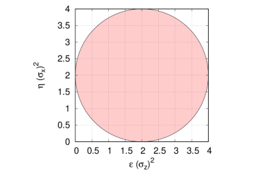
Figure 1: $\varepsilon(\sigma_{z})^{2}$ ​-​ $\eta(\sigma_{x})^{2}$ plot of tight EDR (18) for spin measurements in the state satisfying Eq. (22).

Lund and Wiseman Lund and Wiseman (2010) proposed a measurement model measuring the Pauli $\sigma_{z}=|0\rangle\langle 0|-|1\rangle\langle 1|$ observable of an abstract qubit described by the Hilbert space $\mathcal{H}=\mathbb{C}^{2}$ with a computational basis $\{|0\rangle,|1\rangle\}$. The probe is another qubit prepared in the state $|\xi(\theta)\rangle=\cos\theta|0\rangle+\sin\theta|1\rangle$ and the meter observable $M$ is chosen as the Pauli $\sigma_{z}$ observable of the probe. The measuring interaction is described by the unitary operator $U_{\text{CNOT}}$ on $\mathbb{C}^{2}\otimes\mathbb{C}^{2}$ performing the controlled-NOT operation controlled on the measured qubit. Thus, the measuring process is specified as ${\bf M}(\theta)=(\mathbb{C}^{2},|\xi(\theta)\rangle,U_{\text{CNOT}},\sigma_{z})$. Then, for the system state $|\psi\rangle=|\sigma_{y}=+1\rangle=(1/\sqrt{2})(|0\rangle+i|1\rangle)$, which satisfies condition (22) for $\rho=|\psi\rangle\langle\psi|$, the measurement error $\varepsilon(\sigma_{z})$ of ${\bf M}(\theta)$ for $A=\sigma_{z}$ and the disturbance $\eta(\sigma_{x})$ of ${\bf M}(\theta)$ for $B=\sigma_{x}$ is given by

$$\varepsilon(\sigma_{z}) =2|\sin\theta|,$$ (24)

$$\eta(\sigma_{x}) =\sqrt{2}|\cos\theta-\sin\theta|.$$ (25)

Thus, the error $\varepsilon(\sigma_{z})$ and disturbance $\eta(\sigma_{x})$ satisfy the relation

$$\left[\varepsilon(\sigma_{z})^{2}-2\right]^{2}+\left[\eta(\sigma_{x})^{2}-2\right]^{2}=4,$$ (26)

and attain the bound for the EDR (18). Experimental realizations of this EDR for optical polarization measurements were reported by Rozema et al. Rozema et al. (2012) and others Baek et al. (2013); Ringbauer et al. (2014); Kaneda et al. (2014).

In this paper we consider another type of measurement model, known as Stern-Gerlach measurements, measuring the $z$ component of the spin of a spin-1/2 particle, and investigate the admissible region of the error and disturbance obtained from Gaussian orbital states.

II.2 Stern-Gerlach measurements

Let us consider a measurement of the spin component of an electrically neutral spin-1/2 particle with a Stern-Gerlach apparatus. A particle moving along the $y$ axis passes through an inhomogeneous magnetic field and then the orbit is deflected, depending on the spin component of the particle along the direction of the magnetic field. This situation is illustrated in Fig. 2.

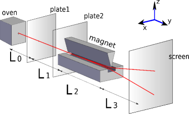
Figure 2: Illustration of the experimental setup for a Stern-Gerlach measurement. The relations between the length and the time interval are $L_{2}=v_{y}\Delta t$ and $L_{3}=v_{y}\tau$.

To analyze this measurement, we make the following assumptions.

• The magnetic field points everywhere on the $z$ axis.

• The strength of the magnetic field increases proportional to the $z$-coordinate,

  $$B_{z}=B_{0}+B_{1}z,$$ (27)

  where $B_{0}$ and $B_{1}$ are real numbers representing the value at the origin and the gradient of $B_{z}$, respectively.

• The velocity, $v_{y}$, in the $y$-direction is large in comparison with the motion in the $x$-$z$ plane and the length $L_{2}$ is large in comparison with the separation of the pole faces. Thus we can treat the times $\Delta t=L_{2}/v_{y}$ and $\tau=L_{3}/v_{y}$ as deterministic for our purpose, because the determination of the spin does not depend in a sensible way on the precise evaluation of $\Delta t$ and $\tau$ (see Bohm (1951), pp. 595-596).

To describe the measuring process $\mathbf{M}$ of a Stern-Gerlach measurement, the measured system $\mathbf{S}$ is taken as the spin degree of freedom described by the two-dimensional state space $\mathcal{H}$ with the Pauli operators $\sigma_{x}$, $\sigma_{y}$, and $\sigma_{z}$ describing the $x$, $y$, and $z$ components of the spin, respectively, of the spin-1/2 particle. The probe system $\mathbf{P}$ is taken as the orbital degree of freedom in the $z$ direction described by the Hilbert space, $\mathcal{K}$, of wave functions with position $Z$ and momentum $P$ satisfying the canonical commutation relation

$$[Z,P]=i\hbar.$$ (28)

The particle enters the magnetic field at time 0, emerges out of the magnetic field at time $\Delta t$, and freely evolves until time $\Delta t+\tau$ at which the particle reaches the screen and the observer can measure the meter observable $M$ that assigns $+1$ or $-1$ depending on the particle $z$ coordinate, $Z$, as $M=f(Z)$, with the function $f$ such that

$$f(z)=\begin{cases}-1&\mbox{if $z\geq 0$}\\ +1&\mbox{otherwise}.\end{cases}$$ (29)

Thus, the measuring process starts at time 0, when the system $\mathbf{S}$ is in any input state $\rho$ and the probe $\mathbf{P}$ is prepared in the fixed state $|\xi\rangle$, and ends up at time $t_{0}=\Delta t+\tau$. The time evolution operator $U=U(\Delta t+\tau)$ of the composite system $\mathbf{S}+\mathbf{P}$ during the measurement is determined by the time-dependent Hamiltonian $H(t)$ of the particle given by

$$H(t)\!=\!\left\{\begin{array}[]{lr}\mu\sigma_{z}\otimes\left(B_{0}+B_{1}Z\right)+\displaystyle\frac{1}{2m}\mathchoice{\rm 1\mskip-4.2mul}{\rm 1\mskip-4.2mul}{\rm 1\mskip-4.6mul}{\rm 1\mskip-5.2mul}\otimes P^{2},&0\leq t\leq\Delta t\\ \displaystyle\frac{1}{2m}\mathchoice{\rm 1\mskip-4.2mul}{\rm 1\mskip-4.2mul}{\rm 1\mskip-4.6mul}{\rm 1\mskip-5.2mul}\otimes P^{2},&\Delta t\leq t\leq\Delta t+\tau,\end{array}\right.$$ (30)

where $\mu$ denotes the magnetic moment of the particle and $m$ denotes the mass of the particle. By solving the Schrödinger equation, we obtain the time evolution operator $U(t)$ of $\mathbf{S}+\mathbf{P}$ for $0\leq t\leq\Delta t+\tau$ by

$$U(t)=\left\{\begin{array}[]{lr}\exp\left\{\displaystyle\frac{t}{i\hbar}\left[\mu\sigma_{z}\otimes\left(B_{0}\!+\!B_{1}Z\right)+\displaystyle\frac{1}{2m}\mathchoice{\rm 1\mskip-4.2mul}{\rm 1\mskip-4.2mul}{\rm 1\mskip-4.6mul}{\rm 1\mskip-5.2mul}\otimes P^{2}\right]\right\},&0\leq t\leq\Delta t\\ \exp\left(\displaystyle\frac{t-\Delta t}{2i\hbar m}\mathchoice{\rm 1\mskip-4.2mul}{\rm 1\mskip-4.2mul}{\rm 1\mskip-4.6mul}{\rm 1\mskip-5.2mul}\otimes P^{2}\right)\exp\left\{\displaystyle\frac{\Delta t}{i\hbar}\left[\mu\sigma_{z}\!\otimes\!\left(B_{0}\!+\!B_{1}Z\right)+\displaystyle\frac{1}{2m}\mathchoice{\rm 1\mskip-4.2mul}{\rm 1\mskip-4.2mul}{\rm 1\mskip-4.6mul}{\rm 1\mskip-5.2mul}\otimes P^{2}\right]\right\},&\Delta t\leq t\leq\Delta t+\tau.\end{array}\right.$$ (33)

To describe the time evolution of the composite system $\mathbf{S}+\mathbf{P}$ in the Heisenberg picture, we introduce Heisenberg operators for $0\leq t\leq\Delta t+\tau$ as

$$Z(0)=\mathchoice{\rm 1\mskip-4.2mul}{\rm 1\mskip-4.2mul}{\rm 1\mskip-4.6mul}{\rm 1\mskip-5.2mul}\otimes Z, \quad Z(t)=U(t)^{\dagger}Z(0)U(t),$$ (34)

$$P(0)=\mathchoice{\rm 1\mskip-4.2mul}{\rm 1\mskip-4.2mul}{\rm 1\mskip-4.6mul}{\rm 1\mskip-5.2mul}\otimes P, \quad P(t)=U(t)^{\dagger}P(0)U(t),$$ (35)

$$\sigma_{j}(0)=\sigma_{j}\otimes\mathchoice{\rm 1\mskip-4.2mul}{\rm 1\mskip-4.2mul}{\rm 1\mskip-4.6mul}{\rm 1\mskip-5.2mul}, \quad\sigma_{j}(t)=U(t)^{\dagger}\sigma_{j}(0)U(t),$$ (36)

where $j=x,y,z$. For the relation between the time evolution operators in the Heisenberg picture and the Schrödinger picture, we refer the reader to Appendix D.

We also use the matrix representations of Pauli operators as

$$\sigma_{x}=\left(\begin{array}[]{cc}0&1\\ 1&0\end{array}\right), \quad\sigma_{y}=\left(\begin{array}[]{cc}0&-i\\ i&0\end{array}\right),\quad\sigma_{z}=\left(\begin{array}[]{cc}1&0\\ 0&-1\end{array}\right).$$ (43)

By solving Heisenberg equations of motion for $Z(t)$, $P(t)$, $\sigma_{x}(t)$, $\sigma_{y}(t)$, and $\sigma_{z}(t)$, as shown in Appendix E, we have

$$Z(\Delta t+\tau) =Z(0)+\frac{\Delta t+\tau}{m}P(0)$$

$$\quad-\frac{\mu B_{1}\Delta t}{m}\left(\tau+\frac{\Delta t}{2}\right)\sigma_{z}(0),$$ (44)

$$P(\Delta t+\tau) =P(0)-\mu B_{1}\Delta t\sigma_{z}(0),$$ (45)

$$\sigma_{x}(\Delta t+\tau) =\left(\begin{array}[]{cc}0&\exp\left[iS(\Delta t)\right]\\ \exp\left[-iS(\Delta t)\right]&0\end{array}\right),$$ (48)

$$\sigma_{y}(\Delta t+\tau) =\left(\begin{array}[]{cc}0&-i\exp\left[iS(\Delta t)\right]\\ i\exp\left[-iS(\Delta t)\right]&0\end{array}\right),$$ (51)

$$\sigma_{z}(\Delta t+\tau) =\sigma_{z}(0),$$ (52)

where

$$S(\Delta t) = \frac{2\mu\Delta t}{\hbar}\left[B_{0}+B_{1}\left(Z(0)+\frac{\Delta t}{2m}P(0)\right)\right].$$ (53)

III Error

Let us consider the quantum rms error of a Stern-Gerlach measurement $\mathbf{M}$ of the $z$ component $\sigma_{z}(0)$ of the spin at time 0 using the meter observable

$$M(\Delta t+\tau)=f(Z(\Delta t+\tau)),$$ (54)

introduced in Sec. II. The noise operator $N$ of this measurement is given by

$$N=M(\Delta t+\tau)-\sigma_{z}(0).$$ (55)

The initial state $\rho$ of the spin $\mathbf{S}$ is supposed to be an arbitrary state with the matrix

$$\rho=\frac{1}{2}(\mathchoice{\rm 1\mskip-4.2mul}{\rm 1\mskip-4.2mul}{\rm 1\mskip-4.6mul}{\rm 1\mskip-5.2mul}+n_{x}\sigma_{x}+n_{y}\sigma_{y}+n_{z}\sigma_{z})$$ (56)

where $n_{x},n_{y},n_{z}\in\mathbb{R}$ and $n_{x}^{2}+n_{y}^{2}+n_{z}^{2}\leq 1$, so that the initial state of the composite system $\mathbf{S}+\mathbf{P}$ is given by $\rho\otimes\left|\xi\right\rangle\left\langle\xi\right|$, where $|\xi\rangle$ is a fixed but arbitrary wave function describing the initial state of the orbital degree of freedom $\mathbf{P}$. Then the error, namely, the quantum rms error, of this measurement of $\sigma_{z}$ is given by

$$\varepsilon(\sigma_{z})=\sqrt{\langle N^{2}\rangle_{\rho\otimes\left|\xi\right\rangle\left\langle\xi\right|}},$$ (57)

where we abbreviate $\mathrm{Tr}(A\rho)$ as $\langle A\rangle_{\rho}$ for observable $A$ and density operator $\rho$. We will give an explicit formula for $\varepsilon(\sigma_{z})$, which eventually shows that the error depends only on the parameter $n_{z}$ in Eq. (56).

Let

$$U_{t} =\exp\left[\frac{t}{2i\hbar m}P^{2}\right],$$ (58)

$$\tilde{U}_{t} =\mathchoice{\rm 1\mskip-4.2mul}{\rm 1\mskip-4.2mul}{\rm 1\mskip-4.6mul}{\rm 1\mskip-5.2mul}_{\mathbf{S}}\otimes U_{t},$$ (59)

$$g_{0} =\frac{\mu B_{1}\Delta t}{m}\left(\tau+\frac{\Delta t}{2}\right).$$ (60)

From Eq. (44) we have

$$Z(\Delta t+\tau)$$

$$=\tilde{U}_{\Delta t+\tau}^{{\dagger}}\left(\begin{array}[]{cc}Z-g_{0}&0\\ 0&Z+g_{0}\end{array}\right)\tilde{U}_{\Delta t+\tau}.$$ (63)

Thus, we have

$$N =f(Z(\Delta t+\tau))-\sigma_{z}(0)$$

$$=2\tilde{U}_{\Delta t+\tau}^{{\dagger}}\left(\begin{array}[]{cc}-\chi_{+}(Z-g_{0})&0\\ 0&\chi_{-}(Z+g_{0})\\ \end{array}\right)\tilde{U}_{\Delta t+\tau},$$ (66)

where

$$\chi_{+}(z) =\begin{cases}1&\mbox{if $z\geq 0$},\\ 0&\mbox{otherwise},\end{cases}$$ (67)

$$\chi_{-}(z) =1-\chi_{+}(z),$$ (68)

$$f(z) =1-2\chi_{+}(z).$$ (69)

It follows that

$$N^{2} =4\tilde{U}_{\Delta t+\tau}^{{\dagger}}\left(\begin{array}[]{cc}\chi_{+}(Z-g_{0})&0\\ 0&\chi_{-}(Z+g_{0})\\ \end{array}\right)\tilde{U}_{\Delta t+\tau}.$$ (72)

Therefore, we have

$$\varepsilon(\sigma_{z})^{2} =\langle N^{2}\rangle_{\rho\otimes\left|\xi\right\rangle\left\langle\xi\right|}$$

$$=\left\langle\xi|\mbox{\rm Tr}_{\mathbf{S}}[N^{2}\rho]|\xi\right\rangle$$

$$=2(1+n_{z})\langle\xi|U_{\Delta t+\tau}^{{\dagger}}\chi_{+}(Z-g_{0})U_{\Delta t+\tau}^{{\dagger}}|\xi\rangle$$

$$\quad+2(1-n_{z})\langle\xi|U_{\Delta t+\tau}^{{\dagger}}\chi_{-}(Z-g_{0})U_{\Delta t+\tau}^{{\dagger}}|\xi\rangle.$$ (73)

Consequently, we have

$$\varepsilon(\sigma_{z})^{2} =2(1+n_{z})\int_{g_{0}}^{\infty}|U_{\Delta t+\tau}\xi(z)|^{2}dz\biggr{.}$$

. $$\qquad\qquad\qquad+2(1-n_{z})\int_{-\infty}^{-g_{0}}|U_{\Delta t+\tau}\xi(z)|^{2}dz.\biggr{.}$$ (74)

IV Disturbance

Let us consider the quantum rms disturbance, $\eta(\sigma_{x})$, for the $x$-component of the spin in Stern-Gerlach measurements. The disturbance operator, $\sigma_{x}$, is given by

$$D=\sigma_{x}(\Delta t+\tau)-\sigma_{x}(0).$$ (75)

From Eq. (48) we have

$$D=\left(\begin{array}[]{cc}0&\exp\left[iS(\Delta t)\right]-1\\ \exp\left[-iS(\Delta t)\right]-1&0\end{array}\right).$$ (76)

Consequently, we have

$$D^{2}=\mathchoice{\rm 1\mskip-4.2mul}{\rm 1\mskip-4.2mul}{\rm 1\mskip-4.6mul}{\rm 1\mskip-5.2mul}\otimes\left[2-2\cos S(\Delta t)\right],$$ (77)

and thus

$$\eta(\sigma_{x})^{2}$$

$$=2\!-\!2\left\langle\cos\!\left\{\!\frac{2\mu\Delta t}{\hbar}\left[\!B_{0}+B_{1}\left(\!Z+\frac{\Delta t}{2m}P\right)\!\right]\!\right\}\right\rangle_{\xi}.$$ (78)

V Error and disturbance for Gaussian states

Let us consider the error and disturbance in Stern-Gerlach measurements under the condition that the orbital state of the particle is in the family $\mathcal{G}$ of Gaussian states given by

$$\mathcal{G}=\left\{\xi_{\lambda}\in\mathit{L}^{2}(\mathbb{R})\mathrel{}\left|\mathrel{}\begin{array}[]{l}\xi_{\lambda}(z)=A\exp(-\lambda z^{2})\\[5.0pt] \displaystyle\int_{-\infty}^{\infty}|\xi_{\lambda}(z)|^{2}dz=1\\[10.00002pt] \lambda\in\mathbb{C},{\rm Re\,}(\lambda)>0\end{array}\right.\right\}.$$ (79)

This family of states consists of all Gaussian pure states Schumaker (1986), whose mean values of the position and momentum are both $0$. For simplicity, it is assumed that the spin state of the particle is in the eigenstate of the spin component $\sigma_{y}$. It is easy to minimize the error of the measurement with respect to the mean values of the position and momentum. In particular, $\mathcal{G}$ is the family of optimal states for the measurement among the Gaussian pure states if the spin state of the particle is the eigenstate of $\sigma_{y}$. We remark that the equality in the Schrödinger inequality [see Eq. (138) ] holds for any state $\xi$ in $\mathcal{G}$, i.e.,

$$\langle Z^{2}\rangle_{\xi}\langle P^{2}\rangle_{\xi}-\frac{1}{4}\langle\{Z,P\}\rangle_{\xi}^{2}=\frac{\hbar^{2}}{4}.$$ (80)

Here we use the abbreviation $\langle A\rangle_{\xi}=\langle\xi|A|\xi\rangle$. The converse also holds, that is, any state $\xi$ satisfying $\langle P\rangle_{\xi}=\langle Z\rangle_{\xi}=0$ and Eq. (80) belongs to $\mathcal{G}$.

Let us consider the range of the error and disturbance of Stern-Gerlach measurements. Let

$$V(\psi,t) =\left\langle\left(Z+\frac{t}{m}P\right)^{2}\right\rangle_{\psi}$$ (81)

for any orbital state $\psi$. For the disturbance $\eta(\sigma_{x})$, from Eq. (78) we have

$$\eta(\sigma_{x})^{2}$$

$$=2-2\left\langle\cos\left[\frac{2\mu\Delta t}{\hbar}\left(B_{0}+B_{1}Z\right)\right]\right\rangle_{U_{\Delta t/2}\xi_{\lambda}}$$

$$=2-\frac{2}{\sqrt{2\pi V(\xi_{\lambda},\Delta t/2)}}$$

$$\times \int_{-\infty}^{\infty}\exp\left(-\frac{z^{2}}{2V(\xi_{\lambda},\Delta t/2)}\right)\cos\left[\frac{2\mu\Delta t}{\hbar}\left(B_{0}+B_{1}z\right)\right]dz$$

$$=2-2\exp\!\left(-\frac{2\mu^{2}\!B_{1}^{2}\!\Delta t^{2}}{\hbar^{2}}V(\xi_{\lambda},\Delta t/2)\right)\cos\frac{2\mu\Delta tB_{0}}{\hbar}.$$ (82)

From the above formula, the disturbance is determined by $V(\xi_{\lambda},\Delta t/2)$ and the parameters of the magnet if the orbital state is in $\mathcal{G}$. Now, for a fixed constant $v$ let us find the error for state $\xi_{\lambda}$ in $\mathcal{G}$ and time interval $\Delta t$ satisfying $V(\xi_{\lambda},\Delta t/2)=v$. In the following, we fix the time interval $\Delta t$.

From Eq. (74) we have

$$\varepsilon(\sigma_{z})^{2} = 4\int_{g_{0}}^{\infty}\left|U_{\Delta t+\tau}\xi_{\lambda}(z)\right|^{2}dz$$ (83)

$$= \frac{4}{\sqrt{\pi}}\int_{{g_{0}}/{\sqrt{2V(\xi_{\lambda},\Delta t+\tau)}}}^{\infty}\exp(-w^{2})dw.$$

Here we use the relation $n_{z}=0$, which is obtained from the assumption that the mean value of the $z$ component of the spin of the particle is $0$. Equation (83) shows that the error is minimized by maximizing the lower limit of the integration $g_{0}/\sqrt{2V(\xi_{\lambda},\Delta t+\tau)}$. First, we fix the state $\xi_{\lambda}$ and focus on the time interval $\tau$. Let $W_{\xi_{\lambda}}(\tau)=g_{0}/\sqrt{2V(\xi_{\lambda},\Delta t+\tau)}$. From now on, we suppose $B_{1}\leq 0$. As shown in Appendix F, if

$$m\left\langle\left\{Z,P\right\}\right\rangle_{\xi_{\lambda}}+\left\langle P^{2}\right\rangle_{\xi_{\lambda}}\Delta t<0$$ (84)

holds, then $W_{\xi_{\lambda}}(\tau)$ assumes the maximum value

$$W_{\xi_{\lambda}}(\tau_{0})=\frac{\sqrt{2V(\xi_{\lambda},\Delta t/2)}\mu B_{1}\Delta t}{\hbar}$$ (85)

at

$$\tau= \tau_{0}$$

$$= -\frac{4m^{2}\left\langle Z^{2}\right\rangle_{\xi_{\lambda}}+3m\left\langle\left\{Z,P\right\}\right\rangle_{\xi_{\lambda}}\Delta t+2\left\langle P^{2}\right\rangle_{\xi_{\lambda}}\Delta t^{2}}{2\left(m\left\langle\left\{Z,P\right\}\right\rangle_{\xi_{\lambda}}+\left\langle P^{2}\right\rangle_{\xi_{\lambda}}\Delta t\right)}.$$ (86)

On the other hand, if condition (84) does not hold, the supremum of $W_{\xi_{\lambda}}(\tau)$ is given by

$$\sup_{\tau\geq 0}W_{\xi_{\lambda}}(\tau)=\lim_{\tau\to\infty}W_{\xi_{\lambda}}(\tau)=\frac{\mu B_{1}\Delta t}{\sqrt{2}}\left\langle P^{2}\right\rangle_{\xi_{\lambda}}^{-1/2}.$$ (87)

Now let us consider the maximization of $W_{\xi_{\lambda}}(\tau)$ with respect to the state $\xi_{\lambda}$. For any pair of orbital states $\psi$ and $\phi$ in $\mathcal{G}$ satisfying $V(\psi,\Delta t/2)=v$ and $V(\phi,\Delta t/2)=v$, respectively, if $\psi$ satisfies condition (84), then

$$W_{\psi}(\tau_{0})\geq\lim_{\tau\to\infty}W_{\phi}(\tau)$$ (88)

holds, since $W_{\psi}(\tau_{0})/\lim_{\tau\to\infty}W_{\phi}(\tau)\geq 1$ by the Kennard inequality (2). Therefore, we obtain the supremum of $W_{\xi_{\lambda}}(\tau)$ with respect to the state $\xi_{\lambda}$ and time interval $\tau$ as

$$\sup_{\mathrm{Re}(\lambda)>0,\tau\geq 0}W_{\xi_{\lambda}}(\tau)=\frac{\sqrt{2v}\mu B_{1}\Delta t}{\hbar}.$$ (89)

See Appendix F for the detailed derivation.

Although the above argument is for finding the range of the error and disturbance that Stern-Gerlach measurements can assume, it contains one more important assertion. That is, the calculation suggests that the error of Stern-Gerlach measurements is minimized by placing the screen at a finite distance from the magnet under the condition represented by (84), in contrast to the conventional assumption that the error is minimized by placing the screen at infinity. If a state in $\mathcal{G}$ satisfies condition (84), then the correlation term Yuen (1983) $\left\langle\left\{Z-\left\langle Z\right\rangle_{\xi_{\lambda}},P-\left\langle P\right\rangle_{\xi_{\lambda}}\right\}\right\rangle_{\xi_{\lambda}}$ is negative, and this leads to a narrowing of the standard deviation of the position of the particle during the free evolution (see Appendix B.4). Such a class of states was introduced by Yuen Yuen (1983) and they are known as contractive states.

Let us return to the problem of finding the range of values of the error and disturbance that Stern-Gerlach measurements can assume. Now setting $W_{0}={\sqrt{2v}\mu B_{1}\Delta t}/{\hbar}$, the disturbance and the infimum of the error under the condition that $V(\lambda,\Delta t/2)=v$ for fixed $\Delta t$ and $v$ are

$$\eta(\sigma_{x})^{2} = 2-2\exp\left(-W_{0}^{2}\right)\cos\frac{2\mu\Delta tB_{0}}{\hbar},$$ (90)

$$\inf_{\lambda,T}\varepsilon(\sigma_{z})^{2} = \frac{4}{\sqrt{\pi}}\int_{W_{0}}^{\infty}\exp(-w^{2})dw,$$ (91)

respectively. By varying the parameter of the magnet $B_{0}$, we obtain the range of the disturbance as

$$2-2\exp\left(-W_{0}^{2}\right)\leq\eta(\sigma_{x})^{2}\leq 2+2\exp\left(-W_{0}^{2}\right).$$ (92)

We obtain the range of the disturbance and the infimum of the error of Stern-Gerlach measurements for each constant $v$. By varying $v$, we obtain the range of the error and disturbance as the inequalities

$$\left|\frac{\eta(\sigma_{x})^{2}-2}{2}\right|\leq\exp\left\{-\left[\mathrm{erf}^{-1}\left(\frac{\varepsilon(\sigma_{z})^{2}-2}{2}\right)\right]^{2}\right\},$$ (93)

$$0\leq\varepsilon(\sigma_{z})^{2}\leq 2,$$ (94)

where $\mathrm{erf}^{-1}$ represents the inverse of the error function $\mathrm{erf}(x)=({2}/{\sqrt{\pi}})\int_{0}^{x}\exp(-s^{2})ds$. The square of the error varies from $0$ to $2$ since $W_{0}$ is positive.

We now remove the constraint $B_{1}\leq 0$. For $B_{1}\geq 0$, similarly to the above discussion, we have

$$\left|\frac{\eta(\sigma_{x})^{2}-2}{2}\right|\leq\exp\left\{-\left[\mathrm{erf}^{-1}\left(\frac{\varepsilon(\sigma_{z})^{2}-2}{2}\right)\right]^{2}\right\},$$ (95)

$$2\leq\varepsilon(\sigma_{z})^{2}\leq 4.$$ (96)

Therefore, we have

$$\left|\frac{\eta(\sigma_{x})^{2}-2}{2}\right|\leq\exp\left\{-\left[\mathrm{erf}^{-1}\left(\frac{\varepsilon(\sigma_{z})^{2}-2}{2}\right)\right]^{2}\right\}.$$ (97)

The plot of this region is shown in Fig. 3.

For comparison, the figure shows the plot of the boundary of the Branciard-Ozawa tight EDR (23) for general spin measurement. From this plot, we conclude that the range of the error and disturbance for Stern-Gerlach measurements considered in this paper is close to the theoretical optimal given by the Branciard-Ozawa tight EDR (23). Here the range of the error and disturbance for Stern-Gerlach measurements is also compared with Heisenberg’s EDR (6) (green line) and the EDR (7) for the neutron experiment Erhart et al. (2012); Sulyok et al. (2013) (black line). We conclude that Stern-Gerlach measurements actually violate Heisenberg’s EDR (6) in a broad range of experimental parameters.

Roughly speaking, the parameter $v$ represents the spread of the wave packet of the particle in the Stern–Gerlach magnet. The reason why $v$ appears in the formula of the disturbance is that the particle in the Stern-Gerlach magnet is exposed to the inhomogeneous magnetic field and its spin is precessed in an uncontrollable way. This uncontrollable precession occurs because the position of the particle is uncertain while the magnetic field is inhomogeneous and hence depends on the position. The disturbance of the spin along the $x$ axis is caused by this uncontrollable precession around the $z$ axis. This is why $v$ appears in the formula of the disturbance. On the other hand, the error in our Stern-Gerlach setup comes from the non zero dispersion of the $z$ component of the particle position when the particle has reached the screen. The smaller the dispersion of the particle position when the particle has reached the screen, the greater the dispersion of the $z$ component of the particle position in the Stern-Gerlach magnet. This is why $v$ appears in the formula of the error.

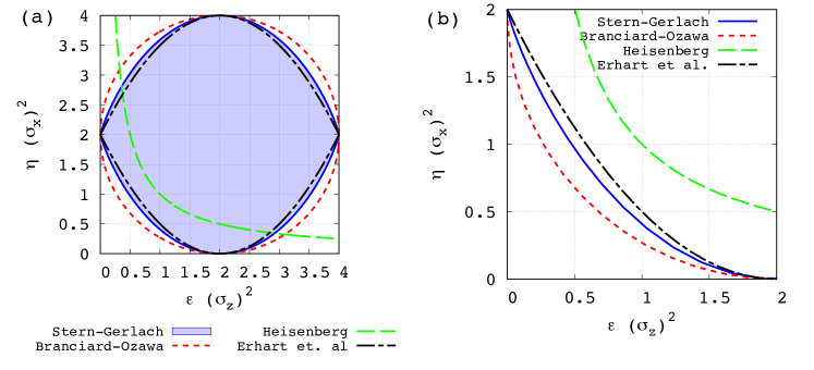
Figure 3: (a) Range of error and disturbance for Stern-Gerlach measurements. The blue region is the region (97) that Stern-Gerlach measurements can achieve. The red dotted line is the boundary of the Branciard-Ozawa tight EDR (23). The green dashed line is the boundary of Heisenberg’s EDR (6). The black dash-dotted line is the theoretical boundary (7) of the EDR of the experiment conducted by Erhart and co-workers Erhart et al. (2012); Sulyok et al. (2013). The error-disturbance region of Stern-Gerlach measurements is close to the theoretical optimum given by the Branciard-Ozawa tight EDR (23) and actually violates Heisenberg’s EDR (6) in a broad range of experimental parameters. (b) Enlarged plot for the part $[0,2]\times[0,2]$.

VI Comparison with “aspects of nonideal Stern-Gerlach experiment and testable ramifications”

Home et al. Home et al. (2007) discussed the same error of Stern-Gerlach measurements as our paper does for similar conditions. We consider in what sense their paper is related to ours and we compare its results with ours. They derived the wave function of a particle in the Stern-Gerlach apparatus under the following conditions.

• The magnetic field is oriented along the $z$ axis everywhere and the gradient of the $z$ component of the magnetic field is non zero only in the $z$ direction.

• The initial orbital state is a Gaussian state whose mean values of the position and momentum, and the correlation term of the particle in the wave function are all zero.

• Unlike Bohm’s discussion Bohm (1951), the kinetic energy of the particle in the magnetic field is not neglected.

Based on their argument, they discussed the distinguishability of the value of the measured observable by observing the probe system directly in Stern-Gerlach measurements. To consider this problem, they introduced the two indices,

$$I:=\left|\int_{-\infty}^{\infty}\int_{-\infty}^{\infty}\int_{-\infty}^{\infty}\psi_{+}^{*}(\mathbf{x},\tau)\psi_{-}(\mathbf{x},\tau)d\mathbf{x}\right|,$$ (98)

$$E(t):=\int_{-\infty}^{0}\int_{-\infty}^{\infty}\int_{-\infty}^{\infty}\left|\psi_{+}(\mathbf{x},t)\right|^{2}dxdydz,$$ (99)

where $\psi_{\pm}$ are the wave functions of the particle in the Schrödinger picture whose spin $z$ components are $\pm 1/2$, respectively. The origin of time is taken to be the moment when the particle enters the Stern-Gerlach magnet. In addition, $\tau$ is the time at which the particle emerges from the Stern-Gerlach magnet ($\tau$ corresponds to $\Delta t$ in our notation) and $t$ is any time after emerging from the Stern-Gerlach magnet ($t$ corresponds to $\Delta t+\tau$ in our notation). Namely, they adopted the inner product $I$ of the two wave functions with different spin directions, and the probability $E(t)$ of finding the particle with the spin $z$ components of $+1/2$ and $-1/2$ within the lower and upper half planes, respectively, at time $t$. They concluded that $I$ always vanishes whenever $E(t)$ vanishes, but that $E(t)$ does not necessarily vanish even when $I$ vanishes.

We discuss the relation between their paper and ours. The relation between the quantities $E(t)$ and $\varepsilon(\sigma_{z})$ is

$$\varepsilon(\sigma_{z})^{2}=4E(t).$$ (100)

Although this relation is model dependent, it bridges the two approaches and will enforce a theoretical background for our definition of a sound and complete quantum generalization of the classical root-mean-square error Ozawa (2019).

We compare their research with ours as follows.

• Their setup and approximation are the same as ours and they used the same Hamiltonian as in our research.

• In both papers, the orbital state of the particle is assumed to be the pure state where the mean values of its position and momentum are zero. We assume that the correlation term of a Gaussian pure state is not necessarily zero, whereas they assumed that the orbital state is a Gaussian pure state with no correlation.

• We evaluate the tradeoff between the error and disturbance, whereas they compared the error with the inner product $I$ of the emerging wave functions expressing formal distinguishability. In addition, we obtain the range of error and disturbance under the condition that the orbital state is a Gaussian pure state whose correlation term is not necessarily zero.

VII Conclusion

Stern-Gerlach measurements, originally performed by Gerlach and Stern Gerlach and Stern (1922a, b, c), have been discussed for a long time as a typical model or a paradigm of quantum measurement Bohm (1951). As Heisenberg’s uncertainty principle suggests, Stern-Gerlach measurements of one spin component inevitably disturb its orthogonal component, and Heisenberg’s EDR (6) has been commonly believed to be its precise quantitative expression. However, general quantitative relations between error and disturbance in arbitrary quantum measurements have been extensively investigated over the past two decades and universally valid EDRs have been obtained to reform Heisenberg’s original EDR (see, e.g., Ozawa (2003a); Erhart et al. (2012); Branciard (2013); Busch et al. (2014); Ozawa (2019) and references therein).

Here we investigated the EDR for this familiar class of measurements in light of the general theory leading to the universally valid EDR relations. We have determined the range of possible values of the error and disturbance achievable by arbitrary Stern-Gerlach apparatuses, assuming that the orbital state is a Gaussian state. Our result is depicted in Fig. 3 and the boundary of the error-disturbance region is given in Eq. (97) as a closed formula. The result shows that the error-disturbance region of Stern-Gerlach measurements occupies a near-optimal subregion of the universally valid error-disturbance region for arbitrary measurements. It can be seen that one of the earliest methods of quantum measurement violates Heisenberg’s EDR (6) in a broad range of experimental parameters. Furthermore, we found a class of initial orbital states in which the error can be minimized an arbitrarily small amount by the screen at a finite distance from the magnet in contrast to the conventional assumption that the error decreases asymptotically.

The relation for the general class of states beyond Gaussian states is left to future study. In addition, we also leave it to future research to analyze more realistic models, for example, a model described by the magnetic field satisfying Maxwell’s equations Cruz-Barrios and Gómez-Camacho (2000); Potel et al. (2005) or a model considering the decoherence of the particle during the measuring process Devereux (2015).

Our results will contribute to answer the question as to how various experimental parameters can be controlled to achieve the ultimate limit. We expect that the present study will provoke further experimental studies.

Appendix A Error and disturbance in quantum measurements

In this appendix, we review the general theory of error and disturbance in quantum measurements developed in Ozawa (2004, 2019).

A.1 Classical root-mean-square error

Let us consider the classical case first. Recall the root-mean-square (rms) error introduced by Gauss Gauss (1995). Consider a measurement of the value $x$ of a quantity $X$ by actually observing the value $y$ of a meter quantity $Y$. Then the error of this measurement is given by $y-x$. If these quantities obey a joint probability distribution $\mu(x,y)$, then the rms error $\varepsilon_{G}(\mu)$ is defined as

$$\varepsilon_{G}(\mu)=\left(\sum_{x,y}(y-x)^{2}\,\mu(x,y)\right)^{1/2}.$$ (101)

A.2 Quantum measuring processes

We consider a quantum system $\mathbf{S}$ described by a finite-dimensional Hilbert space $\mathcal{H}$. We assume that every measuring apparatus for the system $\mathbf{S}$ has its own output variable $\mathbf{x}$. The statistical properties of the apparatus $\mathbf{A}(\mathbf{x})$ having the output variable $\mathbf{x}$ are determined by (i) the probability distribution $\Pr\{\mathbf{x}=m\|\rho\}$ of $\mathbf{x}$ for the input state $\rho$, and (ii) the output state $\rho_{\{\mathbf{x}=m\}}$ given the outcome $\mathbf{x}=m$.

A measuring process of the apparatus $\mathbf{A}(\mathbf{x})$ measuring $\mathbf{S}$ is specified by a quadruple $\mathbf{M}=(\mathcal{K},|\xi\rangle,U,M)$ consisting of a Hilbert space $\mathcal{K}$ describing the probe system $\mathbf{P}$, a state vector $|\xi\rangle$ in $\mathcal{K}$ describing the initial state of $\mathbf{P}$, a unitary operator $U$ on $\mathcal{H}\otimes\mathcal{K}$ describing the time evolution of the composite system $\mathbf{S}+\mathbf{P}$ during the measuring interaction, and an observable, $M$, called the meter observable, of $\mathbf{P}$ describing the meter of the apparatus.

The instrument of the measuring process $\mathbf{M}$ is defined as a completely positive map valued function $\mathcal{I}$ given by

$$\mathcal{I}(m)\rho=\mbox{\rm Tr}_{\mathcal{K}}[(\mathchoice{\rm 1\mskip-4.2mul}{\rm 1\mskip-4.2mul}{\rm 1\mskip-4.6mul}{\rm 1\mskip-5.2mul}\otimes P^{M}(m))U(\rho\otimes|\xi\rangle\langle\xi|)U^{\dagger}]$$ (102)

for any state $\rho$ and real number $m$. The statistical properties of the apparatus $\mathbf{A}(\mathbf{x})$ are determined by the instrument $\mathcal{I}$ of $\mathbf{M}$ as

$$\Pr\{\mathbf{x}=m\|\rho\} =\mbox{\rm Tr}[\mathcal{I}(m)\rho],$$ (103)

$$\rho_{\{\mathbf{x}=m\}} =\frac{\mathcal{I}(m)\rho}{\mbox{\rm Tr}[\mathcal{I}(m)\rho]}.$$ (104)

The non-selective operation $T$ of $\mathbf{M}$ is defined by

$$T=\sum_{m\in\mathbb{R}}\mathcal{I}(m).$$ (105)

Then we have

$$T(\rho)=\mbox{\rm Tr}_{\mathcal{K}}[U(\rho\otimes|\xi\rangle\langle\xi|)U^{\dagger}].$$ (106)

See Refs. Ozawa (1984, 1989, 2004) for detailed descriptions of measuring processes and instruments.

A.3 Heisenberg picture

In the measuring process $\mathbf{M}$, we suppose that the measuring interaction is turned on from time $t=0$ to time $t=t_{0}$. Then, the outcome $\mathbf{x}=m$ of the apparatus $\mathbf{A}(\mathbf{x})$ described by the measuring process $\mathbf{M}$ is defined as the outcome $m$ of the meter measurement at time $t=t_{0}$. To describe the time evolution of the composite system $\mathbf{S}+\mathbf{P}$ in the Heisenberg picture, let

$$\begin{array}[]{rclcrclc}A(0)&=&A\otimes\mathchoice{\rm 1\mskip-4.2mul}{\rm 1\mskip-4.2mul}{\rm 1\mskip-4.6mul}{\rm 1\mskip-5.2mul},&&A(t_{0})&=&U^{\dagger}A(0)U,\\ B(0)&=&B\otimes\mathchoice{\rm 1\mskip-4.2mul}{\rm 1\mskip-4.2mul}{\rm 1\mskip-4.6mul}{\rm 1\mskip-5.2mul},&&B(t_{0})&=&U^{\dagger}B(0)U,\\ M(0)&=&\mathchoice{\rm 1\mskip-4.2mul}{\rm 1\mskip-4.2mul}{\rm 1\mskip-4.6mul}{\rm 1\mskip-5.2mul}\otimes M,&&M(t_{0})&=&U^{\dagger}M(0)U,\end{array}$$ (110)

where $A$ and $B$ are observables of $\mathbf{S}$.

Then, the POVM $\Pi$ of $\mathbf{M}$ is defined as

$$\Pi(m)=\langle\xi|P^{M(t_{0})}(m)|\xi\rangle$$ (111)

and satisfies

$$\Pr\{\mathbf{x}=m\|\rho\}=\mbox{\rm Tr}[\Pi(m)\rho].$$ (112)

The $n$-th moment operator of $\Pi$ for $n=1,\ldots,n$ is defined by

$$\hat{\Pi}^{(n)}=\left\langle\xi\left|M(t_{0})^{n}\right|\xi\right\rangle.$$ (113)

The dual non-selective operation $T^{*}$ of $\mathbf{M}$ is defined by

$$T^{*}(B)=\langle\xi|B(t_{0})|\xi\rangle$$ (114)

for any observable $B$ of $\mathbf{S}$ and satisfies

$$\mbox{\rm Tr}\left\{\left[T^{*}(B)\right]\rho\right\}=\mbox{\rm Tr}\left\{B\left[T(\rho)\right]\right\}$$ (115)

for any observable $B$ and state $\rho$.

A.4 Measurement of observables

If the observables $A(0)$ and $M(t_{0})$ commute in the initial state $\rho\otimes|\xi\rangle\langle\xi|$, that is,

$$[P^{A(0)}(a),P^{M(t_{0})}(m)](\rho\otimes\left|\xi\rangle\langle\xi\right|)=0$$ (116)

for all $a,m\in\mathbb{R}$, then their joint probability distribution $\mu(a,m)$ is defined as

$$\mu(a,m)=\mathrm{Tr}[P^{A(0)}(a)P^{M(t_{0})}(m)\,(\rho\otimes|\xi\rangle\langle\xi|)]$$ (117)

and satisfies

$$\mathrm{Tr}[f(A(0),M(t_{0}))(\rho\otimes|\xi\rangle\langle\xi|)]=\sum_{a,m}f(a,m)\,\mu(a,m)$$ (118)

for any polynomial $f(A(0),M(t_{0}))$ of $A(0)$ and $M(t_{0})$.

We say that the measuring process $\mathbf{M}$ accurately measures the observable $A$ in a state $\rho$ if $A(0)$ and $M(t_{0})$ are perfectly correlated in the state $\rho\otimes\left|\xi\rangle\langle\xi\right|$ Ozawa (2005, 2006a, 2019), namely, one of the following two equivalent conditions holds: (i) $A(0)$ and $M(t_{0})$ commute in $\rho\otimes|\xi\rangle\langle\xi|$ and their joint probability distribution $\mu$ satisfies

$$\sum_{a,m:a=m}\mu(a,m)=1$$ (119)

or (ii) for any $a,m\in\mathbb{R}$ with $a\neq m$,

$$\mathrm{Tr}\left[\Pi(m)P^{A}(a)\,\rho\right]=0.$$ (120)

Note that $\nu(a,m):=\mathrm{Tr}\left[\Pi(m)P^{A}(a)\,\rho\right]$, called the weak joint distribution of $A(0)$ and $M(t_{0})$, always exists and is operationally accessible by weak measurement and post-selection Jozsa (2007); Lund and Wiseman (2010), but possibly takes negative or complex values. Since $\nu(a,m)$ is operationally accessible, our definition of accurate measurements is operationally accessible.

A.5 Quantum root-mean-square error

The noise operator $N(A,\mathbf{M})$ of the measuring process $\mathbf{M}$ for measuring $A$ is defined as

$$N(A,\mathbf{M})=M(t_{0})-A(0).$$ (121)

The (noise-operator based) quantum rms error $\varepsilon_{{\rm NO}}(A,\mathbf{M},\rho)$ for measuring $A$ in $\rho$ by $\mathbf{M}$ is defined as the root mean square of the noise operator, i.e.,

$$\varepsilon_{{\rm NO}}(A,\mathbf{M},\rho)=\left\{\mathrm{Tr}\left[N(A,\mathbf{M})^{2}(\rho\otimes|\xi\rangle\langle\xi|)\right]\right\}^{1/2}.$$ (122)

To argue the reliability of the error measure $\varepsilon_{{\rm NO}}$ defined above, we consider the following requirements for any reliable error measures $\varepsilon$ generalizing the classical root-mean-square error $\varepsilon_{G}$ to quantify the mean error $\varepsilon(A,\mathbf{M},\rho)$ of the measurement of an observable $A$ in a state $\rho$ described by a measuring process $\mathbf{M}$ Ozawa (2019).

• Operational definability. The error measure $\varepsilon$ should be definable by the POVM $\Pi$ of the measuring process $\mathbf{M}$ with the observable $A$ to be measured and the initial state $\rho$ of the measured system $\mathbf{S}$.

• Correspondence principle. In the case where $A(0)$ and $M(t_{0})$ commute in $\rho\otimes|\xi\rangle\langle\xi|$, the relation

  $$\varepsilon(A,\mathbf{M},\rho)=\varepsilon_{G}(\mu)$$ (123)

  holds for the joint probability distribution $\mu$ of $A(0)$ and $M(t_{0})$ in $\rho\otimes|\xi\rangle\langle\xi|$.

• Soundness. If $\mathbf{M}$ accurately measures $A$ in $\rho$, then $\varepsilon$ vanishes, i.e., $\varepsilon(A,\mathbf{M},\rho)=0$.

• Completeness. If $\varepsilon$ vanishes, then $\mathbf{M}$ accurately measures $A$ in $\rho$.

It was shown in Ozawa (2019) that the noise-operator-based quantum rms error $\varepsilon=\varepsilon_{{\rm NO}}$ satisfies requirements (i)–(iii), so it is a sound generalization of the classical rms error. However, as pointed out by Busch et al. Busch et al. (2004), $\varepsilon=\varepsilon_{{\rm NO}}$ may not satisfy the completeness requirement (iv) in general. To improve this point, in Ref. Ozawa (2019) a modification of the noise-operator-based quantum rms error $\varepsilon_{{\rm NO}}$ was introduced to satisfy all the requirements (i)–(iv) as follows. The locally uniform quantum rms error $\overline{\varepsilon}$ is defined by

$$\overline{\varepsilon}(A,\mathbf{M},\rho)=\sup_{t\in\mathbb{R}}\varepsilon_{{\rm NO}}(A,\mathbf{M},e^{-itA}\rho e^{itA}).$$ (124)

Then $\varepsilon=\overline{\varepsilon}$ satisfies all the requirements (i)–(iv) including completeness. In addition to (i)–(iv), the new error measure $\overline{\varepsilon}$ has the following two properties.

• Dominating property. The error measure $\overline{\varepsilon}$ dominates $\varepsilon_{{\rm NO}}$, i.e., $\varepsilon_{{\rm NO}}(A,\mathbf{M},\rho)\leq\overline{\varepsilon}(A,\mathbf{M},\rho)$.

• Conservation property for dichotomic measurements. The error measure $\overline{\varepsilon}$ coincides with $\varepsilon_{{\rm NO}}$ for dichotomic measurements, i.e., $\overline{\varepsilon}(A,\mathbf{M},\rho)=\varepsilon_{{\rm NO}}(A,\mathbf{M},\rho)$ if $A(0)^{2}=M(t_{0})^{2}=\mathchoice{\rm 1\mskip-4.2mul}{\rm 1\mskip-4.2mul}{\rm 1\mskip-4.6mul}{\rm 1\mskip-5.2mul}$.

By property (v) the new error measure $\overline{\varepsilon}$ maintains the previously obtained universally valid EDRs Ozawa (2003a); Branciard (2013); Ozawa (2014). In this paper we consider the measurement of a spin component $\sigma_{z}$ of a spin-$1/2$ particle using a dichotomic meter observable $M$, i.e., $M^{2}=\mathchoice{\rm 1\mskip-4.2mul}{\rm 1\mskip-4.2mul}{\rm 1\mskip-4.6mul}{\rm 1\mskip-5.2mul}$, so by property (vi) of $\overline{\varepsilon}$ we conclude that the noise-operator-based quantum rms error $\varepsilon_{{\rm NO}}$ satisfies all the requirements (i)–(iv) for our measurements under consideration without modifying it to be $\overline{\varepsilon}$.

As shown in Eq. (III), in our model of the Stern-Gerlach measurement, the Heisenberg observables $A(0)$ and $M(t_{0})$ commute, so the error measure satisfying (i) and (ii) is uniquely determined as the (noise-operator-based) quantum rms error.

Busch et al. Busch et al. (2014) criticized the use of the noise-operator-based quantum rms error, by comparing it with the error measure based on the Wasserstein 2-distance, another error measure defined as the Wasserstein 2-distance between the probability distributions of $A(0)$ and $M(t_{0})$. As shown in Ref. Ozawa (2019), the error measure based on the Wasserstein 2-distance or based on any distance between the probability distributions of $A(0)$ and $M(t_{0})$ satisfies (i) and (iii) but does not satisfy (ii) or (iv), so the discrepancies between those two measures do not lead to the conclusion that the noise-operator-based quantum rms error is less reliable than the error measured based on the Wasserstein 2-distance or based on any distance between probability distributions of $A(0)$ and $M(t_{0})$.

In what follows, where no confusion may occur, we will write $\varepsilon(A)=\varepsilon_{NO}(A)$ for brevity.

A.6 Disturbance of observables

We say that the measuring process $\mathbf{M}$ does not disturb the observable $B$ in a state $\rho$ if $B(0)$ and $B(t_{0})$ are perfectly correlated in the state $\rho\otimes|\xi\rangle\langle\xi|$ Ozawa (2005, 2006a, 2006b), namely, one of the following two equivalent conditions holds: (i) $B(0)$ and $B(t_{0})$ commute in $\rho\otimes|\xi\rangle\langle\xi|$ and their joint probability distribution $\mu$ satisfies

$$\sum_{b,b^{\prime}:b=b^{\prime}}\mu(b,b^{\prime})=1$$ (125)

or (ii) for any $b,b^{\prime}\in\mathbb{R}$ with $b\neq b^{\prime}$,

$$\mathrm{Tr}\left[P^{B(t_{0})}(b^{\prime})P^{B(0)}(b)\rho\otimes|\xi\rangle\langle\xi|\right]=0.$$ (126)

Note that the left-hand side of Eq. (126) is called the weak joint distribution of $B(0)$ and $B(t_{0})$ and always exists, possibly taking negative or complex values. The weak joint distribution is operationally accessible by weak measurement of $B(0)$ and post selection for $B(t_{0})$ Jozsa (2007); Lund and Wiseman (2010). Thus, our definition of non disturbing measurement is operationally accessible.

A.7 Quantum root-mean-square disturbance

For any observable $B$ of the system $\mathbf{S}$, the disturbance operator $D(B,\mathbf{M})$ for the measuring process $\mathbf{M}$ causing the observable $B$ is defined as the change of the observable $B$ during the measurement, i.e.,

$$D(B,\mathbf{M})=B(t_{0})-B(0).$$ (127)

Similarly to the quantum rms error, the quantum rms disturbance $\eta(B,\mathbf{M},\rho)$ of $B$ in $\rho$ caused by $\mathbf{M}$ is defined as the rms of the disturbance operator, i.e.,

$$\eta(B,\mathbf{M})=\left\{\mathrm{Tr}[D(B,\mathbf{M})^{2}(\rho\otimes|\xi\rangle\langle\xi|)]\right\}^{1/2}.$$ (128)

The quantum rms disturbance $\eta$ has properties analogous to the (noise-operator-based) quantum rms error as follows.

• Operational definability. The quantum rms disturbance $\eta$ is definable by the non selective operation $T$ of the measuring process $\mathbf{M}$, the observable B to be disturbed, and the initial state $\rho$ of the measured system $\mathbf{S}$.

• Correspondence principle. In the case where $B(0)$ and $B(t_{0})$ commute in $\rho\otimes|\xi\rangle\langle\xi|$, the relation

  $$\eta(B,\mathbf{M},\rho)=\varepsilon_{G}(\mu)$$ (129)

  holds for the joint probability distribution $\mu$ of $B(0)$ and $B(t_{0})$ in $\rho\otimes|\xi\rangle\langle\xi|$.

• Soundness. If $\mathbf{M}$ does not disturb $B$ in $\rho$, then $\eta$ vanishes.

• Completeness for dichotomic observables. In the case where $B^{2}=\mathchoice{\rm 1\mskip-4.2mul}{\rm 1\mskip-4.2mul}{\rm 1\mskip-4.6mul}{\rm 1\mskip-5.2mul}$, if $\eta$ vanishes, then $\mathbf{M}$ does not disturb $B$ in $\rho$.

Korzekwa et al. Korzekwa et al. (2014) criticized the use of the operator-based quantum rms disturbance relying on their definition of non disturbing measurements. They define non disturbing measurements in a system state $\rho$ as measurements satisfying that $B(0)$ and $B(t_{0})$ have identical probability distributions for the initial state $\rho\otimes|\xi\rangle\langle\xi|$. They claimed that the operator-based quantum rms disturbance does not satisfy the soundness requirement based on their definition of non disturbing measurements. However, the conflict can be easily reconciled, since their definition of non disturbing measurement is not strong enough, i.e., they call a measurement non disturbing even when the disturbance is operationally detectable. In fact, they supposed that the projective measurement of $A=\sigma_{z}$ of a spin-1/2 particle in the state $|\sigma_{z}=+1\rangle$ does not disturb the observable $B=\sigma_{x}$. However, this measurement really disturbs the observable $B=\sigma_{x}$. In fact, we have

$$\langle\psi,\xi|P^{B(t_{0})}(b^{\prime})P^{B(0)}(b)|\psi,\xi\rangle$$

$$=|\langle\sigma_{z}=+1|\sigma_{x}=b^{\prime}\rangle|^{2}|\langle\sigma_{z}=+1|\sigma_{x}=b\rangle|^{2}.$$

Thus, $B(0)$ and $B(t_{0})$ have the same probability distribution, i.e.,

$$\langle\psi,\xi|P^{B(t_{0})}(b)|\psi,\xi\rangle=\langle\psi,\xi|P^{B(0)}(b)|\psi,\xi\rangle,$$ (130)

but the weak joint distribution operationally detects the disturbance on $B$, i.e.,

$$\langle\psi,\xi|P^{B(t_{0})}(-1)P^{B(0)}(+1)|\psi,\xi\rangle=1/4.$$ (131)

In this case, we have $\eta(B,\mathbf{M},\rho)=\sqrt{2}\not=0$ (see Ozawa (2005b)p. S680). However, this does not mean that $\eta$ does not satisfy the soundness requirement, since $\mathbf{M}$ disturbs $B$ in $\rho$ according to Eq. (131). The detail will be discussed elsewhere.

A.8 Universally valid error–disturbance relations

In the following, where no confusion may occur, we abbreviate $\varepsilon(A,\mathbf{M},\rho)$ as $\varepsilon(A)$ and $\eta(B,\mathbf{M},\rho)$ as $\eta(B)$.

In Ref. Ozawa (2003a) Ozawa derived the relation

$$\varepsilon(A)\eta(B)\!+\!\varepsilon(A)\sigma(B)\!+\!\sigma(A)\eta(B)\geq\frac{1}{2}|\mathrm{Tr}([A,B]\rho)|,$$ (132)

holding for any pair of observables $A$ and $B$, state $|\psi\rangle$, and measuring process $\mathbf{M}$. Subsequently, Brancirard Branciard (2013) and Ozawa Ozawa (2014) obtained a stronger EDR given by

$$\varepsilon(A)^{2}\sigma(B)^{2}+\sigma(A)^{2}\eta(B)^{2}\Bigr{.}$$ (133)

$$\Bigl{.}+2\varepsilon(A)\eta(B)\sqrt{\sigma(A)^{2}\sigma(B)^{2}-D_{AB}^{2}}\geq D_{AB}^{2},\quad$$

where

$$D_{AB}=\frac{1}{2}\mathrm{Tr}(\left|\sqrt{\rho}[A,B]\sqrt{\rho}\right|).$$ (134)

In the case where $A^{2}=B^{2}=\mathchoice{\rm 1\mskip-4.2mul}{\rm 1\mskip-4.2mul}{\rm 1\mskip-4.6mul}{\rm 1\mskip-5.2mul}$ and $M^{2}=\mathchoice{\rm 1\mskip-4.2mul}{\rm 1\mskip-4.2mul}{\rm 1\mskip-4.6mul}{\rm 1\mskip-5.2mul}$, relation (133) can be strengthened as Branciard (2013); Ozawa (2014)

$$\hat{\varepsilon}(A)^{2}+\hat{\eta}(B)^{2}+2\hat{\varepsilon}(A)\hat{\eta}(B)\sqrt{1-D_{AB}^{2}}\geq D_{AB}^{2},$$ (135)

where $\hat{\varepsilon}(A)=\epsilon(A)\sqrt{1-\frac{\epsilon(A)^{2}}{4}}$ and $\hat{\eta}(B)=\eta(B)\sqrt{1-\frac{\eta(B)^{2}}{4}}$. In the case where

$$A=\sigma_{z},\quad B=\sigma_{x},\quad\left\langle\sigma_{z}(0)\right\rangle_{\rho}=\left\langle\sigma_{x}(0)\right\rangle_{\rho}=0,$$ (136)

the inequality (135) is reduced to the tight relation Branciard (2013); Ozawa (2014)

$$\left[\varepsilon(\sigma_{z})^{2}-2\right]^{2}+\left[\eta(\sigma_{x})^{2}-2\right]^{2}\leq 4,$$ (137)

as depicted in FIG 1.

Appendix B Gaussian wave packets

In this appendix, we review the relations between Gaussian states and inequalities. Let $Z$ and $P$ be the canonical position and momentum observables, respectively, of a one-dimensional quantum system. These observables satisfy the usual canonical commutation relation $[Z,P]=i\hbar$. Here we consider only a vector state denoted by $\psi$. However, some of the results in this appendix can easily be generalized to mixed states.

B.1 Schrödinger inequality

For the variances of the position and momentum, the following inequality holds Schrödinger (1930):

$$\mathrm{Var}_{\psi}(Z)\mathrm{Var}_{\psi}(P)\geq\frac{\left(\langle\{Z,P\}\rangle_{\psi}-2\langle Z\rangle_{\psi}\langle P\rangle_{\psi}\right)^{2}+\hbar^{2}}{4}.$$ (138)

Inequality (138) is known as the Schrödinger inequality. The proof proceeds as follows. First, we consider the case $\langle Z\rangle_{\psi}=\langle P\rangle_{\psi}=0$.

Then we have

$${\rm Im\,}\langle Z\psi,P\psi\rangle=\frac{1}{2i}\langle\left[Z,P\right]\rangle_{\psi}=\hbar/2,$$ (139)

$${\rm Re\,}\langle Z\psi,P\psi\rangle=\frac{1}{2}\langle\{Z,P\}\rangle_{\psi}.$$ (140)

Consequently, we have

$$|\langle Z\psi,P\psi\rangle|^{2}=\frac{\left(\langle\{Z,P\}\rangle_{\psi}\right)^{2}+\hbar^{2}}{4}.$$ (141)

On the other hand, according to the Cauchy-Schwarz inequality,

$$|\langle Z\psi,P\psi\rangle|^{2}\leq\langle Z^{2}\rangle_{\psi}\langle P^{2}\rangle_{\psi}=\mathrm{Var}_{\psi}(Z)\mathrm{Var}_{\psi}(P).$$ (142)

Hence, the Schrödinger inequality (138) holds if $\langle Z\rangle_{\psi}=\langle P\rangle_{\psi}=0$ holds. We can obtain the proof for the general case by substituting $Z$ and $P$ into $Z-\langle Z\rangle_{\psi}$ and $P-\langle P\rangle_{\psi}$, respectively. This concludes the proof.

The equation in this inequality holds if and only if

$$\left(Z-\langle Z\rangle_{\psi}\right)\psi=c\left(P-\langle P\rangle_{\psi}\right)\psi$$ (143)

for some complex number $c$. From the condition above, we obtain the differential equation for the wave function as

$$\frac{d}{dz}\psi(z)=-2k\left[z-\left(\langle Z\rangle_{\psi}+\frac{i}{2\hbar k}\langle P\rangle_{\psi}\right)\right]\psi(z),$$ (144)

where $k$ is a complex number. Therefore, we have

$$\psi(z)=A\exp\left(-k\left[z-\left(\langle Z\rangle_{\psi}+\frac{i}{2\hbar k}\langle P\rangle_{\psi}\right)\right]^{2}\right),$$ (145)

where $A$ is a constant. Since the wave function should be normalizable, the constant $k$ must satisfy ${\rm Re\,}k>0$.

B.2 Kennard inequality

The inequality, which is known as the Kennard inequality Kennard (1927)

$$\mathrm{Var}_{\psi}(Z)\mathrm{Var}_{\psi}(P)\geq\hbar^{2}/4,$$ (146)

can be derived from the Schrödinger inequality (138). The equality in Eq. (146) holds if and only if $2i\hbar k\left(Z-\langle Z\rangle_{\psi}\right)\psi=\left(P-\langle P\rangle_{\psi}\right)\psi$ for some positive real number $k$. A wave function $\psi$ satisfies the equality in the Kennard inequality (146) if and only if $\psi$ has the form

$$\psi(z)=A\exp\left(-k\left[z-\left(\langle Z\rangle_{\psi}+\frac{i}{2\hbar k}\langle P\rangle_{\psi}\right)\right]^{2}\right)$$ (147)

for some positive real number $k$. This wave function has the same form as that of Eq. (145) except for the condition of the constant $k$, i.e., the constant $k$ in Eq. (145) is a complex number with a positive real part whereas the constant $k$ in Eq. (147) is a positive real number. The state in Eq. (147) is known as the minimum-uncertainty state.

B.3 Squeezed state

For any two complex numbers $\mu$ and $\nu$ satisfying $|\mu|^{2}-|\nu|^{2}=1$, the squeezed operator $c_{\mu,\nu}$ is defined as

$$c_{\mu,\nu}:=\mu a+\nu a^{{\dagger}},$$ (148)

where $a$ and $a^{{\dagger}}$ are the annihilation and creation operators, respectively.

$$a:=\sqrt{\frac{m\omega}{2\hbar}}Z+i\sqrt{\frac{1}{2\hbar m\omega}}P.$$ (149)

Here, $m$ and $\omega$ are the mass and angular frequency of the corresponding harmonic oscillator, respectively. A coherent state Glauber (1963) is defined as the eigenstate of the annihilation operator $a$ in Eq. (149). A squeezed state Yuen (1976) is defined as the eigenstate of squeezed operator $c_{\mu,\nu}$,

$$c_{\mu,\nu}\psi=\lambda\psi.$$ (150)

By this definition, the wave function of every squeezed state satisfies the differential equation

$$\left[\left(\mu+\nu\right)\sqrt{\frac{m\omega}{2\hbar}}z+\left(\mu-\nu\right)\sqrt{\frac{\hbar}{2m\omega}}\frac{d}{dz}\right]\psi(z)=\lambda\psi(z).$$ (151)

The solution of this differential equation is

$$\psi(z):=A\exp\left[-\frac{m\omega}{2\hbar}\frac{\mu+\nu}{\mu-\nu}\left(z-\sqrt{\frac{2\hbar}{m\omega}}\frac{\lambda}{\mu-\nu}\right)^{2}\right].$$ (152)

Hence, the equality in the Schrödinger inequality (138) holds for squeezed states.

Next let us consider the relation between these parameters and the mean values of the position and momentum. By comparing the two formulas, (145) and (152), we have

$$\langle Z\rangle_{\psi}+\frac{i}{m\omega}\frac{\mu-\nu}{\mu+\nu}\langle P\rangle_{\psi}=\sqrt{\frac{2\hbar}{m\omega}}\frac{\lambda}{\mu-\nu}.$$ (153)

Taking the imaginary part, we have

$$\langle P\rangle_{\psi} = \sqrt{2\hbar m\omega}|\mu+\nu|^{2}{\rm Im\,}\left(\frac{\lambda}{\mu-\nu}\right),$$ (154)

$$\langle Z\rangle_{\psi} = \sqrt{\frac{2\hbar}{m\omega}}{\rm Re\,}\left(\frac{(\mu+\nu)(\mu^{*}-\nu^{*})}{\mu-\nu}\lambda\right).$$ (155)

Next, let us calculate the variances of the position and momentum and the correlation $\langle\{Z,P\}\rangle_{\psi}$. Setting $\tilde{z}=z-\langle Z\rangle_{\psi}$, we have

$$\mathrm{Var}(Z)=|A|^{2}\!\int_{-\infty}^{\infty}\!\tilde{z}^{2}\exp\left\{-\frac{m\omega}{\hbar}{\rm Re\,}\!\!\left[\frac{\mu-\nu}{\mu+\nu}\left(\frac{\mu+\nu}{\mu-\nu}\tilde{z}+\frac{i}{m\omega}\langle P\rangle_{\psi}\right)^{2}\right]\right\}d\tilde{z}=\frac{\hbar}{2m\omega}|\mu-\nu|^{2}.$$ (156)

To calculate the variance of the momentum, it is convenient to obtain the Fourier transform of the wave function $\tilde{\psi}(\tilde{z}):=\psi(\tilde{z}+\langle Z\rangle_{\psi})$,

$$\hat{\psi}(p)=\frac{1}{\sqrt{2\pi\hbar}}\int_{-\infty}^{\infty}\tilde{\psi}(\tilde{z})\exp(ip\tilde{z}/\hbar)d\tilde{z}=\hat{A}\exp\left[-\frac{1}{2\hbar m\omega}\frac{\mu-\nu}{\mu+\nu}\left(p-\langle P\rangle_{\psi}\right)^{2}\right],$$ (157)

where $\hat{A}$ is the normalization constant. Consequently, we have

$$\mathrm{Var}(P)=\langle(P-\langle P\rangle_{\psi})^{2}\rangle_{\psi}=|\hat{A}|^{2}\int_{-\infty}^{\infty}\tilde{p}^{2}\exp\left[-\frac{1}{\hbar m\omega}{\rm Re\,}\left(\frac{\mu-\nu}{\mu+\nu}\right)\tilde{p}^{2}\right]d\tilde{p}=\frac{\hbar m\omega}{2}|\mu+\nu|^{2}.$$ (158)

Finally, we calculate the correlation term

$$\langle\{Z-\langle Z\rangle_{\psi},P-\langle P\rangle_{\psi}\}\rangle_{\psi}$$

$$=\langle\{Z-\langle Z\rangle_{\psi},P\}\rangle_{\psi}=2{\rm Re\,}\langle\tilde{Z}\psi,P\psi\rangle=2{\rm Re\,}\left\{|A|^{2}im\omega\int_{-\infty}^{\infty}\frac{\mu+\nu}{\mu-\nu}\tilde{z}^{2}\!\exp\!\left[-\frac{m\omega}{\hbar}{\rm Re\,}\left(\frac{\mu+\nu}{\mu-\nu}\tilde{z}^{2}\right)\right]d\tilde{z}\right\}=2\hbar{\rm Im\,}(\mu^{*}\nu).$$ (159)

The coherent state is defined as the eigenstate of the annihilation operator. Using the results of the calculation above, the corresponding wave function is

$$\psi(z)=A\exp\left[-\frac{m\omega}{2\hbar}\left(z-\sqrt{\frac{2\hbar}{m\omega}}\lambda\right)^{2}\right],$$ (160)

where $\lambda$ is the corresponding eigenvalue of the annihilation operator. Thus, every coherent state satisfies the equation in the Schrödinger inequality (138) and the Kennard inequality (146).

Since $\dfrac{\mu+\nu}{\mu-\nu}$ moves all over the right half plane of the complex plane as $\mu$ and $\nu$ move all over the complex plane satisfying $|\mu|^{2}-|\mu|^{2}=1$, the union of all squeezed states and coherent states coincides with the states that satisfy the Schrödinger inequality (138), namely, $\mathcal{G}$.

B.4 Contractive state

The contractive state was introduced by Yuen Yuen (1983) as a squeezed state whose correlation term is negative. This state contracts during some period of time if it evolves freely. To see this, let us calculate the variance of the position in the Heisenberg picture. The position operator $Z(t)$ at time $t$ in the Heisenberg picture is

$$Z(t) =\exp\left[-\frac{t}{2i\hbar m}P(t)^{2}\right]Z(0)\exp\left[\frac{t}{2i\hbar m}P(t)^{2}\right]$$

$$=Z(0)+\frac{t}{m}P(0).$$ (161)

Hence, we have

$$\mathrm{Var}_{\psi}\left[Z(t)\right]$$

$$=\left\langle\left(Z(0)+\frac{t}{m}P(0)-\langle Z(0)+\frac{t}{m}P(0)\rangle_{\psi}\right)^{2}\right\rangle_{\psi}$$

$$=\frac{t^{2}}{m^{2}}\mathrm{Var}_{\psi}\left[P(0)\right]+\mathrm{Var}_{\psi}\left[Z(0)\right]$$

$$+\frac{t}{m}\left\langle\{Z(0)-\langle Z(0)\rangle_{\psi},P(0)-\langle P(0)\rangle_{\psi}\}\right\rangle_{\psi}.$$ (162)

Therefore, if the state is a contractive state, the variance of the position contracts until the time

$$t=-\frac{m\langle\{Z(0)-\langle Z(0)\rangle_{\psi},P(0)-\langle P(0)\rangle_{\psi}\}\rangle_{\psi}}{2\langle P(0)^{2}\rangle_{\psi}}.$$ (163)

B.5 Covariance matrix formalism

Recently, the covariance matrix was used to characterize Gaussian states WPGCRSL12 . For a single-mode Gaussian state,

$$\psi(z)=A\exp\left(-k\left[z-\left(\langle Z\rangle_{\psi}+\frac{i}{2\hbar k}\langle P\rangle_{\psi}\right)\right]^{2}\right),$$ (164)

the covariance matrix $V$ is defined as

$$V= \left(\begin{array}[]{c c}\mathrm{Var}_{\psi}\left(Z\right)&\mathrm{Cor}_{\psi}(Z,P)\\ \mathrm{Cor}_{\psi}(Z,P)&\mathrm{Var}_{\psi}\left(P\right)\end{array}\right)$$ (167)

$$= \left(\begin{array}[]{c c}\left[4\mathrm{Re}(k)\right]^{-1}&-\frac{\hbar\mathrm{Im}(k)}{\mathrm{Re}(k)}\\ -\frac{\hbar\mathrm{Im}(k)}{\mathrm{Re}(k)}&\frac{\hbar^{2}\left|k\right|^{2}}{\mathrm{Re}(k)}\end{array}\right).$$ (170)

Here, we used the abbreviation,

$$\mathrm{Cor}_{\psi}(Z,P)=\langle\{Z-\langle Z\rangle_{\psi},P-\langle P\rangle_{\psi}\}\rangle_{\psi}.$$ (171)

B.6 Summary

We have discussed the relation between the inequalities and the subclasses of Gaussian states whose wave functions are of the form

$$\psi(z)=A\exp\left(-k\left[z-(\langle Z\rangle_{\psi}+\frac{i}{2\hbar k}\langle P\rangle_{\psi})\right]^{2}\right)$$ (172)

and obtained the relations shown in Table. 1. Figure 4 represents the inclusion relation between the subsets of the set of Gaussian wave packets.

Table 1: Classification of Gaussian states in terms of the parameter $k$.

$k$	Type of state	Inequality whose equality holds
${\rm Re\,}k>0$	Squeezed	Schrödinger
${\rm Re\,}k>0$ and ${\rm Im\,}k>0$	Contractive	Schrödinger
${\rm Re\,}k>0$ and ${\rm Im\,}k=0$	Minimum uncertainty	Kennard
$k=\hbar$	Coherent	Kennard

Figure 4: Inclusion relation of the subsets of wave functions. A wave function is in the yellow region if and only if the equality in the Kennard inequality holds. A wave function is in the blue or yellow region if and only if the equality in the Schrödinger inequality holds.

Appendix C Time evolution of Gaussian wave packets

In this appendix we discuss the time evolution of the probability density of a Gaussian wave packet during free evolution. The wave function under consideration is the Gaussian wave packet derived in Appendix B,

$$\psi(z):=A\exp\left(-kz^{2}\right),$$ (173)

where $k$ is a complex number with a positive real part. For simplicity, we consider only the case in which the mean values of the position and momentum are zero. Applying the Fourier transform $\mathfrak{F}$ successively, we obtain

$$\exp\left(\frac{t}{2i\hbar m}P^{2}\right)\psi(z)$$

$$=\mathfrak{F}^{-1}\exp\left(\frac{t}{2i\hbar m}p^{2}\right)\hat{A}\exp\left(-\frac{p^{2}}{4k\hbar^{2}}\right)$$

$$=\frac{\hat{A}}{\sqrt{2\pi\hbar}}\int_{-\infty}^{\infty}\exp\left[\left(\frac{t}{2i\hbar m}-\frac{1}{k\hbar^{2}}\right)p^{2}-ipz/\hbar\right]dp$$

$$=N\exp\left(-\frac{z^{2}}{k^{-1}-\frac{2\hbar t}{im}}\right),$$ (174)

where $N$ is the normalization constant. Thus, the probability density $\mathrm{Pr}(z)$ at time $t$ has the form

$$\mathrm{Pr}(z)=|N|^{2}\exp\left(-rz^{2}\right)$$ (175)

for some positive real number $r$, that is, we have again obtained a Gaussian distribution. Since the variance of the Gaussian distribution is

$$\left\langle Z(t)^{2}\right\rangle_{\psi}=\left\langle\left[Z(0)+\frac{t}{m}P(0)\right]^{2}\right\rangle_{\psi},$$ (176)

we have

$$\mathrm{Pr}(z)=|N|^{2}\exp\left(-\frac{z^{2}}{2\langle\left(Z(0)+\frac{t}{m}P(0)\right)^{2}\rangle_{\psi}}\right).$$ (177)

Appendix D Relationship between the Heisenberg picture and the Schrödinger picture

Let us consider the relation between the Heisenberg picture and the Schrödinger picture. Consider the time evolution of quantum system $\mathbf{S}$ described by $\mathcal{H}$. Let $A$ be an observable of system $\mathbf{S}$ and state $\psi$. Denote by $E(A,\psi,t)$ the expectation value of the outcome of the measurement of observable $A$ at time $t$, provided system $\mathbf{S}$ is in state $\psi$ at time 0. In the Schrödinger picture, state $\psi(t)$ evolves in time $t$ as a solution of the Schrödinger equation by the time evolution operator $U(t)$ as $\psi(t)=U(t)\psi$ with the initial condition $U(0)=\mathchoice{\rm 1\mskip-4.2mul}{\rm 1\mskip-4.2mul}{\rm 1\mskip-4.6mul}{\rm 1\mskip-5.2mul}$, so $E(A,\psi,t)=\langle\psi(t),A\psi(t)\rangle$ holds. The unitary operator $U^{\mathrm{S}}(t_{2},t_{1})$ describing the time evolution from time $t=t_{1}$ to $t=t_{2}$ $(t_{1}\leq t_{2})$ in the Schrödinger picture is defined by

$$U^{\mathrm{S}}(t_{2},t_{1})=U(t_{2})U^{\dagger}(t_{1}).$$ (178)

Then we have

$$U^{\mathrm{S}}(t_{2},t_{1})\psi(t_{1}) =\psi(t_{2}),$$ (179)

$$U^{\mathrm{S}}(t_{3},t_{2})U^{\mathrm{S}}(t_{2},t_{1}) =U^{\mathrm{S}}(t_{3},t_{1}).$$ (180)

In the Heisenberg picture, observable $A(t)$ evolves in time $t$ by the time evolution operator $U(t)$ as $A(t)=U(t)^{\dagger}AU(t)$, so $E(A,\psi,t)=\langle\psi,A(t)\psi\rangle$ holds. The unitary operator $U^{\mathrm{H}}(t_{2},t_{1})$ describing the time evolution from time $t=t_{1}$ to $t=t_{2}$ $(t_{1}\leq t_{2})$ in the Heisenberg picture is defined by

$$U^{\mathrm{H}}(t_{2},t_{1})=U^{\dagger}(t_{1})U(t_{2}).$$ (181)

Then we have

$$U^{\mathrm{H}}(t_{2},t_{1})^{\dagger}A(t_{1})U^{\mathrm{H}}(t_{2},t_{1}) =A(t_{2}),$$ (182)

$$\alpha^{\mathrm{H}}(t_{3},t_{2})\alpha^{\mathrm{H}}(t_{2},t_{1}) =\alpha^{\mathrm{H}}(t_{3},t_{1}),$$ (183)

where

$$\alpha^{\mathrm{H}}(t_{2},t_{1})A=U^{\mathrm{H}}(t_{2},t_{1})^{\dagger}AU^{\mathrm{H}}(t_{2},t_{1}).$$ (184)

We have the following relations between the Schrödinger picture and the Heisenberg picture:

$$U(t)=U^{\mathrm{S}}(t,0)=U^{\mathrm{H}}(t,0).$$ (185)

$$U^{\mathrm{H}}(t_{2},t_{1})=U(t_{1})^{\dagger}U^{\mathrm{S}}(t_{2},t_{1})U(t_{1}).$$ (186)

Let $f(A_{1},\ldots,A_{n},t,s)$ be a function of observables $A_{1},\ldots,A_{n}$ and real numbers $t$ and $s$. If

$$U^{\mathrm{S}}(t_{2},t_{1})=f(A_{1},\ldots,A_{n},t_{1},t_{2}),$$ (187)

then

$$U^{\mathrm{H}}(t_{2},t_{1})=f(A_{1}(t_{1}),\ldots,A_{n}(t_{1}),t_{1},t_{2}).$$ (188)

Appendix E Solutions of Heisenberg equations of motion for $Z(t)$, $P(t)$, $\sigma_{x}(t)$, $\sigma_{y}(t)$, and $\sigma_{z}(t)$

To consider the time evolution from time $t=\Delta t$ to time $\Delta t+\tau$, suppose $\Delta t\leq t\leq\Delta t+\tau$. By the Heisenberg equation of motion, the position operator $Z(t)$ satisfies

$$\frac{d}{dt}Z(t)=\frac{1}{i\hbar}[Z(t),\frac{1}{2m}P(t)^{2}]=\frac{1}{m}P(t).$$ (189)

Thus, we have

$$Z(t)=Z(\Delta t)+\frac{1}{m}\int_{\Delta t}^{t}P(t^{\prime})dt^{\prime}.$$ (190)

In contrast, $P(t)$ does not change since $[P(t),H(t)]=0$. Consequently, we have

$$Z(t) = Z(\Delta t)+\frac{t-\Delta t}{m}P(\Delta t),$$ (191)

$$P(t) = P(\Delta t).$$ (192)

Since $\sigma_{z}(t)$ and $\sigma_{x}(t)$ commute with $H(t)$, we have

$$\sigma_{z}(t)=\sigma_{z}(\Delta t),\quad\sigma_{x}(t)=\sigma_{x}(\Delta t).$$ (193)

To describe the observables at time $t=\Delta t$ in terms of the observables at time $t=0$, suppose that $0\leq t\leq\Delta t$. With the Heisenberg equations of motion, we obtain

$$\frac{d}{dt}Z(t) =\frac{1}{i\hbar}[Z(t),H(t)]=\frac{1}{m}P(t)$$ (194)

and

$$Z(\Delta t)=Z(0)+\frac{1}{m}\int_{0}^{\Delta t}P(t)dt.$$ (195)

On the other hand, we have

$$\frac{d}{dt}P(t)=\frac{1}{i\hbar}[P(t),H(t)]=-\mu B_{1}\sigma_{z}(t).$$ (196)

Now $\sigma_{z}(t)$ commutes with Hamiltonian $H(t)$. Hence, we have

$$\sigma_{z}(t)=\sigma_{z}(0).$$ (197)

Consequently, we have

$$P(t) = P(0)-\mu B_{1}t\sigma_{z}(0),$$ (198)

$$Z(t) = Z(0)+\frac{t}{m}P(0)-\frac{\mu B_{1}t^{2}}{2m}\sigma_{z}(0).$$ (199)

Therefore, we have

$$Z(\Delta t+\tau) =Z(0)+\frac{\Delta t+\tau}{m}P(0)$$

$$\quad-\frac{\mu B_{1}\Delta t}{m}\left(\tau+\frac{\Delta t}{2}\right)\sigma_{z}(0),$$ (200)

$$P(\Delta t+\tau) =P(0)-\mu B_{1}\Delta t\sigma_{z}(0),$$ (201)

$$\sigma_{z}(\Delta t+\tau) =\sigma_{z}(0).$$ (202)

Next we calculate the $x$ and $y$ components of the spin of the particle at time $t=\Delta t+\tau$. Since the Hamiltonian $H(t)$ from time $t=\Delta t$ to time $\Delta t+\tau$ commutes with $\sigma_{x}(t)$ and $\sigma_{y}(t)$, we have

$$\sigma_{x}(t) =\sigma_{x}(\Delta t),$$ (203)

$$\sigma_{y}(t) =\sigma_{y}(\Delta t)$$ (204)

if $\Delta t\leq t\leq\Delta t+\tau$, and it suffices to calculate $\sigma_{x}(\Delta t)$ and $\sigma_{y}(\Delta t)$.

Suppose $0\leq t\leq\Delta t$. By the Heisenberg equations of motion we have

$$\frac{d}{dt}\sigma_{x}(t) =\frac{1}{i\hbar}\left[\sigma_{x}(t),H(t)\right]$$

$$=\frac{1}{i\hbar}\left[\sigma_{x}(t),\frac{P(t)^{2}}{2m}+\mu\left[B_{0}+B_{1}Z(t)\right]\sigma_{z}(t)\right]$$

$$=\frac{\mu}{i\hbar}\left[B_{0}+B_{1}Z(t)\right]\left[-2i\sigma_{y}(t)\right]$$

$$=-\frac{2\mu}{\hbar}\left[B_{0}+B_{1}Z(t)\right]\sigma_{y}(t).$$ (205)

Similarly, we have

$$\frac{d}{dt}\sigma_{y}(t) =\frac{1}{i\hbar}\left[\sigma_{y}(t),H(t)\right]$$

$$=\frac{1}{i\hbar}\left[\sigma_{y}(t),\frac{P(t)^{2}}{2m}+\mu\left[B_{0}+B_{1}Z(t)\right]\sigma_{z}(t)\right]$$

$$=\frac{\mu}{i\hbar}\left[B_{0}+B_{1}Z(t)\right]\left[2i\sigma_{x}(t)\right]$$

$$=\frac{2\mu}{\hbar}\left[B_{0}+B_{1}Z(t)\right]\sigma_{x}(t).$$ (206)

Now let us introduce $\sigma_{+}$ and $\sigma_{-}$ by

$$\sigma_{+}(t)=\frac{1}{\sqrt{2}}\left[\sigma_{x}(t)+i\sigma_{y}(t)\right],$$ (207)

$$\sigma_{-}(t)=\frac{1}{\sqrt{2}}\left[\sigma_{x}(t)-i\sigma_{y}(t)\right].$$ (208)

From Eqs. (205) and (206), we have

$$\frac{d}{dt}\sigma_{\pm}(t)=\pm\frac{2\mu i}{\hbar}\left[B_{0}+B_{1}\left(U^{\dagger}(t)Z(0)U(t)\right)\right]\sigma_{\pm}(t).$$ (209)

Let

$$\gamma_{\pm}(t)=U(t)\sigma_{\pm}(t)=\exp\left[\frac{H(0)}{i\hbar}t\right]\sigma_{\pm}(t).$$ (210)

The left-hand side (LHS) and right-hand side (RHS) of Eq. (209) satisfy

$$\mathrm{LHS} =\frac{d}{dt}U(-t)\gamma_{\pm}(t)$$

$$=-\frac{H(0)}{i\hbar}U(-t)\gamma_{\pm}(t)+U(-t)\frac{d}{dt}\gamma_{\pm}(t),$$ (211)

$$\mathrm{RHS} =\pm\frac{2\mu i}{\hbar}U^{\dagger}(t)\left[B_{0}+B_{1}Z(0)\right]U(t)U^{\dagger}(t)\gamma_{\pm}(t)$$

$$=\pm\frac{2\mu i}{\hbar}U(-t)\left[B_{0}+B_{1}Z(0)\right]\gamma_{\pm}(t).$$ (212)

Hence, we have

$$\frac{d}{dt}\gamma_{\pm}(t)=\left(\frac{H(0)}{i\hbar}\pm\frac{2\mu i}{\hbar}\left[B_{0}+B_{1}Z(0)\right]\right)\gamma_{\pm}(t).$$ (213)

The solution of the above differential equation is given by

$$\gamma_{\pm}(t)=\exp\left(\frac{it}{\hbar}\left\{-H(0)\pm 2\mu\left[B_{0}+B_{1}Z(0)\right]\right\}\right)\gamma_{\pm}(0).$$ (214)

Since $\gamma_{\pm}(0)=\sigma_{\pm}(0)$, we have

$$\sigma_{\pm}(t)=\exp\left(\frac{it}{\hbar}H(0)\right)\\ \times\exp\left(\frac{it}{\hbar}\left\{-H(0)\pm 2\mu\left[B_{0}+B_{1}Z(0)\right]\right\}\right)\sigma_{\pm}(0).$$ (215)

Using the Baker-Campbell-Hausdorff formula Baker (1905) we have

$$\exp(A)\exp(B)=\exp\Bigl{\{}(A+B)+\frac{1}{2}\left[A,B\right]\\ +\frac{1}{12}\left(\left[\left[A,B\right],B\right]-\left[\left[A,B\right],A\right]\right)+\cdots\Bigr{\}}{.}$$ (216)

Hence, for

$$A = \frac{it}{\hbar}H(0),$$ (217)

$$B = \frac{it}{\hbar}\left\{-H(0)\pm 2\mu\left[B_{0}+B_{1}Z(0)\right]\right\},$$ (218)

we have

$$[A,B] =\left[\frac{it}{\hbar}H(0),\frac{it}{\hbar}\left\{-H(0)\pm 2\mu\left[B_{0}+B_{1}Z(0)\right]\right\}\right]$$

$$=-\frac{t^{2}}{\hbar^{2}}\left[\frac{1}{2m}P(0)^{2},\pm 2\mu\left[B_{0}+B_{1}Z(0)\right]\right]$$

$$=\pm\frac{2i\mu B_{1}t^{2}}{m\hbar}P(0),$$ (219)

$$\left[[A,B],A\right] =\left[\pm\frac{2i\mu B_{1}t^{2}}{m\hbar}P(0),\frac{it}{\hbar}H(0)\right]$$

$$=\mp\frac{2\mu B_{1}t^{3}}{m\hbar^{2}}\left[P(0),\mu\left[B_{0}+B_{1}Z(0)\right]\sigma_{z}(0)\right]$$

$$=\pm\frac{2i\mu^{2}B_{1}^{2}t^{3}}{m\hbar}\sigma_{z}(0),$$ (220)

$$\left[[A,B],B\right]$$

$$=\left[\pm\frac{2i\mu B_{1}t^{2}}{m\hbar}P(0),\frac{it}{\hbar}\left\{-H(0)\pm 2\mu\left[B_{0}+B_{1}Z(0)\right]\right\}\right]$$

$$=\mp\frac{2i\mu^{2}B_{1}^{2}t^{3}}{m\hbar}\sigma_{z}(0)$$

$$\quad\mp\frac{2\mu B_{1}t^{3}}{m\hbar^{2}}\left[P(0),\pm 2\mu\left[B_{0}+B_{1}Z(0)\right]\sigma_{z}(0)\right]$$

$$=\frac{2i\mu^{2}B_{1}^{2}t^{3}}{m\hbar}\left[2\mp\sigma_{z}(0)\right].$$ (221)

The commutators of the higher orders, denoted by an ellipsis in Eq. (216), are $0$ since the third commutators $[[A,B],A]$ and $[[A,B],B]$ commute with $A$ and $B$, respectively.

Let

$$R(t) = \frac{\mu^{2}B_{1}^{2}t^{3}}{3m\hbar},$$ (222)

$$S(t) = \frac{2\mu t}{\hbar}\left[B_{0}+B_{1}\left(Z+\frac{t}{2m}P\right)\right].$$ (223)

We have

$$\sigma_{\pm}(t)=\exp i\left\{[R(t)\pm S(t)]\mathchoice{\rm 1\mskip-4.2mul}{\rm 1\mskip-4.2mul}{\rm 1\mskip-4.6mul}{\rm 1\mskip-5.2mul}\mp R(t)\sigma_{z}(0)\right\}\sigma_{\pm}(0).$$ (224)

Since

$$\sigma_{+}(0) = \frac{1}{\sqrt{2}}\left[\sigma_{z}(0)+i\sigma_{y}(0)\right]=\left(\begin{array}[]{cc}0&\sqrt{2}\\ 0&0\end{array}\right),$$ (227)

$$\sigma_{-}(0) = \frac{1}{\sqrt{2}}\left[\sigma_{z}(0)-i\sigma_{y}(0)\right]=\left(\begin{array}[]{cc}0&0\\ \sqrt{2}&0\end{array}\right),$$ (230)

we have

$$\sigma_{+}(t)$$

$$=\left(\begin{array}[]{cc}\exp[iS(t)]&0\\ 0&\exp i[S(t)+2R(t)]\end{array}\right)\left(\begin{array}[]{cc}0&\sqrt{2}\\ 0&0\end{array}\right)$$ (235)

$$=\exp[iS(t)]\sigma_{+}(0),$$ (236)

$$\sigma_{-}(t)$$

$$=\left(\begin{array}[]{cc}\exp\left\{i[-S(t)+2R(t)]\right\}&0\\ 0&\exp[-iS(t)]\end{array}\right)\left(\begin{array}[]{cc}0&0\\ \sqrt{2}&0\end{array}\right)$$ (241)

$$=\exp[-iS(t)]\sigma_{-}(0).$$ (242)

Therefore, $\sigma_{x}(t)$ and $\sigma_{y}(t)$ from time $t=0$ to time $t=\Delta t$ are

$$\sigma_{x}(t) =\frac{1}{\sqrt{2}}\left[\sigma_{+}(t)+\sigma_{-}(t)\right]$$

$$=\left(\begin{array}[]{cc}0&\exp[iS(t)]\\ \exp[-iS(t)]&0\end{array}\right),$$ (245)

$$\sigma_{y}(t) =-\frac{i}{\sqrt{2}}\left[\sigma_{+}(t)-\sigma_{-}(t)\right]$$

$$=\left(\begin{array}[]{cc}0&-i\exp[iS(t)]\\ i\exp[-iS(t)]&0\end{array}\right).$$ (248)

Appendix F Supremum of the function $W_{\lambda}(t)$

Let us consider the supremum of the function in Sec. V,

$$W_{\xi_{\lambda}}(\tau)=\alpha\left(\tau\!+\!\frac{\Delta t}{2}\right)\left[a\!+\!b(\Delta t\!+\!\tau)\!+\!c(\Delta t\!+\!\tau)^{2}\right]^{-1/2}.$$ (249)

Here we set $\alpha=\dfrac{\mu B_{1}\Delta t}{\sqrt{2}m}$, $a=\left\langle Z^{2}\right\rangle$, $b=\dfrac{\left\langle\left\{Z,P\right\}\right\rangle}{m}$, and $c=\dfrac{\left\langle P^{2}\right\rangle}{m^{2}}$. The derivative of function $W_{\xi_{\lambda}}(\tau)$ is

$$\frac{d}{d\tau}W_{\lambda}(\tau)$$

$$=\frac{\alpha}{4}\left[a+b(\Delta t+\tau)+c(\Delta t+\tau)^{2}\right]^{-3/2}$$

$$\times\left[2(b+c\Delta t)(\Delta t+\tau)+4a+b\Delta t\right].$$ (250)

Hence, $W_{\xi_{\lambda}}(t)$ assumes the maximum value at $\tau=\tau_{0}=-\dfrac{4a+3b\Delta t+2c\Delta t^{2}}{2(b+c\Delta t)}\geq 0$ if the following conditions hold: (i) $W^{\prime}(0)>0$ and (ii) $2b+2c\Delta t<0$.

Condition (i) holds automatically. In fact, (i) is equivalent to the condition

$$4a+3b\Delta t+2c\Delta t^{2}\geq 0.$$ (251)

Now let us consider the function

$$f(t)=4a+3bt+2ct^{2}.$$ (252)

This function assumes the minimum value at $t=-\frac{3b}{4c}$,

$$f(t) \geq f\left(-\dfrac{3b}{4c}\right)$$

$$=\frac{32ac-9b^{2}}{8c}$$

$$=\frac{9}{8c}(4ac-b^{2})-\frac{4ac}{8c}$$

$$\geq\frac{9\hbar^{2}}{8cm^{2}}-\frac{\hbar^{2}}{8cm^{2}}$$

$$=\frac{\hbar^{2}}{cm^{2}}$$

$$>0.$$ (253)

Therefore, condition (i) is satisfied automatically. Here we use the Schrödinger inequality (138). Hence, if condition (ii) holds, the function $W_{\lambda}(\tau)$ assumes the maximum value at $\tau=\tau_{0}\geq 0$. The maximum value of $W_{\xi_{\lambda}}(\tau)$ for $\tau\geq 0$ is

$$W_{\xi_{\lambda}}(\tau_{0}) =-\alpha\frac{4a+2b\Delta t+c\Delta t^{2}}{2(b+c\Delta t)}$$

$$\times\left[a+b(\Delta t+\tau_{0})+c(\Delta t+\tau_{0})^{2}\right]^{-1/2}$$

$$=\alpha\left(4a+2b\Delta t+c\Delta t^{2}\right)^{1/2}(4ac-b^{2})^{-1/2}$$

$$=\frac{2\alpha m}{\hbar}\left[a+b\frac{\Delta t}{2}+c\left(\frac{\Delta t}{2}\right)^{2}\right]^{1/2}$$

$$=\frac{\sqrt{2}\mu B_{1}\Delta t}{\hbar}\left\langle\left(Z+\frac{\Delta t}{2m}P\right)^{2}\right\rangle_{\xi_{\lambda}}^{1/2}.$$ (254)

If condition (ii) does not hold, the function $W_{\xi_{\lambda}}(\tau)$ increases monotonically and we have

$$\sup_{\tau\geq 0}W_{\xi_{\lambda}}(\tau)=\lim_{\tau\to\infty}W_{\xi_{\lambda}}(\tau)=\frac{\mu B_{1}\Delta t}{\sqrt{2\langle P^{2}\rangle_{\xi_{\lambda}}}}.$$ (255)

References

- Heisenberg (1927) W. Heisenberg, Z. Phys. 43, 172 (1927) [English translation : J. A. Wheeler and W. H. Zurek, in Quantum Theory and Measurement, edited by J. A. Wheeler and W. H. Zurek (Princeton University Press, Princeton, 1983), pp. 62–84].
- Kennard (1927) E. Kennard, Z. Phys. 44, 326 (1927).
- Ozawa (2015) M. Ozawa, Curr. Sci. 109, 2006 (2015).
- Ozawa (1984) M. Ozawa, J. Math. Phys. 25, 79 (1984).
- Braginsky et al. (1980) V. B. Braginsky, Y. I. Vorontsov, and K. S. Thorne, Science 209, 547 (1980).
- Caves et al. (1980) C. M. Caves, K. S. Thorne, R. W. P. Drever, V. D. Sandberg, and M. Zimmermann, Rev. Mod. Phys. 52, 341 (1980).
- Yuen (1983) H. P. Yuen, Phys. Rev. Lett. 51, 719 (1983).
- Caves (1985) C. M. Caves, Phys. Rev. Lett. 54, 2465 (1985).
- Ozawa (1988) M. Ozawa, Phys. Rev. Lett. 60, 385 (1988).
- Ozawa (1989) M. Ozawa, in Squeezed and Nonclassical Light, edited by P. Tombesi and E. Pike, NATO Advanced Studies Institute, Series B: Physics (Plenum, New York, 1989), Vol. 190, pp. 263–286 .
- Ozawa (2003a) M. Ozawa, Phys. Rev. A 67, 042105 (2003a).
- Ozawa (2003b) M. Ozawa, Phys. Lett. A 318, 21 (2003b).
- Ozawa (2004) M. Ozawa, Ann. Phys. (N.Y.) 311, 350 (2004).
- Branciard (2013) C. Branciard, Proc. Natl. Acad. Sci. U.S.A. 110, 6742 (2013).
- Branciard (2014) C. Branciard, Phys. Rev. A 89, 022124 (2014).
- Ozawa (2014) M. Ozawa, arXiv:1404.3388 .
- Ozawa (2019) M. Ozawa, npj Quantum Inf. 5, 1 (2019).
- Erhart et al. (2012) J. Erhart, S. Sponar, G. Sulyok, G. Badurek, M. Ozawa, and Y. Hasegawa, Nat. Phys. 8, 185 (2012).
- Sulyok et al. (2013) G. Sulyok, S. Sponar, J. Erhart, G. Badurek, M. Ozawa, and Y. Hasegawa, Phys. Rev. A 88, 022110 (2013).
- Demirel et al. (2016) B. Demirel, S. Sponar, G. Sulyok, M. Ozawa, and Y. Hasegawa, Phys. Rev. Lett. 117, 140402 (2016).
- Lund and Wiseman (2010) A. P. Lund and H. M. Wiseman, New J. Phys. 12, 093011 (2010).
- Rozema et al. (2012) L. A. Rozema, A. Darabi, D. H. Mahler, A. Hayat, Y. Soudagar, and A. M. Steinberg, Phys. Rev. Lett. 109, 100404 (2012).
- Baek et al. (2013) S.-Y. Baek, F. Kaneda, M. Ozawa, and K. Edamatsu, Sci. Rep. 3, 2221 (2013).
- Weston et al. (2013) M. M. Weston, M. J. W. Hall, M. S. Palsson, H. M. Wiseman, and G. J. Pryde, Phys. Rev. Lett. 110, 220402 (2013).
- Kaneda et al. (2014) F. Kaneda, S.-Y. Baek, M. Ozawa, and K. Edamatsu, Phys. Rev. Lett. 112, 020402 (2014).
- Ringbauer et al. (2014) M. Ringbauer, D. N. Biggerstaff, M. A. Broome, A. Fedrizzi, C. Branciard, and A. G. White, Phys. Rev. Lett. 112, 020401 (2014).
- Busch et al. (2013) P. Busch, P. Lahti, and R. F. Werner, Phys. Rev. Lett. 111, 160405 (2013).
- Busch et al. (2014) P. Busch, P. Lahti, and R. F. Werner, Rev. Mod. Phys. 86, 1261 (2014).
- Lu et al. (2014) X.-M. Lu, S. Yu, K. Fujikawa, and C. H. Oh, Phys. Rev. A 90, 042113 (2014).
- Buscemi et al. (2014) F. Buscemi, M. J. W. Hall, M. Ozawa, and M. M. Wilde, Phys. Rev. Lett. 112, 050401 (2014).
- Sulyok et al. (2015) G. Sulyok, S. Sponar, B. Demirel, F. Buscemi, M. J. W. Hall, M. Ozawa, and Y. Hasegawa, Phys. Rev. Lett. 115, 030401 (2015).
- Gerlach and Stern (1922a) W. Gerlach and O. Stern, Z. Phys. 8, 110 (1922a).
- Gerlach and Stern (1922b) W. Gerlach and O. Stern, Z. Phys. 9, 349 (1922b).
- Gerlach and Stern (1922c) W. Gerlach and O. Stern, Z. Phys. 9, 353 (1922c).
- Bohm (1951) D. Bohm, Quantum Theory (Prentice-Hall, Englewood Cliffs, NJ, 1951).
- Scully et al. (1987) M. O. Scully, W. E. Lamb, Jr., and A. Barut, Found. Phys. 17, 575 (1987).
- Cruz-Barrios and Gómez-Camacho (2000) S. Cruz-Barrios and J. Gómez-Camacho, Phys. Rev. A 63, 012101 (2000).
- Potel et al. (2005) G. Potel, F. Barranco, S. Cruz-Barrios, and J. Gómez-Camacho, Phys. Rev. A 71, 052106 (2005).
- Home et al. (2007) D. Home, A. K. Pan, M. M. Ali, and A. S. Majumdar, J. Phys. A: Math. Theor. 40, 13975 (2007).
- Schumaker (1986) B. L. Schumaker, Phys. Rep. 135, 317 (1986).
- Busch et al. (2004) P. Busch, T. Heinonen, and P. Lahti, Phys. Lett. A 320, 261 (2004).
- Ozawa (2006a) M. Ozawa, Ann. Phys. (N.Y.) 321, 744 (2006a).
- Devereux (2015) M. Devereux, Can. J. Phys. 93, 1382 (2015).
- Gauss (1995) C. F. Gauss, Theory of the Combination of Observations Least Subject to Errors, Part One, Part Two, Supplement (Society for Industrial and Applied Mathematics, Philadelphia 1995) [ Theoria Combinationis Observationum Erroribus Minimis Obnoxiae, Pars Prior, Pars Posterior, Supplementum (Societati Regiae Exhibita, Göttingen, 1821)].
- Ozawa (2005) M. Ozawa, Phys. Lett. A 335, 11 (2005).
- Jozsa (2007) R. Jozsa, Phys. Rev. A 76, 044103 (2007).
- Ozawa (2006b) M. Ozawa, in Quantum Information and Computation IV, edited by E. J. Donkor, A. R. Pirich, and H. E. Brandt , SPIE Proc. No. 6244 (SPIE, Bellingham, 2006).
- Korzekwa et al. (2014) K. Korzekwa, D. Jennings, and T. Rudolph, Phys. Rev. A 89, 052108 (2014).
- Ozawa (2005b) M. Ozawa, J. Opt. B 7, S672 (2005b).
- Schrödinger (1930) E. Schrödinger, Proc. Prussian Acad. Sci. Phys. Math. Sect. 19, 296 (1930).
- Glauber (1963) R. J. Glauber, Phys. Rev. 131, 2766 (1963).
- Yuen (1976) H. P. Yuen, Phys. Rev. A 13, 2226 (1976).
- (53) C. Weedbrook, S. Pirandola, R. García-Patrón, N. J. Cerf, T. C. Ralph, J. H. Shapiro, and S Lloyd, Rev. Mod. Phys. 84, 621 (2012).
- Baker (1905) H. F. Baker, Proc. London Math. Soc. s2-3, 24 (1905).