FASHION: Functional and Attack graph Secured
HybrId Optimization of virtualized Networks

Abstract

Maintaining a resilient computer network is a delicate task with conflicting priorities. Flows should be served while controlling risk due to attackers. Upon publication of a vulnerability, administrators scramble to manually mitigate risk while waiting for a patch.

We introduce Fashion: a linear optimizer that balances routing flows with the security risk posed by these flows. Fashion formalizes routing as a multi-commodity flow problem with side-constraints. Fashion formulates security using two approximations of risk in a probabilistic attack graph (Frigault et al., Network Security Metrics 2017). Fashion’s output is a set of software-defined networking rules consumable by Frenetic (Foster et al., ICFP 2011).

We introduce a topology generation tool that creates data center network instances including flows and vulnerabilities. Fashion is executed on instances of up to $600$ devices, thousands of flows, and million edge attack graphs. Solve time averages $30$ minutes on the largest instances (seconds on the smallest instances). To ensure the security objective is accurate, the output solution is assessed using risk as defined by Frigault et al.

Fashion allows enterprises to reconfigure their network in response to changes in functionality or security requirements.

1 Introduction

Network engineers rely on network appliances to assess the network state (load, good and bad data flows, congestion, etc.) and public vulnerability databases and security appliances to understand risk. Network engineers have to integrate both sources to assess the overall risk posture of the network and decide what to do.

Due to the intractability of this job, vulnerabilities exist in enterprise networks for long periods: recent work found it can take over 6 months to achieve 90% patching [1] (similar findings in prior studies [2]). Furthermore, some vulnerabilities are publicly disclosed before patches are available or tested, creating a vulnerability window where patching cannot help. The goal of this work is adjust the network in this vulnerability window to mitigate risk and maximize functionality.

(Probabilistic) Attack graphs [3] are labeled transition systems that model an adversary’s capabilities within a network and how those can be elevated by transitioning to new states via the exploitation of vulnerabilities (e.g., a weak password, a bug in a software package, the ability to guess a stack address, etc.). We focus on risk that is due to network configuration. See, for example, the TREsPASS project [4] for how to incorporate other aspects of risk such as user error.

There are two parts to running an attack graph analysis, the first is scanning the network to identify vulnerabilities and mapping them to known hosts in the network. The first stage can be performed by combining vulnerability scanners such as Nessus and vulnerability databases such as CVE [5]. The second is taking these vulnerabilities and running some network wide analysis to understand risk (such as [6, 7]). For example, attack graphs can discover paths that an adversary may use to escalate his privileges to compromise a given target (e.g., customer database or an administrator account). We focus on this second stage and how to act on such analysis.

While modern attack graph engines can issue recommendations [6, 8, 9, 10, 3, 11, 12], they do not account for the loss in functionality (i.e., the collateral damage) that they induce. Furthermore, recommendations must be implemented manually which increases response time. A more desirable playbook for coping with emerging threats is:

1. Update security information (in response to a new vulnerability [5]),

2. Generate an attack graph,

3. Derive recommendations from the resulting graph, and

4. Implement and deploy a set of network rules.

The challenges to deliver this vision are threefold:

1. evaluate attack graphs quickly;

2. properly route benign flows and drop risky flows and;

3. quickly and transparently deploy changes.

Our contribution

Our contribution is an optimization framework called Fashion (Functional and Attack graph Secured HybrId Optimization of virtualized Networks). Fashion considers both functionality and security when deciding how to configure the network. The functional layer is responsible for routing network flows. It treats network traffic as a multi-commodity data flow problem. It ensures that any routing solution carries each flow from its source to its destination, respects link capacities and network device throughputs, and satisfies the required demand. Completeness for the functional layer is the driving factor behind our use of optimization (as opposed to machine learning techniques).

Prior work used optimization for attack graph recommendations [6, 13], but there is no analysis scalable to mid size networks (100s of devices) conducive to repeated evaluation on related graphs. Fashion must quickly consider many functionality and security considerations, meaning that state of the art recommendation engines are too slow.

We introduce security metrics (Section 3) which can be evaluated using binary integer programming to deliver quick calculation of risk on related networks. The security layer integrates the risk of a configuration to create a joint model between the two layers.

This joint model proposes a network configuration that maximizes functionality while minimizing risk (as described by the attack graph). The Fashion model is open source and available at [14].

System Architecture

We focus on software defined networks (SDN). Fashion’s output is, for each flow, the route to serve it, or a decision for how and where to block it. This output can be ingested through the APIs of SDN controllers.

Figure 1: Fashion takes as input the existing physical topology, required flows (including bandwidth and value), and vulnerabilities. The Fashion optimizer outputs a JSON file describing how to route flows in the network (and flows that should be blocked). This JSON is fed to our Python Frenetic Translation Engine which interacts with the Frenetic controller to create the necessary Openflow tables in the SDN devices.

Specifically, Fashion’s output interfaces with the Frenetic controller [15]. Figure 1 shows how Fashion fits into a network deployment pipeline.

We assume default deny routing where only desirable flows are carried to their destination. This corresponds to all extraneous flows in the network not being served. This places Fashion in the region where there is a sharp tradeoff between functionality and security. That is, any reduction in risk demands a reduction in functionality. We also assume devices use source specific routing [16] which allows packets to be routed based on the source, destination pair rather than just the destination. This allows more flexible decisions, making it easier to respect capacity. While we consider routing between individual hosts, Fashion can also optimize functionality and security between subnets. Similarly, equivalence classes, used in previous attack graph research, can also increase scaling [9].

As shown in Figure 1, one can use existing tools to validate configurations resulting from Fashion before deploying. If these configuration validations do not pass it may be possible to incorporate their feedback. If the tool outputs an important flow that is not being served, the value of this flow can be increased in the configuration. If the tool outputs a flow that should not be served, the risk of the endpoint can be increased in the configuration.

Results

We evaluate three aspects of Fashion

1. the feasibility of solving the resulting model

2. if Fashion produces good configurations, as measured by prior metrics that are too slow for inclusion in an optimization model but can validate the configuration, and

3. if Fashion can work online, responding to changes in the network requirements, we have two questions here:

   1. Is solving on related instances faster than starting from scratch, and

   2. Can Fashion produce solutions that minimize the change of the resulting configuration to minimize the cost of reconfiguration?

The third question of whether Fashion works online is crucial to the vision of quickly responding to network changes (whether they are new flows or changes in vulnerabilities). To study these questions, we use data-center networks topologies which frequently use virtualized networking [17]. We use synthetic data for network flows and vulnerabilities whose statistical properties are drawn from prior studies. We are unaware of any available dataset for attack graphs. Our generation tools are open-source [14]. Before deployment in any real system, the model solve time and solution quality should be measured with respect to real network demands. These are important pieces of future work.

Timing experiments are discussed in Section 5. Fashion usually outputs a configuration in under $30$ minutes for the largest tested instances.

Like many integer programming models, the Fashion’s objective is a weighted sum, in this case, of a functionality and a security objective. Our functionality objective is the weighted fraction of delivered flows. The main goal of evaluation is to understand whether the security objective effectively models risk. To understand this question, we report on solution quality using an existing attack graph analysis by Frigault et al. [18] that is too slow to be used in the optimization engine. Recall that by assuming default deny routing, increasing security necessarily means decreasing functionality. Our main finding (see Section 5.2) is that this tradeoff is observed for the underlying metric of Frigault et al. [18]. That is, in all observed experiments, increasing weight on the security objective decreases the risk as measured by Frigault et al.’s metric. (This monotonicity is of course present in the optimization objective.)

1.1 Toy Example

A major component of this work is efficiently modeling risk as measured by an attack graph. Towards this end, we describe a toy attack graph example. Actual attack graphs are built by combining network scans and vulnerability databases [19].

The objective of the framework is to produce decisions to configure the network devices (switches, firewalls, etc.) while balancing functional and security needs. In this work we consider routing decisions on flows only (including blocking a flow).

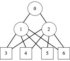
Figure 2: The physical topology of the network and the set of available network links that can be used by the optimization framework.

Figure 2 illustrates the physical layer of the network. The following conventions are used: circle are switches, square are hosts, and black lines are physical connections. It features 3 SDN appliances, nodes $0$, $1$ and $2$ that route traffic as well as block it (act as firewalls). The toy network features 4 hosts, $3$ through $6$.

src $\rightarrow$ dst	type	value
0 $\rightarrow$ 3	A	$$$
3 $\rightarrow$ 4	A	$
3 $\rightarrow$ 4	B	$
3 $\rightarrow$ 5	A	$$
3 $\rightarrow$ 5	B	$
5 $\rightarrow$ 6	A	$$

Preconditions	post
($3$,$A$)	($3$,$\mathtt{Code}$)
($5$,$A$)	($5$,$\mathtt{Code}$)
($6$,$A$), ($5$,$\mathtt{Code}$)	($6$,$\mathtt{Code}$)
($4$,$B$), ($3$,$\mathtt{Code}$)	($4$,$\mathtt{Code}$)

Table 1: Flows (left) and exploits (right) in the network in Figure 2.

Table 1 shows the required flows and security vulnerabilities in the network. This physical network must be configured to serve traffic demands. Table 1 shows a collection of data flows in the form $s\rightarrow t$ which a flow from node $s$ to node $t$. Each data flow has a type (here $A$ or $B$). Each data flow carries an economic value shown by the number of $\$$ signs.

Table 1 also shows exploits. A pair $(h,p)$ indicates the adversary has privilege $p$ on host $h$ where privileges are in $\{A,B,\mathtt{Code}\}$. The attacker can have three types of privileges, the ability to: 1) send traffic of type $A$, 2) send traffic of type $B$ or 3) execute code, denoted as $\mathtt{Code}$. Exploits have one or more pre-conditions that must be met to achieve the new privilege. Privilege level $\mathtt{Code}$ indicates the ability to execute code on that host. For the toy example, we assume all exploits have probability $1$ of being achieved if preconditions are met.

Figure 3 conveys the attack graph for this network which is built by combining the flows and exploits in Table 1. Figure 3 shows how an attacker can gain privileges using either flows that exist in the network or exploits. Figure 3 uses the following conventions: 1) circle nodes are (host,privilege) states, 2) green square NET nodes represent network reachability, 3) diamond nodes are exploits, 4) black arcs correspond to network connection, 5) incoming red links are precondition states of exploits, and 6) outgoing red links are postcondition states of exploits.

To illustrate, there is a required flow between host $0$ and host $3$ of type $A$. So precondition $(0,A)$ yields postcondition $(3,A)$. This is shown as a NET connection. A vulnerability on host $3$ transforms the $(3,A)$ precondition into the $(3,\mathtt{Code})$ postcondition. This is shown in the exploit 0 diamond in Figure 3. Note that exploits $2$ and $3$ require the attacker to have two preconditions to gain the new postcondition.

Figure 3: Attack graph for network in Figure 2.

The goal of Fashion is to configure SDN rules to minimize the impact of known attacks without unnecessarily sacrificing functionality. Specifically, each output of Fashion is a set of routing tables for each SDN appliance (including explicit firewalls). Here we focus on Fashion’s decision of which flows to serve, this corresponds to deciding which if any edges of the attack graph to cut.

We now discuss how Fashion would operate in the setting that functionality or security was considered followed by a joint setting where both were considered.

• Functionality Only All flows would be routed in the network and the attacker would be able to gain $\mathtt{Code}$ privilege on nodes $3$ through $6$.

• Security Only The most effective way to prevent the attacker from gaining $\mathtt{Code}$ privilege is to have node $0$ add a firewall rule blocking all traffic destined for node $3$ of type $A$. This corresponds to cutting edge $a$ in Figure 3. In this configuration, the internal traffic proceeds unabated. However, the high value of flow $(0,A)\rightarrow(3,A)$ was not respected doing great damage to the value of the network service.

• Balanced Configuration A balanced configuration continues to serve flow $(0,A)\rightarrow(3,A)$ because of its economic value. However, one can prevent the adversary from achieving $\mathtt{Code}$ on machines $4,5$ and $6$ by sacrificing two of the flows in Table 1. Specifically, the SDN devices add block rules to prevent routing the flows $(3,A)\rightarrow(4,B)$ and $(3,A)\rightarrow(5,A)$. This corresponds to cutting edges $b$ and $c$ in the attack graph. These two flows are chosen because of their low value in comparison to the amount of $\mathtt{Code}$ privileges they prevent the attacker from achieving.

In the above, we treat Fashion as just deciding which flows to serve, the actual framework also creates and places SDN rules on all SDN devices. That is, 1) for every required flow in the network Fashion creates routes through the topology in Figure 2 and 2) for blocked flows, Fashion ensures that traffic is routed to a firewall that drops the traffic.

Organization

The organization of this work proceeds as follows. Section 2 describes related work on the major system components. Section 3 introduces background on attack graphs and on the measures we will optimize over, Section 4 documents the optimization model, Section 5 evaluates Fashion, and Section 6 concludes.

2 Related work

Attack graphs are not a panacea, they require effort to find the necessary inputs (e.g. using a vulnerability scanner) [20, 21] and it is unclear how to implement the resulting recommendations [22] which usually correspond to some arc to cut [23]. However, cutting an arc without major damage is hard for a human analyst. Fashion is designed to address this problem. SDN provides the perfect opportunity for integration with attack graphs. SDN offers a centralized control and holistic view of the network no longer requiring external scanning tools to discover reachability data [24].

Attack graphs grow much faster than the underlying network (see Table 2), which affects analysis time. As we discuss in Section 3, we use an attack graph representation that is amenable to larger networks. Assessment of risk in an attack graph is a complex task.

Researchers have proposed high-level SDN programming languages in order to efficiently express packet-forwarding policies and ensure correctness when dealing with overlapping rules [15, 25]. These languages focus on parallel and sequential composition of policies to ensure modularity while providing correctness guarantees. When Fashion proposes a set of new rules for the controller it is important to change routing while minimizing loss [26].

To aid in network configuration, research tools assess network reachability [27], network security risk [28, 29], and link contention [30, 31]. These tools assess the quality of a configuration with respect to a single property and do not provide recommendations.

Recent tools generate network configurations from a set of functional and security requirements [32, 33, 34, 35, 36]. Captured security requirements include IPSec tunneling, allowing only negotiated packet flows, and ensuring identical rule sets on all firewalls.

Our work can be seen as unifying three recent works, one by Curry et al. [37], one by Frigault et al. [38, 18] and another by Khouzani et al. [7]. Curry et al. proposed an optimization framework for deciding on a network configuration based on the given desired network functionality of data flows and the underlying physical network. Curry et al. produce network configurations that meet all demands while blocking adversarial traffic. Each network node has an input risk and nodes assume a fraction of the risk of any node with which they share a path. Their risk measure does not consider adversaries that pivot in the network. To address this shortcoming we consider two risk measures in prior work, an declarative measure of Frigault et al. and an optimization based measure of Khouzani et al.

Frigault et al. [38, 18] present a risk assessment metric that assumes independence of compromise events. Specifically, if an adversary has two possible ways to reach some node, their total probability of reaching that node is the sum of the probability of the two paths minus the product of the two probabilities. If the adversary must obtain two capabilities to capture a node, the probability is the product of the two probabilities. This calculation is precise if compromise probabilities are independent. Frigault et al. present no timing information on their algorithm only scaling to six node attack graphs. Looking forward, we use this algorithm as a baseline for assessing the risk in our candidate configurations. Even with the assumption of independence, Frigault et al.’s metric can take minutes to compute on networks with 200 devices (see Section 6), this timing is based on an our implementation of this algorithm which has been open-sourced with the rest of Fashion.

Khouzani et al. [7] created an optimization engine designed to minimize security risk as represented by an attack graph. They show how to formulate the most effective path of an attack graph using a linear program. Their functionality view is limited to imparting an explicit numeric functional cost to each remedial action. It is unclear how to create these costs. Additionally, the size of Khouzani et al.’s optimization model grows exponentially in the size of the network, making it intractable for all put the smallest networks.

The primary technical gap in integrating these three works is creating an optimization model that effectively assesses risk in an attack graph representation that scales to moderate size networks.

Chia’s [39] subsequent model and evaluation are nearly identical to ours, so we do not compare with their results.

3 Attack Graphs

Fashion’s goal is to balance the functionality and security needs of the network. Functionality needs are relatively straightforward to state: a set of desired network flows that should be carried in the network while respecting link constraints such as bandwidth.

For security needs, we use the abstraction of attack graphs. Attack graphs model paths that an attacker could use to penetrate a network [28, 40, 41, 42]. Paths combine network capabilities such as routing and exploitation of a software/hardware vulnerabilities. An attack graph assumes an attacker starts at some entry point such as a publicly facing Web page and through a series of privilege escalations and network device accesses pivots to eventually reach his or her desired destination. (The technology supports an arbitrary starting point if one wishes to consider insider attacks.)

Two common graph representations are an attack dependency graph and an attack state graph. In the dependency view each node represents an exploit or a capability in the network and a Boolean formula over prerequisites determines whether an attacker may achieve a capability (see Fig 3). The main drawback of this representation is that the analysis of overall risk is difficult. In the state graph view, each node represents an attacker’s current capabilities. This representation eliminates cycles which simplifies analysis.

However, the representation is exponentially larger than the corresponding dependency graph. Consider a system in which $k$ abstract capabilities must be encoded. In a dependency graph, one needs $k$ nodes, one per capability. In a state graph, one needs $2^{k}$ nodes. Each node denotes the set of capabilities secured by the attacker and an arc between two states encodes the acquisition of a capability (one never “loses” a capability). This exponential blowup is prohibitive even for moderate size networks [43]. Khouzani [7] requires the state representation to model and minimize risk. The sheer size of attack state graphs prompts us to adopt the attack dependency graphs representation.

In the dependency view, each node captures an exploit or capability in the network. It may be possible to reach a capability using many different paths. Furthermore, multiple conditions may be necessary to achieve this capability, for example, network reachability of a database machine and a SQL injection attack. This is the view presented in Figure 3.

Each exploit has an associated Boolean structure (indicating when the exploit can be obtained) and a probability (indicating attacker success rate in carrying out the exploit). Capability nodes are annotated with an impact value that signifies the cost of an adversary achieving that capability (following the NIST cybersecurity framework guidance [44]). In this work, we focus on exploits that are AND and OR prerequisites (and not arbitrary Boolean formulae). Intuitively, an AND node means the attacker must have all prerequisites to achieve the new capability. An OR node means the attacker must have a single prerequisite to achieve the new capability.

While a dependency representation is compact, risk analysis is delicate. Even if one assumes that probability associated with each arc is independent, calculating the overall probability requires considering all paths, a tall order in the presence of cycles. We return to this problem after introducing prior work on quickly evaluating attack graphs and formalizing the state graph representation.

Prior work on evaluating related attack graphs

The ability to perform this analysis quickly is critical to utilize attack graphs in our optimization framework. The ability to regenerate the attack graph multiple times at decreased cost has been addressed recently in related contexts.

Almohri et al. [45] considered an attack graph setting where the defender has incomplete knowledge of the network. An example source of stochasticity is mobile device movement. Their attack graph model can capture risk subject to such stochasticity sources. This is an orthogonal consideration to our work that could be folded into Fashion’s framework as part of future work.

Frigault et al. [38, 18] and Poolsappasit et al. [3] argue that it is inaccurate to measure probabilities with a fixed probability of exploit. They argue that factors such as patch availability will decrease the threat while widespread distribution of vulnerability details may increase the threat. As such, they conduct attack graph analysis where the graph is static but probabilities can change over time. If one is willing to consider a complete attack graph then all changes in the graph can be represented with a change in probability. However, this also introduces an exponential blowup as one needs to consider an arc between each subset of nodes.

Khouzani et al. [7] is the only work that considers defensive actions that can drastically change the attack graph and a formulation of the risk calculation graph that is amenable to optimization. However, their model is inherently tied to the state graph representation.

3.1 Formalizing the problem

Building an attack graph requires network reachability information, device software configurations and known exploit information [5, 46, 47, 48] to generate the graph. Attack graphs are effective in measuring how an attacker would traverse using known vulnerabilities and system state. One can also consider the implications of a new vulnerability [9].

This section defines the risk measure used as ground truth when evaluating Fashion solutions. The metric is drawn from Frigault et al. [18] augmented with impact for each node. Frigault et al.’s metric assumes an attack graph where the probability of achieving each exploit is independent. Since paths in an attack graph often overlap, the probability of achieving prerequisites of an exploit may not be independent. This simplifying assumption is often used since considering correlated probabilities makes the problem significantly harder [49].

In isolation a misconfigured device which allows unauthorized access may be benign but when coupled with network access to ex-filtrate data or pivot to additional targets the results can be devastating. The goal of constructing and analyzing an attack graph is to understand the security posture in total. An attack graph should allow one to understand defensive weaknesses and critical vulnerabilities in the network. Since all enterprises have limited budgets, the goal of this analysis is usually to prioritize changes that have the largest impact.

An attack graph $G(N,E)$ is a directed graph. Let $\mathsf{EX}=\mathsf{EX_{n}}\cup\mathsf{EX_{v}}$ be the set of all exploits where $\mathsf{EX_{n}}$ represents the network reachability exploits (changes that can be made by the SDN controller) and $\mathsf{EX_{v}}$ represents the set of vulnerabilities. We rely on the following assumptions:

• That $\mathsf{EX}=\mathsf{EX_{AND}}\cup\mathsf{EX_{OR}}$, i.e., the set of exploits can be partitioned into conjunctive or disjunctive nodes.

• That $\mathsf{EX_{n}}\subseteq\mathsf{EX_{OR}}$, i.e., reachability is treated as OR between multiple traffic types among hosts.

• Exploits $\mathsf{ex}\in\mathsf{EX}$ are labelled with a probability $p(\mathsf{ex})$ of exploitability given that all prerequisites have been satisfied. It can be estimated using vulnerability databases [5, 46, 47]. Note that $p(\mathsf{ex})$ is a component metric, we seek to capture the cumulative risk in the network (see discussion in [18, 50]).

Let $\mathsf{C}$ be the set of all capabilities in the network. A capability $\mathsf{C}$ carries an impact, denoted as $\mathsf{Impact}(\mathsf{C})$ which is nonnegative. Let $N=\mathsf{EX}\cup\mathsf{C}$ denote the node set. Let $E=R_{r}\cup R_{i}$ denote the arc set with

• $R_{r}\subseteq\mathsf{C}\times\mathsf{EX}$ : the exploit’s prerequisites.

• $R_{i}\subseteq\mathsf{EX}\times\mathsf{C}$ : capabilities gained from an exploit.

There are no arcs in $\mathsf{C}\times\mathsf{C}$ or $\mathsf{EX}\times\mathsf{EX}$. Let $\mathsf{Start}\subseteq\mathsf{C}$ denote a set of capabilities that the adversary is believed to have. For any node $n$, $\mathsf{Pred}(n)=\{v|(v,n)\in E\}$ denotes all its predecessors in $G$, while $\mathsf{Succ}(n)=\{v|(n,v)\in E\}$ denotes all of its successors.

Risk without Cycles

First, consider how to compute risk in the absence of cycles, we follow Frigault et al..’s [18] methodology which is centered on Bayesian inference, augmented with an impact for each capability node.

The primary goal is to compute cumulative scores $P(\mathsf{ex})$ and $P(c)$ for each node in $G$. The cumulative scores $P$ are computed using the attack graph and the component score of each exploit, denoted as $p(\mathsf{ex})$.These represent the likelihood that an attacker reaches the specified node in the graph. From these scores one may consider the overall risk:

$$\mathsf{Risk}(G)=\sum_{c\in C}P(c)*\mathsf{Impact}(c)$$ (1)

$P(\cdot)$ is computed as follows in the acyclic case:

AND nodes

For AND nodes, the cumulative score is the product of $P(c)$ for all predecessors and $p(\mathsf{ex})$. The intuition is that each prerequisite must be achieved and the probabilities are assumed to be independent.

OR nodes

For OR nodes, the cumulative score is the sum of all predecessors component score minus the product of each pair of probability scores (using Bayesian reasoning). All capability nodes are treated as OR nodes. For a set $X$, we define the operator $\mathsf{Bayes}:X\rightarrow[0,1]$ as:

$$\mathsf{Bayes}(X)=\begin{cases}\sum_{X^{\prime}\subseteq X}\left(-1\right)^{|X^{\prime}|+1}\prod_{x\in X^{\prime}}p(x)&X\neq\emptyset\\ 0&X=\emptyset\end{cases}.$$

$\mathsf{Bayes}(X)$ measures the probability that at least one event in $X$ occurs (events in $X$ is assumed to be independent).

Definition 1 (Network Risk).

[18, Definition 2] Given an acyclic attack graph $G$ and any component score assignment function $p:\mathsf{EX}\longrightarrow\left[0,1\right],$ the cumulative score function $P:\mathsf{EX}\cup\mathsf{C}\longrightarrow\left[0,1\right]$ is defined as

$$P(\mathsf{ex}) =\begin{cases}p(\mathsf{ex})\cdot\prod_{c\in\mathsf{Pred}(\mathsf{ex})}P(c)&\mathsf{ex}\in\mathsf{EX_{AND}}\\ p(\mathsf{ex})\cdot\mathsf{Bayes}(\mathsf{Pred}(\mathsf{ex}))&\mathsf{ex}\in\mathsf{EX_{OR}}\end{cases}$$

$$P(c) =\begin{cases}1&c\in\mathsf{Start}\\ \mathsf{Bayes}(\mathsf{Pred}(c))&\text{otherwise}.\end{cases}$$

$P(n)$ can be computed for all $n\in N$ as long as $G$ is acyclic. This is because $P(n)$ can be computed once $P(e)$ is known for all $e\in\mathsf{Pred}(n)$. For all acyclic $G$ there is a topological ordering that allows this computation (and all topological orderings result in the same computation).

Frigault et al. [18] present a complex algorithm to handles cycles; it involves repeated, recursive evaluation of network risk on the graph with arcs removed to break cycles. Frigault et al. [18] observed that:

1. We only need to measure the probability for the first visit of a node. Consider a cycle with only one incoming arc. The arc closing the cycle can be ignored.

2. Cycles with multiple entry points are more delicate to handle and require the removal of an arc from the graph. The key insight is no path that an attacker traverses will actually follow the cycle. Different paths will include subsets of arcs from the cycle.

Frigault et al. [18] propose the following methodology for handling cycles with multiple entry points. Assume that all nodes that can be topologically sorted have been and their cumulative probabilities are assigned. Let $X$ be a cycle with at least two entry points. For each entry point $x\in X$ one can compute $P(x)$ without considering $\mathsf{Succ}(x)$. While $x$’s successors are important in calculating the overall risk they do not impact $P(x)$. Compute a new attack graph $G^{\prime}$ which has all $\mathsf{Succ}(x)$ removed and use it to calculate $P(x)$. Importantly, the graph $G^{\prime}$ may still have cycles which inhibit computation of $P(x)$ requiring this process to be repeated for all entry points in the cycle. Once all entry points have their likelihood, the rest of the cycle can be safely evaluated.

When we use the term $\mathsf{Risk}(G)$ it refers to this full computation. $\mathsf{Risk}$ is too slow to directly use for the security layer (see Section 5). A Python implementation of Frigault et al.’s algorithm [18] has been open-sourced along with the rest of Fashion [14].

3.2 Approximating Risk

To incorporate cumulative risk into an optimization framework, we turn to approximations of risk that can be linearized. The risk calculation presented in Definition 1 and its augmentation for handling cycles is non-linear and has no closed form. We consider two approximations to serve as proxies called Reachability and Max attack. We defer the evaluation of the quality of our measures to Section 5.

3.2.1 Reachability

We binarize probability of exploitation resulting in a metric called $\mathsf{Reach}$.

$$P^{*}(n)=\begin{cases}1&P(n)>\theta\\ 0&P(n)\leq\theta\end{cases}$$

The value $\theta$ is a threshold used to determine whether a capability should either be ignored or considered attained. We consider $\theta=0$. Since $p(n)\in\{0,1\}$, we can apply standard Boolean linearization techniques to get a tractable representation of dynamic risk.

$$\mathsf{Reach}(G^{*})\overset{def}{=}\sum_{c\in C}P^{*}(c)*\mathsf{Impact}(c)$$ (2)

Utilizing the binary representation of exploits in Equation 2 is an approximation, measuring how an attacker can impact a target network. Since we consider $\theta=0$ this measures the total impact of nodes reachable by the adversary. This is equivalent to calculating the weighted size of the connected components in $G$ that contains the attacker’s starting posture. The first generation of attack graphs measured this quantity [40, 51]. This models the worst case approach when calculating attacker compromise of network capabilities. Note that one can set some threshold for mapping a probability to $1$ rather than all nonzero probabilities.

This approach does have a weakness when the goal is to jointly optimize functionality and security. Consider two nodes $a$ and $b$ where $\mathsf{Impact}(a)=2*\mathsf{Impact}(b)$. Further suppose, at least $a$ or $b$ must remain in the connected component to satisfy functionality demands. The reachability metric will prioritize disconnecting $b$. However, it may be that the attacker is less likely to reach $b$. This may be the case even if $p(b)\geq p(a)$ (it is possible that $P(a)>P(b)$ due to the likelihood of reaching their predecessors).

3.2.2 Most Likely Path

The second risk measurement we introduce is the attacker’s most likely course of action, called $\mathsf{Path}$. This measure is based on Khouzani et al.’s most effective attack measure [7].

Let $\sigma$ be the attacker’s starting point in the attack graph. We define $\omega_{\sigma\rightarrow c}$ to be the set of all paths, where a path is sequence of arcs $(e_{1},\dots,e_{k})$ such that $e_{i}\in E$, from $\sigma$ to $c$ in the attack graph. Let $\Lambda_{c}\in[0,1]$ be the normalized impact of an attacker obtaining capability $c$. Then the most effective attack path is defined as follows.

$$\mathsf{Path}(G)=\max\limits_{c\in\mathsf{C}}\Lambda_{c}\max\limits_{\omega_{\sigma\rightarrow c}}\prod_{e\in\omega_{\sigma\rightarrow c}}p(\mathsf{Pred}(e))$$ (3)

Instead of having multiple targets, an auxiliary target $\mu$ is considered, that will be the sole target capability of the attacker. To do this, arcs from each $c\in\mathsf{C}$ to an auxiliary exploit $\mathsf{ex}_{c}$ are introduced, such that $p(\mathsf{ex}_{c})=\Lambda_{c}$. Then we introduce an arc from each $\mathsf{ex}_{c}$ to $\mu$. Doing this, we can reformulate equation 3 as:

$$\mathsf{Path}(G)=\max\limits_{\omega_{\sigma\rightarrow\mu}}\prod_{e\in\omega_{\sigma\rightarrow\mu}}p(\mathsf{Pred}(e))$$ (4)

However network defenses can be deployed in order to reduce the probabilities of these exploits. Let $x_{d}\in\{0,1\}$ be a binary decision variable denoting whether a network defense $d$ has been deployed. Let $p_{d}(\mathsf{ex})$ be the reduced probability of exploit $\mathsf{ex}$ due to network defense $d$. With this, the probability of exploit $\mathsf{ex}$ with respect to network defense decision $x_{d}$ is given by

$$p_{x_{d}}(\mathsf{ex})=p(\mathsf{ex})(1-x_{d})+p_{d}(\mathsf{ex})x_{d}.$$ (5)

We will minimize the risk due to the most effective path risk over all the possible configurations of network defenses available. This approach identifies appropriate locations to deploy network defenses to protect both high value capabilities with low exploitability as well as lower value, more exploitable assets. We will incorporate these defense decisions when defining our optimization model in Section 4.

$\mathsf{Path}$ does not distinguish between a graph with $2$ paths with the same underlying probability and a single path with that probability. In addition to this inaccuracy (that was present in Khouzani et al’s work) working on the attack dependency graph introduces two sources of error:

1. $\mathsf{Path}$ only counts the impact from the last node on the path. This is because it is only measuring the probability of a path and the impact is added as a “last layer” in the graph. So it does not distinguish between two paths (of equal probability) where one path has intermediate nodes with meaningful impact. In the attack state representation each node has the current capabilities of the attack and thus impact of this node set can be added as a last layer.

2. The path used to determine $\mathsf{Path}$ may not be exploitable by an adversary due to exploit nodes with multiple prerequisites. That is, the path may include a node with multiple prerequisites and the measure only computes the probability of exploiting a single prerequisite. In the attack state representation there are no nodes with multiple prerequisites so this problem does not arise.

3.2.3 Averaging $\mathsf{Reach}$ and $\mathsf{Path}$

As described above both $\mathsf{Reach}$ and $\mathsf{Path}$ have weaknesses. We demonstrate in Section 5 that Fashion outputs better solutions when considering both metrics. We call the weighted sum of these two functions $\mathsf{Hybrid}$.

$\mathsf{Reach}$ isolates nodes that do not need to communicate. When deciding which of two flows to route, $\mathsf{Reach}$ may not make the right decision as it cannot quantitatively distinguish between the risk of these flows. However, in this case $\mathsf{Path}$’s measure can break ties as it includes probability of exploitation while $\mathsf{Reach}$ does not.

$\mathsf{Path}$ is effective at isolating nodes that have a high probability path to them. Yet, this measure does not account for the other nodes compromised “on the way” to the target node. By minimizing the total weighted reachable set using $\mathsf{Reach}$ this weakness is partially mitigated. Similarly, if two paths have similar probability but one contains multiple AND prerequisites, it may have a larger reachable component, enabling $\mathsf{Reach}$ to again break ties.

4 Optimization Model

This section highlights the content and structure of the optimization model used to obtain network configurations that uphold a balance between functionality and security. The optimization model is a binary integer programming (BIP) model as all decision variables are binary. The model contains two components dedicated, respectively, to the modeling of the data network and its job as a carrier for data flows and to the representation of the attack graph and the modeling of induced risk measures $\mathsf{Reach}$ and $\mathsf{Path}$. The core decision variables fall in two categories.

First, Boolean variables model the routing decisions of the data flows in the network. Such a variable is associated to each network link and subjected to flow balance equations as well as link capacity constraints. They also contribute to the functional rewards (in the objective) associated to the deliveries of the flow values.

Second, Boolean variables are associated to the deployment of counter-measures in the network. In this work, counter-measures are routing a flow to a firewall (rather than its destination). Auxiliary Boolean variables facilitate the expression of the model and setup channeling constraints that tie the attack graph model to the network routing model so that routing as well as blocking decisions are conveyed to the attack graph part of the model and result in severing arcs that express pre-conditions of exploits.

While the constraints devoted to capturing reachability, i.e., $\mathsf{Reach}$, are relatively straightforward, the modeling of the most effective path, i.e., $\mathsf{Path}$ is more delicate for two reasons. First, it requires the use of products of probabilities held in variables yielding a non-linear formulation. Thankfully, that challenge can be side-stepped by converting those products into sums with a logarithmic transform. Second, it delivers a $\min-\max$ problem that needs to be dualized to recover a conventional minimization.

4.1 Full Model

In binary integer programming, the four primary components are Inputs, Variables, Constraints, and an Objective function. These are listed below.

4.1.1 Inputs

$\mathcal{R}$ – the set of SDN devices (routers/firewall).
$\mathcal{H}$ – the set of hosts (machines) on the network.
$\mathcal{G}\subset\mathcal{R}$ – the set of external gateway devices in the network.
$\mathcal{D}=\mathcal{R}\cup\mathcal{H}$ – the set of all network devices.
$\mathcal{L}\subset D\times D$ – the set of all network links.
$\mathcal{T}$ – the set of traffic types.
$\mathcal{F}$ – the set of tuples $(h,k,t)\in\mathcal{D}\times\mathcal{D}\times\mathcal{T}$ defining desired traffic flows of type $t$ from source device $h$ to sink device $k$.
$s^{*}$ – an artificial node in the network used as the global source of all flows.
$t^{*}$ – an artificial node in the network used as the global destination of all flows.
$\sigma$ – an artificial node in the attack graph used as the global starting point of the attacker.
$\mathsf{C}$ – the set of capabilities an attacker could gain on devices in $\mathcal{D}$.
$\mathsf{Start}$ – the set of starting capabilities for an attacker.
$\mathsf{EX_{n}}$ – the set of exploits based on network connections.
$\mathsf{EX_{v}}$ – the set of exploits based on network vulnerabilities.
$\mathsf{EX_{AND}}$ – the set of AND exploits.
$\mathsf{EX_{OR}}$ – the set of OR exploits.
$\mathsf{EX}=\mathsf{EX_{n}}\cup\mathsf{EX_{v}}=\mathsf{EX_{AND}}\cup\mathsf{EX_{OR}}$ – the set of all exploits.
$Q(l):\mathcal{L}\rightarrow\mathbb{R}$ – the capacity of link $l$.
$K(i):\mathcal{R}\rightarrow\mathbb{R}$ – the capacity of network device $i$.
$\tau(f):\mathcal{F}\rightarrow\mathcal{T}$ – yields the traffic type of flow $f$.
$\tau(\mathsf{ex}):\mathsf{EX_{n}}\rightarrow\mathcal{T}$ – yields the traffic type of network exploit $\mathsf{ex}$.
$p(\mathsf{ex}):\mathsf{EX}\rightarrow[0,1]$ – the probability of success for a given exploit.
$\delta^{-}(i):\mathcal{D}\rightarrow 2^{\mathcal{D}}$ – the set of vertices with outbound arcs leading to vertex $i$.
$\delta^{+}(i):\mathcal{D}\rightarrow 2^{\mathcal{D}}$ – the set of vertices with inbound arcs originating at vertex $i$.
$\mathsf{Pred}(n):N\rightarrow 2^{N}$ – set of the predecessors of $n$ in the attack graph.
$\mathsf{Succ}(n):N\rightarrow 2^{N}$ – set of the successors of $n$ in the attack graph.
$\textsf{src}(f)\in\mathcal{D}$ – the network device source of flow $f$.
$\textsf{dst}(f)\in\mathcal{D}$ – the network device destination of flow $f$.
$\textsf{q}(f):\mathcal{F}\rightarrow\mathbb{R}$ – the quantity of data attributed to flow $f$.
$\textsf{val}(f):\mathcal{F}\rightarrow\mathbb{R}$ – the value of flow $f$.
$\textsf{dev}(c):\mathsf{C}\rightarrow\mathcal{D}$ – yields the device in a capability node.
$\textsf{dev}(\mathsf{ex}):\mathsf{EX_{n}}\rightarrow\mathcal{D}$ – yields the destination device of a network-connection-based exploit.
$\textsf{cost}(l):\mathcal{L}\rightarrow\mathbb{R}$ – the cost of an arc in the network.
$\mathsf{Impact}(c):\mathsf{C}\rightarrow\mathbb{R}$ – the impact of attack gaining capability $c$.

4.1.2 Variables

$\rho_{i,j}^{f}\in\{0,1\}$ – for every $f\in\mathcal{F}$ and every $(i,j)\in\mathcal{L}$, indicates whether link $(i,j)$ carries flow $f$.
$b_{i}^{f}\in\{0,1\}$ – for every $f\in\mathcal{F}$ and every $i\in\mathcal{R}$, indicates whether flow $f$ is blocked by a firewall at network device $i$.
$w_{i}^{f}\in\{0,1\}$ – for every $f\in\mathcal{F}$ and every $i\in\mathcal{R}$, indicates whether there is a firewall filtering flow $f$ at network device $i$.
$v_{i}^{t}\in\{0,1\}$ – for every $t\in\mathcal{T}$ and every $i\in\mathcal{R}$, indicates whether there is a firewall blocking traffic type $t$ at network device $i$.
$W_{i}\in\{0,1\}$ – for every $i\in\mathcal{D}$, indicates whether there is any kind of firewall present at network device $i$.
$N_{k,h}^{t}\in\{0,1\}$ – for every $(k,h)\in(\mathcal{H}\cup\mathcal{G})\times\mathcal{H}$ and every $t\in\mathcal{T}$, indicates whether there is an active network connection between devices $h$ and $k$.
$\beta_{i}^{f}\in\{0,1\}$ – for every $i\in\mathcal{R}$ and every $f\in\mathcal{F}$, indicates whether network device $i$ blocks flow $f$ using a firewall specific to traffic type.
$\theta_{i}^{f}\in\{0,1\}$ – for every $i\in\mathcal{R}$ and every $f\in\mathcal{F}$, indicates whether network device $i$ receives flow $f$.
$r_{n}\in\{0,1\}$ – for every $n\in\mathsf{C}\cup\mathsf{EX}$, indicates whether node $c$ is reachable from the root of the attack graph.
$a_{i,j}\in\{0,1\}$ – for every $(i,j)\in E$, indicates whether arc $(i,j)$ is present (i.e., not cut) in the attack graph.
$x_{i,j}\in\{0,1\}$ – for every $(i,j)\in E$, indicates whether an attacker would be able to traverse arc $(i,j)$, i.e., $r_{i}\land a_{i,j}$.

4.1.3 Functionality Constraints

The first part of the model captures the networking side of the model, including how to route flows, respect capacities of devices and how to block specific flows.

$$\rho^{f}_{s^{*},src(f)}=1,\>\>\forall f\in\mathcal{F}$$ (6)

Equation 6 forcibly spawns each flow in the network at its network machine source.

$$\beta_{i}^{f}=\theta_{i}^{f}\land v_{i}^{\tau(f)},\>\>\forall f\in\mathcal{F},\forall i\in\mathcal{R}$$ (7)

$$b_{i}^{f}=w_{i}^{f}\lor\beta_{i}^{f},\>\>\forall f\in\mathcal{F},\forall i\in\mathcal{R}$$ (8)

Equation 7 models that a flow $f$ is blocked at device $i$ if it reached device $i$ and a firewall rule blocked traffic of the type carried by $f$. Equation 8 is similar, but states that a flow $f$ is blocked if there is a firewall rule specifically designed to drop flow $f$ or if it was blocked by a generic firewall type rule.

$$\theta_{i}^{f}=\bigvee\limits_{j\in\delta^{-}(i)}\rho_{j,i}^{f},\>\>\forall f\in\mathcal{F},\forall i\in\mathcal{R}$$ (9)

Lastly, equation 9 states that a flow $f$ arrives at device $i$ if one of the inbound arcs into $i$ carries flow $f$.

$$\sum\limits_{j\in\delta^{-}(i)}\rho_{j,i}^{f}=\sum\limits_{k\in\delta^{+}(i)}(\rho_{i,k}^{f}+\beta_{i}^{f}),\>\>\forall f\in\mathcal{F},\forall i\in\mathcal{R}$$ (10)

$$\sum\limits_{j\in\delta^{-}(i)}\rho_{j,i}^{f}=\sum\limits_{k\in\delta^{+}(i)}\rho_{i,k}^{f},\>\>\forall f\in\mathcal{F},\forall i\in\mathcal{H}$$ (11)

Equations 10 and 11 are the flow balance equations that dictate that every inbound flow must also be outbound, unless it was blocked. The equations are slightly different for internal SDN devices (equation 10) and hosts that are not permitted to route traffic (equation 11).

$$\rho_{i,j}^{f}=0,\>\>\forall f\in\mathcal{F},\forall i\in\mathcal{H}\setminus\{\textsf{src}(f),\textsf{dst}(f)\},\forall j\in\delta^{+}(i)$$ (12)

$$\rho_{\textsf{dst}(f),j}^{f}=0,\>\>\forall f\in\mathcal{F},\forall j\in\delta^{+}(i)\setminus\{t^{*}\}$$ (13)

Equations 12 and 13 states that hosts can only forward traffic to the flow sink by preventing the use of any other outbound arc.

$$\sum\limits_{f\in\mathcal{F}}(\rho_{i,j}^{f}\cdot q(f))\leq Q(i,j),\>\>\forall(i,j)\in\mathcal{L}$$ (14)

$$\sum\limits_{f\in\mathcal{F}}\sum\limits_{k\in\delta^{-}(i)}(\rho_{k,i}^{f}\cdot q(f))+\sum\limits_{f\in\mathcal{F}}\sum\limits_{j\in\delta^{+}(i)}(\rho_{i,j}^{f}\cdot q(f))\leq K(i),\>\>\forall i\in\mathcal{R}$$ (15)

Equation 14 simply models the bounds on link capacities. Equation 15 plays a similar role for the device capacities.

$$W_{i}=\bigvee\limits_{f\in\mathcal{F}}w_{i}^{f}\vee\bigvee\limits_{t\in\mathcal{T}}v_{i}^{t}\>\forall i\in\mathcal{R}$$ (16)

Equation 16 models the existence of a blocking firewall of any kind at SDN device $i$.

$$N_{k,h}^{t}=\begin{cases}\rho_{h,t^{*}}^{f}&\mbox{ if }\langle k,h,t\rangle\in\mathcal{F}\\ 0&\mbox{otherwise}\end{cases},$$ (17)

$$\>\>\forall(h,k)\in(\mathcal{H}\cup\mathcal{G})\times\mathcal{H},\forall t\in\mathcal{T}$$

Equation 17 models the existence of an active network connection between devices $k$ and $h$.

Now, using the above constraints, we will derive a functionality score $\mathcal{O}_{f}$ for the network configuration. Looking ahead, this score will be used in defining the overall objective for the model.

$$\mathcal{O}_{f} =\>\>\alpha_{0}\sum\limits_{f\in\mathcal{F}}-\rho_{dst(f),\mu}\cdot\textsf{val}(f)$$

$$+\alpha_{1}\sum_{f\in\mathcal{F}}\sum_{(i,j)\in\mathcal{L}}\rho_{i,j}^{f}\cdot\textsf{cost}(i,j)$$ (18)

The first term yields a credit for routing good flows through the network from their source to their destination and is scaled by the assigned value of the flow. The second term describes the cost incurred by routing flows though the network based on the cost of the links use to carry each flow.

Lastly, we will use the functional constraints to derive a score for the cost of deploying network defenses, $\mathcal{O}_{d}$. This score will also appear in the objective function as part of the overall security cost.

$$\mathcal{O}_{d}=\alpha_{2}\sum_{i}w_{i}+\alpha_{3}\sum_{i}\sum_{t}v_{i}^{t}\>\>+\alpha_{4}\sum_{i}W_{i}$$ (19)

The first two terms describe the cost paid for deploying flow-specific and traffic-specific firewalls, respectively. The third term gives a penalty per unique network device deploying any kind of firewall and its a way to reduce network complexity by encouraging the concentration of multiple firewalls to a few devices.

4.1.4 Security Constraints

Here we will lay out the necessary constraints to calculate the $\mathsf{Reach}$ and $\mathsf{Path}$ attack graph metrics, which will be needed in the formulation of the objective function of our model.

$\mathsf{Reach}$ Measure

This part of the model is devoted to which capabilities an attacker can reach from the root of the attack graph. It creates channels between variables of the networking model and variables of the attack graph. It also models the semantics of AND and OR nodes as well reachability within the attack graph.

$$r_{c}=\bigvee\limits_{i\in\mathsf{Pred}(c)}x_{i,c},\>\>\forall c\in\mathsf{C}$$ (20)

$$r_{\mathsf{ex}}=\bigwedge\limits_{i\in\mathsf{Pred}(\mathsf{ex})}x_{i,\mathsf{ex}},\>\>\forall\mathsf{ex}\in\mathsf{EX_{AND}}$$ (21)

$$r_{\mathsf{ex}}=\bigvee\limits_{i\in\mathsf{Pred}(\mathsf{ex})}x_{i,\mathsf{ex}},\>\>\forall\mathsf{ex}\in\mathsf{EX_{OR}}$$ (22)

Equation 20 models an OR node. Namely, it states that the capability $n$ is enable if the adversary can traverse at least one inbound arc (coming from an exploit). Equation 21 models an AND node. Namely, it states that the exploit $n$ is enabled provided that all inbound arcs can be traversed by the adversary. Equation 22 models an OR node in a similar fashion.

$$x_{i,j}=r_{i}\bigwedge a_{i,j},\>\>\forall(i,j)\in E$$ (23)

Equation 23 enables an arc $(i,j)$ in the attack graph if its source is reachable and the arc was not cut by $a_{i,j}$.

$$a_{i,j}=1,\>\>\forall(i,j)\in\mathsf{EX_{v}}$$ (24)

$$r_{\sigma}=1$$ (25)

Equations 24 state that arcs that are incident on a vulnerability-based exploit $x$ are always enabled while equation 25 states that the attacker’s starting point $\sigma$, which has arcs leading to every $n\in\mathsf{Start}$, is always reachable.

$$a_{c,\mathsf{ex}}=N_{\textsf{dev}(c),\textsf{dev}(\mathsf{ex})}^{\tau(\mathsf{ex})},\>\>\forall c,\mathsf{ex}\textrm{ s.t. }(c,\mathsf{ex})\in E$$ (26)

Equation 26 is a channeling constraint connecting the presence of an network-connection-based arc in the attack graph to reachability in the network model. Using the constraints just defined, we can formalize a security cost based on attack graph reachability, $\mathcal{O}_{r}$, that will appear in the objective function.

$$\mathcal{O}_{r}=\sum_{n\in\mathsf{C}}r_{n}\cdot\mathsf{Impact}(n)$$ (27)

Here we consider which capabilities an attacker can reach and use the associated impact of them achieving that capability as a penalty.

$\mathsf{Path}$ Measure

This part of the model focuses on capturing an attacker’s most effective attack path, which is formulated in Equation 4, and embedding it within a minimization. To model this in a binary integer program, we use the strategy presented by Khouzani et al. [7]. First, we note that Equation 4 is equivalent to the following.

$$\max\limits_{\gamma}\prod\limits_{e\in E}(\gamma_{e}p(t(e))+1-\gamma_{e})\textrm{ s.t. }\gamma_{e}\in\{0,1\}\>\>\forall e\in E,$$ (28)

$$\sum\limits_{e:h(e)=i}\gamma_{e}-\sum\limits_{e:t(e)=i}\gamma_{e}=\begin{cases}1\>\>&\mbox{if }i=\mu\\ -1\>\>&\mbox{if }i=\sigma\\ 0\>\>&\forall i\in\mathsf{C}\cup\mathsf{EX}\\ \end{cases}$$ (29)

Here $\gamma_{e}$ is a binary decision variable that indicates whether an arc $e$ is on the most effective attack path. Equation 29 enforces that the arcs chosen will form a path from $\sigma$, the global attack graph starting point, to $\mu$, the global attack graph target. Here $h(e)$ and $t(e)$ denote the head $j$ and tail $i$ of an arc $(i,j)$. And since the objective function maximizes the probability of the taken path, as the product scales with an arc’s probability if the arc is taken and 1 otherwise, this formulation is equivalent to equation 4. However, as written, this formulation is not linear, as there is a product of variables in the objective function, and thus cannot be directly incorporated into a linear binary integer program. We can address this concern by composing the above objective with the monotonic function $\log(\cdot)$.

$$\log\prod\limits_{e\in E}(\gamma_{e}p(t(e))+(1-\gamma_{e}))=\sum\limits_{e\in E}\log(\gamma_{e}p(t(e))+(1-\gamma_{e}))$$

And considering that $\gamma_{e}\in\{0,1\}$, the above equation can be further simplified to $\sum\limits_{e\in E}\gamma_{e}\log(p(t(e))$. With this we now have the following optimization problem to model the most effective attack path.

$$\max\limits_{\gamma}\sum\limits_{e\in E}\gamma_{e}\log(p(t(e)))\textrm{ s.t. }\gamma_{e}\geq 0\>\>\forall e\in E$$ (30)

$$\sum\limits_{e:h(e)=i} \gamma_{e}-\sum\limits_{e:t(e)=i}\gamma_{e}=\begin{cases}1\>\>&\mbox{if }i=\mu\\ -1\>\>&\mbox{if }i=\sigma\\ 0\>\>&\forall i\in\mathsf{C}\cup\mathsf{EX}\\ \end{cases}$$

Now we have obtained a linear formulation for the most effective attack path, but there is one more issue to address. The formulation is a maximization that we will be minimizing when synthesizing network configurations. Formulating this problem as a min-max is not desirable, so instead of solving the above maximization problem to find the most effective attack path, we will instead solve its dual, which is a minimization problem with the same optimal solution. The dual model is given below.

$$\min\limits_{y}y_{\sigma}-y_{\mu}$$ (31)

s.t. $$y_{t(e)}-y_{h(e)}\geq\log(p(t(e)))\>\>\forall e\in E$$

Note that because of the ability to deploy network defenses, we can apply $\log(\cdot)$ to equation 5 to obtain:

$$\log(p(t(e)))=(1-x)\log(p(t(e)))+x\log(\epsilon).$$

Since we apply $\log$ to the probabilities, we cannot have an exploit with a probability of zero. Thus we use a very small number $\epsilon$ to model the scenario where network defenses reduce the likelihood of an exploit to zero. In particular, this is how completely severing host-to-host communications in the network can cut arcs incident to network reachability exploits in the attack graph. Now that we have formulated a minimization problem here, it can be incorporated directly into the objective function of our overall minimization problem as the security cost due the most effective attack path, $\mathcal{O}_{p}$,

$$\mathcal{O}_{p}=y_{\sigma}-y_{\mu}$$ (32)

4.1.5 Objective

The objective function in this model is comprised of two components, a functionality cost and a security cost. The overall functionality cost is given directly by $\mathcal{O}_{f}$ as seen in Equation 18. We will define the overall security cost $\mathcal{O}_{s}$ as a linear combination of the security costs laid out in Equations 19,27,32.

$$\mathcal{O}_{s}=\beta_{0}\mathcal{O}_{d}+\beta_{1}\mathcal{O}_{r}+(1-\beta_{1})\mathcal{O}_{p}.$$

The cost of deploying network defenses is application dependent so we do not vary $\beta_{0}$ in our experiments, setting it to a constant of $\beta_{0}=1$. One can vary $\beta_{1}$ to have the framework prefer one risk metric over the other. Finally, the overall objective that dictates a balance between functionality and security is a convex combination of the functionality and security costs:

$$\min\>\>\alpha\mathcal{O}_{f}+(1-\alpha)\mathcal{O}_{s}$$ (33)

Here we have the ability to vary $\alpha$ to influence the framework to produce network configurations that favor functionality over risk or vice versa. Two key parameters of the optimization model are, therefore, $\alpha$ and $\beta_{1}$ that control the functionality-risk tradeoff and the balance between $\mathsf{Path}$ and $\mathsf{Reach}$ measures.

4.2 Extending to an Online Setting

As stated, Fashion is suitable for deriving a network configuration that satisfies long-standing, or static, flow demands. However, in an online setting it is common for demands and exploits (discovery or patching) to change over time. In these cases, it is important to have an optimization framework that is robust in the wake of perturbations to input data.

When updating a current network configuration, Fashion should develop configurations that are functional, secure, and similar in routing to the current setup. This would prevent a major routing overhaul being caused by the addition of a single nascent demand. This section extends Fashion to take the current network state along with new demands/exploits as input and generate updated configurations.

4.2.1 Extension Inputs

$\textsf{sol}_{\rho}:\mathcal{F}\times\mathcal{L}\rightarrow\{0,1\}$ – the value of $\rho^{f}_{i,j}$ in the current network configuration.
$\textsf{sol}_{b}:\mathcal{F}\times\mathcal{R}\rightarrow\{0,1\}$ – the value of $b^{f}_{i}$ in the current network configuration.
$\textsf{sol}_{w}:\mathcal{F}\times\mathcal{R}\rightarrow\{0,1\}$ – the value of $w^{f}_{i}$ in the current network configuration.
$\textsf{sol}_{v}:\mathcal{T}\times\mathcal{R}\rightarrow\{0,1\}$ – the value of $v^{t}_{i}$ in the current network configuration.

4.2.2 Extension Variables

$\zeta$ – the number of variable assignment differences between the previous and current configurations.

4.2.3 Extension Constraints

The only constraint needed for the extension is one to calculate the number of variable assignment differences between the previous and current solutions. It is presented below in Equation 4.2.3.

$$\zeta=\ \ \sum\limits_{f\in\mathcal{F}}\sum\limits_{(i,j)\in\mathcal{A}}|\textsf{sol}_{\rho}(f,i,j)-\rho^{f}_{i,j}|$$

$$+\sum\limits_{f\in\mathcal{F}}\sum\limits_{i\in\mathcal{R}}|\textsf{sol}_{b}(f,i)-b^{f}_{i}|$$

$$+\sum\limits_{f\in\mathcal{F}}\sum\limits_{i\in\mathcal{R}}|\textsf{sol}_{w}(f,i)-w^{f}_{i}|$$ (34)

$$+\sum\limits_{t\in\mathcal{T}}\sum\limits_{i\in\mathcal{R}}|\textsf{sol}_{v}(t,i)-v^{t}_{i}|$$

4.2.4 Extension Objective

In order to guide the model towards configurations similar to the current one, the number of variable assignment differences is directly appended to the usual objective function. The complete objective function for the online FASHION variant is shown in Equation 35.

$$\min\>\>\alpha\mathcal{O}_{f}+(1-\alpha)\mathcal{O}_{s}+\zeta$$ (35)

5 Evaluation

In this section we show the efficacy and efficiency of Fashion. The goal is to understand (i) whether Fashion produces configurations that effectively balance functionality and security and (ii) whether Fashion produces configurations quickly, what time scale of events can Fashion respond to?

5.1 Experimental Setup

Network Topology					Network Traffic				Vulnerabilities
pod	Devices	Hosts	Switch	Links	#traffic		#flows		Exploits		AG arcs
					min	max	min	max	min	max	min	max
2	10	4	6	9	1	3	8	80	1	10	18	165
4	37	16	21	52	1	3	32	320	1	40	258	2350
6	100	54	46	171	1	3	108	1080	5	108	2928	26463
8	209	128	81	400	1	3	256	2560	12	250	16422	147627
10	376	250	126	775	1	2	500	1500	12	400	62537	250765
12	613	432	181	1332	1	3	866	866	21	105	186682	1677306

Table 2: Benchmark data, 649 instances. The number of links represents the number of bi-directional links in the network. The $\#$traffic column represents the number of distinct traffic types.

To the best of our knowledge, no standard benchmarks for attack graphs exist. For the purpose of this research, we created a benchmark suite with over 600 instances that models a data center topology and its traffic patterns and utilization rates, along with a realistic representation of dispersed network vulnerabilities. A high level breakdown of the benchmark characteristics can be found in Table 2. The evaluation is made on a Linux machine with an Intel Xeon CPU E5-2620 2.00 GHz and 64GB of RAM. The model implementation was built in Python 3.7 using the Gurobi optimization library [52].

Network Topology

The generated instances are of the popular Clos [53] style network topology Fat-tree [17] and are representative of a cloud data center. Fat-tree features an expanding pod structure of interconnected and tiered switches providing excellent path redundancy. The topology is designed to deliver high bandwidth to many end devices at moderate cost while scaling to thousands of hosts. Switch and link capacities in all benchmarks are 1GBps. The benchmarks include small to medium sized instances. The largest instance tested, includes 613 devices (hosts and SDN devices) and 1332 links between these.

Network Traffic

Network demand is modeled after the recent Global Cloud Index (GCI) report [54] which provides a global aggregated view of data centers. The benchmarks include two distinct traffic patterns: Internal at $70\%$ and External at $30\%$ (by combining GCIs Inter-data center $15\%$ and Internet $15\%$). Research shows that there exists heavy-tailed distributions for the volume and size of data flows [55]. There are generally small (1Mb-10Mb) and large (100Mb-1Gb) sized flows with 90% of the traffic volume being small and 10% large [56], all benchmarks follow this distribution.

Each flow is randomly labelled with a traffic type with number of types ranging from 1 to 3, and number of flows per host varying in $\{1,3,5,10\}$. Each flow is randomly labeled with a traffic type to account for the range of traffic such as HTTP,HTTPS,SMB [57]. For considered instances, the number of traffic type varies from 1 to 3.

One-third of the instances have 1 traffic type, one-third of the instances have 2 traffic types and the one-third of instances have three traffic types. Each flow is assigned a flow value at random from the set $\{1,2,3,5,25\}$. Network utilization is impacted by several factors such as time of day [58], or application distribution [59] The number of flows per host is varied across benchmarks with steps $\{1,3,5,10\}$ to vary network utilization [58, 59].

As an illustrative example of the benchmark generation process consider an instance with 54 hosts and 10 flows per host resulting in $540$ bidirectional flows. Each bidirectional flow is first randomly assigned as internal ($70\%$) or external ($30\%$). Next, the source and destination are randomly selected, two distinct hosts for internal or one host and the Gateway switch for external. (Note, the Gateway is the demarcation point between the network and the Internet) Each flow is then assigned a size, traffic type and value based on the distributions provided above. Finally, each flow is duplicated reversing the source and destination to represent two-way traffic, resulting in $1080$ total flows.

Vulnerabilities

Synthetic vulnerabilities are injected on hosts within the network. The generation adopts several components from the vulnerability model presented in the recent CVSS 3.1. Base metrics focusing on exploitability and impact [47]. The percentage of exploitable hosts ranges in $\{10\%,20\%,30\%,40\%,50\%\}$ and the average number of vulnerabilities per host (1-5) drives the total number of vulnerabilities injected. The number of vulnerabilities per host is representative of Zhang et al.’s findings [60] from scans of publicly available VMs after patching was performed.

Each vulnerability has one or more prerequisite conditions and a single post condition of privilege escalation (if successfully exploited). Each vulnerability is uniformly assigned a score $[0,1]$ representing the probability of exploitation. Three privilege levels $\{0,1,2\}$ are assumed where 0 denotes networking reachability.

Procedurally, the single precondition exploits are generated at random from selected exploitable hosts, each allowing the escalation of a single step in privilege level. The precondition of these single-precondition exploits have a probability of $.50$. If the required number of single precondition exploits exceeds the number of exploitable hosts then additional random hosts have vulnerabilities manually placed on them.

Multi-precondition exploits are generated by selecting one prerequisite randomly from the pool of existing (single precondition) exploits and generating a new exploit which increases the privilege of one of the input exploits, the other, secondary prerequisites are selected randomly. The preconditions of these multi-precondition exploits have a probability of $.25$ each. Importantly, the secondary prerequisite selection is restricted to currently reachable exploits to ensure the attack graph has large connected components. The primary prerequisite (the privilege that will be escalated) selection is not restricted to currently achievable nodes.

The impact of a successful exploit is reflective of the value of the threatened host. We uniformly assigned each host an integer in $[1,100]$ to represent its value to an organization. The impact of compromise of reaching a privilege level on a host is a percentage of this asset value. The quantities $[20\%,40\%,100\%]$ are used as the scaling factors for the three privilege levels $\{0,1,2\}$.

5.2 Results

We first focus on the basic model designed for an initial configuration, we then consider the online setting in Section 5.2.4.

5.2.1 Evaluating Fashion’s Initial Configurations

The discussion focuses on answering the three questions: 1) does Fashion produce good configurations? 2) does it do so in a timely manner? and 3) can Fashion work in an online manner? Answering the first question is slightly delicate because our security optimization is using $\mathsf{Reach}$ and $\mathsf{Path}$ instead of using $\mathsf{Risk}$. Throughout this section we only report on the security quality of the final configuration with respect to $\mathsf{Risk}$ (we view this as our baseline metric). This metric was introduced by Frigault et al. [18] for measuring risk in Bayesian attack graphs. The algorithm for computing $\mathsf{Risk}$ is too slow to use in the optimization model but allows an effective check on the quality of the solution a posteriori. In all results the functionality score is the normalized value of the delivered traffic: it considers the total value of traffic delivered when $\alpha~{}=~{}1$ (corresponding to the optimization considering only functionality) as a functionality score of $1$ with the other functionality scores normalized accordingly. $\mathsf{Risk}$ is normalized in a similar way and computes the $\mathsf{Risk}$ value when $\alpha~{}=~{}1$ (no protections deployed) and uses this as the denominator for other configurations. When $\alpha~{}=~{}1$ this corresponds to a baseline $\mathsf{Risk}$ for all trade-offs of the security model. This is because the security model is inactive in the optimization.

5.2.2 Does Fashion produce good configurations?

Section 3.2.3 argues that combining the two security models would produce better configurations than having $\beta_{1}~{}=~{}0$ or $\beta_{1}~{}=~{}1$. This was confirmed in our experiments. Setting $\beta_{1}=1$ produced a meaningful trade-off between functionality and security. However, when we consider $0<\beta_{1}<1$ in the $\mathsf{Hybrid}$ manner, solution quality improves. In all analyzed solutions, varying $\alpha$ with just the $\mathsf{Path}$ measure active ($\beta_{1}=0$) produced solutions that varied $\mathsf{Path}$ but not the actual $\mathsf{Risk}$ (other than blocking the gateway).

Thus, the setting of $\beta_{1}\in(0,1)$ seems crucial, but the particular value within $(0,1)$ does not seem to have a substantial effect on solution quality. This would be the case if one model is primarily being used as a tie-breaker for the other model. However, we cannot rule out that different settings of $\beta_{1}$ would be preferable on different classes of networks and attack graphs. For the remainder of the analysis, consider $\beta_{1}=.5$, i.e., $\mathsf{Path}$ and $\mathsf{Reach}$ are equally weighted.

Monotonicity

One can ask if Fashion produces solutions that trade off functionality and security. As a reminder, we use whitelist and source specific routing so setting $\alpha=1$ corresponds to the minimum risk that is achievable while routing all desirable flows (assuming routing all flows is feasible within bandwidth constraints). Any further minimization of risk necessitates decreasing functionality. Furthermore, since we consider an external attacker, blocking all flows at the entry point is always the solution chosen when functionality is not considered (optimizing only over risk). Thus, every instance has functionality and risk of $0$ when $\alpha~{}=~{}0$. We remove this point from all analysis and consider $\alpha~{}>~{}0$. Furthermore, we normalize both risk and functionality by $\alpha=1$ so we remove this point as well.

Since Fashion is approximating $\mathsf{Risk}$ it is possible for a decrease in $\alpha$ to lead to worse risk and functionality. However, in all of our experiments, risk and functionality were both monotonic for steps of $\alpha$ of size $.1$. We consider 212 benchmarks of pod size of 6, each having 54 hosts. Varying $\alpha$ for each benchmark we plot both the functionality scores against $\alpha$ and also the risk scores against $\alpha$. The functionality and risk scores are normalized as previously stated. Figure 4 demonstrates the probability mass functions over every instance solution varying $\alpha=.1$ to $\alpha=.9$ in steps of $.1$.

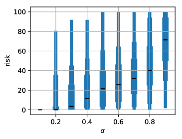
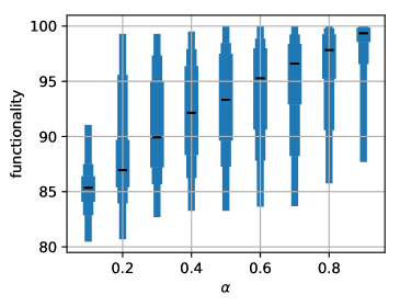
Figure 4: Probability mass function of instances for normalized risk (left) and normalized functionality (right). Start of bar represents min, widening at 10% and 25% with a line at 50%, reducing width at 75% and 90%, stopping at the max for each $\alpha$. In all cases, risk is $0$ when $\alpha=.1$. Both scores are normalized by the setting when $\alpha=1$. This corresponds to the security layer being inactive. Functionality is measured directly using Fashion’s functionality objective, $\mathcal{O}_{f}$. Because our security layer approximates risk in an attack graph, here we directly report on Frigault et al.’s [18] metric. Our security measure $\mathcal{O}_{s}$ behaved monotonically as well.

Functionality scores across all benchmarks are relatively stable for $\alpha\geq.1$ while the risk scores vary more. (The two graphs have different $y$-axes.)

Importantly, at every point on this curve Fashion is computing and outputting a corresponding network configuration. Note that in addition to considering what flows to include, the solution also describes how to route flows in a way that respects switch and link capacity. Based on visual inspection we classified our instances into three types of attack graphs.

Instances where exploitable hosts are critical In such instances nodes with exploits serve as destinations in many of the desired flows. In one generated pod 4 attack graph, a node with an exploit was the end point for a flow from $11$ of the $15$ other hosts. “Disconnecting” this node from the network required sacrificing many flows. This yields a sharp functionality vs. security trade-off. Note that such a graph can occur in practice when many clients need to access a critical, vulnerable resource such as a database.

Instances where exploitable hosts are isolated In such instances flows with high value are mostly distinct from exploitable nodes. In one instance with $98$ total flows, it is possible to achieve risk $0$ by only blocking $15$ flows. Such instances can be seen as easy: the risky nodes are not crucial to functionality.

Instances with many trade-offs In such instances exploitable hosts have a meaningful but not overwhelming value of flow. In these cases, Fashion can mitigate risk in two ways: by severing external connections to prevent an attacker from entering the network, or by severing internal connections to prevent an attacker from moving laterally through network.

To illustrate the changes that occur as one changes $\alpha$, we consider one pod 4 attack graph with four exploitable nodes. These four nodes are all involved in both external and internal flows. Here the external flows were typically of higher value than that of internal flows, making Fashion sacrifice the internal flows for the sake of security at larger values of $\alpha$. However as $\alpha$ decreases, external flows begin to be blocked which allows for previously severed internal flows to be serviced once again, as they are no longer needed to prevent lateral movement since the attacker cannot necessarily enter the network through external gateways. Table 3 shows the balance of external and internal flows blocked in this instance. In this instance, the larger sets of blocked internal flows at smaller values of $\alpha$ were not supersets of smaller sets of blocked internal flows seen at larger $\alpha$ values. This demonstrates an important capability of Fashion: the ability to recognize defenses whose current marginal cost (to functionality) exceeds their value (to security).

$\alpha$	.9	.8	.7	.6	.5	.4	.3	.2	.1
External Flows Blocked	0	1	3	5	5	7	7	48	48
Internal Flows Blocked	3	11	11	15	15	23	23	0	0

Table 3: Number of external and internal flows blocked over varying values of $\alpha$ on example instance.

5.2.3 Does Fashion produce configurations in a timely manner?

Agility

To verify the scalability of Fashion and its ability to react to short term events, it is valuable to assess performance as a function of various input size parameters. Experiments were done on Fat-tree networks with pod sizes 6, 8, 10, and 12. Table 4 shows the model solve times when scaling the number of flows per host. In this experiment, the sizes of pods, number of flows as well as the number of exploits per host were increased. Rows labelled $25\%$, $50\%$ and $75\%$ report the percentile breakdown of the runtime for the instances considered. The columns vary the number of pods (6 to 12) as well as the number of flows per hosts.

The key observation here is that both the number of hosts and flows contribute significantly to the solve time. This is not surprising as the amount of hosts and flows affect the sizes of both the network and the attack graph, resulting in a large increase to the model size. We note that the average runtime does not always strictly increase in Table 4. This is likely due to a smaller number of pod 10 & 12 instances being tested due to solve time, contributing to higher variance among their reported times.

pod size	6			8			10		12
end hosts	54			128			250		432
SDN devices	46			81			126		181
#flows per host	3	5	10	3	5	10	1	3	1
min	13	25	65	152	466	1069	1650	1540	1256
25%	16	38	120	195	700	1545	2399	1608	1469
50%	19	43	151	250	763	1921	2686	1733	1853
75%	23	53	201	309	896	2259	2845	1990	2212
max	87	289	2316	607	2787	2825	2979	2308	2977
average	22	57	205	263	863	1937	2576	1836	1940

Table 4: Solve Time in Seconds for Pod 6, 8, 10 and 12 Networks with Different Flows Per Host. Objective is linear combination of functionality and security objectives. Results with functionality weight at $.7$ and security weight at $.3$.

Another trend is that the number of exploits alone can cause a rise in solve time, as it directly affects the size of the attack graph. Yet, the volume of exploits does not have as dramatic an impact as the number of hosts/flows.

These results show that for networks of up to 128 hosts affected by a substantial number of flows and exploits, the framework produces optimal configurations within 3-7 minutes.

Since optimization models are often applied to NP-hard problems, they eventually hit a knee in the curve where they stop being tractable. Based on our experiments in Table 4, pod 12 solutions are approaching that knee. One may be able to improve scalability with a different optimization model. As an alternative approach, Ingols et al. are able to scale to attack graphs with 40,000 hosts in a similar time period by introducing equivalence classes among hosts to reduce the size of the attack graph and achieve scalability [9]. This technique can be applied in our setting as well.

Homer et al. [49] build probabilistic attack graphs on networks with $100$ hosts, their attack graph generation takes between 1-46 minutes depending on the complexity of the exploit chains. Both prior works generate attack graphs for static network configuration with no consideration of the functionality problem at all.

Fashion’s response time (on networks of this scale) allows automated response to short term events such as publication of a zero-day before a patch is available. In an actual deployment, where the model must be solved repeatedly over time as inputs slightly evolve, the runtime can be drastically reduced when resolving the model by priming the optimization with the solution of the previous generation [61, 62].

5.2.4 Evaluating Fashion’s Online Extension

In this subsection, we test the effectiveness of Fashion’s online extension discussed in Section 4.2. We split our discussion into updates of new required traffic and unknown vulnerabilities.

Additional Demand

To test the effectiveness of the online extension, a series of instance pairs were created for Fat-tree pod size 4,6, and 8 networks. Each pair consisted of a normally generated, or orginal, instance, and another instance which augmented the original with a new flow demand.

Fashion was first run on the original instances to generate the current network configuration, $\mathsf{ConfigA}$. After this Fashion was run twice on the augmented instances, once without the online extension and once with the extension. This process generated network configurations $\mathsf{ConfigB}$ and $\mathsf{ConfigC}$, respectively. Additionally, when generating $\mathsf{ConfigC}$ the solver was warm started with the solution found in $\mathsf{ConfigA}$. $\mathsf{ConfigB}$ is Fashion’s solution for the overall demand if consistency with the prior solution is not considered.

In all of our tests (100 randomly generated configuration pairs per pod size), $\mathsf{ConfigB}$ and $\mathsf{ConfigC}$ yielded the same objective score (though usually with very different variable assignments due to Fat-tree’s redundancy), but $\mathsf{ConfigC}$ had no differences from $\mathsf{ConfigA}$ besides the nascent variables related to the new flows. That is, optimizing for similarity to $\mathsf{ConfigA}$ caused no degradation to the objective value and Fashion was able to produce updates for an SDN controller that only specified how to deal with the change.

Therefore, the online extension was able to generate updated network configurations that both minimally differed from the current network state and achieved the same functionally and security that would be found in running the framework from scratch. Lastly, when using a warm start, Fashion’s solve time was reduced by a factor of two.

Additional Exploits

When a new exploit is found and added to Fashion’s input data, the severity of the exploit and its exploitability within the current network configuration determines how much change is required to sufficiently reduce risk. In many tests, the exploit generated and added to the network input was not exploitable in terms of the current configuration, requiring no change from Fashion.

However, when the new exploit changes the attack graph, the resulting configuration should change. To exercise this capability, we generate exploits that are likely to be harmful in the current configuration. In these cases, Fashion mitigated risk by strategically placing firewalls while minimizing the impact to any benign flows through small-scale rerouting. Typically the altered flows have a common prefix and suffix compared to the original routes, so the alteration would require updates to few SDN devices.

To illustrate, consider one pod 4 configuration. A severe privilege escalation exploit was added (with respect to the initial configuration). Fashion was able to cutoff all external reachability to the affected device by placing a single firewall. Interestingly, the firewall was placed in a core router rather than in an edge router adjacent to the exploitable device. To deal with this new firewall, 10 out of 95 benign flows were rerouted.

There were two additional internal flows destined for the vulnerable device (which the attacker could have used to move laterally). The security layer made the decision to firewall these flows to limit the attacker’s ability to pivot. One of the blocked flows took a very long route through the network before eventually reaching the firewall. This odd-looking, circuitous route was chosen to maintain a common routing prefix/suffix and result in fewer overall rule changes pushed to SDN devices.

While these choices may be unintuitive for a network engineer, Fashion was able to analyze all of impacts of the firewall placement and made the best decision in order to both reduce risk and prevent massive routing upheaval. One could remove the similarity portion of the objective which would cause more traditional, short routes to firewalls to be chosen for the terminated flows (at the expense of more changes to SDN devices!).

Online Extension Summary

These results show that, within Fat-tree’s highly redundant structure, Fashion is able to update current network configurations to accommodate new demands/exploits with very little overhead. The overhead comes from the model solve time (which is significantly reduced due to warm starting) and editing old/pushing new rules to the SDN devices. In many cases optimal solutions when considering similarity had the same solution quality as those that did not consider similarity. This means there would not be a need to edit existing rules within the routing tables of network devices. One would only need to push a few new rules to the relevant devices. At the same time, Fashion’s online extension does effectively respond when the change impacts the overall risk to the network.

6 Conclusion

There are three shortcomings to making attack graphs an actionable tool in a network administrator’s toolbox. These are 1) fast evaluation, 2) balancing risk with functionality, and 3) quick deployment of changes. SDNs provide the promise for quick integration. The goal of Fashion is to address quick evaluation while considering functionality.

Configuring Software Defined Networks to maximize the volume of customers data flows to and from servers while respecting device and link capacities is a classic flow optimization problem. Protecting such a network from adversaries attempting to exploit vulnerabilities that plague specific devices and hosts is equally important to address within organizations. Attack graphs are effective in modeling risk and finding mitigations (defensive measures). Unfortunately, risk and functionality are antagonistic objectives and optimizing one without caring for the other is unhelpful as it will deliver extreme solutions that are impractical. This paper considers both challenges in a holistic fashion and automatically computes new SDN configurations for network devices in response to emergent changes in demand, component risk or exploit discoveries. The Fashion framework models the customer demands, network devices and link capacities. It also captures two notions of risk, $\mathsf{Path}$ and $\mathsf{Reach}$ under an attack-dependency graph model within the overall optimization. The output from Fashion includes routing decisions for SDN devices as well as firewall mitigation decisions.

Evaluating attack graphs quickly

To underscore the need for faster evaluation of attack graphs, we benchmark the prior Bayesian attack graph benchmark of Frigault et al. [18]. As a reminder, Frigault et al.’s metric is the baseline when assessing the security quality of solutions in Figure 4.

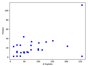
Figure 5: $\mathsf{Risk}$ calculation time for output of Fashion on pod $8$ instances using Python implementation of Frigault et al.’s algorithm [18].

We now ask if the algorithm of Frigault et al. [18] could be directly used in place of $\mathsf{Reach}$ and $\mathsf{Path}$. We created a Python implementation of this algorithm [14], analyzing instances of 128 hosts, with 12 to 250 vulnerabilities. Figure 5 shows the time required to compute the actual $\mathsf{Risk}$, with $\alpha=.7$ using our Python implementation of the algorithm by Frigault et al. [18] of one network configuration output by Fashion. Over this set of benchmarks, the computation time for the risk values of a single fixed configuration can reach 100 seconds for 250 exploits. Fashion inspects thousands of configurations during its search. The time to evaluate the risk seems correlated to the number of exploits, and the evaluation algorithms start to struggle even with a relatively small number (e.g., 50) exploits.

The search space associated with this kind of problem is generally huge. Directly specifying $\mathsf{Risk}$ would yield a highly non-linear, and thus likely intractable, formulation. Enumerating configurations and computing the risk a posteriori would be equally intractable. Linearization is therefore essential in a responsive and practical framework.

Incorporating Functionality

The paper demonstrates that Fashion can explore the trade-off between functionality and risk.

As stated, Fashion optimizes over both objectives but the model can easily be converted into one where either security or functionality is a constraint and the other objective is optimized. The average of $\mathsf{Path}$ and $\mathsf{Reach}$ is an effective linearizable stand in for a risk calculation that is prohibitively expensive to compute on the scale needed for a configuration search problem. Interestingly, the novel hybrid risk model enables Fashion to overcome their respective weaknesses and produce better solutions. Practically, Fashion runs in matter of minutes on networks of reasonable size (613 devices) and demonstrates potential for scalability. Finally, the empirical results indicate that the approximation adopted by Fashion does not jeopardize key properties such as monotonicity of functionality vs. risk.

The Fashion framework is a first step towards handling both functionality and risk for short-term response while producing consistent results with natural interpretations. Future directions include improving handling scalability of the model size that currently depends on the number of network links as well as the number of data flows and supporting a more varied set of controls beyond routing and blocking. Additional future work is understanding if there are network settings that require a different weighting of the two measures of $\mathsf{Path}$ and $\mathsf{Reach}$. Lastly, evaluation of Fashion configurations should continue using real data and real SDNs to understand emergent artifacts.

Other settings

Fashion’s primary application is quick response to new security information in an SDN. However, attack graph analyses are notoriously complex. Fashion’s security layer is useful for network planning as well. Fashion allows an organization to consider “what-if” queries for proposed changes in the network. One could consider the deployment of a new webserver on either Apache or Nginx (along with introduction of corresponding vulnerabilities) and understand how this would affect the overall risk posture of the network. Importantly, these analyses would consider this risk while maintaining network functional requirements. Once a small set of possible solutions has been identified, one can then validate Fashion’s output as described in the Introduction.

References

- [1] P. Kotzias, L. Bilge, P.-A. Vervier, and J. Caballero, “Mind your own business: A longitudinal study of threats and vulnerabilities in enterprises.” in NDSS, 2019.
- [2] G. Schryen, “Is open source security a myth? what do vulnerability and patch data say?” Communications of the ACM (CACM), vol. 54, no. 5, pp. 130–139, 2011.
- [3] N. Poolsappasit, R. Dewri, and I. Ray, “Dynamic security risk management using bayesian attack graphs,” IEEE Transactions on Dependable and Secure Computing, vol. 9, no. 1, pp. 61–74, 2011.
- [4] A. Lenin, O. Gadyatskaya, D. Ionita, W. Pieters, A. Tanner, S. Saraiva, C. Muller, J. Willemson, M. Ford, and S. Muller, “Technology-supported risk estimation by predictive assessment of socio-technical security,” 2016.
- [5] MITRE, “Common vulnerabilities and exposures,” https://cve.mitre.org, accessed 2020-01-15.
- [6] R. Dewri, N. Poolsappasit, I. Ray, and D. Whitley, “Optimal security hardening using multi-objective optimization on attack tree models of networks,” in Proceedings of the 14th ACM conference on Computer and communications security - CCS ’07. New York, New York, USA: ACM Press, 2007, p. 204. [Online]. Available: http://portal.acm.org/citation.cfm?doid=1315245.1315272
- [7] M. H. Khouzani, Z. Liu, and P. Malacaria, “Scalable min-max multi-objective cyber-security optimisation over probabilistic attack graphs,” European Journal of Operational Research, vol. 278, no. 3, pp. 894–903, 2019. [Online]. Available: https://doi.org/10.1016/j.ejor.2019.04.035
- [8] R. E. Sawilla and X. Ou, “Identifying critical attack assets in dependency attack graphs,” in European Symposium on Research in Computer Security. Springer, 2008, pp. 18–34.
- [9] K. Ingols, M. Chu, R. Lippmann, S. Webster, and S. Boyer, “Modeling modern network attacks and countermeasures using attack graphs,” in 2009 Annual Computer Security Applications Conference. IEEE, 2009, pp. 117–126.
- [10] H. Huang, S. Zhang, X. Ou, A. Prakash, and K. Sakallah, “Distilling critical attack graph surface iteratively through minimum-cost sat solving,” in Proceedings of the 27th Annual Computer Security Applications Conference. ACM, 2011, pp. 31–40.
- [11] Z. Aslanyan and F. Nielson, “Pareto efficient solutions of attack-defence trees,” in International Conference on Principles of Security and Trust. Springer, 2015, pp. 95–114.
- [12] W. Pieters, D. Hadziosmanovic, A. Lenin, L. Montoya, and J. Willemson, “Trespass: plug-and-play attacker profiles for security risk analysis,” IEEE Security & Privacy poster abstracts, 2014.
- [13] B. Kordy, L. Piètre-Cambacédès, and P. Schweitzer, “DAG-based attack and defense modeling: Don’t miss the forest for the attack trees,” 2014.
- [14] D. Callahan, T. Curry, H. Davidson, Z. T., B. Fuller, and L. Michel, “Functional and attack graph secured hybrid optimization of virtualized networks.” [Online]. Available: https://github.com/devoncal77/FASHION
- [15] N. Foster, R. Harrison, M. J. Freedman, C. Monsanto, J. Rexford, A. Story, and D. Walker, “Frenetic: A network programming language,” ACM Sigplan Notices, vol. 46, no. 9, pp. 279–291, 2011.
- [16] M. Boutier and J. Chroboczek, “Source-specific routing,” in 2015 IFIP Networking Conference (IFIP Networking). IEEE, 2015, pp. 1–9.
- [17] M. Al-Fares, A. Loukissas, and A. Vahdat, “A scalable, commodity data center network architecture,” in Proceedings of the ACM SIGCOMM 2008 Conference on Data Communication, ser. SIGCOMM ’08. New York, NY, USA: ACM, 2008, pp. 63–74. [Online]. Available: http://doi.acm.org/10.1145/1402958.1402967
- [18] M. Frigault, L. Wang, S. Jajodia, and A. Singhal, “Measuring the overall network security by combining cvss scores based on attack graphs and bayesian networks,” in Network Security Metrics. Springer, 2017, pp. 1–23.
- [19] M. Chu, K. Ingols, R. Lippmann, S. Webster, and S. Boyer, “Visualizing attack graphs, reachability, and trust relationships with navigator,” in Proceedings of the Seventh International Symposium on Visualization for Cyber Security, 2010, pp. 22–33.
- [20] M. U. Aksu, K. Bicakci, M. H. Dilek, A. M. Ozbayoglu et al., “Automated generation of attack graphs using NVD,” in Proceedings of the Eighth ACM Conference on Data and Application Security and Privacy, vol. 2018-Janua. ACM, 2018, pp. 135–142.
- [21] K. Piwowarski, “Evaluating and Strengthening Enterprise,” Network, no. October, 2005.
- [22] R. P. Lippmann and K. W. Ingols, “An annotated review of past papers on attack graphs,” Massachusetts Inst of Tech Lexington Lincoln Lab, Tech. Rep., 2005.
- [23] S. Bistarelli, F. Fioravanti, and P. Peretti, “Defense trees for economic evaluation of security investments,” Proc. - First Int. Conf. Availability, Reliab. Secur. ARES 2006, vol. 2006, pp. 416–423, 2006.
- [24] S. K. Fayaz, Y. Tobioka, V. Sekar, and M. Bailey, “Bohatei: Flexible and elastic ddos defense,” in 24th USENIX Security Symposium (USENIX Security 15), 2015, pp. 817–832.
- [25] J. Reich, C. Monsanto, N. Foster, J. Rexford, and D. Walker, “Modular SDN programming with Pyretic,” Technical Reprot of USENIX, 2013.
- [26] M. Reitblatt, N. Foster, J. Rexford, C. Schlesinger, and D. Walker, “Abstractions for network update,” ACM SIGCOMM Computer Communication Review, vol. 42, no. 4, pp. 323–334, 2012.
- [27] A. Khurshid, W. Zhou, M. Caesar, and P. Godfrey, “Veriflow: Verifying network-wide invariants in real time,” in Proceedings of the first workshop on Hot topics in software defined networks. ACM, 2012, pp. 49–54.
- [28] B. Schneier, “Attack trees,” Dr. Dobb’s journal, vol. 24, no. 12, pp. 21–29, 1999.
- [29] R. Yu, G. Xue, V. T. Kilari, and X. Zhang, “Deploying robust security in internet of things,” in IEEE Conference on Computer and Network Security, 2018.
- [30] R. Wang, D. Butnariu, J. Rexford et al., “Openflow-based server load balancing gone wild.” Hot-ICE, vol. 11, pp. 12–12, 2011.
- [31] R. Skowyra, A. Lapets, A. Bestavros, and A. Kfoury, “A verification platform for SDN-enabled applications,” in Cloud Engineering (IC2E), 2014 IEEE International Conference on. IEEE, 2014, pp. 337–342.
- [32] K. Subramanian, L. D’Antoni, and A. Akella, “Genesis: Synthesizing forwarding tables in multi-tenant networks,” in Conference Record of the Annual ACM Symposium on Principles of Programming Languages. Association for Computing Machinery, jan 2017, pp. 572–585.
- [33] A. El-Hassany, P. Tsankov, L. Vanbever, M. Vechev, and E. Zürich, “NetComplete: Practical Network-Wide Configuration Synthesis with Autocompletion,” Tech. Rep.
- [34] R. Majumdar and V. Kunčak, Eds., Computer Aided Verification, ser. Lecture Notes in Computer Science. Cham: Springer International Publishing, 2017, vol. 10427. [Online]. Available: http://link.springer.com/10.1007/978-3-319-63390-9
- [35] S. Narain, G. Levin, S. Malik, and V. Kaul, “Declarative infrastructure configuration synthesis and debugging,” in Journal of Network and Systems Management, vol. 16, no. 3, sep 2008, pp. 235–258.
- [36] R. Beckett, R. Mahajan, T. Millstein, J. Padhye, and D. Walker, “Don’t mind the gap: Bridging network-wide objectives and device-level configurations,” in SIGCOMM 2016 - Proceedings of the 2016 ACM Conference on Special Interest Group on Data Communication. Association for Computing Machinery, Inc, aug 2016, pp. 328–341.
- [37] T. Curry, D. Callahan, B. Fuller, and L. Michel, “DOCSDN: Dynamic and optimal configuration of software-defined networks,” in Australasian Conference on Information Security and Privacy. Springer, 2019, pp. 456–474.
- [38] M. Frigault and L. Wang, “Measuring network security using bayesian network-based attack graphs,” Proceedings - International Computer Software and Applications Conference, pp. 698–703, 2008.
- [39] R. Y. Chia, “SPAR: an autonomous SDN intrusion response framework using combinatorial optimization over a probabilistic attack graph,” Master’s thesis, Massachusetts Institute of Technology, 2020.
- [40] O. Sheyner, J. Haines, S. Jha, R. Lippmann, and J. M. Wing, “Automated generation and analysis of attack graphs,” in Security and privacy, 2002. Proceedings. 2002 IEEE Symposium on. IEEE, 2002, pp. 273–284.
- [41] K. Ingols, R. Lippmann, and K. Piwowarski, “Practical attack graph generation for network defense,” in Computer Security Applications Conference, 2006. ACSAC’06. 22nd Annual. IEEE, 2006, pp. 121–130.
- [42] P. Ammann, D. Wijesekera, and S. Kaushik, “Scalable, graph-based network vulnerability analysis,” in Proceedings of the 9th ACM Conference on Computer and Communicatio ns Security. ACM, 2002, pp. 217–224.
- [43] J. Homer, X. Ou, and D. Schmidt, “A sound and practical approach to quantifying security risk in enterprise networks,” Kansas State University Technical Report, pp. 1–15, 2009.
- [44] NIST, “Cybersecurity framework,” April 2018. [Online]. Available: https://www.nist.gov/cyberframework/framework
- [45] H. M. Almohri, L. T. Watson, D. Yao, and X. Ou, “Security optimization of dynamic networks with probabilistic graph modeling and linear programming,” IEEE Transactions on Dependable and Secure Computing, vol. 13, no. 4, pp. 474–487, 2016. [Online]. Available: http://www.ieee.org/publications_standards/publications/rights/index.html
- [46] NIST, “National vulnerability database,” = https://nvd.nist.gov, accessed 2020-01-10.
- [47] FIRST, “Common vulnerability scoring system,” June 2019. [Online]. Available: https://www.first.org/cvss/
- [48] MITRE, “Common weakness scoring system,” December 2018. [Online]. Available: https://cwe.mitre.org/cwss/cwss_v1.0.1.html/
- [49] J. Homer, S. Zhang, X. Ou, D. Schmidt, Y. Du, S. R. Rajagopalan, and A. Singhal, “Aggregating vulnerability metrics in enterprise networks using attack graphs,” Journal of Computer Security, vol. 21, no. 4, pp. 561–597, 2013.
- [50] A. Singhal and X. Ou, “Security risk analysis of enterprise networks using probabilistic attack graphs,” in Network Security Metrics. Springer, 2017, pp. 53–73.
- [51] R. W. Ritchey and P. Ammann, “Using model checking to analyze network vulnerabilities,” Proceedings of the IEEE Computer Society Symposium on Research in Security and Privacy, pp. 156–165, 2000.
- [52] Gurobi, “Gurobi software,” http://www.gurobi.com/.
- [53] C. Clos, “A Study of Non‐Blocking Switching Networks,” Bell System Technical Journal, 1953.
- [54] Cisco, “Cisco global cloud index 2016-21,” 2018.
- [55] M. Alizadeh, A. Greenberg, D. A. Maltz, J. Padhye, P. Patel, B. Prabhakar, S. Sengupta, and M. Sridharan, “Data Center TCP (DCTCP),” Computer Communication Review, vol. 40, no. 4, pp. 63–74, 2010.
- [56] Q. Zhou, K. Wang, P. Li, D. Zeng, S. Guo, B. Ye, and M. Guo, “Fast Coflow Scheduling via Traffic Compression and Stage Pipelining in Datacenter Networks,” IEEE Transactions on Computers, vol. PP, no. c, pp. 1–1, 2019.
- [57] T. Benson, A. Akella, and D. A. Maltz, “Network traffic characteristics of data centers in the wild,” in Proceedings of the 10th ACM SIGCOMM Conference on Internet Measurement, ser. IMC ’10. New York, NY, USA: ACM, 2010, pp. 267–280. [Online]. Available: http://doi.acm.org/10.1145/1879141.1879175
- [58] C. Delimitrou, S. Sankar, A. Kansal, and C. Kozyrakis, “ECHO: Recreating network traffic maps for datacenters with tens of thousands of servers,” Proceedings - 2012 IEEE International Symposium on Workload Characterization, IISWC 2012, pp. 14–24, 2012.
- [59] S. Kandula, “Inside the Social Network ’ s ( Datacenter ) Network – Public Review,” pp. 123–137.
- [60] S. Zhang, X. Zhang, and X. Ou, “After we knew it: empirical study and modeling of cost-effectiveness of exploiting prevalent known vulnerabilities across IaaS cloud,” in AsiaCCS – Proceedings of the 9th ACM symposium on Information, computer and communications security, 2014, pp. 317–328.
- [61] T. Ralphs and M. Güzelsoy, “Duality and warm starting in integer programming,” in The Proceedings of the 2006 NSF Design, Service, and Manufacturing Grantees and Research Conference, 2006.
- [62] S. M. Pour, J. H. Drake, L. S. Ejlertsen, K. M. Rasmussen, and E. K. Burke, “A hybrid constraint programming/mixed integer programming framework for the preventive signaling maintenance crew scheduling problem,” European Journal of Operational Research, vol. 269, no. 1, pp. 341 – 352, 2018. [Online]. Available: http://www.sciencedirect.com/science/article/pii/S0377221717307646