Identical pion intensity interferometry at $\boldmath{\sqrt{s_{\mathrm{NN}}}=}$2.4 GeV

Abstract

High-statistics $\pi^{-}\pi^{-}$ and $\pi^{+}\pi^{+}$ femtoscopy data are presented for Au + Au collisions at $\sqrt{s_{\mathrm{NN}}}=2.4$ GeV, measured with HADES at SIS18/GSI. The experimental correlation functions allow the determination of the space-time extent of the corresponding emission sources via a comparison to models. The emission source, parametrized as three-dimensional Gaussian distribution, is studied in dependence on pair transverse momentum, azimuthal emission angle with respect to the reaction plane, collision centrality and beam energy. For all centralities and transverse momenta, a geometrical distribution of ellipsoidal shape is found in the plane perpendicular to the beam direction with the larger extension perpendicular to the reaction plane. For large transverse momenta, the corresponding eccentricity approaches the initial eccentricity. The eccentricity is smallest for most central collisions, where the shape is almost circular. The magnitude of the tilt angle of the emission ellipsoid in the reaction plane decreases with increasing centrality and increasing transverse momentum. All source radii increase with centrality, largely exhibiting a linear rise with the cube root of the number of participants. A substantial charge-sign difference of the source radii is found, appearing most pronounced at low transverse momentum. The extracted source parameters are consistent with the extrapolation of their energy dependence down from higher energies.

1 Introduction

Two-particle intensity interferometry of hadrons is widely used to study the spatio-temporal size, shape and evolution of their source in heavy-ion collisions or other reactions involving hadrons (for a review see ref. Lisa05 ). The technique, pioneered by Hanbury Brown and Twiss HBT56 to measure angular radii of stars, later on named HBT interferometry, is based on the quantum-statistical interference of identical particles. Goldhaber et al. GGLP60 first applied intensity interferometry to hadrons. In heavy-ion collisions, the intensity interferometry does not allow to measure directly the reaction volume, as the emission zone, changing shape and size in the course of the collision, is affected by dynamically generated space-momentum correlations (e.g. radial expansion after the compression phase or resonance decays). Thus, intensity interferometry generally does not yield the proper source size, but rather an effective “length of homogeneity” Lisa05 . It measures source regions in which particle pairs are close in momentum, so that they are correlated as a consequence of their quantum statistics or due to their two-body interaction. At energies in the GeV region, the measured particles can originate from many different processes. Therefore, the intensity interferometry may provide additional information to the understanding of reaction mechanisms which finally determine the particle emission sources.

In general, the sign and strength of the correlation is affected by (i) the strong interaction, (ii) the Coulomb interaction if charged particles are involved, and (iii) the quantum statistics in the case of identical particles (Fermi-Dirac suppression for fermions, Bose-Einstein enhancement for bosons). In the case of $\pi\pi$ correlations, the mutual strong interaction appears to be negligible Bowler88 compared to the effects (ii) and (iii).

It is worth emphasizing that, before the measurement presented here, only preliminary data hbt_fopi_1995 of identical-pion HBT data exist for a large symmetric collision system (like Au + Au or Pb + Pb) at a beam kinetic energy of about $1\mbox{$A$~{}GeV}$ (fixed target, $\sqrt{s_{\mathrm{NN}}}=2.3$ GeV). For the somewhat smaller system La + La, studied at $1.2A$ GeV with the HISS spectrometer at the Lawrence Berkeley Laboratory (LBL) Bevalac, pion correlation data were reported by Christie et al. Christie93 ; Christie92 . An oblate shape of the pion source and a correlation of the source size with the system size were found. Also, pion intensity interferometry for small systems (Ar + KCl, Ne + NaF) was studied at 1.8$A$ GeV at the LBL Bevalac using the Janus spectrometer by Zajc et al. Zajc84 . Both groups made first attempts to correct the influence of the pion-nuclear Coulomb interaction on the pion momenta. The effect on the source radii, however, was found negligible for their experiments.

In this article we report on the investigation of $\pi^{-}\pi^{-}$ and $\pi^{+}\pi^{+}$ correlations at low relative momenta in Au + Au collisions at 1.23$A$ GeV  (fixed target, $p_{\mathrm{proj}}/A=1.96$ GeV$/c$, $\sqrt{s_{\mathrm{NN}}}=2.41$ GeV), continuing our previous femtoscopic studies of smaller collisions systems hades_pLambda_ArKCl ; hades_hbt_ArKCl ; hades_pLambda_pNb . In a recent letter hades_HBT_letter presenting only the results of the azimuthally-integrated HBT analysis for central collision, we reported a substantial charge-sign difference of the source radii, particularly pronounced at low transverse momenta, and a smooth extrapolation of the $\sqrt{s_{\mathrm{NN}}}$ dependence of the source parameters towards low energies. Here, we present the complete HBT analysis, including azimuthal-angle and centrality dependences. In Sect. 2 we shortly describe the experiment. In Sect. 3 we define the correlation function and discuss possible distortions to it. In Sect. 4 we present the three-dimensional pion emission source resulting from the correlation analysis, its dependences on collisions centrality and kinematic quantities and compare our observations to the findings of other experiments. Finally, we summarize our results in Sect. 5 and give an outlook.

2 The experiment

The measurement was performed with the High Acceptance Di-Electron Spectrometer (HADES) at the Schwerionensynchrotron SIS18 at GSI, Darmstadt. HADES, although primarily optimized to measure di-electrons HADES-PRL07 , offers also excellent hadron identification capabilities hades_kpm_phi_arkcl ; hades_xi_arkcl ; hades_K0_ArKCl ; hades_Lambda_ArKCl ; hades_xi_pNb ; hades_kpm_phi_auau . The setup of the HADES experiment is described in detail in Agakishiev:2009am . HADES is a charged particle detector consisting of a six-coil toroidal magnet centered around the beam axis and six identical detection sections located between the coils and covering polar angles between $18^{\circ}$ and $85^{\circ}$. Each sector is equipped with a Ring-Imaging Cherenkov (RICH) detector followed by four layers of Mini-Drift Chambers (MDCs), two in front of and two behind the magnetic field, as well as a scintillator Time-Of-Flight detector (TOF) ($44^{\circ}$ – $85^{\circ}$) and Resistive Plate Chambers (RPC) ($18^{\circ}$ – $45^{\circ}$). TOF, RPC, and Pre-Shower detectors (behind RPC, for e^± identification) were combined into a Multiplicity and Electron Trigger Array (META). Charged hadron identification is based on the time-of-flight measured with TOF and RPC, and on the energy-loss information from TOF as well as from the MDC tracking chambers. Electron candidates are in addition selected via their signals in the RICH detector. Combining this information with the momentum, $p$, as determined from the deflection of the tracks in the magnetic field, allows to identify charged particles (e.g. pions, kaons or protons) with a high significance. Particles are assumed to be identified as pions if their velocity, $\beta$, is found within a $3\sigma$ window around the theoretical expectation, $\beta_{\pi}=p/\sqrt{p^{2}+m_{\pi}^{2}}$. The corresponding cut parameters $\sigma$ are derived from Gaussian fits to the velocity distribution in slices of momentum. (We use units with $\hbar=c^{2}=1$.)

Several triggers are implemented. The minimum bias trigger is defined by a signal in a diamond START detector in front of the 15-fold segmented gold target. In addition, online Physics Triggers (PT) are used, which are based on hardware thresholds on the TOF signals, proportional to the event multiplicity, corresponding to at least 5 (PT2) or 20 (PT3) hits in the TOF. Events are selected offline by requiring that their global event vertex is inside the target region, i.e. within an interval of 65 mm along the beam axis. About 2.1 billion Au + Au collisions corresponding to the 43 % most central events are taken into account for the present correlation analysis.

The centrality determination is based on the summed number of hits detected by the TOF and the RPC detectors. The measured events are divided in centrality classes corresponding to intervals of the integrated cross section. Note that, as a result of the analogue hardware threshold of the online trigger, the most peripheral class can be extended to 45 % (or even further), i.e. beyond the above given effective value.

The respective average impact parameters and mean numbers of nucleons participating in the formation of the nuclear fireball, $\langle A_{\mathrm{part}}\rangle$, as deduced from extensive Monte-Carlo (MC) calculations hades_centrality:2018am ; PhobosGlauber2015 with the Glauber model Glauber:1955qq are summarized in table 1.

The determination of the reaction plane angle, $\phi_{\mathrm{RP}}$, is based on the measurement of the charged projectile spectator fragments (mostly $Z=1,\,2$) by their position, flight time and energy deposit. They are detected by a three square meter scintillator hodoscope 7 m downstream the target, consisting of 288 scintillator cells. It covers polar angles from 0.3 to 7.2 degrees. Due to the dispersion of the event plane a resolution correction needs to be applied (cf. Sect. 4.4).

Finally, we want to note that, as result of both the neutron excess of the collision system and the different detector acceptances of negatively and positively charged particles, about five to six times more $\pi^{-}\pi^{-}$ pairs than $\pi^{+}\pi^{+}$ pairs are measured.

Table 1: The mean number of participants (2nd column) and the average impact parameter (3rd column) calculated hades_centrality:2018am with Glauber MC simulations PhobosGlauber2015 for the centrality classes listed in the 1st column. The 4th and 5th columns give the corresponding 1st and 2nd order reaction plane resolutions (cf. Sect. 4.4), respectively, calculated according to ref. Ollitrault97 .

Centrality	$\langle A_{\mathrm{part}}\rangle$	$\langle b\rangle$	$F_{1}$	$F_{2}$
($\%$)		(fm)
0$0\,-\,10$	$303$	$3.1$	0.648	0.298
$10\,-\,20$	$213$	$5.7$	0.847	0.572
$20\,-\,30$	$150$	$7.4$	0.887	0.653
$25\,-\,35$	$125$	$8.1$	0.886	0.651
$30\,-\,40$	$103$	$8.7$	0.876	0.629
$30\,-\,45$	$~{}93$	$9.0$	0.871	0.620

3 The correlation function

Generally, the two-particle correlation function is defined as the ratio of the probability $P_{2}({\bm{p}}_{1},{\bm{p}}_{2})$ to measure simultaneously two particles with momenta ${\bm{p}}_{1}$ and ${\bm{p}}_{2}$ and the product of the corresponding single-particle probabilities $P_{1}({\bm{p}}_{1})$ and $P_{1}({\bm{p}}_{2})$ Lisa05 ,

$$C({\bm{p}}_{1},{\bm{p}}_{2})=\frac{P_{2}({\bm{p}}_{1},{\bm{p}}_{2})}{P_{1}({\bm{p}}_{1})P_{1}({\bm{p}}_{2})}.$$ (1)

Experimentally this correlation is formed as a function of the momentum difference between the two particles of a given pair and quantified by taking the ratio of the yields of ’true’ pairs ($Y_{\mathrm{true}}$) and uncorrelated pairs ($Y_{\mathrm{mix}}$). $Y_{\mathrm{true}}$ is constructed from all particle pairs in the selected phase space interval from the same event. $Y_{\mathrm{mix}}$ is generated by event mixing, where particle 1 and particle 2 are taken from different events. Care was taken to mix particles from similar event classes in terms of multiplicity, vertex position and reaction plane angle. The events are allowed to differ by not more than 10 in the number of the RPC + TOF hit multiplicity (i.e. corresponding to the typical multiplicity uncertainty as deduced from simulations for fixed impact parameter hades_centrality:2018am ), 1.2 mm in the $z$-vertex coordinate (amounting to less than one third of the spacing between target segments), and 10 degrees in azimuthal angle relative to the reaction plane (significantly below the event plane resolution, cf. table 1), respectively. The momentum difference is decomposed into three orthogonal components as suggested by Podgoretsky Podgoretsky83 , Pratt Pratt86 and Bertsch Bertsch89 . The three-dimensional correlation functions are projections of Eq. (1) into the (out, side, long)-coordinate system, where ‘out’ means along the pair transverse momentum, ${\bm{p}}_{\mathrm{t,\,12}}={\bm{p}}_{\mathrm{t,\,1}}+{\bm{p}}_{\mathrm{t,\,2}}$, ‘long’ is parallel to the beam direction $z$, and ‘side’ is oriented perpendicular to the other two directions. The particles forming a pair are boosted into the longitudinally comoving system, where the $z$-components of the momenta cancel each other, $p_{z_{1}}+p_{z_{2}}=0$. This system choice allows for an adequate comparison with correlation data taken at very different, usually much higher, collision energies, where the distribution of the rapidity, $y=\tanh^{-1}{(\beta_{\mathrm{z}})}$, of produced particles is found to be not as narrow as in the present case but largely elongated. (Here, $\beta_{\mathrm{z}}=p_{\mathrm{z}}/E$, $E=\sqrt{p^{2}+m_{0}^{2}}$ and $m_{0}$ are the longitudinal velocity, the total energy and the rest mass of the particle, respectively. ) Hence, the experimental correlation function is given by

$$C(q_{\mbox{{\scriptsize out}}},q_{\mbox{{\scriptsize side}}},q_{\mbox{{\scriptsize long}}})={\cal N}\,\frac{Y_{\mathrm{true}}(q_{\mbox{{\scriptsize out}}},q_{\mbox{{\scriptsize side}}},q_{\mbox{{\scriptsize long}}})}{Y_{\mathrm{mix}}(q_{\mbox{{\scriptsize out}}},q_{\mbox{{\scriptsize side}}},q_{\mbox{{\scriptsize long}}})},$$ (2)

where $q_{i}=(p_{\mathrm{1,\,i}}-p_{\mathrm{2,\,i}})/2$ ($i$ = ’out’, ’side’, ’long’) are the relative momentum components, and ${\cal N}$ is a normalization factor which is fixed by the requirement $C\rightarrow 1$ at large relative momenta, where the correlation function is expected to flatten out at unity. The statistical errors of $C$ are dominated by those of the true yield, since the mixed yield is generated with much higher statistics. Analogously to Eq. (2), the experimental one-dimensional correlation function,

$$C(q_{\mbox{{\scriptsize inv}}})={\cal N}^{\prime}\,\frac{Y_{\mathrm{true}}(q_{\mbox{{\scriptsize inv}}})}{Y_{\mathrm{mix}}(q_{\mbox{{\scriptsize inv}}})},$$ (3)

is generated by projecting Eq. (1) onto the Lorentz-invariant relative momentum,

$$q_{\mbox{{\scriptsize inv}}}=\frac{1}{2}\sqrt{({\bm{p}}_{1}-{\bm{p}}_{2})^{2}-(E_{1}-E_{2})^{2}},$$ (4)

where $E_{i}=\sqrt{p^{2}_{i}+m^{2}_{i}}$ and $m_{i}$ ($i=1,\,2$) are the total energies and the rest masses of the particles forming the pair, respectively. Note that for two particles of equal mass, $q_{\mbox{{\scriptsize inv}}}$ is identical in magnitude to the single particle momenta in the rest frame of the pair.

3.1 Treatment of close-track effects

Two different methods to correct for the possible bias due to close-track effects introduced by the limitations of the HADES detector + track finding procedures are investigated and found to agree within statistical fluctuations.

Method A, called double-ratio method, is based on UrQMD UrQMD transport model simulations of Au + Au collisions at 1.23$A$ GeV fully transported through the HADES implementation HGeant of the ’Detector Description and Simulation Tool’ GEANT3.21 GEANT . Since UrQMD does not incorporate quantum-statistical or Coulomb effects, any identical-pion correlation function generated from the corresponding HGeant output according to Eq. (3) is expected to be flat at unity. Deviations from that value are considered to result from close-track effects. Hence, dividing the experimental and the simulated correlation functions should allow for a reasonable correction of the former one. However, this method is statistically limited because of the present availability to us of only 100 million UrQMD events, i.e. 20 times less than the experimental data sample. Thus, the statistical errors of the corrected correlation function would be dominated by those of the simulation, a drawback becoming particularly important when investigating the correlation function in a multi-dimensional parameter space. Also, it could not be fully guaranteed that HGeant is realistic enough in reproducing the behaviour of nearby tracks. These simulations also showed that there are no significant long-range correlations, usually attributed either to energy-momentum conservation in correlation analyses of small systems or to minijet-like phenomena at high energies. Therefore, this method serves for cross checks but is not involved in the results presented in Sect. 4.

Method B implements appropriate selection conditions on the META-hit and MDC-layer level, i.e. by discarding pairs which hit the same META cell, and by excluding for particle 2 three successive wires symmetrically around the MDC wire fired by particle 1. This method was tested with simulations based on UrQMD + HGeant and a detailed description of the detector response, to firmly exclude any close-track effect. Also broader exclusion windows have been investigated, but no significant improvement was found. Though there is a certain amount of pairs with small relative momenta getting lost due to this condition (about $50\,\%$ for $q_{\mbox{{\scriptsize inv}}}<40~{}\mbox{MeV$/c$}$), its superior statistical significance still clearly favors this method over the double-ratio method. Consequently, Method B, applied to both the true and the mixed-event yields, is used throughout the analysis RG presented in this article.

3.2 Parameterization of one-dimensional correlation functions

The fits to the one-dimensional correlation function are performed with the function

$$C(q_{\mbox{{\scriptsize inv}}})=N\left[1-\lambda_{\mbox{{\scriptsize inv}}}+\lambda_{\mbox{{\scriptsize inv}}}K_{\mathrm{C}}(q_{\mbox{{\scriptsize inv}}},R_{\mbox{{\scriptsize inv}}})C_{\mathrm{qs}}(q_{\mbox{{\scriptsize inv}}})\right],$$ (5)

using a Gaussian function for the quantum-statistical (Bose-Einstein) part,

$$C_{\mathrm{qs}}(q_{\mbox{{\scriptsize inv}}})=1+\exp{(-(2q_{\mbox{{\scriptsize inv}}}R_{\mbox{{\scriptsize inv}}})^{2})}.$$ (6)

The influence of the mutual Coulomb interaction in Eq. (5) is separated from the Bose-Einstein part by including in the fits the commonly used Coulomb correction by Sinyukov et al. Sinyukov98 . The Coulomb factor $K_{\mathrm{C}}$ results from the integration of the two-pion Coulomb wave function squared over a spherical Gaussian source of fixed radius. This radius is iteratively approximated by the result of the corresponding fit to the correlation function. The parameters $N$ and $\lambda$ in Eq. (5) represent a normalization constant and the fraction of correlated pairs, respectively.

All fits performed to one-dimensional and three-dimensional (cf. Sect. 3.3) correlation functions involve a log-likelihood minimization Ahle02 . No significant differences are observed when using a $\chi^{2}$ minimization.

3.3 Parameterization of three-dimensional correlation functions

The three-dimensional experimental correlation function is fitted with the function

$$C(q_{\mbox{{\scriptsize out}}},\,q_{\mbox{{\scriptsize side}}},\,q_{\mbox{{\scriptsize long}}})=$$

$$N\big{[}1-\lambda_{\mbox{{\scriptsize osl}}}+\lambda_{\mbox{{\scriptsize osl}}}K_{\mathrm{C}}(\hat{q},R_{\mbox{{\scriptsize inv}}})C_{\mathrm{qs}}(q_{\mbox{{\scriptsize out}}},\,q_{\mbox{{\scriptsize side}}},\,q_{\mbox{{\scriptsize long}}})\big{]},$$ (7)

where, for azimuthally-integrated analyses (Sect. 4.3) at midrapidity ($y_{\mathrm{cm}}=0.74$),

$$C_{\mathrm{qs}}(q_{\mbox{{\scriptsize out}}},\,q_{\mbox{{\scriptsize side}}},\,q_{\mbox{{\scriptsize long}}})=$$

$$1+\exp{(-(2q_{\mbox{{\scriptsize out}}}R_{\mbox{{\scriptsize out}}})^{2}-(2q_{\mbox{{\scriptsize side}}}R_{\mbox{{\scriptsize side}}})^{2}-(2q_{\mbox{{\scriptsize long}}}R_{\mbox{{\scriptsize long}}})^{2})}\hfill$$ (8)

represents the quantum-statistical part of the correlation function and

$$\hat{q}=q_{\mbox{{\scriptsize inv}}}(q_{\mbox{{\scriptsize out}}},\,q_{\mbox{{\scriptsize side}}},\,q_{\mbox{{\scriptsize long}}},\bar{k}_{\mathrm{t}})$$ (9)

is the average value of the invariant momentum difference for given intervals of the relative momentum components and $k_{\mathrm{t}}$. Actually, Eq. (8) can be written in a more general way,

$$C_{\mathrm{qs}}=1+\exp{(-4\sum_{i,\,j}q_{i}R^{2}_{ij}q_{j})},$$ (10)

as used for the azimuthally-sensitive HBT analyses presented in Sect. 4.4. For symmetry reasons UHeinz02 the non-diagonal ($i\neq j$) elements of $R_{ij}$, comprising the combinations ’out’-’side’ and ’side’-’long’, vanish when azimuthally and rapidity integrated analyses are performed e895_2000 ; HBT_in_UrQMD , as is done in Sect. 4.3. The ’out’-’long’ component, however, should have a finite value depending on the degree of symmetry of the detector-accepted rapidity distribution w.r.t. midrapidity. We studied this effect by including in Eq. (8) an additional term $-2q_{\mbox{{\scriptsize out}}}(2R_{\mbox{{\scriptsize out\,long}}})^{2}q_{\mbox{{\scriptsize long}}}$, where the prefactor accounts for both non-diagonal terms, ’out-long’ and ’long-out’. We found only marginal differences in the fits which resulted, for all centrality and transverse-momentum classes, in rather small values of $R^{2}_{\mathrm{out\,long}}<1$ fm², which in many cases are consistent with zero within uncertainties. This finding is not surprising, since the rapidity distribution of charged pions accepted by HADES is almost centered at midrapidity and rather narrow, i.e. extending just over about $\pm 0.7$ rapidity units.

Finally, for all results presented in Sect. 4, we restricted the pair rapidity to an interval $|y-y_{\mathrm{cm}}|<0.35$, within which $dN/dy$ does not vary by more than 10 %.

3.4 Momentum resolution correction

The effect of the finite momentum resolution of the HADES tracking system Agakishiev:2009am is studied with dedicated simulations. For that purpose, pairs of identical pions (resulting from the two-body decay of a fictive mother particle with its mass chosen to produce relative momenta of interest, e.g. $q_{\mbox{{\scriptsize inv}}}=10,\,20,\,30,\,...~{}\mbox{MeV$/c$}$) are simulated with the event generator Pluto Pluto and subsequently tracked through HGeant, the latter one modelling the HADES detector with its granularity and momentum resolution. The relative-momentum distribution of the pion pairs delivered by the simulation is fitted with a Gaussian function. The resulting widths $\sigma_{q}(q_{\mathrm{i}})$ (i=’inv’, ’out’, ’side’, ’long’) are folded into the fit functions (Eqs. (5) and (7)) to account for the slight resolution-induced decrease of both $R$ and $\lambda$. A typical resolution amounts to $\sigma_{q}(q_{\mbox{{\scriptsize inv}}}=20~{}\mbox{MeV$/c$})\simeq 2~{}\mbox{MeV$/c$}$ corresponding to a radius shift of $\Delta R/R\simeq+2$ % after the correction.

3.5 Systematic error estimate

The main contribution to the systematic uncertainties of the results presented in the subsequent section is due to the fluctuation of the fit results when varying the fit range over the respective relative-momentum quantity. The standard fit range was chosen to an interval extending from 4 to $80~{}\mbox{MeV$/c$}$. We varied the lower limit to $8~{}\mbox{MeV$/c$}$ and the upper one from 60 to $100~{}\mbox{MeV$/c$}$. Typical radius changes of $0.1-0.3$ fm are observed.

The contribution of the close-track effects discussed in Sect. 3.1 was estimated by varying the size of the wire-exclusion window (3 vs. 5 wires) in Method B. The resulting radius uncertainties did not exceed 0.2 fm; typically they were smaller than 0.1 fm.

The influence of possible impurities entering the charged pion samples was tested with stronger cuts on the quality parameters of particle identification (cf. Sect. 2), i.e. by a $\pm 30~{}\mbox{MeV}$ mass window around the most probable pion mass. About two third of the pairs survived this cut. No systematic differences w.r.t. to the full data sample are found within the statistical errors.

The effect of varying $R_{\mathrm{inv}}$ in the Coulomb correction in Eq. (7) results in systematic uncertainties of $\sim 0.01$  fm; the effect of the finite size of the averaging intervals in Eq. (9) yields systematic uncertainties of even smaller size.

The uncertainty of the momentum resolution correction described in Sect. 3.4 appears to be an order of magnitude smaller than the absolute source radius shift, i.e. typical values of $0.01-0.03$ fm are considered.

Another systematic uncertainty was estimated from studies of the forward-backward symmetry of the fit results w.r.t. midrapidity. Selecting the rapidity windows $-0.35<y-y_{\mathrm{cm}}<0$ and $0<y-y_{\mathrm{cm}}<0.35$ and taking similar (unbiased by the detector acceptance) transverse momentum intervals, typical systematic variations of the fit radii of $0.03-0.1$ (0.2) fm for $R_{\mathrm{inv}}$, $R_{\mathrm{side}}$, $R_{\mathrm{long}}$ ($R_{\mathrm{out}}$) are observed.

For the fit of the azimuthally integrated three-dimensional correlation function, the slight differences of the results when switching on/off the ’out’-’long’ component in the fit function (cf. Sect. 3.3) are taken as further systematic uncertainty. Typical values of these differences are $0.03-0.15$ fm.

As an additional cross check, the stability of the results w.r.t. a reversed setting (for about 10 % of the beam time) of the magnetic field has been investigated. Within the larger statistical errors, the results for $\pi^{-}\pi^{-}$ ($\pi^{+}\pi^{+}$) in reversed field are found identical to the $\pi^{-}\pi^{-}$ ($\pi^{+}\pi^{+}$) results in default field, although oppositely charged pions are subjected to different overall detector acceptances.

Finally, all systematic error contributions are added quadratically.

4 Results

4.1 Experimental correlation functions

The data are divided into centrality classes (cf. Sect. 2) and into classes of pair transverse momentum, $p_{\mathrm{t,\,12}}$, from which the pair transverse mass, $m_{\mathrm{t}}=\sqrt{k_{\mathrm{t}}^{2}+m_{\pi}^{2}}$ with $k_{t}=p_{\mathrm{t,\,12}}/2$, is derived. As width of the underlying $p_{\mathrm{t,\,12}}$ bins 100 MeV$/c$ was selected. In case of azimuthally-sensitive HBT analyses (Sect. 4.4), the bin size of the pair angle w.r.t. the reaction plane, $\Phi=\phi_{12}-\phi_{\mathrm{RP}}$, is chosen to be $\pi/4$.

A representative one-dimensional $\pi^{-}\pi^{-}$ correlation function fitted with Eq. (5) is shown in Fig. 1. Note that we usually exclude from the fits pairs with $q_{\mbox{{\scriptsize inv}}}<6~{}\mbox{MeV$/c$}$, since at very small relative momenta slight remnants of close-track effects could not completely be avoided when applying the correction Method B described in Sect. 3.1. This exclusion from the fit also renders a potential correction of the center of gravity of the first $q_{\mbox{{\scriptsize inv}}}$ bin unnecessary, within which the Coulomb factor $K_{\mathrm{C}}(q_{\mbox{{\scriptsize inv}}})$ exhibits a rather steep increase. (However, already within the 2nd bin function $K_{\mathrm{C}}$ is fairly smooth. Moreover, since both the true and mixed yields naturally show different slopes at low $q_{\mbox{{\scriptsize inv}}}$, a unique positioning of the corresponding bin centers required by Eq. (3) would be quite sophisticated.) For the quality of the three-dimensional fits we refer to hades_HBT_letter .

Two-dimensional projections of the Coulomb-corrected three-dimensional correlation function (Eq. (7)) are presented in Fig. 2 for $|\Phi|<\pi/8$. The low-momentum enhancement due to the quantum-statistical (Bose-Einstein) effect is visible in all three directions. Comparing these in-plane correlations with the corresponding out-of-plane ($|\Phi-\pi/2|<\pi/8$) correlations displayed in Fig. 3, a modification of the $q$ range of the Bose-Einstein part of the correlation becomes visible. (Due to the permutability of particles 1 and 2, one of the $q$ projections can be restricted to positive values.) Detailed results of the azimuthally-dependent correlation functions are presented in Sect. 4.4.

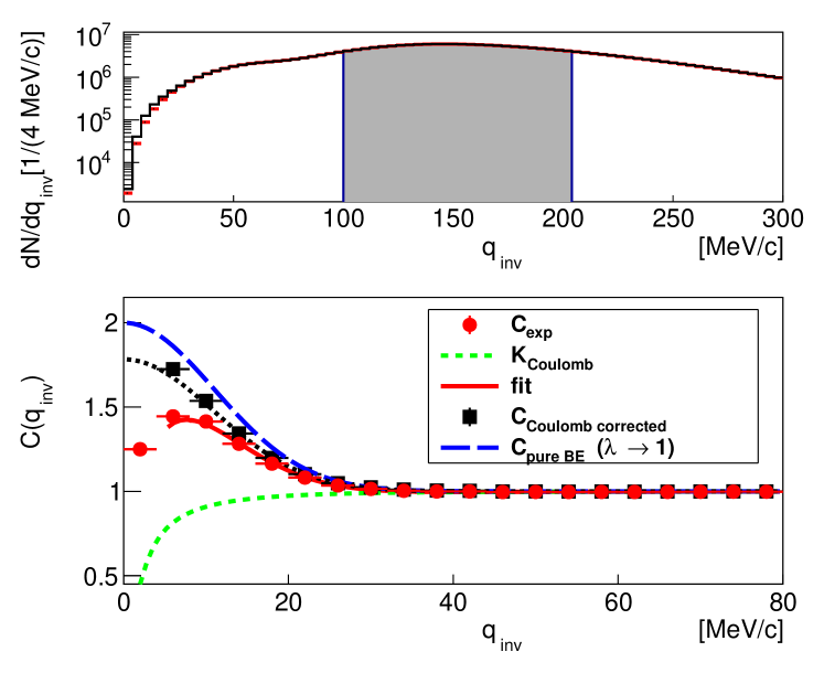
Figure 1: Upper panel: The distribution of the invariant relative momentum $q_{\mbox{{\scriptsize inv}}}$ for $\pi^{-}\pi^{-}$ pairs with transverse momentum of $p_{\mathrm{t,\,12}}=100-200~{}\mbox{MeV$/c$}$ for central ($0-10\,\%$) Au + Au collisions at 1.23$A$ GeV. The black (red) histogram displays the true (mixed) yield. The grey-shaded area represents the yield used for normalization. Lower panel: The one-dimensional $\pi^{-}\pi^{-}$ correlation function as function of $q_{\mbox{{\scriptsize inv}}}$. Red circles display the ratio of the true and mixed distributions, respectively. The green dashed curve represents the Coulomb correction function $K_{C}$ as described in Sect. 3.2. The black squares correspond to the Coulomb-corrected correlation function. The red full (black dotted) curve shows the fit function (Eq. (5)) before (after) the Coulomb correction. The blue long-dashed curve gives the pure Bose-Einstein part (Eq. (6)) of the correlation function.

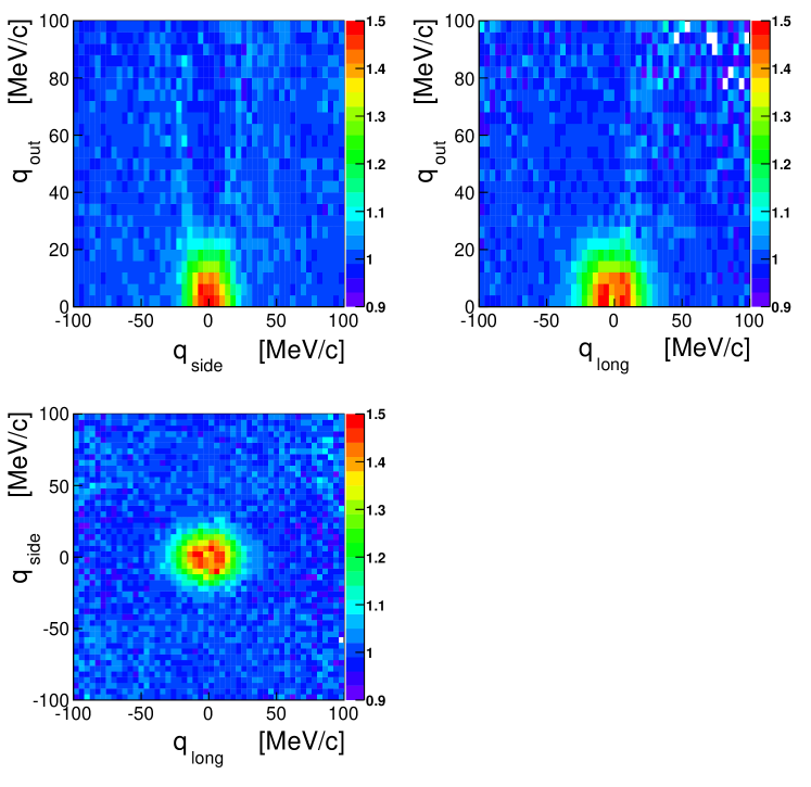
Figure 2: Two-dimensional projections of the Coulomb-corrected three-dimensional correlation function (Eq. (7)) in the ’out’ vs. ’side’ (upper left panel), ’out’ vs. ’long’ (upper right), and ’side’ vs. ’long’ (lower left) planes, respectively, for $\pi^{-}\pi^{-}$ pairs with transverse momentum of $p_{\mathrm{t,\,12}}=100-400~{}\mbox{MeV$/c$}$ and angles w.r.t. the reaction plane of $|\phi_{12}-\phi_{\mathrm{RP}}|<\pi/8$ for centralities of $10-30\,\%$. The respective third direction is integrated over $\pm 20~{}\mbox{MeV$/c$}$.

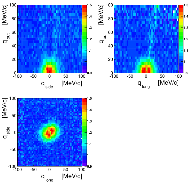
Figure 3: The same as Fig. 2, but for $|\phi_{12}-\phi_{\mathrm{RP}}-\pi/2|<\pi/8$.

4.2 Separation of central charge bias - construction of neutral pion radii

To quantify a potential source radius bias introduced by the Coulomb force the charged pions experience in the field of the charged fireball, we follow the ansatz used in ref. Baym_1996 ; Baym_1997 ,

$$E({\bm{p}}_{\mathrm{f}})=E({\bm{p}}_{\mathrm{i}})\pm V_{\mathrm{eff}}({\bm{r}}_{\mathrm{i}}),$$ (11)

where ${\bm{p}}_{\mathrm{i}}$ (${\bm{p}}_{\mathrm{f}}$) is the initial (final) momentum, $E$ the corresponding total energy, and ${\bm{r}}_{\mathrm{i}}$ the inital position of the pion in the Coulomb potential $V_{\mathrm{eff}}$ with positive (negative) sign for $\pi^{+}$ ($\pi^{-}$). With

$$\frac{R_{\pi^{\pm}\pi^{\pm}}}{R_{\pi^{0}\pi^{0}}}\approx\frac{q_{\mathrm{i}}}{q_{\mathrm{f}}} =\frac{|{\bm{p}}_{\mathrm{i}}|}{|{\bm{p}}_{\mathrm{f}}|}$$

$$=\sqrt{1\mp 2\frac{V_{\mathrm{eff}}}{|{\bm{p}}_{\mathrm{f}}|}\sqrt{1+\frac{m_{\pi}^{2}}{{\bm{p}}_{\mathrm{f}}^{2}}}+\frac{V^{2}_{\mathrm{eff}}}{{\bm{p}}_{\mathrm{f}}^{2}}},$$ (12)

where $q_{\mathrm{i}}$ ($q_{\mathrm{f}})$ is the initial (final) relative momentum, and with $V_{\mathrm{eff}}/k_{\mathrm{t}}\ll 1$, it turns out that the squared source radius for pairs of constructed neutral pions (denoted by $\tilde{\pi}^{0}\tilde{\pi}^{0}$ in the following) is simply the arithmetic mean of the corresponding quantities of the charged pions,

$$R_{\tilde{\pi}^{0}\tilde{\pi}^{0}}^{2}=\frac{1}{2}\big{(}R_{\pi^{+}\pi^{+}}^{2}+R_{\pi^{-}\pi^{-}}^{2}\big{)}.$$ (13)

Finally, the constructed $\tilde{\pi}^{0}\tilde{\pi}^{0}$ correlation radii, discussed in the subsequent sections, are derived from cubic spline interpolations of the $k_{\mathrm{t}}$ and $A_{\mathrm{part}}$ dependences of the corresponding experimental $\pi^{-}\pi^{-}$ and $\pi^{+}\pi^{+}$ data.

4.3 Azimuthally-integrated HBT analysis

4.3.1 Central collisions

We start with the study of source radii for central ($0-10\,\%$) collisions. Figure 4 shows the $m_{\mathrm{t}}$ dependence of the one-dimensional (invariant) and three-dimensional source radii for $\pi^{-}\pi^{-}$ (black squares) and $\pi^{+}\pi^{+}$ (red circles) pairs. While for low transverse mass the Coulomb interaction with the fireball leads to an increase (a decrease) of the source size derived for negative (positive) pion pairs, at large transverse momentum the Coulomb effect apparently fades away. The effect is smallest for $R_{\mbox{{\scriptsize out}}}$ and most pronounced for $R_{\mbox{{\scriptsize side}}}$. Note that the charge splitting of the source radii as well as its difference in magnitude in out and side direction was early on predicted by Barz Barz96 ; Barz99 who investigated the combined effects of nuclear Coulomb field, radial flow, and opaqueness on two-pion correlations for a large collision system such as Au + Au in the $1\mbox{$A$~{}GeV}$ energy regime. Earlier experimental works at the Bevalac employing a three-body Coulomb correction found the effect negligible for their studies of smaller systems Zajc84 ; Christie92 ; Christie93 . We note that the extent of the source in direction of ${\bm{k}}_{\mathrm{t}}$ is potentially enlarged by a finite emission time duration, which is expected to last a few fm /$c$ Lisa05 , cf. Sect. 4.4. It would be very interesting to study the charge-sign effect quantitatively with the help of dynamical models of the collision evolution. At present, such theoretical investigations concentrate on the higher energies where the charge splitting is hardly visible.

The parameter $\lambda_{\mbox{{\scriptsize osl}}}$ derived from the fits with Eq. (7) appears to be rather independent of transverse mass and charge sign and decreases only slightly with increasing transverse mass, cf. lower right panel of Fig. 4. It fits well into a preliminary evolution with $\sqrt{s_{\mathrm{NN}}}$ established previously STAR2015 , except the lowest E895 data point at 2$A$ GeV. In contrast, $\lambda_{\mbox{{\scriptsize inv}}}$ resulting from the fits to the one-dimensional correlation function, exhibits a significant decrease with $m_{\mathrm{t}}$ (cf. lower left panel), probably pointing to the fact that the one-dimensional fit function is not adequate.

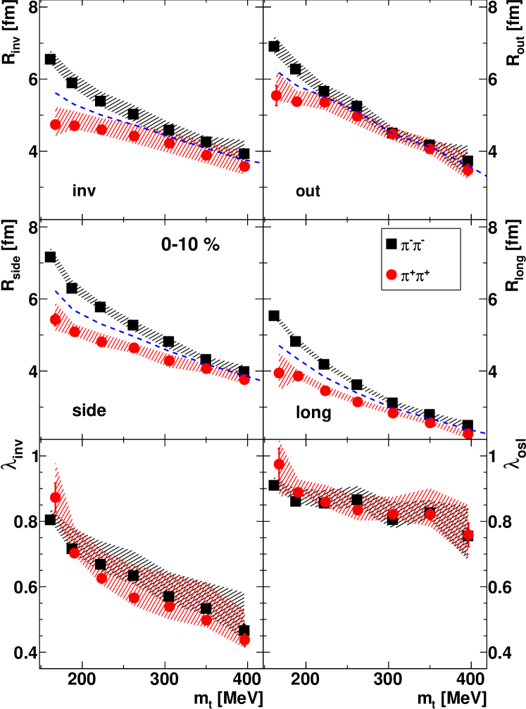
Figure 4: Source radii as function of pair transverse mass, $m_{\mathrm{t}}$, for central ($0-10\,\%$) Au + Au collisions at 1.23$A$ GeV. The corresponding $p_{\mathrm{t,\,12}}$ range amounts to $100-800~{}\mbox{MeV$/c$}$. The upper left, upper right, center left, and center right panels display the invariant, ’out’, ’side’, and ’long’ radii, respectively. The lower left and lower right panels show the corresponding $\lambda$ parameters resulting from the fits to the one- and three-dimensional correlation functions, respectively. Black squares (red circles) are for pairs of negative (positive) pions. Blue dashed curves represent constructed radii (Eq. (13)) of neutral pion pairs. Error bars and hatched bands represent the statistical and systematic errors, respectively.

4.3.2 Centrality dependence

Figure 5 exhibits the $A_{\mathrm{part}}$ dependence of source radii of $\pi^{-}\pi^{-}$ pairs (upper left panel) for the transverse-momentum interval $p_{\mathrm{t,\,12}}=300-400~{}\mbox{MeV$/c$}$. The volume of the overlap region (i.e. the participant zone) of the colliding nuclei is expected to be proportional to $A_{\mathrm{part}}$. Consequently, the involved length scales should be proportional to $A_{\mathrm{part}}^{1/3}$, which therefore could provide a good scaling variable for emission source radii. Close to linear dependences of the pion source radii as function of $A_{\mathrm{part}}^{1/3}$ are observed, as demonstrated by the straight-line fits to the data. The upper right panel of Fig. 5 shows the same for $\pi^{+}\pi^{+}$ source radii, following similar linear dependences on $A_{\mathrm{part}}^{1/3}$. Note that the $R_{\mbox{{\scriptsize inv}}}(A_{\mathrm{part}})$ dependences (black dotted lines) of the charged pion pairs, when extrapolated down to the $A_{\mathrm{part}}$ value (not shown) of the system Ar + KCl previously investigated by HADES hades_hbt_ArKCl , match the corresponding radii within uncertainties. This observation supports the idea that the variation of the participant volume via both, the choice of the size of the collision partners and the selection of a certain collision centrality, is equivalent. Following the recipe given in Sect. 4.2 to remove the Coulomb effect from the above dependences of $\pi^{-}\pi^{-}$ and $\pi^{+}\pi^{+}$ radii, we present the $A_{\mathrm{part}}^{1/3}$ dependence of constructed $\tilde{\pi}^{0}\tilde{\pi}^{0}$ source radii in the lower left panel of Fig. 5.

All results of the azimuthally integrated one-dimensional $(R_{\mbox{{\scriptsize inv}}},\,\lambda_{\mbox{{\scriptsize inv}}})$ and three-dimensional $(R_{\mbox{{\scriptsize out}}},\,R_{\mbox{{\scriptsize side}}},\,R_{\mbox{{\scriptsize long}}},\,\lambda_{\mbox{{\scriptsize osl}}})$ fits in dependence on collisions centrality and mean transverse momentum for $\pi^{-}\pi^{-}$, $\pi^{+}\pi^{+}$ and constructed $\tilde{\pi}^{0}\tilde{\pi}^{0}$ pairs are summarized in tables 2, 3 and 4, respectively.

Finally, the transverse-mass dependences of constructed $\tilde{\pi}^{0}\tilde{\pi}^{0}$ radii for different centrality classes are summarized in Fig. 6. The data are fitted (dashed curves) with a function

$$R=R_{0}\left(\frac{m_{\mathrm{t}}}{m_{\pi}}\right)^{\alpha}.$$ (14)

The fit parameters, $R_{0}=R(k_{\mathrm{t}}=0)$ and $\alpha$, derived from the $\chi^{2}$ minimizations are summarized in table 5. Here we emphasize that, while $\alpha$ derived from a fit to $R_{\mbox{{\scriptsize side}}}(m_{\mathrm{t}})$ of $\tilde{\pi}^{0}\tilde{\pi}^{0}$ follows the expectation (i.e. $\alpha=-0.5$) of (3+1)D hydrodynamics Kisiel2014 , its absolute value is larger (smaller) by $\sim 0.1$ when fitting the corresponding dependences of $\pi^{-}\pi^{-}$ ($\pi^{+}\pi^{+}$).

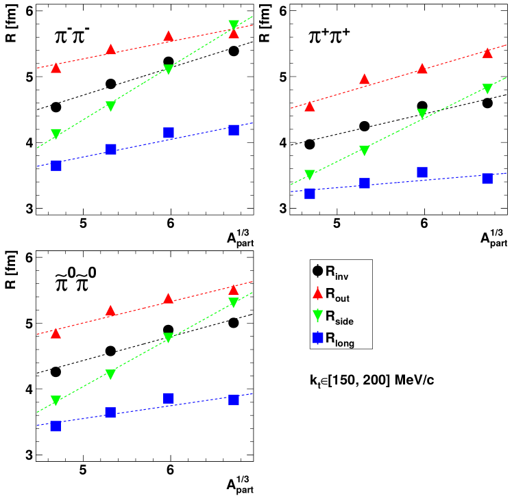
Figure 5: Source radii as function of the cube root of the number of participants for $\pi^{-}\pi^{-}$ (upper left) and $\pi^{+}\pi^{+}$ (upper right) pairs with transverse momenta of $p_{\mathrm{t,\,12}}=300-400~{}\mbox{MeV$/c$}$. The lower left panel shows corresponding radii of constructed neutral pions as deduced from interpolation of the charged-pion data according to the procedure decribed in Sect. 4.2. Black circles, red triangles, green inverted triangles, and blue squares display the ’invariant’, ’out’, ’side’, and ’long’ radii, respectively. Dotted lines represent $\chi^{2}$ fits to the data with straight lines.

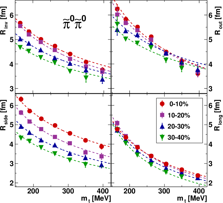
Figure 6: Source radii as function of the transverse mass for pairs of constructed neutral pions as deduced from interpolations of the charged-pion data according to the procedure of Sect. 4.2. The upper left, upper right, lower left, and lower right panels display the ’invariant’, ’out’, ’side’, and ’long’ radii, respectively. Red circles, magenta squares, blue triangles, and green inverted triangles represent the centrality classes $0-10\,\%$, $10-20\,\%$, $20-30\,\%$, and $30-40\,\%$, respectively. Dashed curves are $\chi^{2}$ fits to the data with a function $R=R_{0}(m_{\mathrm{t}}/m_{\pi})^{\alpha}$. The fit parameters $R_{0}$ and $\alpha$ are summarized in table 5.

4.4 Azimuthally-sensitive HBT analysis

To estimate the geometrical quantities hidden in the azimuthal variation of the correlation function (Eq. (7)), we follow the recipe given bei Wiedemann and Heinz Wiedemann_1998 ; Wiedemann_Heinz_1999 and perform a common fit to our data on squared radii from Eq. (10), using the entire set of fit equations (Eqs. (2)) given in ref. e895_2000_phi , which yields the elements of the spatial correlation tensor as ten angle-independent fit parameters:

$$S_{\mu\nu}=\langle\tilde{x}_{\mu}\,\tilde{x}_{\nu}\rangle,\,\,\tilde{x}_{\mu}=x_{\mu}-\langle x_{\mu}\rangle,\hskip 10.03749pt(\mu,\nu=0,\,1,\,2,\,3).$$ (15)

Here, $x_{0}=t$ is the time component, $x_{1}=x$ is parallel to the impact parameter $\bm{b}$, and $x_{3}=z$ points in beam direction. The Cartesian coordinate system is completed with direction $x_{2}=y$ being perpendicular to the reaction plane formed by $x$ and $z$. The brackets $\langle\,\rangle$ indicate an average over the emission source.

A typical fit result is displayed in Fig. 7 for $\pi^{-}\pi^{-}$ pairs with average transverse momentum of $\bar{k}_{\mathrm{t}}=170~{}\mbox{MeV$/c$}$ and for centralities of $10-30\,\%$. It delivers the uncorrected matrix $S$ (in units of fm², with statistical errors attached):

$$S^{\mathrm{\,meas}}=$$

$$\begin{pmatrix}~{}10.12\pm 0.64&-0.77\pm 0.21&-0.15\pm 0.23&~{}~{}~{}0.09\pm 0.14\\ -0.77\pm 0.21&~{}21.60\pm 0.28&-0.07\pm 0.19&~{}~{}~{}2.10\pm 0.11\\ -0.15\pm 0.23&-0.07\pm 0.19&~{}28.87\pm 0.34&-0.05\pm 0.11\\ ~{}~{}~{}0.09\pm 0.14&~{}~{}~{}2.10\pm 0.11&-0.05\pm 0.11&~{}16.12\pm 0.13\end{pmatrix}.$$ (16)

As expected from symmetry considerations Lisa_Heinz_Wiedemann_2000 , only the diagonal elements and $S_{13}$ differ significantly from zero, yielding the following six non-vanishing squared radii

$$R^{2}_{\mathrm{out}}=\, \,\frac{1}{2}(S_{11}+S_{22})+\frac{1}{2}(S_{22}-S_{11})\cos{(2\Phi)}+\langle\beta^{2}_{t}\rangle S_{00},$$

$$R^{2}_{\mathrm{side}}=\, \,\frac{1}{2}(S_{11}+S_{22})+\frac{1}{2}(S_{22}-S_{11})\cos{(2\Phi)},$$

$$R^{2}_{\mathrm{long}}=\, \,S_{33}+\langle\beta^{2}_{l}\rangle S_{00},$$

$$R^{2}_{\mathrm{outside}}=\, \,\frac{1}{2}(S_{22}-S_{11})\sin{(2\Phi)},$$

$$R^{2}_{\mathrm{outlong}}=\, \,S_{13}\cos{(\Phi)},$$

$$R^{2}_{\mathrm{sidelong}}=\, \,-S_{13}\sin{(\Phi)},$$ (17)

where $\beta_{\mathrm{t}}$ and $\beta_{\mathrm{l}}$ are the pair velocities in transverse and longitudinal direction, respectively.

The correction of both, the finite reaction-plane resolution and the finite azimuthal bin width, is performed following the method described in refs. Ollitrault97 ; HBT_in_UrQMD :

$$R^{2,\mathrm{corr}}_{\mathrm{i,n}}=R^{2,\mathrm{meas}}_{\mathrm{i,n}}\,\dfrac{n\,\Delta/2}{F_{\mathrm{n}}\sin(n\,\Delta/2)},$$ (18)

where $R^{2,\mathrm{corr}}_{\mathrm{i,n}}$ ($i=$ ’out’, ’side’, ’long’, ’outside’, ’outlong’, ’sidelong’,  $n=0,\,1,\,2$) are the underlying (“true”) Fourier coefficients HBT_in_UrQMD , $\Delta=\pi/4$ is the present $\Phi$ interval, and the quantity $F_{\mathrm{n}}$ represents the $n$-th event-plane resolution. The values of $F_{1}$ and $F_{2}$ for the centrality classes investigated in the present analysis are summarized in table 1. For the detailed description of the event-plane reconstruction and the centrality dependence of the resolution parameters $F_{\mathrm{n}}$ we refer to a forthcoming HADES paper on the $n$-th ($n\leq 4$) collective flow observables of protons and light nuclei produced in Au + Au collisions at 1.23$A$ GeV hades_flow_AuAu .

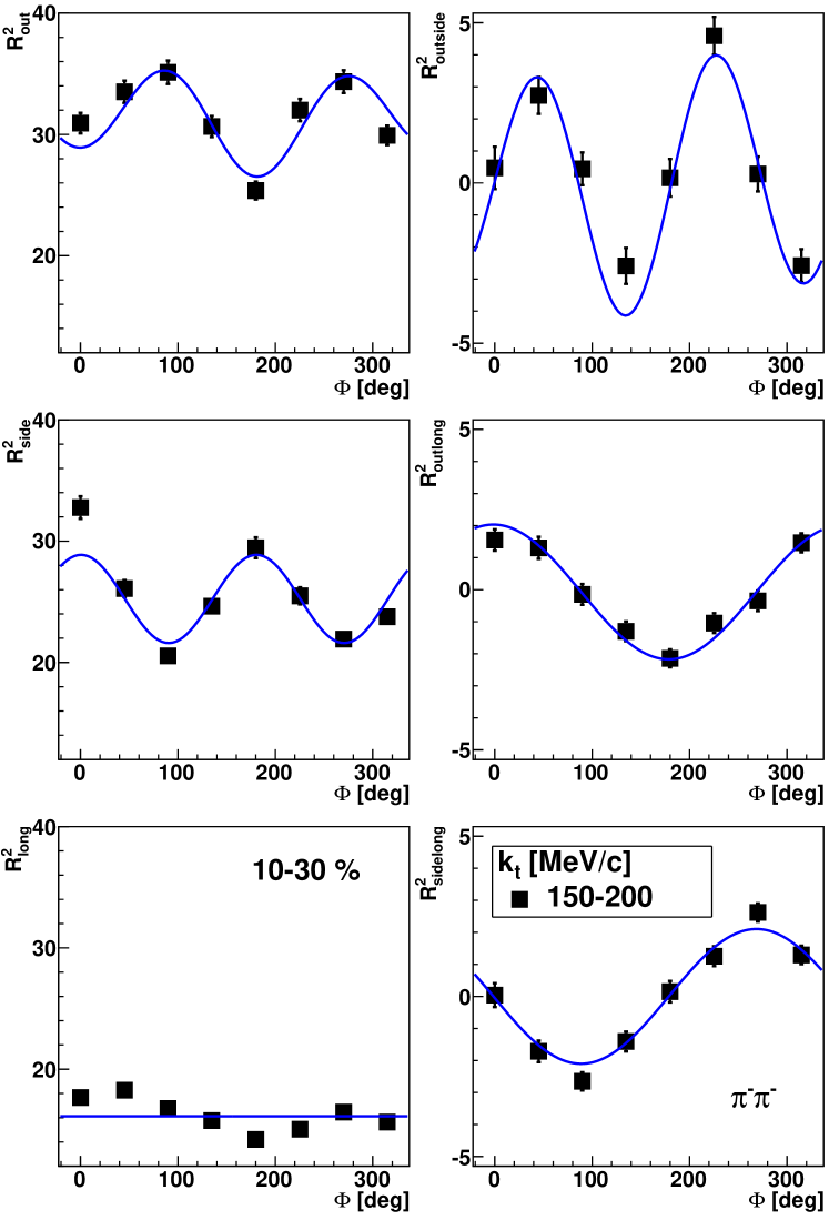
Figure 7: Squared radii as function of the pair azimuthal angle relative to the reaction plane, $\Phi=\phi_{12}-\phi_{\mathrm{RP}}$, for $\pi^{-}\pi^{-}$ pairs with transverse momenta of $p_{\mathrm{t,\,12}}=300-400~{}\mbox{MeV$/c$}$ and for centralities of $10-30\,\%$. The left column from top to bottom shows the ’out’, ’side’, and ’long’ radii. The right column gives the ’outside’, ’outlong’, and ’sidelong’ components. Error bars include only statistical uncertainties. The full curves represent a global fit with Eqs. (2) of ref. e895_2000_phi to the experimental data points.

The matrix $S$ (Eq. (16)) after the correction (Eq. (18)) reads

$$S^{\mathrm{\,corr}}=$$

$$\begin{pmatrix}~{}10.12\pm 0.64&-0.91\pm 0.25&-0.18\pm 0.27&~{}~{}~{}0.09\pm 0.14\\ -0.91\pm 0.25&~{}18.60\pm 0.40&-0.13\pm 0.36&~{}~{}~{}2.49\pm 0.13\\ -0.18\pm 0.27&-0.13\pm 0.36&~{}31.87\pm 0.44&-0.06\pm 0.14\\ ~{}~{}~{}0.09\pm 0.14&~{}~{}~{}2.49\pm 0.13&-0.06\pm 0.14&~{}16.12\pm 0.13\end{pmatrix}.$$ (19)

From this matrix the spatial tilt angle in the reaction plane can be calculated as

$$\theta_{\mathrm{s}}=\frac{1}{2}\tan^{-1}\left(\frac{2S^{\mathrm{\,corr}}_{13}}{S^{\mathrm{\,corr}}_{33}-S^{\mathrm{\,corr}}_{11}}\right)=(-32\pm 2)^{\circ}.$$ (20)

Rotating $S^{\mathrm{\,corr}}$ by the angle $-\theta_{\mathrm{s}}$ around the $y$ axis, i.e. applying the corresponding rotation matrix $G_{y}(\theta_{\mathrm{s}})$, yields a diagonal tensor

$$S^{\mathrm{\,diag}}=G^{{\dagger}}_{y}(\theta_{\mathrm{s}})\cdot S^{\mathrm{\,corr}}\cdot G_{y}(\theta_{\mathrm{s}})=$$

$$\begin{pmatrix}~{}10.12\pm 0.64&-0.73\pm 0.23&-0.18\pm 0.27&~{}~{}~{}0.56\pm 0.18\\ -0.73\pm 0.23&~{}20.15\pm 0.35&-0.15\pm 0.31&~{}~{}~{}0.00\pm 0.23\\ -0.18\pm 0.27&-0.15\pm 0.31&~{}31.87\pm 0.44&~{}~{}~{}0.02\pm 0.22\\ ~{}~{}~{}0.56\pm 0.18&~{}~{}~{}0.00\pm 0.23&~{}~{}~{}0.02\pm 0.22&~{}14.58\pm 0.24\end{pmatrix}$$ (21)

whose eigenvalues are the temporal and geometrical variances $\sigma^{2}_{\mathrm{t}},\sigma^{2}_{\mathrm{x}},\sigma^{2}_{\mathrm{y}},\sigma^{2}_{\mathrm{z}}$. The geometrical variances of $\pi^{-}\pi^{-}$ emission as function of transverse-momentum are displayed in the left column of Fig. 8 for all centralities. Figure 8 also shows the transverse-momentum dependences of the tilt angle, $\theta_{\mathrm{s}}$, the $xy$-eccentricity,

$$\epsilon_{xy}=\frac{\sigma_{\mathrm{y}}^{2}-\sigma_{\mathrm{x}}^{2}}{\sigma_{\mathrm{x}}^{2}+\sigma_{\mathrm{y}}^{2}},$$ (22)

and the $zy$-eccentricity,

$$\epsilon_{zy}=\frac{\sigma_{\mathrm{y}}^{2}-\sigma_{\mathrm{z}}^{2}}{\sigma_{\mathrm{y}}^{2}+\sigma_{\mathrm{z}}^{2}}.$$ (23)

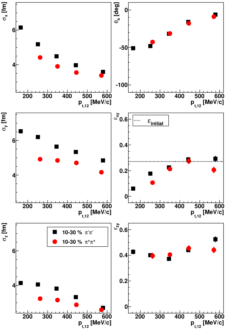
Figure 9: The same as Fig. 8, but for $\pi^{-}\pi^{-}$ (black squares) and $\pi^{+}\pi^{+}$ (red circles) pairs in comparison for medium centralities of $10-30\,\%$.

Note that we included an intermediate centrality class of $25-35\,\%$ to verify the strong centrality dependence of the tilt angle (upper right panel of Fig. 8 and discussion below). For all transverse momenta and all centralities, the deduced eccentricities represent an almond shape in the plane perpendicular to the beam direction. The $xy$-eccentricity becomes smallest (almost circular shape) for most central collisions. Almost no centrality dependence appears for the $zy$-eccentricity. The range of variation with transverse momentum is larger for the $zy$-eccentricity as compared to the one in the $xy$-plane. For large momenta, $\theta_{\mathrm{s}}$ tends to vanish, provided that the 30 % most central event classes (i.e. impact parameters not considerably larger than 50 % of the maximum one) are selected, and the final $\pi^{-}\pi^{-}$ $xy$-eccentricity recovers the corresponding initial eccentricity. No charge-sign difference appears in the transverse-momentum dependence of both, the tilt angle and the eccentricities, while the spatial principal axes differ, as demonstrated in Fig. 9 for medium centralities of $10-30\,\%$.

Due to the freedom in the coordinate-system definition, the tilt angle, defined as the angle between the $z$ coordinate (directed along the shortest principal axis in our case) and the beam direction, can be changed from $\theta_{\mathrm{s}}$ to $\theta_{\mathrm{s}}-90^{o}$, while $\sigma_{x}$ and $\sigma_{z}$ (and accordingly $\epsilon_{xy}$ and $\epsilon_{xy}$) interchange. The arrangement of our data (cf. Fig. 8) was choosen such that both dependences, on transverse momentum and on centrality, show smooth trends. Thus, smaller $|\theta_{\mathrm{s}}|$ for more central collisions are ensured, as one would expect from collision geometry. However, at more peripheral collisions and high values of $p_{\mathrm{t},12}$ a different configuration is conceivably, i.e. requiring $\theta_{\mathrm{s}}=0$ at high transverse momenta (relevant here only for the data points at $p_{\mathrm{t},12}=440\,\mathrm{MeV}/c$ and centrality $25-35\,\%$). Within our statistical and systematic uncertainties we are not able to find a final decision, which arrangement is the better one. (Note also that, near $p_{\mathrm{t},12}=400\,\mathrm{MeV}/c$ and for centralities beyond $20\,\%$, $\sigma_{x}$ and $\sigma_{z}$ are about the same size, which disturbes the picture of a well defined tilt angle, eventually represented by large uncertainties of this quantity.)

The volume of the region of homogeneity,

$$V_{\mathrm{fo}}=(2\pi)^{3/2}\sigma_{\mathrm{x}}\sigma_{\mathrm{y}}\sigma_{\mathrm{z}},$$ (24)

as derived from the spatial principal axes of the Gaussian emission ellipsoid is presented in Fig. 10 (full symbols) as function of transverse momentum for all centrality classes. For comparison, also the results for the approximate volume,

$$V_{\mathrm{fo}}^{\prime}=(2\pi)^{3/2}R^{2}_{\mathrm{side}}R_{\mathrm{long}},$$ (25)

following from the azimuthally-integrated analysis (open symbols) is shown. Differences are significant only at small transverse momenta, where the tilt angle vanishes.

To study the centrality dependence of the tilt angle in more detail, Fig. 11 displays $\theta_{\mathrm{s}}$ for $\pi^{-}\pi^{-}$ (full symbols) and $\pi^{+}\pi^{+}$ (open symbols) pairs as function of the impact parameter, $b$ (cf. table 1), for different average transverse momentum values. While for lower momenta the magnitude of $\theta_{\mathrm{s}}$ is proportional to $b$, this dependence gets weaker with increasing pair transverse momentum until the tilt is close to zero for the highest momentum classes. No charge-sign difference is observed in the centrality dependence of $\theta_{\mathrm{s}}$.

Figure 12 explicitly relates the $xy$-eccentricity for $\pi^{-}\pi^{-}$ pairs to the initial eccentricity relative to the participant plane (cf. Eq. (21) of ref. STAR2015 ), as derived from Glauber simulations PhobosGlauber2015 . For large transverse momenta the source eccentricity derived from the present identical-pion HBT analysis recovers the inital (nucleon) eccentricity. This observation is essentially different from the picture at higher energies, where the $k_{\mathrm{t}}$ integrated freeze-out eccentricity is found considerably below the corresponding initial one STAR2015 ; PHENIX2014 ; ALICE2017 . The trend of increasing freeze-out eccentricity with increasing transverse momentum is also found by ALICE at LHC, though on a much lower absolute scale ALICE2017 . The model of (3+1)D hydrodynamics Kisiel2014 slightly unterestimates the final source eccentricity at LHC. It would be very desirable to discuss in separate future works the present observations at SIS18 energies in the framework of contemporary hydro or transport models.

Fig. 13 shows the temporal components of the spatial correlation tensor (cf. Eqs. (2) of ref. e895_2000_phi ). For the emission duration, $\sigma_{\mathrm{t}}^{2}=S_{00}$, the fit yields values significantly deviating from zero, especially for low transverse momenta and for all considered centrality classes except the most central one. The values for the mixed elements, however, are much smaller and are mostly consistent with zero, with the possible exception of pion pairs with small transverse momenta in central collisions. As already mentioned above, the disappearance of $S_{01}$, $S_{02}$ and $S_{03}$ is expected due to symmetry reasons Lisa_Heinz_Wiedemann_2000 . However, one should keep in mind that the symmetry of the rapidity distribution w.r.t. midrapidity is not perfect in the present fixed-target experiment, even though the rapidity interval was rather restricted for this analysis ($|y-y_{cm}|<0.35$).

Finally, the geometrical and temporal variances and the tilt angle of the $\pi^{-}\pi^{-}$ ($\pi^{+}\pi^{+}$) emission source in dependence of centrality and transverse momentum are summarized in table 6 (7).

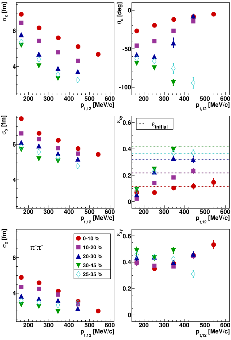
Figure 8: The spatial principal axes (left column),the tilt angle w.r.t. the beam axis in the reaction plane (Eq. (20), top right), the $xy$-eccentricity (Eq. (22, center right), and the $zy$-eccentricity (Eq. (23, bottom right) of the Gaussian emission ellipsoid of $\pi^{-}\pi^{-}$ pairs as function of pair transverse momentum for different centrality classes (cf. legend). Error bars include only statistical uncertainties. Dotted lines represent the corresponding initial eccentricity as derived from Glauber simulations.

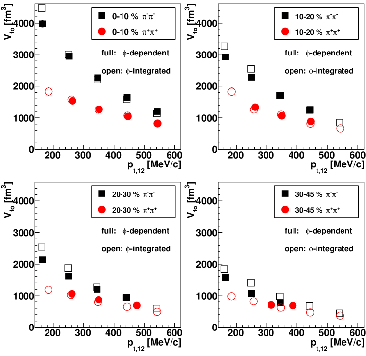
Figure 10: The volume of the region of homogeneity (Eq. (24), full symbols) as derived from the azimuthally-sensitive analysis and the approximate volume (Eq. (25), open symbols) following from the azimuthally-integrated analysis of $\pi^{-}\pi^{-}$ (squares) and $\pi^{+}\pi^{+}$ (circles) pairs as function of pair transverse momentum for different centralities (cf. legend).

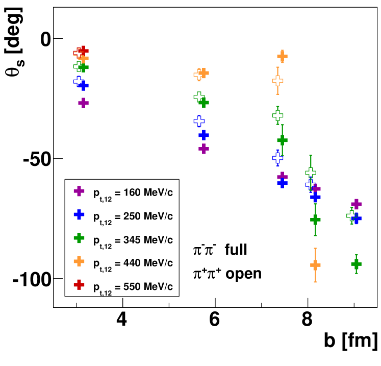
Figure 11: The emission-ellipsoid tilt angle, $\theta_{\mathrm{s}}$, in the reaction plane for $\pi^{-}\pi^{-}$ (full symbols) and $\pi^{+}\pi^{+}$ (open symbols) pairs as function of the mean impact parameter derived from Glauber MC calculations hades_centrality:2018am for different pair transverse momentum classes. Error bars include only statistical uncertainties.

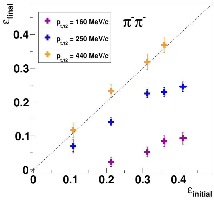
Figure 12: The $\pi^{-}\pi^{-}$ emission ellipsoid $xy$-eccentricity (Eq. (22)) as function of the initial nucleon eccentricity derived from Glauber simulations PhobosGlauber2015 for different pair transverse momentum classes. Error bars include only statistical uncertainties. The dashed line indicates $\epsilon_{\mathrm{final}}=\epsilon_{\mathrm{initial}}$.

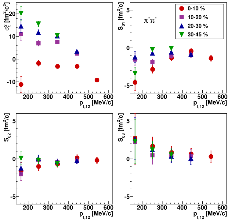
Figure 13: The temporal components of the spatial correlation tensor $S$ (Eq. (15)) for $\pi^{-}\pi^{-}$ pairs as function of transverse momentum for different centrality classes (cf. legend). The upper left, upper right, lower left, and lower right panels display $\sigma_{\mathrm{t}}^{2}=S_{00}$, $S_{01}$, $S_{02}$, and $S_{03}$, respectively. Error bars include only statistical uncertainties.

4.5 Comparison with other experiments - Excitation functions of source parameters

The energy dependences below $\sqrt{s_{\mathrm{NN}}}=4$ GeV of the $\pi^{-}\pi^{-}$ emission ellipsoid principal axes, the tilt angle w.r.t. the beam axis in the reaction plane, the eccentricities, and the emission duration for medium centralities and average transverse momentum of $\bar{k}_{\mathrm{t}}=110~{}\mbox{MeV$/c$}$ are shown in Fig. 14. The displayed HADES/SIS18 data follow the trends of the E895/AGS data e895_2000_phi .

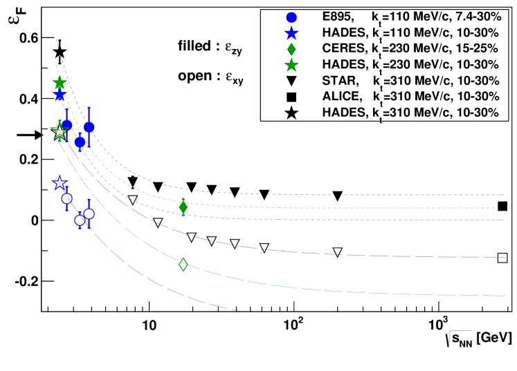
Figure 15: Excitation function of the final $\pi^{-}\pi^{-}$ eccentricities $\epsilon_{xy}$ (open symbols) and $\epsilon_{zy}$ (filled symbols) for mid-central ($10-30\,\%$) Au + Au, Pb + Au, or Pb + Pb collisions. Stars are HADES data for three different transverse momentum intervals with average values of $\bar{k}_{\mathrm{t}}=110$, 230, and 310 MeV$/c$. The circles, diamond, triangles, and square are corresponding data by E895 at AGS e895_2000_phi , CERES at SPS CERES2008 , STAR at RHIC STAR2015 , and ALICE at LHC ALICE2017 , respectively. Error bars include only statistical uncertainties. Short (long) dashed curves connecting the filled (open) symbols are to guide the eyes. The arrow (to be compared to the open symbols) indicates the initial eccentricity derived from Glauber simulations PhobosGlauber2015 .

The excitation function of eccentricities over a wider range of collision energies is presented in Fig. 15. While for the HADES and E895 data the exact equations (22) and (23) are applied (cp. Fig. 14), for $\sqrt{s_{\mathrm{NN}}}>4$ GeV, where no $\pi\pi$ emission source data after principal-axis transformation of the spatial correlation tensor are available, the approximations $\epsilon_{\mathrm{xy}}\approx 2R^{2}_{\mathrm{side,\,2}}/R^{2}_{\mathrm{side,\,0}}$ and $\epsilon_{zy}\approx 1-2R^{2}_{\mathrm{long,\,0}}/(R^{2}_{\mathrm{side,\,0}}+2R^{2}_{\mathrm{side,\,2}}+R^{2}_{\mathrm{long,\,0}})$ are used. Here, the quantities $R^{2}_{\mathrm{side,\,0}}$ ($R^{2}_{\mathrm{long,\,0}}$) and $R^{2}_{\mathrm{side,\,2}}$ are the zeroth- and 2nd-order Fourier coefficients of the azimuthal-angle parameterization of the ’side’ (’long’) radius, respectively, where $2R^{2}_{\mathrm{side,\,2}}$ corresponds to the oscillation amplitude of both the squared ’out’ and ’side’ radii (cf. Eqs. (17) and Fig. 7). These approximations are justified by the small tilt angles found at high collision energies. We observe a remarkable increase of both types of eccentricity at low $\sqrt{s_{\mathrm{NN}}}$. It would be very desirable to study the strong increase towards low energy of both eccentricity and tilt angle in the framework of contemporary models. First investigations of both observables by means of several theoretical transport calculations qualitatively reproduced the experimental findings Lisa2011 ; the quantitative reproduction of their dependences on collision energy, centrality and transverse momentum should allow for further discrimination among the models.

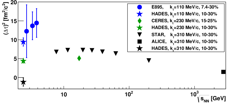
Figure 16: Excitation function of the squared emission duration, the latter one either directly taken from the corresponding fit parameter of the spatial correlation tensor, $\sigma_{\mathrm{t}}^{2}=S_{00}$ (cf. Eqs. (17)), or derived from the difference of the ’out’ and ’side’ radii, $(\Delta\tau)^{2}=(R^{2}_{\mathrm{out}}-R^{2}_{\mathrm{side}})/\langle\beta_{t}^{2}\rangle$, for mid-central ($10-30\,\%$) Au + Au collisions. Stars are HADES $\pi^{-}\pi^{-}$ data of $\sigma_{\mathrm{t}}^{2}$ for three different transverse momentum regions with average values of $\bar{k}_{\mathrm{t}}=110$, 230, and 310 MeV$/c$. The circles are corresponding $\sigma_{\mathrm{t}}^{2}$ data by E895 at AGS e895_2000_phi . The diamond, triangles, and square represent data of $(\Delta\tau)^{2}$ by CERES at SPS CERES2008 , STAR at RHIC STAR2015 , and ALICE at LHC ALICE2017 , respectively. Error bars include only statistical uncertainties.

The excitation function of the squared emission duration which is either taken directly from the fit parameter $S_{00}$, i.e. the temporal variance of the $\pi\pi$ emission (cf. Eqs. (17)), or from the difference of the squared ’out’ and ’side’ radii, $(\Delta\tau)^{2}=(R_{\mathrm{out}}^{2}-R_{\mathrm{side}}^{2})/\langle\beta^{2}_{\mathrm{t}}\rangle$, is shown in Fig. 16. For all data of the various experiments, the emission duration appears small, i.e. typically a few fm/$c$. With increasing transverse momentum, the emission duration deduced from the HADES data is found to decrease, virtually vanishing for large momenta. Taking the data points at $k_{\mathrm{t}}=310~{}\mbox{MeV$/c$}$, there is a clear energy dependence: A rise towards $\sqrt{s_{\mathrm{NN}}}\sim 10-20$ GeV and then a a slow drop towards LHC.

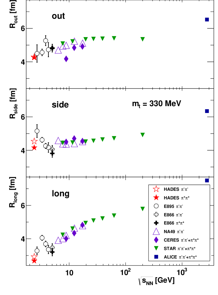
Figure 17: Excitation function of the source radii $R_{\mathrm{out}}$ (upper panel), $R_{\mathrm{side}}$ (central panel), and $R_{\mathrm{long}}$ (lower panel) for the azimuthally-integrated correlation function of pairs of identical pions with transverse mass of $m_{t}=330~{}\mbox{MeV}$ in central ($0-10\,\%$) collisions of Au + Au or Pb + Pb. Squares represent data by ALICE at LHC ($\pi^{+}\pi^{+}$) ALICE2011 , full triangles STAR at RHIC ($\pi^{-}\pi^{-}$+$\pi^{+}\pi^{+}$) STAR2015 , diamonds are for CERES at SPS ($\pi^{-}\pi^{-}$+$\pi^{+}\pi^{+}$) CERES_2003 , open triangles are for NA49 at SPS ($\pi^{-}\pi^{-}$) NA49_2008 , open circles are $\pi^{-}\pi^{-}$ data by E895 at AGS e895_2000 ; pipi_imaging_E895 , and open (full) crosses involve $\pi^{-}\pi^{-}$ ($\pi^{+}\pi^{+}$) data of E866 at AGS e866_1999 , respectively. The present data of HADES at SIS18 for pairs of $\pi^{-}\pi^{-}$ ($\pi^{+}\pi^{+}$) are given as open (full) stars. Statistical errors are displayed as error bars; if not visible, they are smaller than the corresponding symbols. Note the suppressed zero on the ordinate.

Finally, we return to a few results of the azimuthally-integrated HBT analysis, concentrating on central collisions ($0-10\,\%$). The excitation functions of $R_{\mathrm{out}}$, $R_{\mathrm{side}}$, and $R_{\mathrm{long}}$ for pion pairs produced in most central events are displayed in Fig. 17. All shown radius parameters have been obtained by interpolating the existing measured data points to the same transverse mass of $m_{\mathrm{t}}=330~{}\mbox{MeV}$ ($k_{\mathrm{t}}=300~{}\mbox{MeV$/c$}$) at which the charge differences of the source radii almost vanish (cf. Fig. 4). The statistical errors are properly propagated and quadratically added to the differences between linear and cubic-spline interpolations. Extrapolations were not necessary at this $m_{\mathrm{t}}$ value. $R_{\mathrm{out}}$ and $R_{\mathrm{side}}$ vary not more than 40 % over three orders of magnitude in center-of-mass energy. Only $R_{\mathrm{long}}$ exhibits a steady increase by about a factor of two when going in energy from SIS18 via AGS, SPS, RHIC to LHC. Note that in the excitation functions shown in ref. STAR2015 not all, particularly AGS, data points were properly corrected for their $k_{\mathrm{t}}$ dependence.

The excitation function of $R_{\mathrm{out}}^{2}-R_{\mathrm{side}}^{2}$ for an average transverse momentum of the pion pairs of $k_{\mathrm{t}}=300~{}\mbox{MeV$/c$}$ in central collisions is shown in Fig. 18. Almost all other measurements below 10 GeV are characterized by large errors and scatter sizeably. The new HADES data show that the difference of the source parameters in the transverse plane almost vanishes at low collision energies. Since this quantity is related to the emission duration via Eqs. (17), one would conclude that in the 1$A$ GeV energy region the observed pions are emitted into free space during a short time span of less than a few fm/$c$ (cp. also Figs. 14 (bottom right) and 16 displaying similar data divided by $\langle\beta^{2}_{\mathrm{t}}\rangle$ for centralities of $0-10\,\%$ and $10-30\,\%$, respectively, but for different transverse momenta). However, also the opaqueness of the source affects $R_{\mathrm{out}}^{2}-R_{\mathrm{side}}^{2}$ which could cause it to become negative, thus compensating the positive contribution of the emission duration Barz99 . We also emphasize that, with increasing available energy, this quantity reaches a local maximum at $\sqrt{s_{\mathrm{NN}}}\sim 20-30$ GeV and afterwards decreases towards zero at LHC energies.

The excitation function of the approximate volume of the region of homogeneity, Eq. (25), for central collisions is given in Fig. 19. Here, we chose this approximation, in contrast to Eq. (24), for the sake of comparability with other experiments. Note that this definition of a three-dimensional Gaussian volume does not incorporate $R_{\mbox{{\scriptsize out}}}$ since this length is potentially extended due to a finite value of the aforementioned emission duration. For the large transverse momenta selected, the differences of the azimuthally-integrated and azimuthally-sensitive analyses as well as the charge-sign splitting largely vanish, cp. Fig. 10 exhibiting the strong transverse-momentum dependence of the volume, especially for $\pi^{-}\pi^{-}$ pairs. From the above HADES data, we estimate a volume of about 850 fm³ for constructed $\tilde{\pi}^{0}\tilde{\pi}^{0}$ pairs. This volume of homogeneity steadily increases with energy, but appears merely a factor four larger at LHC. Extrapolating the volume to $k_{\mathrm{t}}=0$ yields a value of about 3,900 fm³.

Similar excitation functions at other transverse momenta or centralities (with proper interpolation/extrapolation of the transverse-momentum and centrality dependences) can be derived from the source parameters summarized in tables 2, 3, 6, and 7.

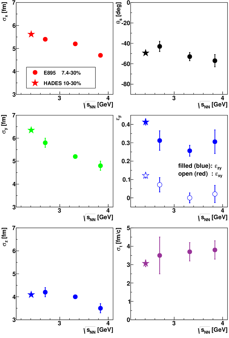
Figure 14: The low-energy excitation function of the principal axes (left column), the tilt angle in the reaction plane (Eq. (20), top right), the eccentricities $\epsilon_{xy}$ (Eq. (22), center right, open symbols) and $\epsilon_{zy}$ (Eq. (23), center right, filled symbols), and the emission duration $\sigma_{\mathrm{t}}=\sqrt{S_{00}}$ (Eqs. (17), bottom right) as derived from the Gaussian emission ellipsoid of $\pi^{-}\pi^{-}$ pairs. Stars are HADES data for centralities of $10-30\,\%$ and average transverse momentum of $\bar{k}_{\mathrm{t}}=110~{}\mbox{MeV$/c$}$. The circles are corresponding E895 data for slightly different centralities taken at beam energies of 2, 4, and 6 $A$ GeV e895_2000_phi . Error bars include only statistical uncertainties.

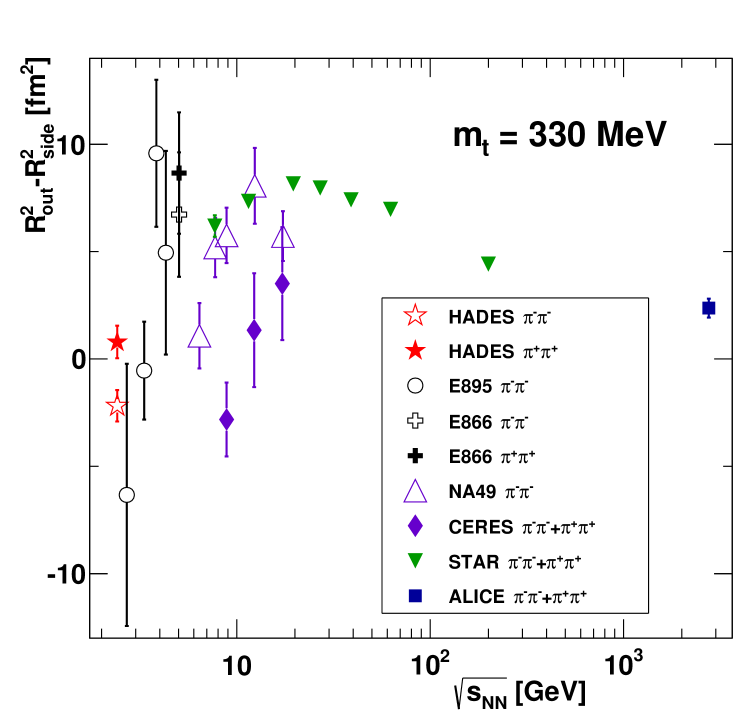
Figure 18: The same as Fig. 17, but for the derived quantity $R_{\mathrm{out}}^{2}-R_{\mathrm{side}}^{2}$.

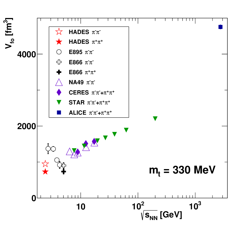
Figure 19: The same as Fig. 17, but for the derived approximate volume of the region of homogeneity, Eq. (25).

5 Summary and outlook

We presented high-statistics $\pi^{-}\pi^{-}$ and $\pi^{+}\pi^{+}$ HBT data for Au + Au collisions at 1.23$A$ GeV. The three-dimensional Gaussian emission source is studied in dependence on transverse momentum and collision centrality. It is found to follow the trends observed at higher collision energies, extending the corresponding excitation functions towards very low energies. A surprisingly small variation of the space-time extent of the pion emission source over three orders of magnitude of $\sqrt{s_{\mathrm{NN}}}$ is observed. All source radii increase almost linearly with the number of participants, irrespective of transverse momentum. Substantial differences of the source radii for pairs of negatively and positively charged pions, especially at low transverse momenta, are found, an effect hardly visible at higher collision energies. Correcting for this Coulomb effect, we found for all transverse momenta and centralities a stable hierarchy of the three widths of the emission ellipsoid, revealing an oblate shape in coordinate space with the largest extent oriented perpendicular to the reaction-plane. The corresponding eccentricity is found to recover the initial geometrical eccentricity of the nucleons if sufficiently large transverse momenta of the pions are considered. For low momenta, the shape approaches a circular one. Selecting collisions of the 30 % most central event classes, the tilt angle in the reaction plane, $\theta_{\mathrm{s}}$, is found to approach zero at high $p_{\mathrm{t}}$. For low transverse momenta, $|\theta_{\mathrm{s}}|$ increases and its $p_{\mathrm{t}}$ dependence is stronger for larger impact parameters. The centrality dependences of the tilt angle and of the eccentricity are found to be independent of pion charge and transverse momentum. Both quantities fit well into a corresponding low-energy excitation function for semi-central collisions e895_2000_phi .

Future femtoscopic studies of other system-energy combinations in the ’low-energy domain’, e.g. performed with HADES + CBM at FAIR/GSI CBM2017 and MPD at NICA in Dubna NICA or with the STAR fixed-target program KMeehan_STAR_2017 , may focus also on correlations of other particles (pp, p$\Lambda$, $\Lambda\Lambda$, etc.), allowing for deeper insight into their strong interaction CATS2018 .

Table 2: Source parameters resulting from fits with Eqs. (5) and (7) for $\pi^{-}\pi^{-}$ pairs in dependence of centrality and average transverse momentum, $\bar{k}_{\mathrm{t}}$. Values in the 1st (2nd) brackets represent the corresponding statistical (systematic) uncertainties in units of the last digit of the respective quantity.

Centrality	$\bar{k}_{\mathrm{t}}$	$R_{\mathrm{inv}}$	$\lambda_{\mathrm{inv}}$	$R_{\mathrm{out}}$	$R_{\mathrm{side}}$	$R_{\mathrm{long}}$	$\lambda_{\mathrm{osl}}$
(%)	(MeV$/c$)	(fm)		(fm)	(fm)	(fm)
0-10	43	$7.03(23)(^{+17}_{-10})$	$0.904(84)(^{+42}_{-38})$	$7.03(60)(^{+31}_{-8})$	$7.44(27)(^{+23}_{-0})$	$5.50(34)(^{+21}_{-2})$	$0.872(74)(^{+59}_{-0})$
0-10	81	$6.54(4)(^{+20}_{-0})$	$0.801(12)(^{+30}_{-0})$	$6.88(9)(^{+17}_{-1})$	$7.15(10)(^{+16}_{-1})$	$5.53(5)(^{+11}_{-1})$	$0.904(19)(^{+18}_{-2})$
0-10	125	$5.88(2)(^{+28}_{-4})$	$0.710(7)(^{+59}_{-6})$	$6.22(5)(^{+23}_{-1})$	$6.27(6)(^{+21}_{-1})$	$4.81(3)(^{+15}_{-0})$	$0.848(11)(^{+36}_{-1})$
0-10	172	$5.37(2)(^{+28}_{-14})$	$0.662(7)(^{+65}_{-21})$	$5.59(6)(^{+26}_{-8})$	$5.75(5)(^{+15}_{-7})$	$4.17(2)(^{+15}_{-5})$	$0.840(12)(^{+40}_{-13})$
0-10	221	$5.01(3)(^{+26}_{-17})$	$0.628(9)(^{+72}_{-26})$	$5.16(10)(^{+18}_{-9})$	$5.26(6)(^{+13}_{-8})$	$3.61(3)(^{+12}_{-5})$	$0.847(19)(^{+39}_{-17})$
0-10	271	$4.57(4)(^{+22}_{-17})$	$0.565(12)(^{+74}_{-24})$	$4.69(34)(^{+16}_{-13})$	$4.80(8)(^{+11}_{-10})$	$3.11(3)(^{+11}_{-6})$	$0.836(62)(^{+43}_{-24})$
0-10	321	$4.25(6)(^{+15}_{-15})$	$0.530(18)(^{+67}_{-20})$	$4.27(11)(^{+12}_{-8})$	$4.32(9)(^{+8}_{-6})$	$2.80(5)(^{+8}_{-11})$	$0.846(26)(^{+15}_{-15})$
0-10	370	$3.91(10)(^{+35}_{-14})$	$0.462(27)(^{+110}_{-19})$	$3.84(27)(^{+20}_{-12})$	$3.95(13)(^{+14}_{-8})$	$2.50(7)(^{+15}_{-5})$	$0.776(57)(^{+57}_{-20})$
0-10	420	$3.84(15)(^{+28}_{-11})$	$0.494(44)(^{+73}_{-15})$	$3.04(19)(^{+25}_{-4})$	$3.57(19)(^{+25}_{-12})$	$2.33(9)(^{+18}_{-0})$	$0.725(52)(^{+68}_{-3})$
10-20	43	$6.08(23)(^{+28}_{-15})$	$0.734(75)(^{+82}_{-31})$	$4.82(73)(^{+69}_{-26})$	$6.24(24)(^{+14}_{-12})$	$5.73(39)(^{+37}_{-13})$	$0.740(72)(^{+30}_{-30})$
10-20	81	$6.16(4)(^{+9}_{-1})$	$0.770(13)(^{+28}_{-1})$	$6.29(8)(^{+8}_{-0})$	$6.09(8)(^{+5}_{-0})$	$5.57(6)(^{+8}_{-0})$	$0.849(18)(^{+17}_{-0})$
10-20	125	$5.71(3)(^{+22}_{-2})$	$0.702(9)(^{+50}_{-3})$	$5.94(5)(^{+17}_{-1})$	$5.73(5)(^{+11}_{-0})$	$4.89(3)(^{+11}_{-0})$	$0.829(12)(^{+26}_{-1})$
10-20	172	$5.21(3)(^{+22}_{-7})$	$0.666(9)(^{+61}_{-10})$	$5.57(6)(^{+17}_{-2})$	$5.09(5)(^{+12}_{-2})$	$4.14(3)(^{+12}_{-1})$	$0.845(13)(^{+34}_{-3})$
10-20	221	$4.78(4)(^{+24}_{-13})$	$0.629(12)(^{+73}_{-19})$	$5.06(10)(^{+17}_{-7})$	$4.66(6)(^{+7}_{-6})$	$3.60(3)(^{+8}_{-4})$	$0.868(20)(^{+31}_{-14})$
10-20	270	$4.32(5)(^{+25}_{-11})$	$0.585(16)(^{+88}_{-17})$	$4.62(33)(^{+15}_{-11})$	$4.19(8)(^{+10}_{-7})$	$3.03(4)(^{+6}_{-4})$	$0.885(65)(^{+49}_{-19})$
10-20	320	$4.03(8)(^{+29}_{-10})$	$0.529(25)(^{+100}_{-15})$	$4.11(13)(^{+23}_{-9})$	$3.62(10)(^{+30}_{-6})$	$2.73(6)(^{+11}_{-4})$	$0.827(31)(^{+81}_{-18})$
10-20	370	$3.52(14)(^{+60}_{-4})$	$0.435(35)(^{+118}_{-5})$	$3.37(23)(^{+44}_{-15})$	$3.27(15)(^{+11}_{-4})$	$2.43(8)(^{+38}_{-2})$	$0.736(53)(^{+133}_{-10})$
20-30	43	$5.62(22)(^{+27}_{-13})$	$0.821(86)(^{+56}_{-40})$	$4.22(74)(^{+118}_{-4})$	$5.49(22)(^{+27}_{-2})$	$5.76(44)(^{+55}_{-2})$	$0.790(80)(^{+108}_{-4})$
20-30	81	$5.69(4)(^{+16}_{-0})$	$0.745(14)(^{+34}_{-0})$	$5.76(8)(^{+16}_{-0})$	$5.46(7)(^{+9}_{-0})$	$5.39(6)(^{+17}_{-0})$	$0.823(18)(^{+22}_{-0})$
20-30	124	$5.28(3)(^{+24}_{-2})$	$0.701(10)(^{+48}_{-2})$	$5.56(5)(^{+20}_{-0})$	$5.06(5)(^{+13}_{-0})$	$4.62(4)(^{+16}_{-0})$	$0.822(12)(^{+29}_{-0})$
20-30	172	$4.87(3)(^{+22}_{-9})$	$0.670(10)(^{+62}_{-13})$	$5.37(6)(^{+16}_{-3})$	$4.53(5)(^{+13}_{-2})$	$3.89(3)(^{+12}_{-2})$	$0.851(14)(^{+34}_{-4})$
20-30	221	$4.45(4)(^{+24}_{-13})$	$0.622(14)(^{+81}_{-19})$	$4.84(10)(^{+10}_{-6})$	$4.21(6)(^{+9}_{-4})$	$3.32(4)(^{+5}_{-3})$	$0.861(21)(^{+16}_{-10})$
20-30	270	$4.03(7)(^{+34}_{-17})$	$0.543(20)(^{+104}_{-24})$	$4.68(35)(^{+22}_{-9})$	$3.65(8)(^{+16}_{-5})$	$2.80(5)(^{+10}_{-3})$	$0.867(66)(^{+65}_{-16})$
20-30	320	$3.98(10)(^{+21}_{-9})$	$0.565(34)(^{+72}_{-14})$	$4.13(16)(^{+25}_{-18})$	$3.42(12)(^{+15}_{-9})$	$2.58(7)(^{+4}_{-5})$	$0.868(40)(^{+60}_{-23})$
20-30	370	$3.57(18)(^{+73}_{-9})$	$0.480(50)(^{+180}_{-12})$	$3.74(31)(^{+38}_{-18})$	$3.03(15)(^{+7}_{-0})$	$2.41(10)(^{+3}_{-8})$	$0.932(82)(^{+9}_{-6})$
30-40	43	$5.02(23)(^{+26}_{-9})$	$0.711(89)(^{+42}_{-14})$	$3.74(45)(^{+17}_{-12})$	$5.18(23)(^{+12}_{-0})$	$4.96(58)(^{+44}_{-9})$	$0.721(86)(^{+42}_{-10})$
30-40	81	$5.10(5)(^{+26}_{-0})$	$0.707(16)(^{+36}_{-0})$	$5.22(8)(^{+18}_{-2})$	$4.85(7)(^{+12}_{-2})$	$4.98(7)(^{+24}_{-2})$	$0.784(19)(^{+20}_{-3})$
30-40	125	$4.89(3)(^{+24}_{-1})$	$0.691(12)(^{+41}_{-1})$	$5.26(6)(^{+19}_{-0})$	$4.53(5)(^{+9}_{-0})$	$4.34(4)(^{+15}_{-0})$	$0.811(14)(^{+20}_{-0})$
30-40	172	$4.52(4)(^{+27}_{-6})$	$0.664(13)(^{+73}_{-10})$	$5.10(7)(^{+19}_{-3})$	$4.11(5)(^{+19}_{-2})$	$3.64(4)(^{+17}_{-2})$	$0.849(16)(^{+44}_{-4})$
30-40	221	$4.20(5)(^{+24}_{-12})$	$0.648(17)(^{+81}_{-18})$	$4.64(10)(^{+13}_{-3})$	$3.72(6)(^{+16}_{-2})$	$3.07(4)(^{+6}_{-2})$	$0.872(23)(^{+17}_{-6})$
30-40	270	$3.81(8)(^{+37}_{-18})$	$0.562(25)(^{+129}_{-26})$	$4.24(28)(^{+41}_{-7})$	$3.24(9)(^{+15}_{-4})$	$2.66(6)(^{+11}_{-2})$	$0.851(58)(^{+75}_{-11})$
30-40	320	$3.38(13)(^{+61}_{-8})$	$0.480(36)(^{+155}_{-11})$	$4.03(19)(^{+30}_{-18})$	$2.86(12)(^{+38}_{-8})$	$2.37(8)(^{+11}_{-12})$	$0.855(47)(^{+39}_{-23})$

Table 3: The same as table 2, but for $\pi^{+}\pi^{+}$ pairs.

Centrality	$\bar{k}_{\mathrm{t}}$	$R_{\mathrm{inv}}$	$\lambda_{\mathrm{inv}}$	$R_{\mathrm{out}}$	$R_{\mathrm{side}}$	$R_{\mathrm{long}}$	$\lambda_{\mathrm{osl}}$
(%)	(MeV$/c$)	(fm)		(fm)	(fm)	(fm)
0-10	92	$4.81(16)(^{+39}_{-0})$	$0.870(65)(^{+80}_{-0})$	$5.67(40)(^{+51}_{-3})$	$5.45(24)(^{+22}_{-4})$	$4.04(17)(^{+26}_{-2})$	$0.973(71)(^{+23}_{-5})$
0-10	130	$4.70(4)(^{+39}_{-5})$	$0.697(14)(^{+81}_{-7})$	$5.32(7)(^{+40}_{-1})$	$5.05(7)(^{+20}_{-1})$	$3.87(4)(^{+22}_{-1})$	$0.876(17)(^{+40}_{-1})$
0-10	175	$4.54(3)(^{+31}_{-14})$	$0.614(10)(^{+89}_{-20})$	$5.23(7)(^{+36}_{-8})$	$4.79(6)(^{+16}_{-7})$	$3.39(3)(^{+20}_{-4})$	$0.830(14)(^{+60}_{-12})$
0-10	223	$4.37(4)(^{+36}_{-17})$	$0.556(11)(^{+104}_{-23})$	$4.86(9)(^{+26}_{-11})$	$4.62(6)(^{+14}_{-9})$	$3.13(3)(^{+13}_{-6})$	$0.815(19)(^{+43}_{-17})$
0-10	272	$4.17(5)(^{+34}_{-19})$	$0.525(15)(^{+101}_{-25})$	$4.44(9)(^{+40}_{-9})$	$4.28(8)(^{+15}_{-7})$	$2.82(4)(^{+14}_{-4})$	$0.809(22)(^{+65}_{-15})$
0-10	321	$3.86(7)(^{+37}_{-17})$	$0.489(19)(^{+111}_{-23})$	$4.16(12)(^{+30}_{-17})$	$4.06(9)(^{+10}_{-9})$	$2.55(5)(^{+8}_{-5})$	$0.835(28)(^{+66}_{-21})$
0-10	371	$3.57(10)(^{+35}_{-12})$	$0.440(26)(^{+71}_{-14})$	$3.71(17)(^{+65}_{-27})$	$3.78(12)(^{+22}_{-7})$	$2.23(6)(^{+11}_{-6})$	$0.817(37)(^{+114}_{-25})$
0-10	421	$3.46(17)(^{+26}_{-9})$	$0.376(37)(^{+54}_{-9})$	$3.28(22)(^{+48}_{-24})$	$3.55(19)(^{+10}_{-12})$	$2.12(9)(^{+4}_{-14})$	$0.723(48)(^{+17}_{-0})$
10-20	92	$4.86(18)(^{+9}_{-3})$	$0.851(70)(^{+25}_{-6})$	$5.47(46)(^{+11}_{-6})$	$5.07(21)(^{+2}_{-15})$	$4.48(24)(^{+15}_{-5})$	$0.963(83)(^{+28}_{-10})$
10-20	129	$4.63(5)(^{+33}_{-5})$	$0.678(16)(^{+77}_{-6})$	$5.32(8)(^{+24}_{-2})$	$4.52(7)(^{+11}_{-1})$	$3.88(5)(^{+22}_{-1})$	$0.836(19)(^{+42}_{-2})$
10-20	174	$4.53(4)(^{+26}_{-10})$	$0.635(13)(^{+71}_{-14})$	$5.08(7)(^{+24}_{-5})$	$4.42(6)(^{+14}_{-4})$	$3.54(4)(^{+15}_{-3})$	$0.833(16)(^{+50}_{-6})$
10-20	222	$4.31(5)(^{+27}_{-15})$	$0.587(15)(^{+84}_{-20})$	$4.78(10)(^{+21}_{-6})$	$4.04(6)(^{+16}_{-4})$	$3.14(4)(^{+10}_{-3})$	$0.828(21)(^{+43}_{-9})$
10-20	271	$4.05(6)(^{+22}_{-15})$	$0.549(19)(^{+76}_{-20})$	$4.38(11)(^{+28}_{-8})$	$3.87(8)(^{+11}_{-6})$	$2.80(5)(^{+10}_{-4})$	$0.837(26)(^{+42}_{-15})$
10-20	321	$3.71(10)(^{+43}_{-8})$	$0.477(27)(^{+111}_{-11})$	$4.05(14)(^{+4}_{-16})$	$3.49(11)(^{+9}_{-4})$	$2.40(6)(^{+3}_{-2})$	$0.796(33)(^{+25}_{-10})$
10-20	371	$3.80(16)(^{+25}_{-28})$	$0.474(44)(^{+41}_{-35})$	$4.51(33)(^{+34}_{-73})$	$3.38(16)(^{+0}_{-14})$	$2.35(9)(^{+16}_{-6})$	$0.951(63)(^{+121}_{-34})$
20-30	92	$4.29(19)(^{+45}_{-1})$	$0.721(67)(^{+91}_{-1})$	$4.71(54)(^{+23}_{-1})$	$4.34(21)(^{+15}_{-1})$	$4.01(25)(^{+19}_{-1})$	$0.774(76)(^{+34}_{-0})$
20-30	129	$4.36(6)(^{+39}_{-2})$	$0.653(18)(^{+88}_{-2})$	$5.10(9)(^{+24}_{-0})$	$4.11(7)(^{+7}_{-0})$	$3.85(6)(^{+18}_{-0})$	$0.825(21)(^{+30}_{-0})$
20-30	174	$4.23(5)(^{+30}_{-9})$	$0.623(15)(^{+79}_{-12})$	$4.92(8)(^{+24}_{-5})$	$3.86(6)(^{+17}_{-3})$	$3.37(4)(^{+13}_{-3})$	$0.828(18)(^{+50}_{-7})$
20-30	222	$4.02(6)(^{+33}_{-15})$	$0.571(18)(^{+94}_{-21})$	$4.70(11)(^{+21}_{-9})$	$3.68(7)(^{+20}_{-6})$	$3.01(4)(^{+8}_{-4})$	$0.843(25)(^{+41}_{-14})$
20-30	271	$3.98(9)(^{+37}_{-23})$	$0.570(27)(^{+130}_{-34})$	$4.40(13)(^{+26}_{-4})$	$3.36(9)(^{+26}_{-2})$	$2.72(6)(^{+13}_{-2})$	$0.879(33)(^{+71}_{-6})$
20-30	321	$3.50(12)(^{+34}_{-7})$	$0.497(34)(^{+52}_{-9})$	$4.26(19)(^{+12}_{-24})$	$3.14(12)(^{+6}_{-10})$	$2.48(8)(^{+5}_{-12})$	$0.920(48)(^{+20}_{-30})$
20-30	370	$3.15(19)(^{+50}_{-3})$	$0.416(47)(^{+122}_{-2})$	$4.27(38)(^{+22}_{-86})$	$2.69(16)(^{+9}_{-18})$	$2.24(11)(^{+9}_{-18})$	$0.985(77)(^{+47}_{-75})$
30-40	92	$4.16(23)(^{+46}_{-16})$	$0.767(86)(^{+132}_{-27})$	$5.33(67)(^{+39}_{-7})$	$3.84(21)(^{+12}_{-6})$	$4.46(29)(^{+21}_{-6})$	$0.936(106)(^{+32}_{-11})$
30-40	128	$4.09(6)(^{+33}_{-5})$	$0.659(21)(^{+73}_{-5})$	$4.68(10)(^{+25}_{-0})$	$3.75(7)(^{+4}_{-0})$	$3.73(7)(^{+24}_{-0})$	$0.816(25)(^{+32}_{-0})$
30-40	173	$3.95(6)(^{+44}_{-10})$	$0.621(18)(^{+115}_{-13})$	$4.52(8)(^{+17}_{-1})$	$3.50(6)(^{+15}_{-1})$	$3.22(5)(^{+18}_{-0})$	$0.820(21)(^{+30}_{-0})$
30-40	222	$3.86(7)(^{+31}_{-14})$	$0.592(23)(^{+89}_{-20})$	$4.59(12)(^{+5}_{-5})$	$3.26(7)(^{+9}_{-3})$	$2.79(5)(^{+6}_{-2})$	$0.858(29)(^{+13}_{-7})$
30-40	271	$3.54(11)(^{+45}_{-22})$	$0.505(31)(^{+129}_{-29})$	$4.17(15)(^{+32}_{-8})$	$3.07(11)(^{+37}_{-5})$	$2.46(7)(^{+9}_{-2})$	$0.808(38)(^{+73}_{-9})$
30-40	321	$3.44(15)(^{+20}_{-9})$	$0.517(47)(^{+58}_{-11})$	$3.76(22)(^{+5}_{-13})$	$2.94(15)(^{+0}_{-42})$	$2.34(10)(^{+10}_{-16})$	$0.867(59)(^{+19}_{-40})$

Table 4: The same as table 2, but for constructed $\tilde{\pi}^{0}\tilde{\pi}^{0}$ pairs. In addition, the Coulomb potentials extracted from the $\pi^{-}\pi^{-}$ and $\pi^{+}\pi^{+}$ data according to the method described in Sect. 4.2 are given in columns 4 and $8-10$.

Centrality	$\bar{k}_{\mathrm{t}}$	$R_{\mathrm{inv}}$	$V^{\mathrm{eff}}_{\mathrm{inv}}$	$R_{\mathrm{out}}$	$R_{\mathrm{side}}$	$R_{\mathrm{long}}$	$V^{\mathrm{eff}}_{\mathrm{out}}$	$V^{\mathrm{eff}}_{\mathrm{side}}$	$V^{\mathrm{eff}}_{\mathrm{long}}$
(%)	(MeV$/c$)	(fm)	(MeV)	(fm)	(fm)	(fm)	(MeV)	(MeV)	(MeV)
0-10	87	5.70(4)	7.0(5)	6.30(27)	6.32(18)	4.81(12)	3.1(14)	5.5(6)	5.3(11)
0-10	127	5.30(3)	9.7(3)	5.78(6)	5.67(9)	4.35(5)	5.5(6)	9.1(5)	7.3(4)
0-10	174	4.97(3)	10.9(4)	5.41(6)	5.29(8)	3.80(4)	3.8(9)	11.7(6)	13.0(4)
0-10	222	4.70(4)	11.0(7)	5.01(10)	4.94(9)	3.38(4)	2.8(21)	11.0(10)	11.6(7)
0-10	271	4.38(6)	9.0(13)	4.57(26)	4.55(11)	2.97(5)	-0.1(61)	12.8(16)	10.4(13)
0-10	321	4.06(8)	13.1(24)	4.21(11)	4.19(13)	2.68(7)	2.1(69)	9.2(27)	12.4(24)
0-10	371	3.75(13)	16.9(47)	3.77(23)	3.87(18)	2.37(9)	5.0(92)	10.3(49)	17.6(48)
0-10	421	3.55(21)	26.5(87)	3.24(20)	3.55(26)	2.15(14)	-3.2(155)	1.4(91)	27.6(93)
10-20	87	5.54(4)	5.0(6)	5.92(31)	5.63(16)	5.07(16)	0.7(18)	3.7(7)	2.3(13)
10-20	127	5.19(3)	8.5(4)	5.63(7)	5.15(8)	4.40(6)	4.4(7)	9.5(5)	7.7(4)
10-20	173	4.88(4)	9.2(5)	5.33(7)	4.76(8)	3.85(5)	5.0(10)	9.0(6)	9.3(5)
10-20	221	4.55(5)	9.5(9)	4.92(10)	4.36(9)	3.38(5)	5.4(22)	12.8(10)	12.2(9)
10-20	271	4.19(8)	7.4(17)	4.50(25)	4.03(11)	2.92(6)	-0.6(63)	8.5(19)	8.0(17)
10-20	321	3.88(13)	12.0(35)	4.08(14)	3.56(14)	2.57(9)	5.3(77)	7.5(34)	21.5(35)
10-20	370	3.66(21)	-13.1(71)	3.98(30)	3.33(22)	2.39(13)	-11.5(121)	-4.0(66)	17.9(69)
20-30	86	5.02(5)	6.2(7)	5.25(35)	4.93(15)	4.71(17)	2.6(23)	5.0(7)	4.7(17)
20-30	127	4.83(4)	8.0(4)	5.32(7)	4.60(8)	4.24(7)	3.5(8)	8.4(5)	6.1(5)
20-30	173	4.56(5)	9.3(6)	5.15(7)	4.21(7)	3.64(5)	6.1(11)	10.6(7)	8.7(6)
20-30	221	4.24(7)	9.5(11)	4.77(10)	3.95(9)	3.17(6)	0.8(24)	12.3(12)	7.4(11)
20-30	271	4.01(9)	1.4(23)	4.54(27)	3.50(12)	2.76(7)	0.8(67)	9.0(22)	1.0(23)
20-30	320	3.75(15)	18.9(43)	4.19(18)	3.28(16)	2.53(11)	-3.4(93)	13.3(42)	2.2(46)
20-30	370	3.37(25)	21.7(96)	4.01(35)	2.86(22)	2.33(14)	-8.8(142)	22.1(76)	22.5(79)
30-40	86	4.65(6)	4.5(10)	5.37(47)	4.35(15)	4.76(21)	2.3(33)	4.7(8)	0.3(27)
30-40	126	4.51(5)	7.3(5)	4.98(8)	4.15(8)	4.04(8)	5.3(10)	7.4(5)	5.1(7)
30-40	173	4.24(6)	8.9(8)	4.81(8)	3.81(8)	3.43(6)	6.5(14)	10.1(8)	7.0(8)
30-40	221	4.03(8)	7.7(15)	4.61(11)	3.49(9)	2.94(7)	1.8(28)	12.0(13)	7.2(15)
30-40	271	3.68(12)	8.8(31)	4.21(22)	3.15(14)	2.56(9)	-6.7(71)	6.3(27)	4.7(29)
30-40	321	3.41(23)	-2.7(61)	3.90(21)	2.90(19)	2.36(13)	10.4(109)	-6.2(52)	11.9(61)

Table 5: Parameters from the fits with Eq. (14) to the data of Fig. 6.

Centrality	$\alpha_{\mathrm{inv}}$	$R_{0,\,\mathrm{inv}}$	$\alpha_{\mathrm{out}}$	$R_{0,\,\mathrm{out}}$	$\alpha_{\mathrm{side}}$	$R_{0,\,\mathrm{side}}$	$\alpha_{\mathrm{long}}$	$R_{0,\,\mathrm{long}}$
(%)		(fm)		(fm)		(fm)		(fm)
0-10	$-0.42(2)$	$6.06(4)$	$-0.49(4)$	$6.75(13)$	$-0.49(4)$	$6.67(14)$	$-0.78(3)$	$5.50(9)$
10-20	$-0.44(2)$	$5.94(5)$	$-0.47(4)$	$6.55(14)$	$-0.55(4)$	$6.13(13)$	$-0.86(4)$	$5.74(11)$
20-30	$-0.37(3)$	$5.37(6)$	$-0.34(5)$	$5.93(15)$	$-0.53(5)$	$5.39(13)$	$-0.87(4)$	$5.47(13)$
30-40	$-0.35(4)$	$4.97(7)$	$-0.33(6)$	$5.56(16)$	$-0.53(6)$	$4.84(14)$	$-0.96(6)$	$5.38(16)$

Table 6: The geometrical and temporal variances (columns 3 to 6) and the tilt angle (column 7) of the $\pi^{-}\pi^{-}$ emission source in dependence of centrality and average transverse momentum, $\bar{k}_{\mathrm{t}}$. Values in the 1st (2nd) brackets represent the corresponding statistical (systematic) uncertainties in units of the last digit of the respective quantity.

Centrality	$\bar{k}_{\mathrm{t}}$	$\sigma^{2}_{\mathrm{x}}$	$\sigma^{2}_{\mathrm{y}}$	$\sigma^{2}_{\mathrm{z}}$	$\sigma^{2}_{\mathrm{t}}$	$\theta_{\mathrm{s}}$
(%)	(MeV$/c$)	(fm2)	(fm2)	(fm2)	(fm2/c2)	(deg)
0-10	82	$48.1(14)(^{+6}_{-7})$	$55.4(16)(^{+15}_{-6})$	$23.9(8)(^{+3}_{-3})$	$-11.2(35)(^{+14}_{-22})$	$-27(2)(^{+0}_{-0})$
0-10	126	$38.1(9)(^{+18}_{-9})$	$43.8(9)(^{+22}_{-7})$	$21.0(4)(^{+9}_{-4})$	$-1.8(12)(^{+4}_{-6})$	$-20(1)(^{+0}_{-1})$
0-10	173	$31.5(8)(^{+21}_{-12})$	$38.8(8)(^{+25}_{-14})$	$17.0(2)(^{+10}_{-6})$	$-3.2(8)(^{+1}_{-3})$	$-12(1)(^{+0}_{-0})$
0-10	222	$26.2(9)(^{+17}_{-12})$	$33.2(9)(^{+23}_{-15})$	$12.5(2)(^{+7}_{-5})$	$-3.2(7)(^{+1}_{-1})$	$-8(1)(^{+0}_{-0})$
0-10	271	$22.0(10)(^{+14}_{-13})$	$29.5(11)(^{+20}_{-16})$	$9.0(1)(^{+5}_{-5})$	$-9.2(7)(^{+3}_{-3})$	$-5(1)(^{+0}_{-0})$
10-20	82	$41.8(7)(^{+10}_{-5})$	$43.7(9)(^{+10}_{-7})$	$18.9(7)(^{+4}_{-4})$	$11.1(30)(^{+13}_{-19})$	$-46(1)(^{+0}_{-0})$
10-20	125	$29.7(5)(^{+15}_{-7})$	$39.5(7)(^{+19}_{-7})$	$18.0(4)(^{+9}_{-3})$	$7.0(12)(^{+3}_{-4})$	$-40(2)(^{+0}_{-0})$
10-20	173	$23.0(5)(^{+13}_{-7})$	$33.4(6)(^{+16}_{-9})$	$15.4(3)(^{+8}_{-4})$	$7.6(9)(^{+6}_{-4})$	$-27(2)(^{+0}_{-0})$
10-20	221	$18.7(6)(^{+10}_{-9})$	$30.0(7)(^{+15}_{-12})$	$11.4(2)(^{+6}_{-5})$	$2.5(8)(^{+4}_{-3})$	$-14(2)(^{+0}_{-0})$
20-30	82	$33.5(6)(^{+7}_{-5})$	$37.3(8)(^{+14}_{-6})$	$14.7(7)(^{+2}_{-5})$	$14.6(28)(^{+20}_{-27})$	$-58(1)(^{+0}_{-0})$
20-30	125	$22.1(3)(^{+11}_{-5})$	$35.0(6)(^{+15}_{-8})$	$13.6(5)(^{+6}_{-3})$	$11.9(11)(^{+8}_{-8})$	$-60(2)(^{+0}_{-0})$
20-30	172	$15.2(4)(^{+10}_{-6})$	$30.0(6)(^{+13}_{-9})$	$12.9(3)(^{+7}_{-5})$	$10.3(8)(^{+11}_{-8})$	$-42(6)(^{+1}_{-4})$
20-30	221	$13.8(6)(^{+7}_{-7})$	$26.7(7)(^{+13}_{-12})$	$9.8(2)(^{+5}_{-4})$	$3.5(8)(^{+7}_{-3})$	$-7(3)(^{+0}_{-1})$
25-35	82	$29.1(6)(^{+8}_{-7})$	$34.4(8)(^{+10}_{-5})$	$12.8(7)(^{+4}_{-3})$	$17.4(28)(^{+28}_{-13})$	$-63(1)(^{+0}_{-0})$
25-35	125	$19.4(3)(^{+11}_{-5})$	$31.0(6)(^{+17}_{-9})$	$12.1(5)(^{+6}_{-3})$	$15.2(11)(^{+13}_{-6})$	$-66(2)(^{+0}_{-0})$
25-35	172	$12.7(2)(^{+9}_{-5})$	$27.5(5)(^{+15}_{-9})$	$11.1(5)(^{+8}_{-5})$	$11.1(8)(^{+13}_{-8})$	$-75(7)(^{+2}_{-2})$
25-35	221	$10.5(2)(^{+3}_{-5})$	$22.8(7)(^{+8}_{-7})$	$12.0(6)(^{+4}_{-3})$	$6.6(9)(^{+9}_{-8})$	$-94(7)(^{+3}_{-0})$
30-45	82	$27.0(6)(^{+1}_{-11})$	$32.6(8)(^{+6}_{-8})$	$11.2(8)(^{+0}_{-5})$	$20.2(29)(^{+30}_{-43})$	$-69(2)(^{+0}_{-1})$
30-45	125	$16.3(3)(^{+10}_{-3})$	$26.9(5)(^{+15}_{-5})$	$10.6(5)(^{+6}_{-4})$	$15.5(11)(^{+13}_{-11})$	$-75(2)(^{+0}_{-1})$
30-45	172	$11.1(2)(^{+7}_{-4})$	$25.5(5)(^{+15}_{-8})$	$8.8(5)(^{+6}_{-4})$	$10.4(8)(^{+12}_{-6})$	$-94(4)(^{+1}_{-1})$

Table 7: The same as table 6, but for $\pi^{+}\pi^{+}$ pairs.

Centrality	$\bar{k}_{\mathrm{t}}$	$\sigma^{2}_{\mathrm{x}}$	$\sigma^{2}_{\mathrm{y}}$	$\sigma^{2}_{\mathrm{z}}$	$\sigma^{2}_{\mathrm{t}}$	$\theta_{\mathrm{s}}$
(%)	(MeV$/c$)	(fm2)	(fm2)	(fm2)	(fm2/c2)	(deg)
0-10	132	$24.3(11)(^{+1}_{-5})$	$30.5(12)(^{+35}_{-7})$	$12.9(4)(^{+2}_{-4})$	$2.9(15)(^{+5}_{-22})$	$-18(2)(^{+0}_{-4})$
0-10	175	$22.2(8)(^{+20}_{-14})$	$26.8(9)(^{+23}_{-13})$	$10.9(2)(^{+9}_{-6})$	$4.5(9)(^{+7}_{-8})$	$-12(1)(^{+0}_{-1})$
0-10	223	$22.7(8)(^{+18}_{-14})$	$21.9(8)(^{+18}_{-13})$	$8.8(1)(^{+8}_{-6})$	$0.3(7)(^{+5}_{-4})$	$-6(1)(^{+0}_{-0})$
0-10	272	$17.1(9)(^{+10}_{-9})$	$21.6(9)(^{+17}_{-10})$	$7.4(2)(^{+6}_{-4})$	$-2.8(7)(^{+5}_{-3})$	$-6(1)(^{+0}_{-1})$
10-20	131	$22.2(7)(^{+14}_{-9})$	$27.3(9)(^{+16}_{-10})$	$11.9(5)(^{+6}_{-6})$	$9.5(16)(^{+9}_{-10})$	$-34(2)(^{+1}_{-0})$
10-20	175	$17.8(6)(^{+12}_{-5})$	$25.0(7)(^{+14}_{-6})$	$10.2(3)(^{+7}_{-3})$	$8.1(10)(^{+7}_{-3})$	$-24(2)(^{+0}_{-1})$
10-20	223	$14.1(6)(^{+7}_{-4})$	$25.0(7)(^{+11}_{-6})$	$8.9(2)(^{+4}_{-2})$	$3.1(8)(^{+7}_{-2})$	$-15(2)(^{+0}_{-0})$
20-30	131	$18.2(7)(^{+10}_{-2})$	$25.1(9)(^{+17}_{-7})$	$10.0(7)(^{+5}_{-8})$	$12.5(20)(^{+18}_{-24})$	$-50(3)(^{+1}_{-2})$
20-30	175	$14.0(5)(^{+7}_{-4})$	$22.6(6)(^{+9}_{-5})$	$9.7(4)(^{+4}_{-3})$	$9.4(10)(^{+11}_{-8})$	$-32(4)(^{+1}_{-1})$
20-30	238	$11.3(5)(^{+3}_{-4})$	$19.7(6)(^{+7}_{-7})$	$8.5(2)(^{+2}_{-3})$	$7.5(8)(^{+8}_{-5})$	$-13(4)(^{+1}_{-1})$
25-35	131	$18.6(7)(^{+13}_{-5})$	$22.8(9)(^{+11}_{-4})$	$9.7(9)(^{+4}_{-5})$	$13.7(23)(^{+33}_{-21})$	$-61(3)(^{+3}_{-1})$
25-35	175	$13.7(4)(^{+8}_{-10})$	$22.8(7)(^{+11}_{-11})$	$11.1(6)(^{+5}_{-7})$	$9.5(11)(^{+14}_{-16})$	$-56(7)(^{+3}_{-3})$
25-35	193	$10.2(3)(^{+4}_{-3})$	$21.1(5)(^{+9}_{-4})$	$8.6(3)(^{+2}_{-3})$	$8.9(7)(^{+11}_{-7})$	$-41(8)(^{+1}_{-4})$
30-45	158	$12.7(3)(^{+3}_{-7})$	$21.6(5)(^{+4}_{-8})$	$7.3(4)(^{+1}_{-4})$	$12.4(9)(^{+13}_{-14})$	$-69(2)(^{+0}_{-0})$
30-45	193	$10.7(2)(^{+5}_{-8})$	$22.1(6)(^{+9}_{-11})$	$8.0(5)(^{+3}_{-4})$	$11.5(9)(^{+11}_{-12})$	$-79(4)(^{+0}_{-0})$