Can I teach a robot to replicate a line art

Abstract

Line art is arguably one of the fundamental and versatile modes of expression. We propose a pipeline for a robot to look at a grayscale line art and redraw it. The key novel elements of our pipeline are: a) we propose a novel task of mimicking line drawings, b) to solve the pipeline we modify the Quick-draw dataset to obtain supervised train- ing for converting a line drawing into a series of strokes c) we propose a multi-stage segmentation and graph interpretation pipeline for solving the problem. The resultant method has also been deployed on a CNC plotter as well as a robotic arm. We have trained several variations of the proposed methods and evaluate these on a dataset obtained from Quick-draw. Through the best methods we observe an accuracy of around 98% for this task, which is a significant improvement over the baseline architecture we adapted from. This therefore allows for deployment of the method on robots for replicating line art in a reliable manner. We also show that while the rule-based vectorization methods do suffice for simple drawings, it fails for more complicated sketches, unlike our method which generalizes well to more complicated distributions.

1 INTRODUCTION

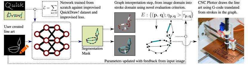
Figure 1: Left to Right. An artist drawing; digital copy of the drawing; segmented version; drawing by a cnc plotter.

Line is a fundamental building block in art form, and so has been emphasised by pioneers of historical art movements led by the likes of Picasso, Paul Klee, Kandinsky and Piet Mondrian in the past. In modern times drawing as an activity has been studied in the context of problem solving in a design process, while sampling mostly over line art[19, 20].

There is one question that forms the under-current of our investigation here,

If I provide any line drawing to a robot, how can I teach it to look at it, and draw the same on a paper using a pen.

This is a different challenge that has to the best of our knowledge not been addressed previously. There are vectorization based methods in Computer Graphics that aim to convert an input sketch into strokes. However, these would lose salient stroke information and would not preserve the line drawing (refer § 5.5). Other approaches aim to parse sketch into semantic segments. Again, this would not be useful for obtaining stroke information. In contrast to these, we aim to replicate the line drawing by converting an input raster line drawing image into a set of strokes (refer § 4) and the corresponding instructions (refer § 4.4) that can be used by an automated system. To obtain this, we present an approach different from the popular vectorization models [1, 17], the segmentation models [14, 8], the interesting developments of the drawing robots [4, 18] and further present its applicability.

We treat this problem as a special case of vectorization, by learning a function to map a line drawing from image domain to a graph structure. To this effect, we deploy, as a prior step in the pipeline, an image to image translation to facilitate the inference, using a deep segmentation neural network. There is also a post process step involved, to retrieve a sequence of strokes from the graph structure. This is further translated to gcode to input to a cnc plotter (refer § 4.4), or used directly by factory software to compute trajectory for a robotic arm.

We propose a novel U-Net based deep neural network (dnn) to implement the image to image translation, trained over a novel dataset built upon the Quick-draw dataset [6], and through a tailor-made training objective. The novelty in the dataset lies in generating on the fly, the segmentation true labels.

We propose a simple yet effective method, to infer the strokes as a graph data-structure, from the image domain. We utilise the segmentation of the image into corners channel, which for most practical cases have one to one correspondence with vertices of the graph, and lines, that show a similar behaviour of edges. The inference is made using an iterative update to a parametrized filter criterion, that selects a subset of the edges as graph proposal after every update.

To extract stroke sequences from the graph structure, we effectively utilise a recursive approach and illustrate the utility using two devices, namely cnc plotter, and a robotic arm.

To conclude through this paper we make the following main contributions:

• Propose a multistage pipeline, for segmentation, and graph interpretation;

• Novel architecture for the deep segmentation network;

• Annotated dataset for training the network;

• Improvised loss function as the training objective; and

• Feedback based iterative update to infer graph structure from image domain.

2 RELEVANT WORKS

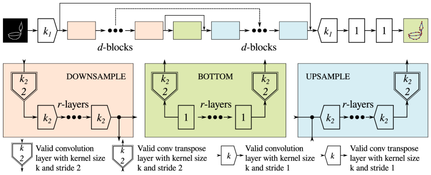
Figure 2: Reinterpretation of the U-Net architecture with modular blocks for downsampling, upsampling and bottom.

Research in robotics has seen some recent developments, while trying to create a drawing robot. Paul, the robotic arm, was trained to sketch a portrait, with inherent inputs from an artist, while deploying a stack of classical vision methods into their pipeline [18]. More recently,  [4, 3] investigated whether a similar feat can be achieved through a quad rotor, with the aim of “applying ink to paper with aerial robots.” Their contributions include computing a stipple pattern for an image, a greedy path planning, a model for strategically replacing ink, and a technique for dynamically adjusting future stipples based on past errors. Primarily, such efforts are based on space filling exercise, and focus on the control systems, rather than the accuracy of the input image. Our investigation deals more with capturing the line nature of artwork, and is a different exercise altogether.

Robots with high quality manipulators [16] have been used to draw line based art on uneven surface(s), exploiting the availability of impedance control. Earlier, Fu et al. [2] illustrated an effective use of graph minimisation over hand crafted features to predict a reasonable ordering of given strokes. However, these methods rely on vector input. We on the other hand propose a pipeline that reads from a grayscale image.

Sketch vectorization is very close to the graph structured learning part of our pipeline, but it has its own set of inherent problems [17]. Two specific approaches include skeleton based methods, that have to deal with corner artefacts, and contour based methods, that deal with problems related to one-to-one correspondences. Recent developments deal with noise removal and Favreau et.al. [1] in particular, investigate a higher order problem of fidelity vs simplicity of the method. Inherent to these approaches is the loss of information from the image domain in order to mitigate the basic problems. We propose to use segmentation techniques which are comparatively better at preserve the information as shown further in § 5.5.

Segmentation and labelling of sketches has been subject to profound research in graphics and vision. Schneider et al. [13] had successfully used an ensemble of Gaussian Mixture Models and Support Vector Machines with Fisher Vectors as distance metric to discriminate strokes; Further, it was illustrated that use of Conditional Random Fields over a relationship graph described by proximity and enclosure between the strokes, performs well in assigning semantic labels to strokes [14]. The classical methods use hard coded features like SIFT, that was used here, as the basic building block for learning algorithms.

Recently, convolutional neural networks have been proven to be highly effective in classifying segmented strokes as given labels [24]. Li et al. [9] have illustrated the effectiveness of U-Net based deep neural network architecture in the context of semantic segmentation, with the help of 3D objects dataset. The problems involving semantic segmentation whether used in classical context or with the deep learning based methods, target a higher level problem, namely semantics. We formulate our problem at a much lower level, by distinguishing corners from lines. Some problems also exploit the characteristics of dataset, for example data synthesised out of 3D objects, used by Li et al. [9], has a much stronger sense of enclosure, which are not necessarily true for the hand drawn counterparts, that form our dataset.

Sequence to sequence translation using deep learning methods have shown to be successfully deployed both as a discriminative model [22] as well as a generative model in the context of sketch segmentation [8]. The generative model has been used to reconstruct a sketched symbol. Sequences do make sense to work in stroke domain, where a sequence of vector input is available to begin with. Our work deals with an image as in input.

3 PIPELINE

The pipeline as shown in Fig. 1 can be split to three significant parts, namely

Image to Image Translation

The first part takes the raw sketch, a grayscale image as an input, and translates it into a segmentation mask, one for each label, which in our case are background, corners, and lines.

We implement this using a dnn, a variant of U-Net, that avoids cropping the images, and retains the valid convolution operations. This has been further detailed out in § 4.1 and § 4.2.

Graph Interpretation

The second part uses the segmentation channels of lines and corners as input and infers a graph structure, so that its vertices of the graph represent the cusp or end points, and its edges represent the curve drawn between them.

This is implemented using three parts; first is the inference of vertices, using connected component analysis of corners channel; second is a plausibility score of a given pair of vertices, evaluated using the lines channel; and finally a filter criterion based on a per edge threshold, that gets iteratively updated using feedback from the input image. This has further been detailed out in § 4.3.

Utility

The last part takes the graph structure and partitions into a sequence of strokes using a recursive approach. We further detail out the algorithm in § 4.4.

4 METHODOLOGY

4.1 Discovering the segmentation network

U-Net, proposed by Ronnenerger [12], was an extension of fully convolutional network [15, 10], and was shown to be highly effective in the context of biomedical segmentation. Compared to the FCN, U-Net proposed a symmetric architecture, to propagate the skip connections, within the convolutional network. The effectiveness in the context of semantic segmentation was also shown by Li et al. [9]

Additionally, since downsample/upsample is followed by valid convolutions, U-Net forwards only a crop of the activations as a skip connection. Consequently, the output of the vanilla U-Net produces an output image with size smaller than that of the input image, $H_{\mathrm{out}},W_{\mathrm{out}}<H_{\mathrm{in}},W_{\mathrm{in}}$. As a counter measure, the training and test images were augmented by tiled repetition at borders, for the vanilla U-Net.

We on the other hand create an exact mirror of operations in the U-Net architecture, i.e. downsampling is followed by valid convolutions and upsampling follows valid transpose convolutions. This eliminates the need for a tiling-based augmentation, and further gives way to nice convolution arithmetic.

Yu et.al [23] observed that in the context of sketches, the network is highly sensitive to the size of “first layer filters”, the “larger” the better. Although they used a kernel size of $(15\times{}15)$ for the first layer, we found that a size as low as $7\times{}7$ is effective in our case.

Another notable difference, inspired by Radford et. al’s observations  [11], has been in the downsampling and upsampling operations. U-Net uses “$2\times 2$ max pooling operation with stride 2 for downsampling” [and a corresponding upsampling strategy.] We have, on the other hand, used valid strided convolutions for downlasmpling, and valid strided transpose convolutions for up-sampling.

Our network, as shown in the Fig. 2 is parameterised with a 4-tuple,$(k_{1}\,k_{2}\,d\,r)$, where

• $k_{1}$ is the kernel $(k_{1}\times k_{1})$ of the first convolution layer.

• $k_{2}$ is the common kernel $(k_{2}\times k_{2})$ of all subsequent layers.

• $d$ is the depth of the U-Net, that is to say number of times to downsample during the contracting phase.

• $r$ is the number of horizontal layers along each depth level

4.2 Training Objective

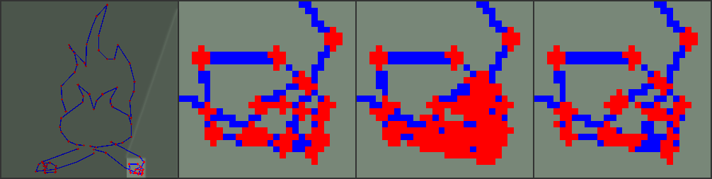
Figure 3: Effect of the change in weights for cross entropy loss. Left to Right. true labels highlighting selected area; blown up version of selected area in true labels; prediction in selected area using $\omega(\ell(\mathbf{x}))$; using max weights.

We started with the standard, weighted softmax cross entropy loss, as in the case of U-Net. For each pixel in the image, $\mathbf{x}\in\Omega;\Omega\subset\mathbb{Z}^{2}$, if the network activation corresponding to a given label $i$, be expressed as, $a_{i}(\mathbf{x});\,\,0<i\leqslant K$, we express the predicted probability of the label $i$, as the softmax of the activation, $p_{i}(\mathbf{x})=\mathrm{exp}(a_{i}(\mathbf{x}))/\sum_{j}^{K}\mathrm{exp}(a_{j}(\mathbf{x}))$. We want $p_{\ell(\mathbf{x})}\approx 1$ and $p_{i}(\mathbf{x})\approx 0;i\neq\ell(\mathbf{x})$ for the true label $\ell(\mathbf{x})$. So we penalise it against the weighted cross entropy, as follows:

$$\mathcal{L} =\sum_{\mathbf{x}\in\Omega}w(\mathbf{x})\log(p_{\ell(\mathbf{x})}(\mathbf{x}))$$ (1)

where $w(\mathbf{x})$ represents the weight map; which was initialised inversely proportional to class frequencies, $w(\mathbf{x})~{}\leftarrow~{}\omega(\ell(\mathbf{x}));~{}\omega:\Lambda\to\mathbb{R}$, where $\Lambda$ is the set of labels.

Further, we investigated a variant using max weights, $w(\mathbf{x})\leftarrow\omega(\max(\ell(\mathbf{x}),\rho(\mathbf{x})))$, where $\rho(\mathbf{x})$ is the predicted label. This significantly improves the result, as shown in Fig. 3. Even the prediction of very complicated structures resembles the true distribution.

4.3 Graph Interpretation

There are two key observations in interpreting the graph $G(V,E)$ representing the strokes, from a segmentation mask. Firstly, each corner is a set of strongly connected components in the channel, so we collect their centroids into the set of vertices, $V:\{\mathrm{centroid}(i);0<i\leqslant{}N\};V\subset\mathbb{R}^{2}$, where N is the number of connected components in the corners channel.

Secondly, along the line connecting centroids there is a peak response from lines channel, $Y_{\mathrm{lines}}$. We define a plausibility score, $\eta_{\mathbf{p},\mathbf{q}}$ of an edge between an arbitrary pair of vertices, $\mathbf{p},\mathbf{q}\in V;\mathbf{p}\neq\mathbf{q}$, as the average value of the lines channel masked by a region of interest (roi) $M$ between them. $M$ is defined as a narrow rectangular region, of width $\beta$ centred along the line segment $\overline{\mathbf{pq}}$. We define a per-pair, threshold parameter $\tau_{\mathbf{p},\mathbf{q}}$ based filter criterion, $C_{\mathbf{p},\mathbf{q}}$ as,

$$C_{\mathbf{p},\mathbf{q}} =\mathbf{I}\left[\eta_{\mathbf{p},\mathbf{q}}>\tau_{\mathbf{p},\mathbf{q}}\right]$$ (2)

$$\eta_{\mathbf{p},\mathbf{q}} =\frac{1}{|M|}\sum_{\mathbf{x}\in M}Y_{\mathrm{lines}}(\mathbf{x})$$

where, $\mathbf{I}$ is the indicator function.

Our experiments reveal that the threshold parameter varies with vertex pairs. We adapt $\tau_{\mathbf{p},\mathbf{q}}$, using a feedback loop, triggered by analysing the difference between the rendered strokes and the input image, using connected component analysis. The blobs thus obtained are characterised as a) absent blobs, that are present in input, but not rendered, $\mathbb{B^{+}}:\{\textrm{bounding box}\mathrel{}\forall\mathrel{}\textrm{absent blobs}\}$; and b) superfluous blobs, that are rendered, but not present in input, $\mathbb{B^{-}}:\{\textrm{bounding box}\mathrel{}\forall\mathrel{}\textrm{superfluous blobs}\}$. We do an iterative update of threshold parameter for all pairs of vertices as:

$$\tau^{i+1}_{\mathbf{p},\mathbf{q}} =\tau^{i}_{\mathbf{p},\mathbf{q}}(1+\lambda\,\delta_{\mathbf{p},\mathbf{q}})$$ (3)

$$\delta_{\mathbf{p},\mathbf{q}} =\begin{cases}-1,&\text{if}\mathrel{}\exists\mathrel{}i\mathrel{}\textrm{st.}\mathrel{}(\mathbf{p},\mathbf{q})\mathrel{}\textrm{inside}\mathrel{}B^{+}_{i}\in\mathbb{B^{+}};\\ 1,&\text{if}\mathrel{}\exists\mathrel{}j\mathrel{}\textrm{st.}\mathrel{}(\mathbf{p},\mathbf{q})\mathrel{}\text{inside}\mathrel{}B^{-}_{j}\in\mathbb{B^{-}};\\ 0,&\textrm{otherwise}\end{cases}$$

where $\lambda$ is an update hyperparameter.

4.4 Strokes and Gcode

In order to compute the strokes, we follow a recursive approach, so that every edge that is traversed is popped out of the graph, and revisiting the vertex is allowed. See Algorithms 1, 2.

Algorithm 1 Get_Sequence Recursive Procedure for generating Sequence of a Stroke

1:procedure Get_Sequence(A,u,S,strokes_cnt)
$\triangleright$ A is an adjacency list for N vertices. S is a list of strokes. strokes_cnt keeps track of total number of strokes. pop_edge(u,w) removes the edge (u,w) from the graph. A[u].get_vertex() returns a vertex from adjacency list of u.

2:

3:     If $A[u]$ $==$ $\mathbf{Null}$

4:         return

5:     $w\leftarrow$ $A[u]\textbf{.get\_vertex()}$

6:     pop_edge(u,w)

7:     S[strokes_cnt].append(w)

8:     $\textsc{Get\_Sequence}(A,w,S,\mathit{strokes\_cnt})$

9:end procedure

Algorithm 2 Strokes_Gen Procedure for generating strokes from undirected graph

1:procedure Strokes_Gen(A)
$\triangleright$ Strokes_Gen procedure called with adjacency list A

2:

3:     $\mathrm{strokes\_cnt}=0$

4:     while ($A[v]\hskip 2.84544pt!\hskip 2.84544pt\mathbf{Null}\hskip 5.69046pt\forall v$) do

5:         S[strokes_cnt].append(v)

6:         $u\leftarrow$ $A[v]\textbf{.get\_vertex()}$

7:         S[strokes_cnt].append(u)

8:         pop_edge(v,u)

9:         $\textsc{Get\_Sequence}(A,u,S,\mathit{strokes\_cnt})$

10:         $\text{strokes\_cnt}\leftarrow{}\mathrm{strokes\_cnt}+1$

11:     end while

12:end procedure

The strokes are finally translated to gcode using a simple translation method. Issue for each stroke in the set, the following commands sequentially,

• push first vertex, (Xff.ff Yff.ff),

• engage (G01 Z0),

• push rest of the vertices (Xff.ff Yff.ff ...), and

• disengage (G00 Z-5)

There are two caveats to remember here. Firstly, to disengage (G00 Z-5) at the start. And secondly to rescale the coordinates as per machine, for example, Z-5 pertains to 5 mm away from work, which in case of cm units or inch units, should be scaled by an appropriate factor.

A very similar method is used to render to an SVG Path [21], where each stroke is a series of 2D points, expressed in XML as, <path d="M x0 y0 L x1 y1 [L x y ...]" /> This is input to the robotic arm to draw on paper.

5 EXPERIMENTATION

5.1 Dataset

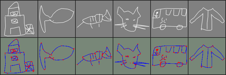
Figure 4: Top. Samples from the Quick-draw dataset; Bottom. Rendered true labels.

We use the Quick-draw dataset [6] for the basic line art. The sketches are available to us in the form of a list of strokes, and each stroke is a sequence of points. The data is normalised, centred to canvas, and re-scaled to accommodate for stroke width, before being rasterised, using drawing functions, in order to synthesise the input image, $X;X~{}\in~{}\mathbb{R}^{s\times{}s}$.

For the purpose of segmentation, an active pixel is either identified as a corner (node in the graph), a connecting line, or the background; i.e. $K=3$ classes. We compute the intersections using the vector data from Quick-draw, and append them to the accumulated set of corners, so that they are rasterised as $Y_{\mathrm{corners}}$. The difference operation, with respect to the input, gives us the lines channel, $Y_{\mathrm{lines}}=X-Y_{\mathrm{corners}}$. Everything else is the background, $Y_{\mathrm{bg}}=1-(Y_{\mathrm{corners}}+Y_{\mathrm{lines}})$. Thus, we obtain the true labels, $Y~{}\in~{}\mathbb{R}^{K\times{}s\times{}s}$. A glimpse of the dataset can be seen in Fig. 4.

We created a set of $\sim{}65k$ samples for the training, and $\sim{}10k$ samples for testing; each sample being a pair of images, namely the input image and the true labels. We will make it available to public domain after acceptance of this paper.

5.2 Segmentation

Figure 5: Validation Accuracy (iou’s) using models check-pointed during the training. (x-axis:Training epochs, y-axis:iou)

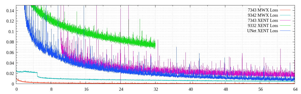
Figure 6: Validation Loss using models check-pointed during the training. (x-axis:Training epochs, y-axis:Loss)

We experimented with various combinations of network architectures, and training objectives, to find a suitable segmentation network. The most promising ones that have been presented here are: a) Net $(9\,3\,2\,2)$ with cross-entropy loss (xent); b) Net $(9\,3\,3\,2)$ with xent; c) Net $(7\,3\,4\,3)$ with xent; d) Net $(7\,3\,4\,3)$ with max-weighted cross-entropy loss (mwx). (For network nomenclature, refer § 4.1 and Fig. 2.) Additionally, we also trained a variant of vanilla U-Net with xent, where we replaced ‘valid’ convolutions with padded-convolutions to obtain consistent image sizes on our dataset. As per our nomenclature, the vanilla U-Net corresponds to $(3\,3\,4\,2)$ architecture. The optimiser used was RMSProp [7], with $\beta=0.9$.

The validation accuracy and losses during the training are reported in the Fig. 5,6. The x-axis represents number of epochs of training in both the figures. The y-axis represents the average iou (“intersection over union”) in Fig. 5, and in Fig. 6, it represents the average loss. The model was evaluated using validation set. We can see that net $(7\,3\,4\,3)$ with mwx stabilises fastest and promises the most accurate results. A quantitative summary of our evaluation over the test set, is shown in the Table 1. Here also we see a similar trend, as expected, i.e. $(7\,3\,4\,3)$ with mwx is a winner by far. Qualitatively, the implication of a better segmentation is most prominently visible in fairly complicated cases, e.g. Fig. 3. This improvement in the results is attributed to the design of max-weighted cross entropy loss (refer § 4.2).

Table 1: Accuracy measure of segmentation networks

Architecture	Loss Function	iou $(\%)$
Net $(7\,3\,4\,3)$	mwx	98.02%
Net $(9\,3\,4\,2)$	mwx	91.24%
Net $(7\,3\,4\,3)$	xent	92.57%
Net $(9\,3\,3\,2)$	xent	75.09%
Vanilla U-Net	xent	94.23%

5.3 Graph

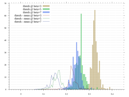
Figure 7: Histogram of approximate plausibility threshold $\widehat{\tau}$ and its distance from the average value of corresponding plausibility score $\overline{\eta}$ for different values of mask widths $\beta$. (x-axis:Threshold values)

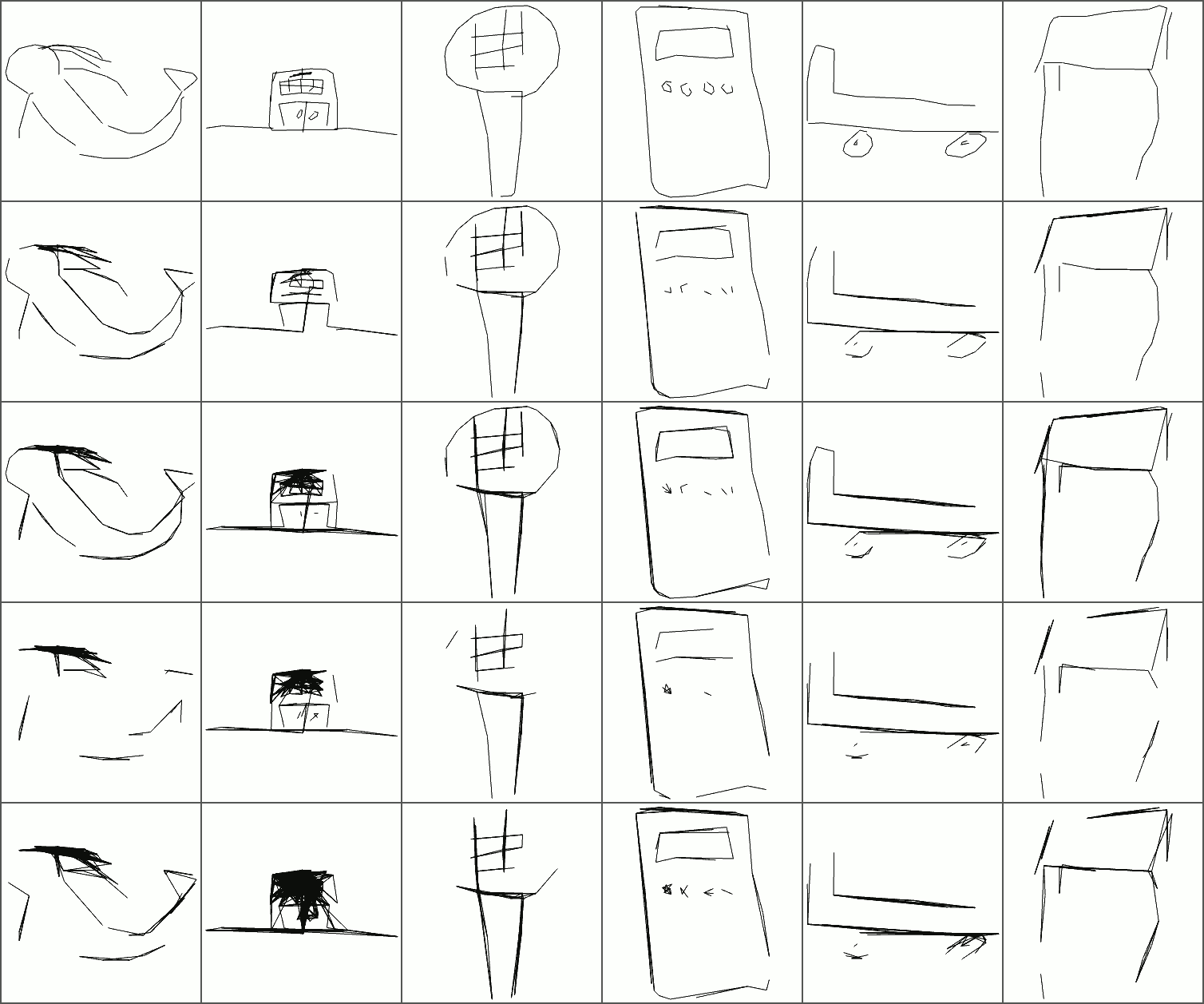
Figure 8: The top row shows the input. The subsequent rows show reconstruction using a graph interpreted from segmentation mask, with values of mask width and threshold $(\beta,\tau)$ set as (2, 0.3), (3, 0.22), (5, 0.2), (7, 0.15) respectively downwards.

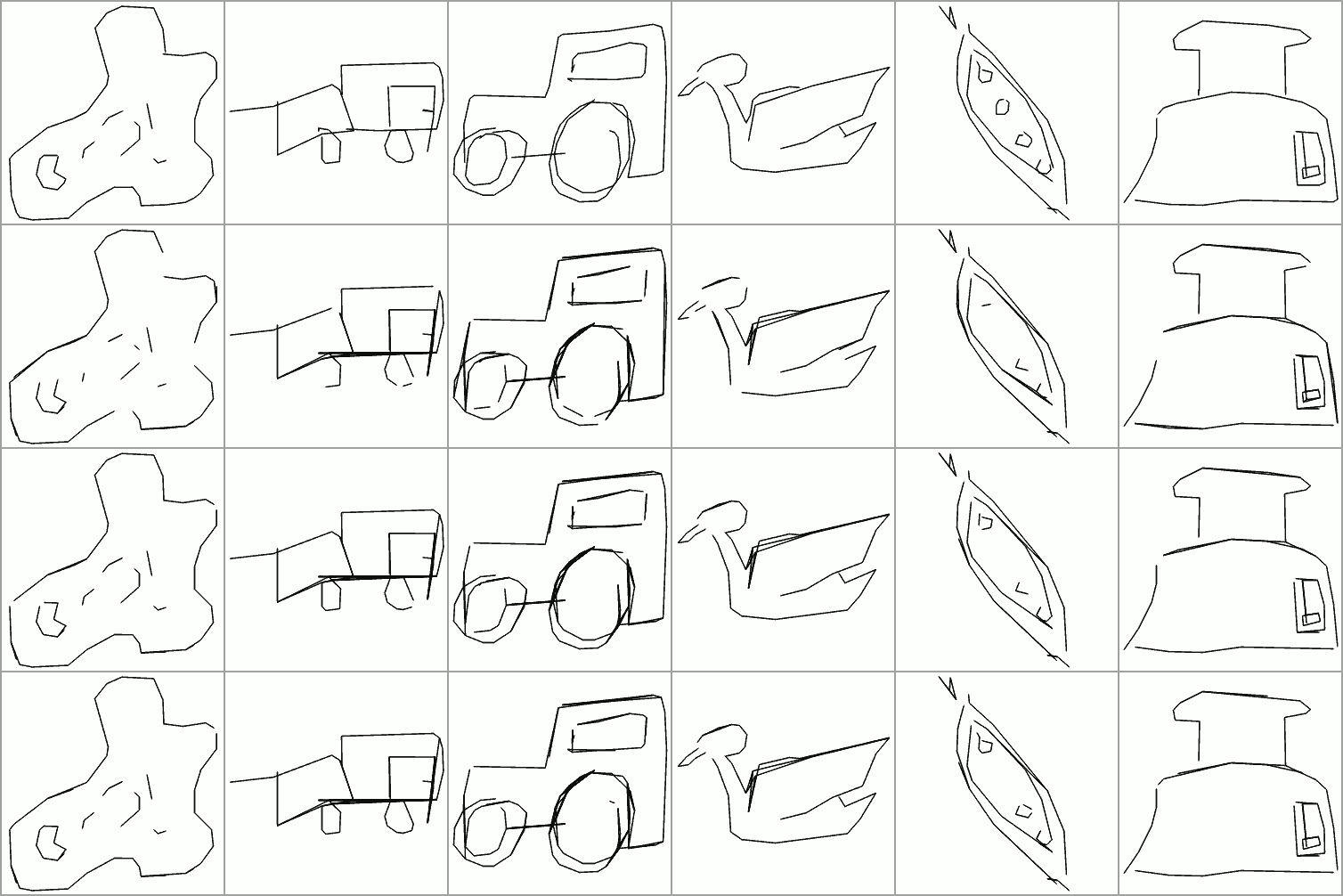
Figure 9: The results of feedback loop in graph interpretation. Rows top to bottom. the input image; naïve graph interpretation; interpretation after $N=5$ updates; and after $N=10$ updates.

For graph interpretation, we analysed the distribution of plausibility score over the test dataset, as defined in Eq. 2, with a view, that there should be a clear separation between the pairs of centroids containing edges and the pairs without edges. To investigate this, we experimented with three values of mask width parameter $\beta\in\{3,\,5,\,7\}$. For a given image in the dataset, we already know the number of lines, which we leverage to find the approximate threshold $\widehat{\tau}$, by sorting the plausibility scores $\eta_{\mathbf{p},\,\mathbf{q}}$ in reverse and truncating. We smoothen out the value of $\widehat{\tau}$ by averaging over a neighbourhood of size $k=3$. Further, we collect the values of $\widehat{\tau}$ and average plausibility score $\overline{\eta}$ for selected values of $\beta$, across the images in test set. The histograms for $\widehat{\tau}$ in Fig 7 show a single prominent peak and light tail; and the histograms of $\widehat{\tau}-\overline{\eta}$ show that there is a comfortable margin between $\widehat{\tau}$ and $\tau$, which implies that, for our distribution from Quick-draw dataset, there indeed is a clear separation between the pairs of centroids containing edges and the pairs without edges.

Further we qualitatively tested the method with values of mask-width $\beta$ and a fixed plausibility threshold of $\tau$ set to $(2,\,0.3)$, $(3,\,0.22)$, $(5,\,0.2)$ and $(7,\,0.15)$ respectively. The results are shown in Fig. 8. We see that a fixed value of threshold is not able to capture the edges based on the plausibility score.

Thereafter, we tested the adaptive update method, designed in Eq. 3, with heuristically set parameters: mask width $\beta=1.8$, initial plausibility threshold $\tau^{(0)}=0.35$, update rate $\lambda=0.05$. Typically, we found satisfactory results with $N=10$ updates. In Fig. 9, the second row is a rendering of graph interpreted with $\tau^{(0)}$, and has missed a few strokes. In almost all the cases after $N=10$ updates (bottom row) the missing strokes have been fully recovered!

5.4 Application

We tested the results for application with two robots. First is a traditional cnc milling machine “emco Concept Mill 250,” where we used pen as a tool to plot over a plane surface. This machine accepts gcode as input. Second is a modern robotic arm “Dobot Magician Robotic Arm,” that holds a pen to draw on paper. This machine accepts line drawings in svg format, such that each stroke is defined as a path element. The method of post processing the list of strokes to either create gcode for cnc plotter or create svg for a robotic arm is detailed out in § 4.4. For practical purposes, we fixed the drawings in either case to be bounded within a box of size $64\mathrm{mm}\times 64\mathrm{mm}$ and set the origin at $(25\mathrm{mm},\,25\mathrm{mm})$ Fig. 11 shows a still photograph of the robots in action. Reader is encouraged to watch the supplementary video for a better demonstration.

5.5 Generalisation

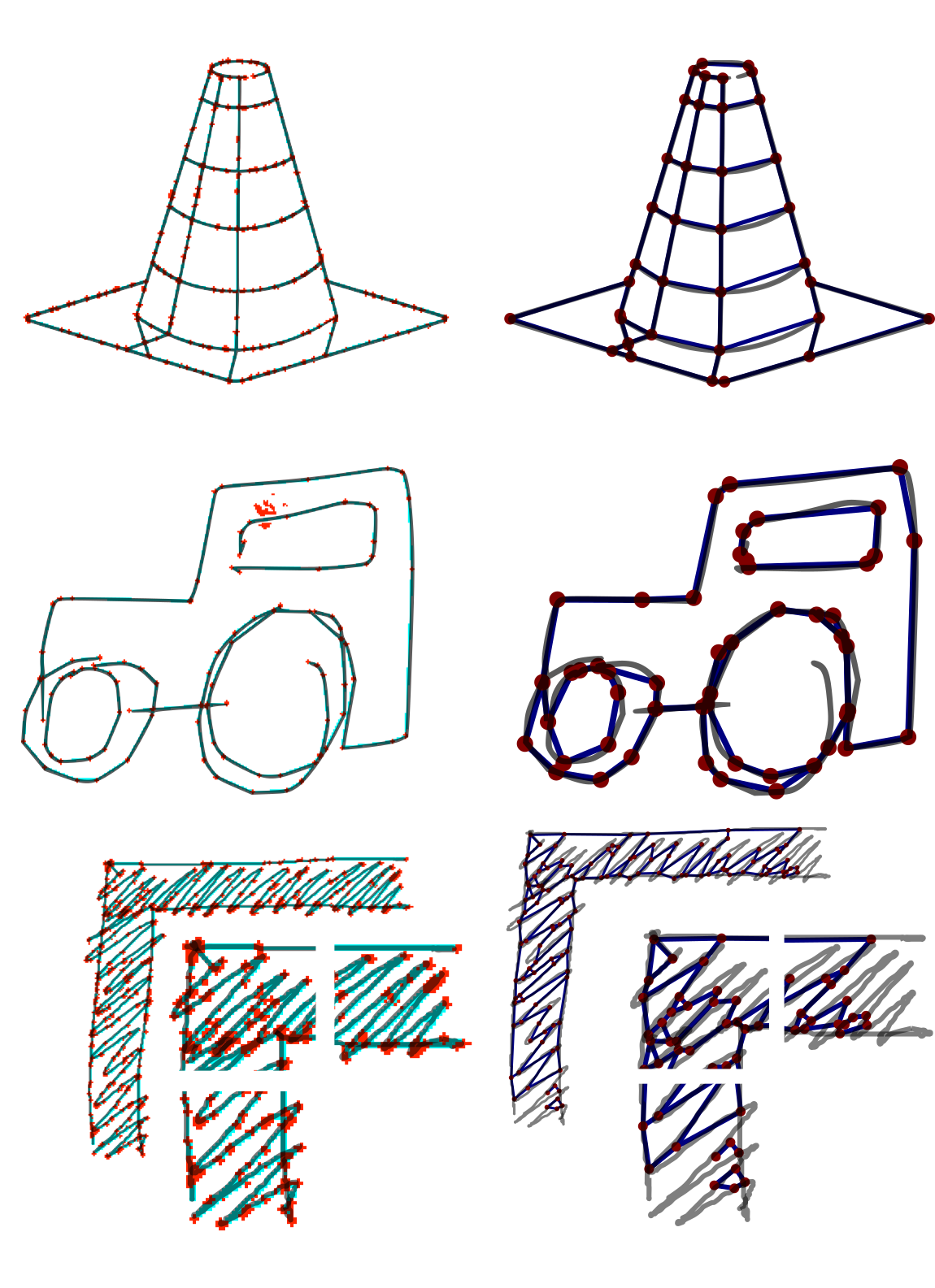
Figure 10: Comparison of our segmentation (left column) against Favreau’s vectorization (right column). Top to Bottom. A simple line sketch from Favreau’s examples; A simple line sketch from Quick-draw dataset; A complicated hatch pattern with zoomed in details.

A deep learning based method is generally preferred for it generalises well. Here we qualitatively inspect our model against Favreau et al.’s vectorization method[1] to line drawing vectorization, using three different samples, namely a simple sketch from their samples; a simple sketch from Quick-draw; and a complicated sketch, representing a hatch pattern, commonly used to represent walls in architectural graphics. In Fig. 10, we see that our method produces satisfactory segmentation on both the simple cases, and also gracefully degrades its performance in the complicated case; whereas, the latter method, compromises on details, e.g. few open strokes near the wheels of the automobile, and thus fails miserably on the complicated task of vectorizing a hatch pattern, missing out several details.

6 CONCLUSION

We have portrayed an alternate method for a drawing robot in the context of line drawings, which maps image domain to a graph structure that represents the original image, and retrieve a set of actionable sequences.

There is definitely, a scope of improvement here. We see the following points to be most significant,

• The segmentation model is highly sensitive to noise, and similar phenomenon has been observed in the context of deep learning by Goodfellow et.al [5]. This problem is subject of contemporary research.

• Graph interpretation method is sensitive to initial choice of threshold parameter $\tau$ and the update hyperparameter $\lambda$, refer eq. 3.

The pipeline proposed by us is a multi utility technique, the use of which we have portrayed through a CNC machine as well as through a robotic arm as shown in Fig. 11

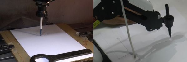
Figure 11: Demonstration of the applicability of our output using two different machines, namely, the cnc plotter in the left, and the robotic arm in the right.

References

- [1] J.-D. Favreau, F. Lafarge, and A. Bousseau. Fidelity vs. simplicity: A global approach to line drawing vectorization. ACM Transactions on Graphics (TOG), 35(4):120, 2016.
- [2] H. Fu, S. Zhou, L. Liu, and N. J. Mitra. Animated construction of line drawings. In Proceedings of the 2011 SIGGRAPH Asia Conference on - SA ’11, page 1, Hong Kong, China, 2011. ACM Press.
- [3] B. Galea, E. Kia, N. Aird, and P. G. Kry. Stippling with aerial robots. In Proceedings of the Joint Symposium on Computational Aesthetics and Sketch Based Interfaces and Modeling and Non-Photorealistic Animation and Rendering, Expressive '16, pages 125–134. Eurographics Association, 2016.
- [4] B. Galea and P. G. Kry. Tethered flight control of a small quadrotor robot for stippling. In 2017 IEEE/RSJ International Conference on Intelligent Robots and Systems (IROS), pages 1713–1718, Vancouver, BC, Sept. 2017. IEEE.
- [5] I. J. Goodfellow, J. Shlens, and C. Szegedy. Explaining and harnessing adversarial examples. arXiv preprint arXiv:1412.6572, 2014.
- [6] D. Ha and D. Eck. A Neural Representation of Sketch Drawings. arXiv:1704.03477 [cs, stat], Apr. 2017.
- [7] G. E. Hinton, N. Srivastava, and K. Swersky. Overview of mini-batch gradient descent.
- [8] K. Kaiyrbekov and M. Sezgin. Stroke-based sketched symbol reconstruction and segmentation. arXiv:1901.03427 [cs], Jan. 2019.
- [9] L. Li, H. Fu, and C.-L. Tai. Fast Sketch Segmentation and Labeling with Deep Learning. IEEE Computer Graphics and Applications, pages 1–1, 2018.
- [10] J. Long, E. Shelhamer, and T. Darrell. Fully Convolutional Networks for Semantic Segmentation. In The IEEE Conference on Computer Vision and Pattern Recognition (CVPR), June 2015.
- [11] A. Radford, L. Metz, and S. Chintala. Unsupervised Representation Learning with Deep Convolutional Generative Adversarial Networks. arXiv:1511.06434 [cs], Nov. 2015.
- [12] O. Ronneberger, P. Fischer, and T. Brox. U-Net: Convolutional Networks for Biomedical Image Segmentation. arXiv:1505.04597 [cs], May 2015.
- [13] R. G. Schneider and T. Tuytelaars. Sketch classification and classification-driven analysis using Fisher vectors. ACM Trans. Graph., 33(6), Nov. 2014.
- [14] R. G. Schneider and T. Tuytelaars. Example-Based Sketch Segmentation and Labeling Using CRFs. ACM Trans. Graph., 35(5):151:1–151:9, July 2016.
- [15] E. Shelhamer, J. Long, and T. Darrell. Fully Convolutional Networks for Semantic Segmentation. IEEE Transactions on Pattern Analysis and Machine Intelligence, 39(4):640–651, Apr. 2017.
- [16] D. Song, T. Lee, and Y. J. Kim. Artistic Pen Drawing on an Arbitrary Surface Using an Impedance-Controlled Robot. In 2018 IEEE International Conference on Robotics and Automation (ICRA), pages 4085–4090, Brisbane, QLD, May 2018. IEEE.
- [17] K. Tombre and S. Tabbone. Vectorization in graphics recognition: To thin or not to thin. In Proceedings 15th International Conference on Pattern Recognition. ICPR-2000, volume 2, pages 91–96, Barcelona, Spain, 2000. IEEE Comput. Soc.
- [18] P. Tresset and F. Fol Leymarie. Portrait drawing by Paul the robot. Computers & Graphics, 37(5):348–363, Aug. 2013.
- [19] D. G. Ullman, S. Wood, and D. Craig. The importance of drawing in the mechanical design process. Computers & Graphics, 14(2):263–274, 1990.
- [20] W. Visser. The Cognitive Artifacts of Designing. CRC Press, 2006.
- [21] World Wide Web Consortium (W3C). Paths — SVG 2. https://www.w3.org/TR/SVG/paths.html, Oct. 2018.
- [22] X. Wu, Y. Qi, J. Liu, and J. Yang. Sketchsegnet: A Rnn Model for Labeling Sketch Strokes. In 2018 IEEE 28th International Workshop on Machine Learning for Signal Processing (MLSP), pages 1–6, Sept. 2018.
- [23] Q. Yu, Y. Yang, F. Liu, Y.-Z. Song, T. Xiang, and T. M. Hospedales. Sketch-a-Net: A Deep Neural Network that Beats Humans. International Journal of Computer Vision, 122(3):411–425, May 2017.
- [24] X. Zhu, Y. Xiao, and Y. Zheng. Part-Level Sketch Segmentation and Labeling Using Dual-CNN. In L. Cheng, A. C. S. Leung, and S. Ozawa, editors, Neural Information Processing, volume 11301, pages 374–384. Springer International Publishing, Cham, 2018.