Abstract

In this paper we re-investigate the model of the anti-de Sitter gravity coupled to Maxwell and charged scalar fields, which has been studied as the gravitational dual to a superconductor for a long time since the famous work [Phys. Rev. Lett.  101, 031601 (2008)]. By numerical method, we present a novel family of solutions of holographical superconductor with excited states, and find there exists a lower critical temperature in the corresponding excited state. Moreover, we study the condensate and conductivity in the excited states. It is very interesting that the conductivity $\sigma$ of each excited state has an additional pole in $\text{Im}[\sigma]$ and a delta function in $\text{Re}[\sigma]$ arising at the low temperature inside the gap, which is just the evidence of the existence of excited states.

1 Introduction

In condensed matter physics, there is still no consensus on the mechanism of high temperature superconductivity. Over the past decade, the AdS/CFT correspondence [1, 2, 3] is one of the most important results from string theory, which establishes the relationship between the strongly correlated field on the boundary and a weak gravity theory in one higher-dimensional bulk spacetime. In the past ten years, the AdS/CFT correspondence has provided a novel way to study condensed matter theory, and received a great deal of attention. In the seminal papers [4, 5, 6], the authors investigated the model of a complex scalar field coupled to a $U(1)$ gauge field in a ($3+1$)-dimensional Schwarzschild-AdS black hole and found that due to the $U(1)$ symmetry breaking below the critical temperature $T_{c}$, the condensate of the scalar field could be interpreted as the Cooper pair-like superconductor condensate. Moreover, there exists a gap in the optical conductivity of the superconducting state, and the value of the gap is close to the value of a high temperature superconductor. Thus, this model can be regarded as the dual explanation to the high temperature superconductor. When replacing the scalar field with other matter fields, one can also obtain the condensate of matter fields corresponding to various kinds of holographic superconductors. For example, holographic d-wave model was constructed by introducing a symmetric, traceless second-rank tensor coupled to a $U(1)$ gauge field in the bulk [7, 8, 9]. With the SU(2) Yang-Mills field coupled to gravity, the holographic p-wave model has also been discussed in [10]. Two alternative holographic realizations of p-wave superconductivity could arise from the condensate of a two-form field [11] and a complex, massive vector field with $U(1)$ charge [12, 13], respectively. The model of holographic superconductor can also be extended to study the holographic Josephson junction [14, 15, 16, 17, 18, 19, 20, 21, 22, 23, 24, 25, 26], which is made up of two superconductor materials with weak link barrier [27]. A top-down construction of holographic superconductor from superstring theory was discussed in [28], and a similar construction using an M-theory truncation was proposed in [29, 30]. For reviews of holographic superconductors, see [31, 32, 33, 34].

Until now, lots of work of holographic superconductor were investigated in the ground state, that is, the scalar field can keep sign along the radial direction. It is well-known that the excited states could have some nodes along the radial direction, where the value of the scalar field could change the sign. On the other hand, it is easy to see in quantum theory that the bound states with given angular momentum and other quantum numbers similarly could form towers of states known as radial excitations with otherwise identical quantum numbers. Especially, holographic phenomenological models [37, 38] have the potential to provide a better understanding of strongly interacting systems of quarks and gluons, including the excited states of hadrons. These models are presently known as AdS/QCD. Furthermore, in the background of Schwarzschild black hole, holographic model of QCD could be extended to the finite temperature system [39], There are also many new progresses on the excited states of hadrons from holographic QCD, such as [40, 41, 42].

So, it is interesting to see whether there exist the solutions of holographic superconductor with excited states of the scalar field. In the present paper, we would like to numerically solve the Maxwell-Klein-Gordon system with the background of a four-dimensional Schwarzschild-AdS black hole and give a family of excited states of holographic superconductors with different critical temperatures. Moreover, we will also study the condensate and optical conductivity in the excited states of holographic superconductors.

The paper is organized as follows: in Sect. 2, we review the model of a $U(1)$ gauge field coupled with a charged scalar field in ($3+1$)-dimensional AdS spacetime and show a gravity dual model of holographic superconductor. We show the numerical results of the excited states and study the characteristics of the condensate and conductivity in Sect. 3. The conclusion and discussion are given in the last section.

2 Review of holographic superconductors

Let us introduce the model of a Maxwell field and a charged complex scalar field in the four-dimensional Einstein gravity spacetime with a negative cosmological constant. The bulk action reads

$$\mathcal{S}=\frac{1}{16\pi G}\int\mathrm{d}^{4}x\left[R+\frac{6}{\ell^{2}}-\frac{1}{4}F^{\mu\nu}F_{\mu\nu}-(\mathcal{D}_{\mu}\psi)(\mathcal{D}^{\mu}\psi)^{*}-m^{2}\psi\psi^{*}\right],$$ (2.1)

where $F_{\mu\nu}=\partial_{\mu}A_{\nu}-\partial_{\nu}A_{\mu}$ is the field strength of the $U(1)$ gauge field, and $\mathcal{D}_{\mu}=\nabla_{\mu}-iqA_{\mu}\psi$ is the gauge covariant derivative with respect to $A_{\mu}$. The constant $\ell$ is the AdS length scale, $m$ and $q$ are the mass and charge of the complex scalar field $\psi$, respectively. Due to the existence of Maxwell and complex scalar field, the strength of the backreaction of the matter fields on the spacetime metric could be tuned by the charge $q$. In order to see that how the effect of backreaction varies with the charge $q$, we could introduce the scaling transformations $A\rightarrow A/q$ and $\psi\rightarrow\psi/q$, and the Lagrangian density in Eq. (2.1) changes into

$$16\pi G\mathcal{L} = R+\frac{6}{\ell^{2}}+\kappa\left(-\frac{1}{4}F^{\mu\nu}F_{\mu\nu}-|\nabla\psi-iA\psi|^{2}-m^{2}\psi\psi^{*}\right),$$ (2.2)

with the constant $\kappa\equiv 1/q^{2}$. From the above, we can see that the value of the parameter $\kappa$ will decrease when $q$ increases, and the backreaction of matter fields on the spacetime metric could be ignored in the large $q\rightarrow\infty$ limit, which is also called as the probe limit. Here we adopt to the probe approximation. Thus, the following equations of the scalar and Maxwell fields can be derived from the Lagrangian density (2.2):

$$(\nabla_{\mu}-iA_{\mu})(\nabla^{\mu}-iA^{\mu})\psi-m^{2}\psi = 0,$$ (2.3)

$$\nabla_{\mu}F^{\mu\nu}-i[\psi^{\ast}(\nabla^{\nu}-iA^{\nu})\psi-\psi(\nabla^{\nu}+iA^{\nu})\psi^{\ast}] = 0.$$ (2.4)

In addition, with neglect of the backreaction of matter fields on the metric, the solution of Einstein equations is the well-known Schwarzschild anti-de Sitter black hole. The solution with a planar symmetric horizon can be written as follows

$$ds^{2}=-f(r)dt^{2}+\frac{dr^{2}}{f(r)}+r^{2}(dx^{2}+dy^{2}),$$ (2.5)

where $f(r)=\frac{r^{2}}{\ell^{2}}(1-r_{h}^{3}/r^{3})$, and $r_{h}$ is the radius of the black hole’s event horizon. The Hawking temperature is given by

$$T=\frac{1}{4\pi}\frac{df}{dr}\bigg{|}_{r=r_{h}}=\frac{3r_{h}}{4\pi\ell^{2}},$$ (2.6)

which can be regarded as the temperature of holographic superconductors.

In order to build a holographic model of holographic superconductors, one could introduce the following ansatz of matter fields:

$$A=\phi(r)dt,\;\;\;\;\;\psi=\psi(r).$$ (2.7)

With the above ansatz, the equations of motion for the scalar field $\psi(r)$ and electrical scalar potential $\phi(r)$ in the background of the Schwarzschild-AdS black hole are

$$\psi^{\prime\prime}+\left(\frac{f^{\prime}}{f}+\frac{2}{r}\right)\psi^{\prime}+\frac{\phi^{2}}{f^{2}}\psi-\frac{m^{2}}{\ell^{2}f}\psi = 0\,,$$ (2.8)

$$\phi^{\prime\prime}+\frac{2}{r}\phi^{\prime}-\frac{2\psi^{2}}{f}\phi = 0.$$ (2.9)

At the AdS boundary, the asymptotic behaviors of the functions $\psi(r)$ and $\phi(r)$ take the following forms

$$\psi = \frac{\psi^{(1)}}{r^{\Delta_{-}}}+\frac{\psi^{(2)}}{r^{\Delta_{+}}}+\cdots\,,$$ (2.10)

$$\phi = \mu-\frac{\rho}{r}+\cdots\,,$$ (2.11)

with

$$\Delta_{\pm}=\frac{3\pm\sqrt{9+4m^{2}}}{2},$$ (2.12)

where the constants $\mu$ and $\rho$ are the chemical potential and charge density in the dual field theory, respectively. According to AdS/CFT duality, $\psi^{(i)}(i=1,2)$ are the corresponding expectation values of the dual scalar operators $\mathcal{O}_{i}$, respectively. Note that in the four-dimensional spacetime the values of mass need to satisfy the Breitenlohner-Freedman (BF) bound of $m^{2}\geq-9/4$ [43]. In this paper, we will set $m^{2}=-2$ for simplify.

3 Numerical results

In this section, we will solve the above coupled equations (2.8) and (2.9) numerically. It is convenient to change the radial coordinate $r$ to the new radial coordinate $z=r_{h}/r$. For simplify, we set $\ell=1$ and $r_{h}=1$. Thus the inner and outer boundaries of the shell are fixed at $z=0$ and $z=1$, respectively. All numerical calculations are based on the spectral methods. Typical grids used have the sizes from $50$ to $300$ in the integration region $0\leq z\leq 1$. Our iterative process is the Newton-Raphson method, and the relative error for the numerical solutions in this work is estimated to be below $10^{-5}$.

In an approach based on the Newton-Raphson method, a good initial guess for the profile of the functions $\psi$ and $\phi$ is an essential condition for a successful implementation. To obtain numerically the ground state solution, one can use the profile of a constant as a initial guess for the function $\psi$. Meanwhile, for the $n$-th excited state case, one need choose a initial guess with $n$ nodes for the function $\psi$.

It is well-known that there exists a critical temperature $T_{c}$, above which there is no scalar condensate in the Schwarzschild-AdS black hole background, while for $T\leq T_{c}$, the scalar condensate begins to appear due to the spontaneously broken $U(1)$ gauge symmetry. Until now, only the ground state of holographic superconductor with a fixed critical temperature was found out, that is, the scalar field $\psi$ could keep sign along the radial direction. By numerically solving the same equations of motion with boundary conditions as the case of ground state, we could also obtain the solutions of the excited states, in which the value of the scalar field can change sign along the radial direction.

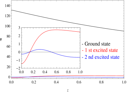
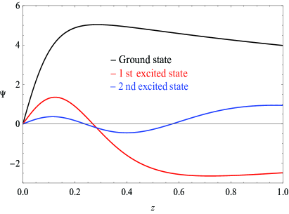
Figure 1: Left: The distribution of the scalar field $\psi$ as a function of $z$ coordinate with the chemical potential $\mu=12$ for the condensate $\langle{\mathcal{O}}_{1}\rangle$. Right: The distribution of the scalar field $\psi$ as a function of $z$ coordinate with $\mu=15$ for the condensate $\langle{\mathcal{O}}_{2}\rangle$. In both plots, the black, red and blue lines denote ground state, first and second states , respectively.

In Fig. 1, we show two kinds of typical results of the distribution of the scalar field $\psi$ as a function of $z$ for the condensates $\langle{\mathcal{O}}_{1}\rangle$ and $\langle{\mathcal{O}}_{2}\rangle$, respectively. The values of the chemical potential $\mu$ are equal to 12 (left panel) and 15 (right panel). In both plots, the black, red and blue lines denote ground state, first and second states, respectively. The inset in left panel shows the detail of the curves of the first and second excited states. From Fig. 1, we can see that the ground state has no nodes, and $n$-th excited state has exactly $n$ nodes, where the values of the scalar field are equal to zero. Moreover, the amplitude of $\psi$ deceases with higher excited states.

	$0$	$1$	$2$	$3$	$4$	$5$	$6$
$\langle{\mathcal{O}}_{1}\rangle$	1.120	6.494	11.701	16.898	22.094	27.290	32.486
$\langle{\mathcal{O}}_{2}\rangle$	4.064	9.188	14.357	19.538	24.725	29.915	35.107

Table 1: Critical chemical potential $\mu_{c}$ for the operators ${\mathcal{O}}_{1}$ and ${\mathcal{O}}_{2}$ from the ground state to sixth excited state.

In the table 1, we present the results of the critical chemical potential $\mu_{c}$ for the operators ${\mathcal{O}}_{1}$ and ${\mathcal{O}}_{2}$ from the ground state to sixth excited state. We can see that an excited state can be regarded as a new static solution of holographic superconductors that has a higher critical chemical potential than the ground state, that is, an excited state has a higher critical charge density $\rho_{c}$. Because the critical temperature is proportional to $\rho^{-1/2}_{c}$ in four-dimensional spacetime, the excited state has a lower critical temperature than the ground state. With the decrease of the temperature, the ground state first appears, and when the temperature is lower to the critical temperature of the first-excited state, the solutions of the first-excited state begin to appear. It is interesting to note that the difference of critical chemical potential $\mu_{c}$ between the consecutive states is about $5$ regardless of the condensates $\langle\mathcal{O}_{1}\rangle$ or $\langle\mathcal{O}_{2}\rangle$. The relation between $\mu_{c}$ and $n$ can be fitted as

$$\mu_{c}\approx\left\{\begin{array}[]{ll}5.217n+1.217\,,&\qquad\textrm{for}\;\;{\mathcal{O}}_{1},\\ 5.177n+4.026\,,&\qquad\textrm{for}\;\;{\mathcal{O}}_{2}.\end{array}\right.$$

3.1 Condensates

According to AdS/CFT duality, the expectation values of the condensate operator $\langle\mathcal{O}_{i}\rangle$ is dual to the scalar field $\psi^{(i)}$:

$$\langle{\mathcal{O}}_{i}\rangle=\sqrt{2}\psi^{(i)}\,,\quad i=1,2.$$ (3.13)

In Fig. 2, we show the condensate as a function of the temperature for the two operators ${\mathcal{O}}_{1}$ (left) and ${\mathcal{O}}_{2}$ (right) of excited states. In both plots, the black, red and blue lines denote ground state, first and second states, respectively. In the left panel, the condensate of ground state for the operator $\langle\mathcal{O}_{1}\rangle$ appears to diverge as the temperature $T\rightarrow 0$, which means the backreaction of the bulk metric can no longer be neglected. However, the condensate of excited states does not appear to diverge as $T\rightarrow 0$, and the condensate goes to a constant near zero temperature. Moreover, the condensate of an excited state is smaller than the ground state. Especially, we can see that the value of the condensate for the second excited state near zero temperature is very closed to that of the first excited state. We have calculated the condensate of zero temperature until the sixth excited state, and find that this value is about 4.4. In the right panel, the condensate of the ground state for the operator $\mathcal{O}_{2}$ appears to converge as the temperature $T\rightarrow 0$, and the condensate of an excited state is larger than the ground state.

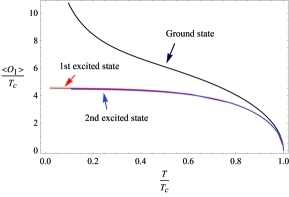
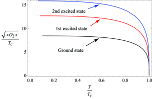
Figure 2: The condensate as a function of the temperature for the two operators ${\mathcal{O}}_{1}$ (left) and ${\mathcal{O}}_{2}$ (right) of excited states. In both plots, the black, red and blue lines denote ground state, first and second states, respectively.

When the temperature drops below the critical temperature $T_{c}$, the model of holographic superconductor has a second order phase transition from normal state to superconductor state. Moreover, there exists a square root behaviour near the critical point, which could be expected from mean field theory. We fit these condensation curves for the two operators ${\mathcal{O}}_{1}$ (left) and ${\mathcal{O}}_{2}$ (right) of excited states near $T\rightarrow T_{c}$ and present the fitting results as follows. For the operator ${\mathcal{O}}_{1}$

$$\langle{\mathcal{O}}_{1}\rangle\approx\left\{\begin{array}[]{ll}\,9.3\,T_{c}^{(0)}\,(1-T/T_{c}^{(0)})^{1/2}\,,&\qquad\textrm{Ground state},\\ \,8.9\,T_{c}^{(1)}\,(1-T/T_{c}^{(1)})^{1/2}\,,&\qquad\textrm{1st excited state},\\ \,8.5\,T_{c}^{(2)}\,(1-T/T_{c}^{(2)})^{1/2}\,,&\qquad\textrm{2nd excited state}.\end{array}\right.$$

where the critical temperatures $T_{c}^{(0)}\approx 0.226\rho^{1/2}$, $T_{c}^{(1)}\approx 0.094\rho^{1/2}$ and $T_{c}^{(2)}\approx 0.07\rho^{1/2}$, correspond to the ground, first and second excited states, respectively. For the operator ${\mathcal{O}}_{2}$

$$\langle{\mathcal{O}}_{2}\rangle\approx\left\{\begin{array}[]{ll}144\,(T_{c}^{(0)})^{2}\,(1-T/T_{c}^{(0)})^{1/2}\,,&\qquad\textrm{Ground state},\\ 329\,(T_{c}^{(1)})^{2}\,(1-T/T_{c}^{(1)})^{1/2}\,,&\qquad\textrm{1st excited state},\\ 512\,(T_{c}^{(2)})^{2}\,(1-T/T_{c}^{(2)})^{1/2}\,,&\qquad\textrm{2nd excited state}.\end{array}\right.$$

where $T_{c}^{(0)}\approx 0.118\rho^{1/2}$, $T_{c}^{(1)}\approx 0.079\rho^{1/2}$ and $T_{c}^{(2)}\approx 0.063\rho^{1/2}$ correspond to the ground, first and second excited states, respectively. The above results come from fitting coefficients of condensation curves near critical point by exponential function with square root. We can see that for the condensate $\langle{\mathcal{O}}_{1}\rangle$, the fitting coefficients with higher excited state is smaller than ground state, while, for the condensate $\langle{\mathcal{O}}_{2}\rangle$, the fitting coefficients with higher excited state is larger than ground state. It is noteworthy that the difference of the fitting coefficients between the consecutive states is about $0.4$ for the condensate $\langle\mathcal{O}_{1}\rangle$ and $185$ for $\langle\mathcal{O}_{2}\rangle$.

From the above results, it is clearly that because the excited state has a lower critical temperature than the ground state, the condensate of excited states is weaker than the ground state at the same temperature. That is, the Cooper pairs in excited states format more difficult than the ground state case.

3.2 Conductivity

In this subsection we study the conductivity in the excited states of holographic superconductors. We turn on perturbations of the vector potential $A_{x}$ in the bulk geometry of Schwarzschild-AdS black hole. Considering the Maxwell equation with a time dependence of $e^{-i\omega t}$, the linearized equations are given as

$$A_{x}^{\prime\prime}+\frac{f^{\prime}}{f}A_{x}^{\prime}+\left(\frac{\omega^{2}}{f^{2}}-\frac{2\psi^{2}}{f}\right)A_{x}=0\,.$$ (3.14)

When imposing ingoing boundary conditions at the horizon, we give the asymptotic behaviour of the Maxwell field at the boundary:

$$A_{x}=A_{x}^{(0)}+\frac{A_{x}^{(1)}}{r}+\cdots.$$ (3.15)

According to the AdS/CFT duality and Ohm’s law we can obtain the conductivity

$$\sigma(\omega)=-\frac{iA_{x}^{(1)}}{\omega A_{x}^{(0)}}\,.$$ (3.16)

Because the value of the scalar $\psi$ in the excited stats is different from the ground state at the same temperature, the value of the conductivity in Eq. (3.14) could be changed with the different excited states.

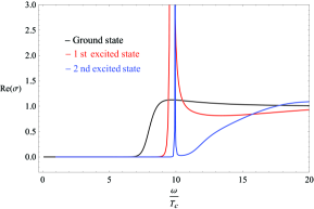
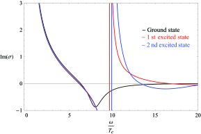
Figure 3: The real and imaginary parts of optical conductivity as a function of the frequency. In both plots, the black, red and blue lines denote ground state, first and second states, respectively.

In Fig. 3, we plot the conductivity as a function of the frequency at the low temperature $T/T_{c}\simeq 0.1$ for the operators ${\mathcal{O}}_{2}$ of excited states. The left and right panels correspond to the real and imaginary parts of conductivity, respectively. In both plots, the black, red and blue lines denote the ground state, first and second states, respectively. Similar to the ground state, there also exists a gap in the conductivity of the excited state. It is interesting to note that for the excited states, there exists an additional pole in $\text{Im}[\sigma]$ and a delta function in $\text{Re}[\sigma]$ arising at low temperature inside the gap. In addition, the form of delta function of each higher excited states in $\text{Re}[\sigma]$ has the narrower width. In [44], there exists the similar configurations of the conductivity as $m^{2}=-9/4$, and the authors pointed out that since holographic superconductors are strongly coupled, there exist the interactions between the quasiparticles excited above the superconducting ground state, and the pole indicates that the interactions could be very strong and form a bound state. Now, it is clear that these behaviors are just the evidence of the existence of the excited states of holographic superconductor. Similar behaviours for conductivities were also found in the type II Goldstone bosons [46]. The authors related this behaviour of conductivities to the fact that these are not in the true ground state of the theory, and complemented the discussion by computing the quasinormal mode and confirm this picture. Furthermore, in [47] they computed the correct ground state. So, these above behaviors of conductivities indicate the emergence of new bound states, which embodies the existence of excited states.

4 Discussion

In this paper, we reconsidered the static solutions of Einstein gravity coupled with Maxwell and a free, massive scalar field in four-dimensional AdS spacetime. Besides the well-known ground state solution of holographic superconductor, we constructed the numerical solutions of holographic supercondecutor with excited states, including the case of operators ${\mathcal{O}}_{1}$ and ${\mathcal{O}}_{2}$. Comparing with the ground state solution in [5], we found that when the temperature drops below the critical temperature $T_{c}^{(0)}$, the condensate of holographic superconductor begin to appear, which could be regarded as the ground state solution. Further decreasing the temperature to $T_{c}^{(1)}$, a new branch of solution with a node in radial direction begins to develop, which is the first excited state solution. As the temperature continues to decrease to lower values, we could obtain a series of excited states of holographic superconductor with differential critical temperatures. It is well-known that the condensate of ground state for the operator $\langle\mathcal{O}_{1}\rangle$ appears to diverge as the temperature $T\rightarrow 0$. However, the condensate of excited states does not appear to diverge and goes to a constant near zero temperature. Moreover, the condensate of the excited state is smaller than the ground state. Note that the value of the condensate for the second excited state near zero temperature is very closed to that of the first excited state. We calculated the condensate $\langle\mathcal{O}_{1}\rangle$ near zero temperature until the sixth excited state, and found that this value is about 4.4. For the operator $\mathcal{O}_{2}$, the condensate of an excited state is larger than the ground state. We also studied the conductivity in the excited states of holographic superconductors. It is very interesting to mention that each excited state has an additional pole in $\text{Im}[\sigma]$ and a delta function in $\text{Re}[\sigma]$ arising at the low temperature inside the gap. These behaviors are just the evidence of the existence of the excited states.

Since in this paper we are using AdS/CFT to describe the superconductor with excite states, it is natural to ask what is the connection between holographic superconductor with excite states and actual superconductor matter in condensed physics. It is well known that if a thermodynamic system is in equilibrium state, it should be in the state with the minimum free energy. Holographic model of superconductor investigated in [35, 36] could correspond to the above state of minimum free energy. But for mesoscopic systems, such as nanostructures, due to the small size of the system and the small number of particles. The fluctuation of the system may make it run to a metastable state. Thus, these free energy surfaces are very complex and have many metastable states. The system can stay on these states for a long time. In case of superconductors, it means that the sample should have one size at least of order the coherence length, and such superconductors are called mesoscopic superconductors [48]. In [49], with the time-dependent Ginzburg-Landau equations, transitions between metastable states of a superconducting ring are investigated. So, excited states of holographic superconductor could be related to the metastable states of mesoscopic superconductors.

There are many interesting extensions of our work. First, we have noticed that the value of the condensate $\langle\mathcal{O}_{1}\rangle$ near zero temperature with higher excited state is about 4.4. In addition, the difference of the critical chemical potential $\mu_{c}$ between the consecutive states is about $5$ for both of the condensates $\langle\mathcal{O}_{1}\rangle$ and $\langle\mathcal{O}_{2}\rangle$, but the reason of these configurations is not clear. It would be very interesting to study these cases with the semi-analytical method [45] to see how these values are related to excited states. The second extension of our study is that away from the large charge limit, the backreaction of the matter fields on the bulk metric needs to be included. Thus, one must solve the coupled differential equations including Einstein equations. Finally, we are planning to study the excited states of the p-wave and d-wave holographic superconductor and construct the excited vector and tensor condensates in the background of black hole in future work.

Acknowledgements

We would like to thank Ying Zhong and Cheng-Long Jia for helpful discussion. Parts of computations were performed on the shared memory system at institute of computational physics and complex systems in Lanzhou university. This work was supported by the National Natural Science Foundation of China (Grants No. 11875151 and No. 11522541).

References

- [1] J. M. Maldacena, “The Large N limit of superconformal field theories and supergravity,” Int. J. Theor. Phys. 38, 1113 (1999) [Adv. Theor. Math. Phys. 2, 231 (1998)] doi:10.1023/A:1026654312961, 10.4310/ATMP.1998.v2.n2.a1 [hep-th/9711200].
- [2] E. Witten, “Anti-de Sitter space and holography,” Adv. Theor. Math. Phys. 2, 253 (1998) doi:10.4310/ATMP.1998.v2.n2.a2 [hep-th/9802150].
- [3] O. Aharony, S. S. Gubser, J. M. Maldacena, H. Ooguri and Y. Oz, “Large N field theories, string theory and gravity,” Phys. Rept. 323, 183 (2000) doi:10.1016/S0370-1573(99)00083-6 [hep-th/9905111].
- [4] S. S. Gubser, “Breaking an Abelian gauge symmetry near a black hole horizon,” Phys. Rev. D 78, 065034 (2008) [arXiv:0801.2977 [hep-th]].
- [5] S. A. Hartnoll, C. P. Herzog and G. T. Horowitz, “Building a holographic superconductor,” Phys. Rev. Lett. 101, 031601 (2008) [arXiv:0803.3295 [hep-th]].
- [6] S. A. Hartnoll, C. P. Herzog and G. T. Horowitz, “Holographic superconductors,” JHEP 0812, 015 (2008) [arXiv:0810.1563 [hep-th]].
- [7] J. W. Chen, Y. J. Kao, D. Maity, W. Y. Wen and C. P. Yeh, “Towards A Holographic Model of D-Wave Superconductors,” Phys. Rev. D 81, 106008 (2010) [arXiv:1003.2991 [hep-th]].
- [8] F. Benini, C. P. Herzog, R. Rahman and A. Yarom, “Gauge gravity duality for d-wave superconductors: prospects and challenges,” JHEP 1011, 137 (2010) [arXiv:1007.1981 [hep-th]].
- [9] K. -Y. Kim and M. Taylor, “Holographic d-wave superconductors,” JHEP 1308, 112 (2013) [arXiv:1304.6729 [hep-th]].
- [10] S. S. Gubser and S. S. Pufu, “The Gravity dual of a p-wave superconductor,” JHEP 0811, 033 (2008) [arXiv:0805.2960 [hep-th]].
- [11] F. Aprile, D. Rodriguez-Gomez and J. G. Russo, “p-wave Holographic Superconductors and five-dimensional gauged Supergravity,” JHEP 1101, 056 (2011) doi:10.1007/JHEP01(2011)056 [arXiv:1011.2172 [hep-th]].
- [12] R. G. Cai, S. He, L. Li and L. F. Li, “A Holographic Study on Vector Condensate Induced by a Magnetic Field,” JHEP 1312, 036 (2013) doi:10.1007/JHEP12(2013)036 [arXiv:1309.2098 [hep-th]].
- [13] R. G. Cai, L. Li and L. F. Li, “A Holographic P-wave Superconductor Model,” JHEP 1401, 032 (2014) doi:10.1007/JHEP01(2014)032 [arXiv:1309.4877 [hep-th]].
- [14] G. T. Horowitz, J. E. Santos and B. Way, “A holographic Josephson junction,” Phys. Rev. Lett. 106, 221601 (2011) [arXiv:1101.3326 [hep-th]].
- [15] Y. Q. Wang, Y. X. Liu and Z. H. Zhao, “Holographic Josephson junction in 3+1 dimensions,” [arXiv:1104.4303 [hep-th]].
- [16] M. Siani, “On inhomogeneous holographic superconductors,” [arXiv:1104.4463 [hep-th]].
- [17] E. Kiritsis and V. Niarchos, “Josephson junctions and AdS/CFT networks,” JHEP 1107, 112 (2011) [Erratum-ibid. 1110, 095 (2011)] [arXiv:1105.6100 [hep-th]].
- [18] Y. Q. Wang, Y. X. Liu and Z. H. Zhao, “Holographic p-wave Josephson junction,” [arXiv:1109.4426 [hep-th]].
- [19] Y. Q. Wang, Y. X. Liu, R. G. Cai, S. Takeuchi and H. Q. Zhang, “Holographic SIS Josephson junction,” JHEP 1209, 058 (2012) [arXiv:1205.4406 [hep-th]].
- [20] R. G. Cai, Y. Q. Wang and H. Q. Zhang, “A holographic model of SQUID,” JHEP 1401, 039 (2014) [arXiv:1308.5088 [hep-th]].
- [21] S. Takeuchi, “Holographic Superconducting Quantum Interference Device,” Int. J. Mod. Phys. A 30, no. 09, 1550040 (2015) [arXiv:1309.5641 [hep-th]].
- [22] H. F. Li, L. Li, Y. Q. Wang and H. Q. Zhang, “Non-relativistic Josephson Junction from Holography,” JHEP 1412, 099 (2014) [arXiv:1410.5578 [hep-th]].
- [23] S. Liu and Y. Q. Wang, “Holographic model of hybrid and coexisting s-wave and p-wave Josephson junction,” Eur. Phys. J. C 75, no. 10, 493 (2015) doi:10.1140/epjc/s10052-015-3692-2 [arXiv:1504.06918 [hep-th]].
- [24] Y. P. Hu, H. F. Li, H. B. Zeng and H. Q. Zhang, “Holographic Josephson Junction from Massive Gravity,” Phys. Rev. D 93, no. 10, 104009 (2016) doi:10.1103/PhysRevD.93.104009 [arXiv:1512.07035 [hep-th]].
- [25] Y. Q. Wang and S. Liu, “Holographic s-wave and p-wave Josephson junction with backreaction,” JHEP 1611, 127 (2016) doi:10.1007/JHEP11(2016)127 [arXiv:1608.06364 [hep-th]].
- [26] B. Kiczek, M. Rogatko and K. I. Wysokinski, “DC SQUID as a sensitive detector of dark matter,” arXiv:1904.00653 [hep-th].
- [27] B. D. Josephson, “Possible new effects in superconductive tunnelling,” Phys. Lett. 1, 251 (1962).
- [28] S. S. Gubser, C. P. Herzog, S. S. Pufu and T. Tesileanu, “Superconductors from Superstrings,” Phys. Rev. Lett. 103, 141601 (2009) doi:10.1103/PhysRevLett.103.141601 [arXiv:0907.3510 [hep-th]].
- [29] J. P. Gauntlett, J. Sonner and T. Wiseman, “Holographic superconductivity in M-Theory,” Phys. Rev. Lett. 103, 151601 (2009) doi:10.1103/PhysRevLett.103.151601 [arXiv:0907.3796 [hep-th]].
- [30] J. P. Gauntlett, J. Sonner and T. Wiseman, “Quantum Criticality and Holographic Superconductors in M-theory,” JHEP 1002, 060 (2010) doi:10.1007/JHEP02(2010)060 [arXiv:0912.0512 [hep-th]].
- [31] S. A. Hartnoll, “Lectures on holographic methods for condensed matter physics,” Class. Quant. Grav. 26, 224002 (2009) [arXiv:0903.3246 [hep-th]].
- [32] C. P. Herzog, “Lectures on holographic superfluidity and superconductivity,” J. Phys. A 42, 343001 (2009) [arXiv:0904.1975 [hep-th]].
- [33] G. T. Horowitz, “Introduction to holographic superconductors,” Lect. Notes Phys. 828, 313 (2011) [arXiv:1002.1722 [hep-th]].
- [34] R. G. Cai, L. Li, L. F. Li and R. Q. Yang, “Introduction to Holographic Superconductor Models,” Sci. China Phys. Mech. Astron. 58, no. 6, 060401 (2015) [arXiv:1502.00437 [hep-th]].
- [35] S. S. Gubser and A. Nellore, “Ground states of holographic superconductors,” Phys. Rev. D 80, 105007 (2009) doi:10.1103/PhysRevD.80.105007 [arXiv:0908.1972 [hep-th]].
- [36] G. T. Horowitz and M. M. Roberts, “Zero Temperature Limit of Holographic Superconductors,” JHEP 0911, 015 (2009) doi:10.1088/1126-6708/2009/11/015 [arXiv:0908.3677 [hep-th]].
- [37] J. Erlich, E. Katz, D. T. Son and M. A. Stephanov, “QCD and a holographic model of hadrons,” Phys. Rev. Lett. 95, 261602 (2005) doi:10.1103/PhysRevLett.95.261602 [hep-ph/0501128].
- [38] A. Karch, E. Katz, D. T. Son and M. A. Stephanov, “Linear confinement and AdS/QCD,” Phys. Rev. D 74, 015005 (2006) doi:10.1103/PhysRevD.74.015005 [hep-ph/0602229].
- [39] K. Ghoroku and M. Yahiro, “Holographic model for mesons at finite temperature,” Phys. Rev. D 73, 125010 (2006) doi:10.1103/PhysRevD.73.125010 [hep-ph/0512289].
- [40] S. S. Afonin, “AdS/QCD models describing a finite number of excited mesons with Regge spectrum,” Phys. Lett. B 675, 54 (2009) doi:10.1016/j.physletb.2009.03.073 [arXiv:0903.0322 [hep-ph]].
- [41] M. Fujita, K. Fukushima, T. Misumi and M. Murata, “Finite-temperature spectral function of the vector mesons in an AdS/QCD model,” Phys. Rev. D 80, 035001 (2009) doi:10.1103/PhysRevD.80.035001 [arXiv:0903.2316 [hep-ph]].
- [42] L. X. Cui, S. Takeuchi and Y. L. Wu, “Thermal Mass Spectra of Vector and Axial-Vector Mesons in Predictive Soft-Wall AdS/QCD Model,” JHEP 04, 144 (2012) doi:10.1007/JHEP04(2012)144 [arXiv:1112.5923 [hep-ph]].
- [43] P. Breitenlohner and D. Z. Freedman, “Positive energy in anti-De Sitter backgrounds and gauged extended supergravity,” Phys. Lett. B 115, 197 (1982).
- [44] G. T. Horowitz and M. M. Roberts, “Holographic Superconductors with Various Condensates,” Phys. Rev. D 78, 126008 (2008) doi:10.1103/PhysRevD.78.126008 [arXiv:0810.1077 [hep-th]].
- [45] G. Siopsis and J. Therrien, “Analytic Calculation of Properties of Holographic Superconductors,” JHEP 1005, 013 (2010) doi:10.1007/JHEP05(2010)013 [arXiv:1003.4275 [hep-th]].
- [46] I. Amado, D. Arean, A. Jimenez-Alba, K. Landsteiner, L. Melgar and I. S. Landea, “Holographic Type II Goldstone bosons,” JHEP 1307, 108 (2013) doi:10.1007/JHEP07(2013)108 [arXiv:1302.5641 [hep-th]].
- [47] I. Amado, D. Arean, A. Jimenez-Alba, L. Melgar and I. Salazar Landea, “Holographic s+p Superconductors,” Phys. Rev. D 89, no. 2, 026009 (2014) doi:10.1103/PhysRevD.89.026009 [arXiv:1309.5086 [hep-th]].
- [48] F. Peeters, V. Schweigert, B. Baelus and P. Deo, “Vortex Matter in Mesoscopic Superconducting Disks and Rings,” Physica C 332, 255 (2000).
- [49] D.Y. Vodolazov, F.M. Peeters “Dynamic transitions between metastable states in a superconducting ring,” Phys. Rev. B 66, 054537 (2002)