Computing Essential Sets for Convex and Non-convex Scenario Problems: Theory and Application

Abstract

The scenario approach is a general data-driven algorithm to chance-constrained optimization. It seeks the optimal solution that is feasible to a carefully chosen number of scenarios. A crucial step in the scenario approach is to compute the cardinality of essential sets, which is the smallest subset of scenarios that determine the optimal solution. This paper addresses the challenge of efficiently identifying essential sets. For convex problems, we demonstrate that the sparsest dual solution of the scenario problem could pinpoint the essential set. For non-convex problems, we show that two simple algorithms return the essential set when the scenario problem is non-degenerate. Finally, we illustrate the theoretical results and computational algorithms on security-constrained unit commitment (SCUC) in power systems. In particular, case studies of chance-constrained SCUC are performed in the IEEE 118-bus system. Numerical results suggest that the scenario approach could be an attractive solution to practical power system applications.

Chance constraint, scenario approach, convex optimization, non-convex, unit commitment.

1 Introduction

Decision making in the presence of uncertainties is an important problem in both theory and practice. Stochastic optimization (SO) and robust optimization (RO) are two common approaches for decision making under uncertainties. SO relies on probabilistic models to depict uncertainties and often optimizes the objective function in the presence of randomness [1]. RO takes an alternative approach, in which the uncertainty model is typically set-based and deterministic [2]. This paper provides a perspective of decision making in uncertain environments through the lens of chance-constrained optimization (CCO), which is akin to both SO and RO [3]. The main distinction between CCO and SO/RO is the chance constraint (see (1b) and (2b) in Section 2), which explicitly considers the feasibility of solutions under uncertainties.

CCO has found successful applications in many different areas, e.g., control theory [4], chemical process [5] and power systems [6]. Since the first chance-constrained program was formulated in 1950s [7], many classical methods were proposed to deal with specific families of distributions, e.g., multivariate Gaussian distribution [8], log-concave distributions [9]. Some breakthroughs and novel methods appeared in the past ten years, including (1) sample average approximation (SAA) [10, 11, 12, 13, 14, 15, 16, 17]; (2) safe approximation [18, 19, 20, 21, 22, 23]; and (3) the scenario approach [24, 25, 26, 27, 28, 29]. Some key results and recent progresses are summarized below, a more comprehensive review is in [3].

SAA is closely related with stochastic programming. [10] first introduced the idea of approximating the violation probability using samples. Based on this idea, [11, 12, 13] show that CCO problems can be approximated by mixed integer programs (MIPs). Many recent results have been developed on the computational and theoretical aspects of SAA. [13] proposes different strong MIP formulations for SAA, and various techniques to accelerate solving SAA have been proposed, e.g, [13, 15]. Reference [16] studies the case of finite distributions and discusses existing approximation approaches for constructing good feasible solution. [17] proposes new Lagrangian dual based formulations that are proved to be superior than standard MIP formulations.

An alternative approach to CCO is safe approximation (or inner approximation), whose solutions are guaranteed to satisfy the chance constraint. The safe approximation is often convex problems that are tractable to solve, e.g., [18, 21, 19, 20]. This line of work is closely related with robust optimization. For example, the safe approximations in [19, 20, 21, 22] can be written as RO problems using uncertainty sets. Reference [23] further shows that RO problems with carefully constructed uncertainty sets could return optimal solutions that satisfy chance constraints with high confidence. [30] derives a conic formulation to approximate a CCO problem with linear constraints, and applies a cutting plane algorithm to solve it. Another related work is [31], which develops outer approximations to CCO problems and obtain lower bounds on the optimal objective value.

The scenario approach (also known as scenario approximation) is another popular approach to solve CCO problems. The scenario approach seeks the optimal solution that is feasible to a carefully chosen number of scenarios (sample complexity). Reference [24] first proved a lower bound on sample complexity. Later [25, 26, 27] significantly improved the sample complexity bound and show that the bound is tight for a special class of CCO problems. The classical scenario approach in [24, 25, 26, 27] require all constraints to be convex, thus not applicable to non-convex problems. A recent breakthrough[29] extends the scenario approach theory towards non-convex problems. For both convex and non-convex scenario approach, there is a critical step in common: estimating or computing the cardinality of essential sets, which is defined as the smallest subset of scenarios that determine the optimal solution (see Definitions 2 and 6).

This paper addresses the challenge of efficiently identifying the cardinality of essential sets for both convex and non-convex scenario problems. The main contributions of this paper are threefold.

From the theoretical perspective, we connect the convex scenario approach theory with recent progress under the non-convex setting, we reveal the connection and distinction among similar concepts defined in different contexts, i.e., support scenarios [25] and essential sets [27] in the convex setting, irreducible and minimum support subsample [29] in the non-convex setting. We also extend the classical results on the structure of convex scenario problems in [27] towards non-convex problems.

From the algorithmic perspective, we design algorithms that can efficiently identify essential sets. For convex problems, essential sets can be pinpointed using the sparsest dual solution (Theorem 5). For non-convex problems, we show that simple algorithms based on definitions return the essential set when the scenario problem is non-degenerate (Theorem 4).

From the application perspective, we provide a practical solution of chance-constrained Security-constrained Unit Commitment (c-SCUC) using the scenario approach. To the best of our knowledge, this paper is the first to apply the scenario approach on c-SCUC while providing theoretical guarantees on the feasibility of solution. Based on the special two-stage structure of scenario-based SCUC (s-SCUC), it is possible to design efficient algorithms to identify essential sets despite of the non-convexity of s-SCUC.

The remainder of this paper is organized as follows. Section 2 introduces the scenario approach for both convex and non-convex problems. Section 3 studies the properties of essential sets in convex and non-convex scenario problems and proposes various algorithms to identify essential sets. Section 4 formulates chance-constrained SCUC, which is solved via the scenario approach. Numerical results and discussions are in Section 5 and 6, respectively. Section 7 presents the concluding remarks. All proofs are available at [36].

The notations in this paper are standard. All vectors are in the real field $\mathbf{R}$. We use $\mathbf{1}$ to represent an all-one vector of appropriate size. The transpose of a vector $a$ is $a^{\intercal}$. The element-wise multiplication of the same-size vectors $a$ and $b$ is denoted by $a\circ b$. For instance, $[a_{1};a_{2}]\circ[b_{1};b_{2}]=[a_{1}b_{1};a_{2}b_{2}]$. Sets are in calligraphy fonts, e.g., $\mathcal{S}$. The cardinality of a set $\mathcal{S}$ is $|\mathcal{S}|$. Removal of element $i$ from set $\mathcal{N}$ is represented by $\mathcal{N}-i$. The essential supremum is $\operatorname*{ess\,sup}$.

2 Introduction to the Scenario Approach

2.1 Chance-constrained Optimization (CCO)

The typical formulation of CCO is in (1).

$$\min_{x}~{} c^{\intercal}x$$ (1a)

s.t. $$\mathbb{P}_{\xi}\Big{(}f(x,\xi)\leq 0\Big{)}\geq 1-\epsilon$$ (1b)

$$g(x)\leq 0$$ (1c)

We could write (1) in a more compact form by defining $\mathcal{X}_{\xi}:=\{x\in\mathbf{R}^{n}:f(x,\xi)\leq 0\}$ and $\chi:=\{x\in\mathbf{R}^{n}:g(x)\leq 0\}$

$$\min_{x\in\chi}~{} c^{\intercal}x$$ (2a)

s.t. $$\mathbb{P}_{\xi}\Big{(}x\in\mathcal{X}_{\xi}\Big{)}\geq 1-\epsilon$$ (2b)

Without loss of generality, we assume that the objective is a linear function of decision variables $x\in\mathbf{R}^{d}$ [26]. Random vector $\xi\in\Xi$ denotes the source of uncertainties and $\Xi$ is the support of $\xi$. Deterministic constraints (1c) are represented by set $\chi$ in (2). Constraint (1b) or (2b) is the chance constraint. The chance constraint (2b) requires the the inner constraint $x\in\mathcal{X}_{\xi}$ to be satisfied with probability at least $1-\epsilon$, where the violation probability $\epsilon$ is typically a small number (e.g., $1\%,5\%$). In (2b), the set $\mathcal{X}_{\xi}$ depends on the realization of $\xi$ and the probability is taken with respect to $\xi$.

As discussed in Section 1, many methods have been proposed to solve chance-constrained optimization problems. A detailed review and tutorial on chance-constrained optimization is in [3]. Compared with other methods, the scenario approach has many advantages such as computationally efficient and applicable for a broad range of optimization problems.

2.2 The Scenario Approach for Convex Problems

The scenario approach utilizes $N$ independent and identically distributed (i.i.d.) scenarios $\mathcal{N}:=\{\xi^{1},\xi^{2},\cdots,\xi^{N}\}$ to approximate the chance-constrained program (1) with the scenario problem below:

$$\text{SP}(\mathcal{N}):~{}\min_{x}\quad c^{\intercal}x$$ (3a)

s.t. $$f(x,\xi^{1})\leq 0 :\mu^{1}$$ (3b)

$$\qquad\vdots$$

$$f(x,\xi^{N})\leq 0 :\mu^{N}$$ (3c)

$$g(x)\leq 0 :\lambda$$ (3d)

The scenario problem $\operatorname{\text{SP}}(\operatorname{\mathcal{N}})$ seeks the optimal solution $x_{\mathcal{N}}^{*}$ that is feasible for all $N$ scenarios. The Lagrangian multiplier associated with the $i$th scenario constraint $f(x,\xi^{i})\leq 0$ is denoted by $\mu^{i}\in\mathbf{R}^{m}$. We can write the scenario problem $\operatorname{\text{SP}}(\operatorname{\mathcal{N}})$ in a similar way with (2) by defining $\mathcal{X}_{i}:=\{x\in\mathbf{R}^{n}:f(x,\xi^{i})\leq 0\}$.

$$\text{SP}(\mathcal{N}):~{}\min_{x\in\chi}~{} c^{\intercal}x$$ (4a)

s.t. $$x\in\cap_{i=1}^{N}\mathcal{X}_{i}$$ (4b)

Definition 1 (Violation Probability).

The violation probability of a candidate solution $x^{\diamond}$ is defined as the probability that $x^{\diamond}$ is infeasible:

$$\mathbb{V}(x^{\diamond}):=\mathbb{P}_{\xi}\big{(}x^{\diamond}\notin\mathcal{X}_{\xi}\big{)}.$$ (5)

The scenario approach theory aims at answering the following sample complexity question: what is the smallest sample size $N$ such that $x_{\mathcal{N}}^{*}$ is feasible (i.e., $\mathbb{V}(x_{\mathcal{N}}^{*})\leq\epsilon$) to the original chance-constrained program (2)? Reference [25, 27] provide in-depth analysis based on the concept of support scenarios.

Definition 2 (Support Scenario [25, 27]).

Scenario $\xi^{i}$ is a support scenario for the scenario problem $\operatorname{\text{SP}}(\operatorname{\mathcal{N}})$ if its removal changes the solution of $\operatorname{\text{SP}}(\operatorname{\mathcal{N}})$.

Let $x_{\operatorname{\mathcal{N}}}^{*}$ and $x_{\operatorname{\mathcal{N}}-i}^{*}$ stand for the optimal solution to scenario problems $\operatorname{\text{SP}}(\operatorname{\mathcal{N}})$ and $\operatorname{\text{SP}}(\operatorname{\mathcal{N}}-i)$, respectively. Then scenario $\xi^{i}$ is a support scenario if $c^{\intercal}x_{\operatorname{\mathcal{N}}-i}^{*}<c^{\intercal}x_{\operatorname{\mathcal{N}}}^{*}$. We use $\operatorname{\mathcal{S}}(\operatorname{\mathcal{N}})$ ($\operatorname{\mathcal{S}}$ in short) to represent the set of all support scenarios of $\operatorname{\text{SP}}(\operatorname{\mathcal{N}})$.

Definition 3 (Non-degenerate Scenario Problem [25, 27]).

Let $x_{\mathcal{N}}^{*}$ and $x_{\mathcal{S}}^{*}$ be the optimal solutions to the scenario problems $\operatorname{\text{SP}}(\operatorname{\mathcal{N}})$ and $\operatorname{\text{SP}}(\operatorname{\mathcal{S}})$, respectively. The scenario problem $\operatorname{\text{SP}}(\operatorname{\mathcal{N}})$ is said to be non-degenerate, if $c^{\intercal}x_{\mathcal{N}}^{*}=c^{\intercal}x_{\mathcal{S}}^{*}$.

Assumption 1 (Non-degeneracy[25, 27]).

For every $N$, the scenario problem $\operatorname{\text{SP}}(\operatorname{\mathcal{N}})$ is non-degenerate with probability $1$ with respect to scenarios $\operatorname{\mathcal{N}}=\{\xi^{1},\xi^{2},\cdots,\xi^{N}\}$.

Assumption 2 (Feasibility [25]).

Every scenario problem $\operatorname{\text{SP}}(\operatorname{\mathcal{N}})$ is feasible, and its feasibility region has a non-empty interior. The optimal solution $x_{\mathcal{N}}^{\ast}$ of $\operatorname{\text{SP}}(\operatorname{\mathcal{N}})$ exists.

Definition 4 (Helly’s Dimension [27]).

Helly’s dimension of the scenario problem $\operatorname{\text{SP}}(\operatorname{\mathcal{N}})$ is the smallest integer $h$ that $h\geq\operatorname*{ess\,sup}_{\operatorname{\mathcal{N}}\subseteq\Xi^{N}}|\operatorname{\mathcal{S}}(\operatorname{\mathcal{N}})|$ holds for any finite $N\geq 1$, where $|\operatorname{\mathcal{S}}(\operatorname{\mathcal{N}})|$ is the number of support scenarios.

Theorem 1 presents one of the most important results in the scenario approach theory, which is based on the non-degeneracy and feasibility assumptions.

Theorem 1 (Exact Feasibility [25, 27]).

Under Assumptions 1 (non-degeneracy) and 2 (feasibility), let $x_{\operatorname{\mathcal{N}}}^{\ast}$ be the optimal solution to the scenario problem $\operatorname{\text{SP}}(\operatorname{\mathcal{N}})$, it holds that

$$\mathbb{P}^{N}\Big{(}\mathbb{V}(x_{\operatorname{\mathcal{N}}}^{\ast})>\epsilon\Big{)}\leq\sum_{i=1}^{h-1}\binom{N}{i}\epsilon^{i}(1-\epsilon)^{N-i}.$$ (6)

The probability $\mathbb{P}^{N}$ is taken with respect to $N$ random scenarios $\mathcal{N}=\{\xi^{i}\}_{i=1}^{N}$, and $h$ is the Helly’s dimension of $\operatorname{\text{SP}}(\operatorname{\mathcal{N}})$.

Stronger results without the feasibility assumption are in [27, 25]. Based on Theorem 1, the scenario approach answers the sample complexity question in Corollary 1.

Corollary 1 (Sample Complexity [25, 27]).

Under Assumptions 1 (non-degeneracy) and 2 (feasibility), given a violation probability $\epsilon\in(0,1)$ and a confidence parameter $\beta\in(0,1)$, if we choose the smallest number of scenarios $N$ such that

$$\sum_{i=0}^{h-1}\binom{N}{i}\epsilon^{i}(1-\epsilon)^{N-i}\leq\beta,$$ (7)

then it holds that

$$\mathbb{P}^{N}\Big{(}\mathbb{V}(x_{\mathcal{N}}^{\ast})\leq\epsilon\Big{)}\geq 1-\beta,$$ (8)

where $x_{\mathcal{N}}^{\ast}$ is the optimal solution to $\operatorname{\text{SP}}(\operatorname{\mathcal{N}})$, and $h$ is the Helly’s dimension of $\operatorname{\text{SP}}(\operatorname{\mathcal{N}})$ ($0\leq h\leq N$).

The scenario approach is essentially a randomized algorithm to find a feasible solution to chance-constrained optimization problems. The randomness of the scenario approach comes from drawing i.i.d. scenarios. The confidence parameter $\beta$ quantifies the risk of failure due to drawing scenarios from a “bad” set. Corollary 1 shows that by choosing a proper number of scenarios, the corresponding optimal solution $x_{\mathcal{N}}^{*}$ is feasible (i.e., $\mathbb{V}(x_{\operatorname{\mathcal{N}}}^{*})\leq\epsilon$) with confidence at least $1-\beta$.

Assumption 3 (Convexity).

The deterministic constraint $g(x)\leq 0$ is convex, and the random constraint $f(x,\xi)$ is convex in $x$ for every instance of $\xi$. In other words, the sets $\chi$ and $\mathcal{X}_{i}$s in (4) are convex.

Theorem 2 ([24, 27]).

Under Assumption 2 and 3, the number of support scenarios $|\operatorname{\mathcal{S}}|$ for $\operatorname{\text{SP}}(\operatorname{\mathcal{N}})$ is at most $n$. In other words, $h\leq n$, where $n$ is the number of decision variables $x\in\mathbf{R}^{n}$ and $h$ is Helly’s dimension.

For convex scenario problems $\operatorname{\text{SP}}(\operatorname{\mathcal{N}})$, we could replace $h$ by $n$ in Theorem 1 and Corollary 1. This leads to the classical results of the scenario approach in [24, 25, 26, 27].

Remark 1 (Towards Non-convexity).

Theorem 1 and Corollary 1 do not assume convexity of $f(x,\xi)$ and $g(x)$. In theory, Theorem 1 and Corollary 1 are applicable for non-convex scenario problems if a feasible non-convex $\operatorname{\text{SP}}(\operatorname{\mathcal{N}})$ is proved to be non-degenerate with probability $1$ (e.g., [32]). In practice, however, the scenario approach was considered not applicable for non-convex problems. Comprehensive analysis are presented in Section 2.3.

2.3 The Scenario Approach for Non-convex Problems

The scenario approach was considered not applicable for non-convex problems for the following three reasons: (1) non-convexity causes degeneracy; (2) non-trivial bounds on $|\operatorname{\mathcal{S}}|$ may not exist for non-convex $\operatorname{\text{SP}}(\operatorname{\mathcal{N}})$; and (3) it is computationally intractable to find optimal solutions.

First, degeneracy is a common issue for non-convex problems, e.g., the scenario-based SCUC problem in Section 4.5. Since the non-degeneracy assumption 1 lies at the heart of the scenario approach theory, almost all results in the literature are for non-degenerate problems.

Second, it is almost impossible to prove non-trivial and practical bounds on the number of support scenarios $|\operatorname{\mathcal{S}}|$ for non-convex problems. Reference [29] presents one extreme case, in which every scenario is a support scenario thus $|\operatorname{\mathcal{S}}|=N$ . In addition, a loose bound typically leads to an astronomical sample complexity $N$, which make the scenario approach unpractical. For instance, loose bounds on $|\operatorname{\mathcal{S}}|$ for scenario-based unit commitment will require $10^{3}\sim 10^{4}$ times more scenarios than necessary [32].

Furthermore, the most attractive feature of convex optimization is that any local minimum is a global minimum. And there exist a broad family of efficient algorithms that compute global optimal solutions for convex problems. Hence, $x_{\operatorname{\mathcal{N}}}^{*}$ in Section 2.2 refers to the global optimal solution by default. It is worth noting that $x_{\operatorname{\mathcal{N}}}^{*}$ is solely determined by the scenario problem $\operatorname{\text{SP}}(\operatorname{\mathcal{N}})$ and it is not algorithm-dependent.

For non-convex problems, however, it is often computationally intractable to find global optimal solutions. There are many algorithms that are capable of finding local optimal solutions in a relatively short time. Therefore, it is more reasonable and practical to analyze the characteristics of local solutions for non-convex scenario problems. Algorithm $\mathbb{A}:\Xi^{N}\rightarrow\mathbf{R}^{n}$ stands for the process of finding solutions to $\operatorname{\text{SP}}(\operatorname{\mathcal{N}})$, e.g., primal-dual interior-point method. We use $\operatorname{\text{opx}}_{\mathbb{A}}(\operatorname{\mathcal{N}})$ to represent a (possibly suboptimal) solution to $\operatorname{\text{SP}}(\operatorname{\mathcal{N}})$ obtained via algorithm $\mathbb{A}$. The corresponding optimal objective value is denoted by $\operatorname{\text{opt}}_{\mathbb{A}}(\operatorname{\mathcal{N}})$. The subscript $\mathbb{A}$ emphasizes the fact that the solution is algorithm-dependent. And we use $\operatorname{\text{SP}}_{\mathbb{A}}(\operatorname{\mathcal{N}})$ to represent a scenario problem solved by algorithm $\mathbb{A}$.

Consequently, the scenario approach was considered not applicable for non-convex problems until very recently. By removing the non-degeneracy assumption and analyzing any feasible solutions of non-convex scenario problems, reference [29] develops a general theory for the scenario approach. This subsection summarizes its key results.

Identical to the convex case in Section 2.2, the scenario approach approximates (2) to the scenario problem (4) using $N$ scenarios $\mathcal{N}=\{\xi^{1},\xi^{2},\cdots,\xi^{N}\}$ for non-convex problems. The sets $\chi$ and $\mathcal{X}_{\xi}$ here could be non-convex.

Definition 5 (Invariant Set).

Let $\operatorname{\text{opt}}_{\mathbb{A}}(\mathcal{M})$ be the optimal value of $\operatorname{\text{SP}}(\mathcal{M})$ found by algorithm $\mathbb{A}$ for a scenario problem $\operatorname{\text{SP}}(\mathcal{M})$. A set of scenarios $\mathcal{I}$ is an invariant (scenario) set for $\operatorname{\text{SP}}_{\mathbb{A}}(\operatorname{\mathcal{N}})$ if $\operatorname{\text{opt}}_{\mathbb{A}}(\mathcal{I})=\operatorname{\text{opt}}_{\mathbb{A}}(\operatorname{\mathcal{N}})$.

The concept of invariant set is an extension of support scenarios for (possibly degenerate) non-convex scenario problems. A trivial invariant set is $\operatorname{\mathcal{I}}=\operatorname{\mathcal{N}}$. Algorithm $\mathbb{B}:\Xi^{N}\rightarrow\operatorname{\mathcal{I}}$ represents the process of finding non-trivial invariant sets. Examples of Algorithm $\mathbb{B}$ can be found in Section 3 and Appendix 9.

Theorem 3 (Posterior Guarantees for Non-convex Scenario Problems [29]).

Suppose Assumption 2 (feasibility) holds true and $\beta\in(0,1)$ is given. Algorithm $\mathbb{A}$ solves the scenario problem $\operatorname{\text{SP}}(\operatorname{\mathcal{N}})$ and obtains an optimal solution $\operatorname{\text{opx}}_{\mathbb{A}}(\operatorname{\mathcal{N}})$. Algorithm $\mathbb{B}$ finds an invariant set $\mathcal{I}$ of cardinality $|\operatorname{\mathcal{I}}|$. The following probabilistic guarantee holds

$$\mathbb{P}^{N}\Big{(}\mathbb{V}\big{(}\operatorname{\text{opx}}_{\mathbb{A}}(\operatorname{\mathcal{N}})\big{)}\leq\epsilon(N,|\operatorname{\mathcal{I}}|,\beta)\Big{)}\geq 1-\beta,$$

where the function $\epsilon(k,N,\beta)$ is defined as

$$\epsilon(N,k,\beta):=\begin{cases}1&\text{if }k=N,\\ 1-\Big{(}\frac{\beta}{N\binom{N}{k}}\Big{)}^{\frac{1}{N-k}}&\text{otherwise.}\end{cases}$$ (9)

Lemma 1.

The $\epsilon(N,k,\beta)$ function defined in (9) has the following properties: (1) $\epsilon(N,k,\beta)$ is monotonically decreasing in $\beta$; (2) $\epsilon(N,k,\beta)$ is monotonically increasing in $k$; (3) $\epsilon(N,k,\beta)$ is monotonically decreasing in $N$.

In order to achieve an $\epsilon$-level solution with confidence $1-\beta$, Lemma 1 shows that the least conservative result (i.e., smallest sample complexity $N$) is achieved with the invariant set of minimal cardinality, which is defined as an essential set.

Definition 6 (Essential Set [27]).

A set of scenarios $\operatorname{\mathcal{E}}\subseteq\operatorname{\mathcal{N}}$ is an essential (scenario) set for $\operatorname{\text{SP}}_{\mathbb{A}}(\operatorname{\mathcal{N}})$ if

$$\operatorname{\mathcal{E}}:=\arg\min\{|\operatorname{\mathcal{E}}|:\operatorname{\text{opt}}_{\mathbb{A}}(\operatorname{\mathcal{E}})=\operatorname{\text{opt}}_{\mathbb{A}}(\operatorname{\mathcal{N}}),\operatorname{\mathcal{E}}\subseteq\operatorname{\mathcal{N}}\}.$$ (10)

In other words, $\operatorname{\mathcal{E}}$ is an invariant set of minimal cardinality.

One key step in the non-convex scenario approach is designing algorithms $\mathbb{B}$ to search for essential sets. Section 3 reveals the structure of general non-convex scenario problems, which lays the cornerstone for algorithms to obtain essential sets. Section 3 also gives one example of designing more efficient algorithms by exploiting the structural properties of specific problems.

3 Computing Essential Sets for Convex and Non-convex Scenario Problems

Searching for essential sets is an important step in the non-convex scenario approach. However, the only known general algorithm to obtain essential sets is enumerating all $2^{N}$ possibilities by solving $2^{N}$ non-convex problems. This implies that searching for essential sets is in general computationally prohibitive. Section 3.1 first demonstrates the structural properties for general non-convex scenario problems, and provide conditions in which finding essential sets is relatively easier. Section 3.2 reveals the connection between non-convex and convex scenario problems. Section 3.3 studies a structured two-stage scenario problem, and illustrates an efficient algorithm to track down essential sets for two-stage scenario problems.

3.1 Non-convex Scenario Problems

Instead of solving $2^{N}$ non-convex problems to obtain essential sets, there are two ideas to track down invariant sets with small cardinalities (not necessarily essential): (1) removing each scenario and checking if the objective changes, this idea leads to the definition of support sets; (2) removing scenarios one by one, until the scenario set cannot be further reduced, this leads to the definition of irreducible set.

Definition 7 (Support Scenario of $\operatorname{\text{SP}}_{\mathbb{A}}(\operatorname{\mathcal{N}})$).

Scenario $\xi^{i}\in\operatorname{\mathcal{N}}$ is a support scenario for the scenario problem $\operatorname{\text{SP}}_{\mathbb{A}}(\operatorname{\mathcal{N}})$ if its removal changes the solution $\operatorname{\text{opt}}_{\mathbb{A}}(\operatorname{\mathcal{N}})$ of $\operatorname{\text{SP}}_{\mathbb{A}}(\operatorname{\mathcal{N}})$. The set of support scenarios (support set in short) is denoted by $\operatorname{\mathcal{S}}_{\mathbb{A}}$.

Definition 8 (Irreducible Set).

A scenario set $\operatorname{\mathcal{R}}\subseteq\operatorname{\mathcal{N}}$ for $\operatorname{\text{SP}}_{\mathbb{A}}(\operatorname{\mathcal{N}})$ is irreducible, if (1) it is invariant, i.e., $\operatorname{\text{opt}}_{\mathbb{A}}(\operatorname{\mathcal{R}})=\operatorname{\text{opt}}_{\mathbb{A}}(\operatorname{\mathcal{N}})$; and (2) $\operatorname{\text{opt}}_{\mathbb{A}}(\operatorname{\mathcal{R}}-s)<\operatorname{\text{opt}}_{\mathbb{A}}(\operatorname{\mathcal{R}})=\operatorname{\text{opt}}_{\mathbb{A}}(\operatorname{\mathcal{N}})$ for any $s\in\operatorname{\mathcal{R}}$.

Assumption 4 (Monotonicity).

Let $\mathbb{A}:\Xi^{N}\rightarrow\mathbf{R}^{n}$ be an algorithm to obtain an optimal solution of a scenario problem $\operatorname{\text{SP}}(\operatorname{\mathcal{N}})$, whose optimal objective value is represented by $\operatorname{\text{opt}}_{\mathbb{A}}(\operatorname{\mathcal{N}})$. We assume that the algorithm $\mathbb{A}$ always satisfies $\operatorname{\text{opt}}_{\mathbb{A}}(\mathcal{M})\leq\operatorname{\text{opt}}_{\mathbb{A}}(\operatorname{\mathcal{N}})$ if $\mathcal{M}\subseteq\operatorname{\mathcal{N}}$.

Assumption 4 is indeed a weak assumption. Considering two scenario problems $\operatorname{\text{SP}}(\operatorname{\mathcal{N}})$ and $\operatorname{\text{SP}}(\mathcal{M})$ with $\mathcal{M}\subseteq\operatorname{\mathcal{N}}$. Because the optimal solution to $\operatorname{\text{SP}}(\operatorname{\mathcal{N}})$ will be always feasible to $\operatorname{\text{SP}}(\mathcal{M})$, algorithm $\mathbb{A}$ could use $\operatorname{\text{opx}}_{\mathbb{A}}(\operatorname{\mathcal{N}})$ as a starting point and obtain solution $\operatorname{\text{opx}}_{\mathbb{A}}(\mathcal{M})$ that is not worse than $\operatorname{\text{opx}}_{\mathbb{A}}(\operatorname{\mathcal{N}})$.

Lemma 2 (Modified Lemma 2.10 of [27]).

Suppose algorithm $\mathbb{A}$ satisfies Assumption 4. Let $\operatorname{\mathcal{I}}$ be any invariant set for a (possibly non-convex) scenario problem $\operatorname{\text{SP}}_{\mathbb{A}}(N)$ and $\operatorname{\mathcal{S}}$ stands for its support set, then $\operatorname{\mathcal{S}}\subseteq\operatorname{\mathcal{I}}$. Since any essential set $\operatorname{\mathcal{E}}$ or irreducible set $\operatorname{\mathcal{R}}$ is also invariant, then $\operatorname{\mathcal{S}}\subseteq\operatorname{\mathcal{E}}$ and $\operatorname{\mathcal{S}}\subseteq\operatorname{\mathcal{R}}$.

Lemma 2 reveals the key relationship among the support set, essential and irreducible sets, and it lays the foundation of more important observations in Theorem 4. Lemma 2 is a generalized version of Lemma 2.10 in [27], which proved similar results for convex scenario problems. The importance of Lemma 2 is to show that the key assumption for such structural properties is the monotonicity of algorithm $\mathbb{A}$, instead of convexity (Assumption 3 in [27]).

Figure 2 in Section 4.5 provides an illustrative example of these definitions. The support set is $\{1\}$ since only removing scenario $1$ changes the optimal solution. Both $\{1,2\}$ and $\{1,3\}$ are irreducible sets and essential sets. This example shows that essential sets and irreducible sets could be non-unique. There are three invariant sets $\{1,2,3\}$, $\{1,2\}$ and $\{1,3\}$, all of them contain the support set $\{1\}$. This verifies Lemma 2. For general (non-convex) scenario problems, the support set $\operatorname{\mathcal{S}}$, essential set $\operatorname{\mathcal{E}}$ and irreducible set $\operatorname{\mathcal{R}}$ are different. Under certain circumstances, these three concepts are interchangeable. Such circumstances are depicted by an extended definition of non-degeneracy for non-convex scenario problems.

Definition 9 (Non-degeneracy of $\operatorname{\text{SP}}_{\mathbb{A}}(\operatorname{\mathcal{N}})$).

For a general scenario problem $\operatorname{\text{SP}}_{\mathbb{A}}(\operatorname{\mathcal{N}})$, let $\operatorname{\mathcal{N}}$ stand for the set of all $N$ scenarios and $\operatorname{\mathcal{S}}$ denote the support (scenario) set. The scenario problem $\operatorname{\text{SP}}_{\mathbb{A}}(\operatorname{\mathcal{N}})$ is said to be non-degenerate, if $\operatorname{\text{opt}}_{\mathbb{A}}(\operatorname{\mathcal{N}})=\operatorname{\text{opt}}_{\mathbb{A}}(\operatorname{\mathcal{S}})$.

Corollary 2.

Consider a (possibly non-convex) scenario problem $\operatorname{\text{SP}}_{\mathbb{A}}(\operatorname{\mathcal{N}})$ and an algorithm $\mathbb{A}$ satisfying Assumption 4. If $\operatorname{\text{SP}}_{\mathbb{A}}(\operatorname{\mathcal{N}})$ is non-degenerate, then (1) it has a unique essential set $\operatorname{\mathcal{E}}=\operatorname{\mathcal{S}}$; and (2) it has a unique irreducible set $\mathcal{R}=\operatorname{\mathcal{S}}$.

Lemma 3.

Consider a (possibly non-convex) scenario problem $\operatorname{\text{SP}}_{\mathbb{A}}(\operatorname{\mathcal{N}})$ and an algorithm $\mathbb{A}$ satisfying Assumption 4. Suppose $k$ is not a support scenario for $\operatorname{\text{SP}}_{\mathbb{A}}(\operatorname{\mathcal{N}})$, then

$$\operatorname{\mathcal{S}}(\operatorname{\mathcal{N}})\subseteq\operatorname{\mathcal{S}}(\operatorname{\mathcal{N}}-k)$$ (11)

With Lemma 3, we can proved Theorem 4, which are stronger than Corollary 2.

Theorem 4.

Consider a (possibly non-convex) scenario problem $\operatorname{\text{SP}}_{\mathbb{A}}(\operatorname{\mathcal{N}})$ and an algorithm $\mathbb{A}$ satisfying Assumption 4. The following three statements are equivalent: (1) $\operatorname{\text{SP}}_{\mathbb{A}}(\operatorname{\mathcal{N}})$ is non-degenerate; (2) $\operatorname{\text{SP}}_{\mathbb{A}}(\operatorname{\mathcal{N}})$ has a unique irreducible set $\operatorname{\mathcal{R}}$; and (3) $\operatorname{\text{SP}}_{\mathbb{A}}(\operatorname{\mathcal{N}})$ has a unique essential set $\operatorname{\mathcal{E}}$.

Theorem 4 provides key insights in designing efficient algorithms $\mathbb{B}$. For non-convex problems, even if Assumption 1 does not always hold, $\operatorname{\text{SP}}_{\mathbb{A}}(\operatorname{\mathcal{N}})$ might still be non-degenerate in many instances (e.g., s-SCUC is non-degenerate in 192 out of 200 instances in Section 5.4). For those non-degenerate scenario problems, Theorem 4 shows that we are able to find the essential set by solving only $N$ instead of $2^{N}$ non-convex problems. Section 3.3 shows that the computational burden to obtain essential sets can be further reduced by exploiting the structure of specific problems.

Remark 2 (Greedy Algorithms for Non-degenerate Problems).

When a scenario problem is non-degenerate, we can obtain the (unique) essential set by searching for the support set or irreducible set (Corollary 2). Algorithms of finding an irreducible set (Algorithm 2 in Appendix 9) or the support set (e.g., Algorithm 3 in Appendix 9) are based on definitions. If the non-convex scenario problem is structured, e.g., (12), then more efficient algorithms are possible.

It is worth mentioning that similar results in this section for convex problems were first proved in [27]. Section 3.1 can be regarded as an extension of classical results in [27] towards non-convex scenario problems.

3.2 Convex Scenario Problems

For convex scenario problems $\operatorname{\text{SP}}(\operatorname{\mathcal{N}})$, any local minimum is a global minimum. And there are a broad range of algorithms to look for global optimal solutions. In the convex setting, we assume any algorithm $\mathbb{A}$ returns global optimal solutions to $\operatorname{\text{SP}}(\operatorname{\mathcal{N}})$ by default. In Section 2.2 and 3.2, we replace $\operatorname{\text{opx}}_{\mathbb{A}}(\operatorname{\mathcal{N}})$ and $\operatorname{\text{opt}}_{\mathbb{A}}(\operatorname{\mathcal{N}})$ by $x_{\mathcal{N}}^{*}$ and $c^{\intercal}x_{\mathcal{N}}^{*}$, respectively. We also remove subscripts $\mathbb{A}$ since the definitions of support set, invariant set and essential set for convex problems are no longer algorithm-dependent. Furthermore, since the support set, invariant set and essential set are the same for non-degenerate convex scenario problems (Theorem 4), we use the term essential set for consistency.

Lemma 4 (Monotonicity).

Let $x_{\operatorname{\mathcal{N}}}^{*}$ and $x_{\mathcal{\mathcal{M}}}^{*}$ stand for the optimal solution to the convex scenario problems $\operatorname{\text{SP}}(\operatorname{\mathcal{N}})$ and $\operatorname{\text{SP}}(\mathcal{M})$, respectively. Then $c^{\intercal}x_{\mathcal{M}}^{*}\leq c^{\intercal}x_{\operatorname{\mathcal{N}}}^{*}$ if $\mathcal{M}\subseteq\mathcal{N}$.

Because $x_{\operatorname{\mathcal{N}}}^{*}$ is always feasible to $\operatorname{\text{SP}}(\mathcal{M})$ and $x_{\mathcal{M}}^{*}$ is globally optimal, it is obvious that $c^{\intercal}x_{\mathcal{M}}^{*}\leq c^{\intercal}x_{\operatorname{\mathcal{N}}}^{*}$. Lemma 4 shows that any algorithm obtaining global optimal solutions will automatically satisfy Assumption 4. Therefore, all results in Section 3.1 hold for convex scenario problems.

One attractive feature of convex scenario problems is that the number of support scenarios is bounded by the number of decision variables $n$ (Theorem 2). Thus many papers simply replace Helly’s dimension $h$ with $n$ when computing sample complexity $N$. However, this simple approach often causes extremely conservative results. For example, [6] reported the number of support scenarios in look-ahead economic dispatch is $3\sim 5$, which is much less than the number of decision variables ($864$). It is necessary to compute the support scenarios (i.e., the essential set as shown in Corollary 2) and improve the theoretical guarantees.

Unlike the non-convex setting in Section 3.1, which requires solving the scenario problem $N$ times even in the easy cases. For convex scenario problems, we show that the essential set can be pinpointed with dual variables, which is much more computationally efficient.

The first idea is to check the slackness of constraints $f(x,\xi^{i})\leq 0$. Lemma 5 shows that inactive scenarios (i.e., $f(x,\xi^{i})<0$) cannot be support scenarios. This simple idea could significantly reduce the search space in practice.

Lemma 5.

Consider a non-degenerate scenario problem $\operatorname{\text{SP}}(\operatorname{\mathcal{N}})$ under Assumptions 2 (feasibility) and 3 (convexity). Let $\operatorname{\mathcal{S}}$ denote its support set and $\mathcal{P}:=\{i:f(x,\xi^{i})<0\}$. Then $\operatorname{\mathcal{S}}\cap\mathcal{P}=\emptyset$.

Intuitively, we would conjecture that the set of active scenarios (i.e., at least one row in $f(x,\xi^{i})\leq 0$ is equality) is the support set, i.e., $\operatorname{\mathcal{S}}\cup\mathcal{P}=\mathcal{N}$. Unfortunately, this conjecture is not correct. A counterexample is shown in Figure 1, in which $\mathcal{P}=\emptyset$ and $\mathcal{N}=\{1,2\}$ but $\operatorname{\mathcal{S}}=\{2\}$. Lemma 5 completely relies on the information from the original (primal) scenario problem. Theorem 5 shows that stronger results are possible by utilizing the optimal dual solution $\{\mu^{i,*}\}_{i=1}^{N}$.

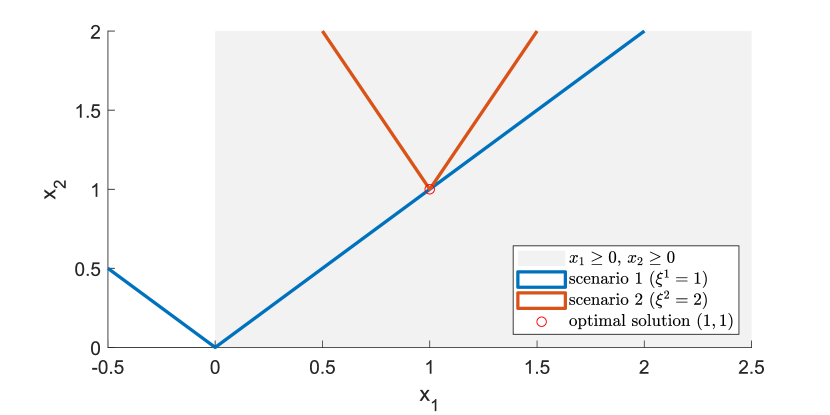
Figure 1: An illustrative example for Lemma 5 and Theorem 5. Constraints of two scenarios are visualized in the figure. The optimal solution is $(1,1)$, which is solely determined by scenario $2$, thus the support set $\operatorname{\mathcal{S}}$ is $\{2\}$. The optimal dual solution is $\mu_{11}=0,\mu_{12}\geq 0$, $\mu_{21}=0.5-0.75\mu_{12}$ and $\mu_{22}=0.5-0.25\mu_{12}$. More details are in Appendix 10.1.

Theorem 5.

Consider a non-degenerate scenario problem $\operatorname{\text{SP}}(\operatorname{\mathcal{N}})$ under Assumptions 2 (feasibility) and 3 (convexity). Let $\mu^{*}:=\{\mu^{i,*}\}_{i=1}^{N}$ denote an optimal dual solution (may not be unique) of $\operatorname{\text{SP}}(\operatorname{\mathcal{N}})$ and define $\mathcal{M}(\mu^{*}):=\{i\in\mathcal{N}:\|\mu^{i,*}\|>0\}$. (1) If $\xi^{j}$ is a support scenario, then $\|\mu^{j,*}\|>0$. In other words, $\operatorname{\mathcal{S}}\subseteq\mathcal{M}(\mu^{*})$ for any optimal dual solution $\mu^{*}$. (2) If $\xi^{j}$ is not a support scenario ($j\notin\operatorname{\mathcal{S}}$), then there exists an optimal dual solution $\mu^{j,*}\in\mathbf{R}_{+}^{m}$ with $\|\mu^{j,*}\|=0$. (3) There exists an optimal dual solution $\mu^{\star}$, such that $\mathcal{M}(\mu^{\star})=\operatorname{\mathcal{S}}$. (4) If the optimal dual solution $\mu^{*}$ is unique, then $\mathcal{M}(\mu^{*})=\operatorname{\mathcal{S}}$.

Remark 3 (The sparsest dual solution $\mu^{\star}$).

In practice, the challenge of applying Theorem 5 is the non-uniqueness of optimal dual solutions. Ideally, we would like to find the dual solution $\mu^{\star}$ that satisfies $\mathcal{M}(\mu^{\star})=\mathcal{S}$. Notice this solution is the sparsest dual solution since all other solutions lead to larger set $\mathcal{M}(\mu^{*})\supseteq\mathcal{S}$. A possible approach is to directly solve the dual of $\operatorname{\text{SP}}(\operatorname{\mathcal{N}})$ with regularizers, instead of solving the primal scenario problem $\operatorname{\text{SP}}(\operatorname{\mathcal{N}})$. The regularization terms are mainly for the purpose of getting sparse solutions. This is part of our ongoing works.

In numerical simulations, the dual solution that an optimization solver returns depends on the choice of algorithm and implementation details. For example, the scenario problem in Figure 1 is non-degenerate according to Definition 3, but there is an infinite number of optimal dual solutions as calculated in Appendix 10.1. We used MOSEK v9.2.9 and GUROBI v9.0.0 to solve the dual of the example in Figure 1. MOSEK returns solution $\mu^{1}=(0,0.3692)$ and $\mu^{2}=(0.2231,0.4077)$, thus $\mathcal{M}=\{1,2\}$. GUROBI returns solution $\mu^{1}=(0,0)$ and $\mu^{2}=(0.5,0.5)$, which is the sparsest solution we prefer.

When the sparsest dual solution is not readily available, we can use Algorithm 1 to identify the support scenarios. Algorithm 1 is based on Definition 2, i.e., checking scenarios in the set $\mathcal{M}(\mu^{*})$ one by one.

1:  Compute the primal and dual solutions $x_{\mathcal{N}}^{*}$ and $\mu^{i,*}$ ($i=1,2,\cdots,N$) by solving $\operatorname{\text{SP}}(\operatorname{\mathcal{N}})$

2:  Let $\mathcal{M}=\{i\in\mathcal{N}:\|\mu^{i,*}\|>0\}$. Set $\mathcal{S}\leftarrow\emptyset$.

3:  for $i\in\mathcal{M}$ do

4:     Solve $\text{SP}_{\mathcal{M}-i}$ and compute $x_{\mathcal{M}-i}^{*}$

5:     if $c^{\intercal}x_{\mathcal{M}-i}^{*}<c^{\intercal}x_{\mathcal{N}}^{*}(=c^{\intercal}x_{\mathcal{M}}^{*})$ then

6:        $\mathcal{S}\leftarrow\mathcal{S}+i$

7:     end if

8:  end for

Algorithm 1 Finding Support Scenarios Using Dual Variables

Remark 4 (Finding the Essential Set For Convex Problems).

If the scenario problem is known to have a unique dual solution, then there is no need to use Algorithm 1. In practice, it is often difficult to know the uniqueness of the solution before solving the problem. So we need to rely on solvers or slightly modify the scenario problem to get the sparsest solution (Theorem 5 and Remark 3). In the worst-case scenario, we compute an optimal dual solution then apply Algorithm 1, which requires us to solve the scenario problem $|\mathcal{M}|$ times. In many cases (especially in power system applications, e.g., [6]), it is observed that the support scenarios are only a small subset of all $N$ scenarios, i.e., $|\mathcal{M}|\approx|\operatorname{\mathcal{S}}|\ll|\operatorname{\mathcal{N}}|$. Comparing with Algorithms 2 or 3, Algorithm 1 only requires solving $\sim|\operatorname{\mathcal{S}}|$ scenario problems, which is much more efficient since $|\operatorname{\mathcal{S}}|\ll|\operatorname{\mathcal{N}}|$.

3.3 Two-stage Scenario Problems

Section 3.1 shows that searching for essential sets can be relatively easier when a scenario problem is non-degenerate. However, finding a support set or irreducible set still requires solving $N$ non-convex problems. Motivated by SCUC, we show that more efficient algorithms are possible by exploiting the structure of specific problems. We study the following two-stage scenario problem in this subsection.

$$\min_{y\in\mathcal{Y}}c_{y}^{\intercal}y+\min_{\begin{subarray}{c}x\in\mathcal{X}\\ (x,y)\in\mathcal{H}\end{subarray}}~{} c_{x}^{\intercal}x$$ (12a)

s.t. $$x\in\cap_{i=1}^{N}\mathcal{U}_{i}$$ (12b)

Constraints on the first-stage variables $y$ and the second-stage variables $x$ are denoted by $y\in\mathcal{Y}$ and $x\in\mathcal{X}$, respectively. Constraint $(x,y)\in\mathcal{H}$ represents the constraints coupling variables $x$ and $y$ in both stages. Set $\mathcal{U}_{i}$ stands for the constraints corresponding to the $i$th scenario $\xi^{i}$.

Problem (12) is an abstract form of s-SCUC in Section 4. Two key features of the two-stage scenario problem are: (1) the non-convexity only comes from constraints $y\in\mathcal{Y}$ (e.g., binary variables in SCUC), all other constraints ($\mathcal{X},\mathcal{H},\mathcal{U}_{i}$) are convex; (2) uncertainties only exist in the second stage.

Let $(x^{*},y^{*})$ be a (possibly local) optimal solution that algorithm $\mathbb{A}$ returns. Given $y=y^{*}$, the second stage problem is convex by setting:

$$\min_{\begin{subarray}{c}x\in\mathcal{X}\\ (x,y^{*})\in\mathcal{H}\end{subarray}}~{} c_{x}^{\intercal}x$$ (13a)

s.t. $$x\in\cap_{i=1}^{N}\mathcal{U}_{i}$$ (13b)

Lemma 6.

(1) Let $\hat{\operatorname{\mathcal{S}}}$ represent the set of support scenarios of (13) and $\operatorname{\mathcal{S}}$ denote the support set for the two-stage problem (12), then $\hat{\operatorname{\mathcal{S}}}\subseteq\operatorname{\mathcal{S}}$; (2) If $\hat{\operatorname{\mathcal{S}}}$ is invariant for (12), i.e., $\operatorname{\text{opt}}_{\mathbb{A}}(\hat{\operatorname{\mathcal{S}}})=\operatorname{\text{opt}}_{\mathbb{A}}(\operatorname{\mathcal{N}})$, then the two-stage scenario problem $\operatorname{\text{SP}}_{\mathbb{A}}(\operatorname{\mathcal{N}})$ is non-degenerate, therefore $\mathcal{S}=\hat{\mathcal{S}}$.

Corollary 2 and Theorem 4 demonstrate many nice properties of non-degenerate scenario problems. Lemma 6 gives a criteria of checking if the two-stage problem (e.g., s-SCUC) is non-degenerate. This lemma lays the foundation of Algorithm 4 to search for essential sets of (12). The main idea of Algorithm 4 is to first find the support scenarios of the second-stage problem (13), then verify if $\operatorname{\text{SP}}(\operatorname{\mathcal{N}})$ is degenerate using Lemma 6. In Section 5.4, it turns out that s-SCUC is non-degenerate in $96\%$ of cases, thus Algorithm 4 could obtain essential sets of s-SCUC (in Section 5.4) in a much shorter time.

4 Security-Constrained Unit Commitment with Probabilistic Guarantees

4.1 Nomenclature

The number of loads, generators, wind farms, transmission lines, contingencies, and snapshots are denoted by $n_{d}$, $n_{g}$, $n_{w}$, $n_{l}$, $n_{k}$ and $n_{t}$, respectively. $\iota\in\{t+1,\cdots,n_{t}\}$

contingency index

time (snapshot) index

additional time (snapshot) index in constraints (14j) and (14k) Binary decision variables (at time $t$): $z^{t}\in\{0,1\}^{n_{g}}$

generator on/off states (commitment)

generator $i$ is on if $u_{i}^{t}=1$

generator $i$ is off if $v_{i}^{t}=1$ Continuous decision variables (at time $t$, contingency $k$): $g^{t,k}\in\mathbf{R}^{n_{g}}$

generation output

reserve Parameters and constants: $a^{k}\in\{0,1\}^{n_{g}}$

generator availability in contingency $k$

weight of contingency $k$

generation costs

no load cost

reserve costs

startup cost

shutdown cost

load forecast (time $t$)

load forecast error (time $t$)

wind forecast (time $t$)

wind forecast error (time $t$)

generation upper bounds

generation lower bounds

ramping upper bounds

ramping lower bounds

minimum on time for generator $i$

minimum off time for generator $i$

4.2 Deterministic SCUC (d-SCUC)

Deterministic security-constrained unit commitment (d-SCUC) (14) seeks optimal commitment and startup/shutdown decisions $(z^{t},u^{t},v^{t})$, generation and reserve schedules $(g^{t,k},r^{t})$ for a horizon of time steps, typically $24$ hours. Security constraints ensures the reliability of the power system after an unexpected event occurs.

$$\min_{z,u,v,g,r}~{} \sum_{t=1}^{n_{t}}\Big{(}c_{z}^{\intercal}z^{t}+c_{u}^{\intercal}u^{t}+c_{v}^{\intercal}v^{t}+c_{r}^{\intercal}r^{t}+\sum_{k=0}^{n_{k}}\alpha_{k}c_{g}^{\intercal}g^{t,k}\Big{)}$$ (14a)

s.t. $$\mathbf{1}^{\intercal}g^{t,k}+\mathbf{1}^{\intercal}\hat{w}^{t}\geq\mathbf{1}^{\intercal}\hat{d}^{t}$$ (14b)

$$\underline{f}\leq H_{g}^{t,k}g^{t,k}+H_{w}^{t,k}w^{t,k}-H_{d}^{t,k}d^{t,k}\leq\overline{f}$$ (14c)

$$a^{k}\circ\underline{\gamma}\leq g^{t,k}-g^{t-1,k}\leq a^{k}\circ\overline{\gamma}$$ (14d)

$$a^{k}\circ(g^{t,0}-r^{t})\leq g^{t,k}\leq a^{k}\circ(g^{t,0}+r^{t})$$ (14e)

$$\hskip 109.0ptk\in[0,n_{k}],t\in[1,n_{t}]$$

$$\underline{g}\circ z^{t}\leq g^{t,0}\leq\overline{g}\circ z^{t}$$ (14f)

$$\underline{g}\circ z^{t}\leq g^{t,0}-r^{t}\leq g^{t,0}+r^{t}\leq\overline{g}\circ z^{t}$$ (14g)

$$z^{t-1}-z^{t}+u^{t}\geq 0$$ (14h)

$$z^{t}-z^{t-1}+v^{t}\geq 0$$ (14i)

$$\hskip 157.0ptt\in[1,n_{t}]$$

$$z_{i}^{t}-z_{i}^{t-1}\leq z_{i}^{\iota},~{}i\in[1,n_{g}]$$ (14j)

$$\hskip 23.0pt\iota\in[t+1,\min\{t+\underline{u}_{i}-1,n_{t}\}],t\in[2,n_{t}]$$

$$z_{i}^{t-1}-z_{i}^{t}\leq 1-z_{i}^{\iota},~{}i\in[1,n_{g}]$$ (14k)

$$\hskip 23.0pt\iota\in[t+1,\min\{t+\underline{v}_{i}-1,n_{t}\}],t\in[2,n_{t}]$$

The objective of (14) is to minimize total operation costs, including no-load costs $c_{z}^{\intercal}z^{t}$, startup costs $c_{u}^{\intercal}u^{t}$, shutdown costs $c_{v}^{\intercal}v^{t}$, generation costs $c_{g}^{\intercal}g^{t,k}$ and reserve costs $c_{r}^{\intercal}s^{t}$. Security constraints ensure: enough supply to meet demand (14b), transmission line flow within limits (14c), generation levels within ramping limits (14d) and capacity limits (14f) in any contingency $k$. Constraints (14e) and (14g) are about the relationship between generation and reserve in any contingency $k$. Constraints (14h)-(14i) are the logistic constraints about commitment status, startup and shutdown decisions. Minimum on/off time constraints for all generators are in (14j)-(14k). Constraints (14d)-(14g) also guarantee the consistency of generation levels $g^{t,k}$ with commitment decisions $z^{t}$ and generator availability $a^{k}$ in contingency $k$ [32].

To reveal the structure of d-SCUC, we define the sets below:

$$\mathcal{B} :=\big{\{}(z,u,v):\eqref{opt:det-SCUC-startup},\eqref{opt:det-SCUC-shutdown},\eqref{opt:det-SCUC-minon-time},\eqref{opt:det-SCUC-minoff-time}\big{\}}$$ (15a)

$$\mathcal{C} :=\big{\{}(g,r):\eqref{opt:det-SCUC-balance},\eqref{opt:det-SCUC-line},\eqref{opt:det-SCUC-ramp},\eqref{opt:det-SCUC-contingency}\big{\}}$$ (15b)

$$\mathcal{H} :=\big{\{}(z,g,r):\eqref{opt:det-SCUC-gencap},\eqref{opt:det-SCUC-resgencap}\big{\}}$$ (15c)

Sets $\mathcal{B}$ and $\mathcal{C}$ stand for the deterministic constraints for binary and continuous variables, respectively. Set $\mathcal{H}$ represents the hybrid constraints related with both continuous and binary variables. Then d-SCUC can be succinctly represented as

$$\min_{z,u,v,g,r}~{} \eqref{opt:det-SCUC-obj}$$

s.t. $$(z,u,v)\in\mathcal{B},~{}(g,r)\in\mathcal{C},~{}(z,g,r)\in\mathcal{H}$$

4.3 Chance-constrained SCUC (c-SCUC)

The d-SCUC formulation utilizes the expected wind generation and load forecast, it does not take the uncertainties from wind and load into consideration. Various formulations of chance-constrained SCUC (c-SCUC) have been proposed, e.g., [33, 34]. The c-SCUC formulations explicitly guarantee the system security with a tunable level of risk $\epsilon$ with respect to uncertainties. Instead of using expected load $\hat{d}^{t}$ as in (14), we consider loads $d^{t}$ as forecast $\hat{d}^{t}$ plus a random forecast error $\tilde{d}^{t}$ (i.e., $d^{t}=\hat{d}^{t}+\tilde{d}^{t}$).

$$\mathbb{P}_{\tilde{w}\times\tilde{d}}\Big{(}\mathbf{1}^{\intercal}g^{t,k}+\mathbf{1}^{\intercal}(\hat{w}^{t}+\tilde{w}^{t})\geq\mathbf{1}^{\intercal}(\hat{d}^{t}+\tilde{d}^{t}),\\ \underline{f}\leq H_{g}^{t,k}g^{t,k}+H_{w}^{t,k}(\hat{w}^{t}+\tilde{w}^{t})-H_{d}^{t,k}(\hat{d}^{t}+\tilde{d}^{t})\leq\overline{f},\\ k\in[0,n_{k}],t\in[1,n_{t}]\Big{)}\geq 1-\epsilon$$ (16)

We define set $\mathcal{U}:=\{g:\eqref{opt:chance-constrained-in-SCUC}\}$ to represent all constraints related with uncertainties. Then the formulation of chance-constrained Security-constrained Unit Commitment (c-SCUC) is presented below. Comparing with d-SCUC, the only difference of c-SCUC is the addition of the chance constraint (16). The chance constraint guarantees there will be enough supply to meet the net demand with probability no less than $1-\epsilon$.

$$\min_{z,u,v,g,r}~{} \eqref{opt:det-SCUC-obj}$$

s.t. $$(z,u,v)\in\mathcal{B},~{}(g,r)\in\mathcal{C},~{}(z,g,r)\in\mathcal{H}$$

$$\mathbb{P}\big{(}g\in\mathcal{U}\big{)}\geq 1-\epsilon$$

4.4 Scenario-based SCUC (s-SCUC)

The scenario approach was mainly targeted at convex problems (see Assumption 3), whereas SCUC is non-convex by nature due to on/off commitment decisions. Consequently, the scenario approach was considered not applicable for c-SCUC. An extended version of the scenario approach was proposed recently in [29], which makes it applicable for non-convex problems such as SCUC. Another related paper is in [35], which applies Theorem 3 on the AC optimal power flow problem and obtain similar posterior guarantees.

Using the scenario approach, c-SCUC is approximated by the scenario-based SCUC (s-SCUC) problem below:

$$\min_{(z,u,v)\in\mathcal{B}}~{} \sum_{t=1}^{n_{t}}\Big{(}c_{z}^{\intercal}z^{t}+c_{u}^{\intercal}u^{t}+c_{v}^{\intercal}v^{t}\Big{)}+$$

$$\min_{(z,g,r)\in\mathcal{H}}\sum_{t=1}^{n_{t}}\Big{(}c_{r}^{\intercal}r^{t}+\sum_{k=0}^{n_{k}}\alpha_{k}c_{g}^{\intercal}g^{t,k}\Big{)}$$

$$\hskip 28.45274pt\text{s.t.}~{}(g,r)\in\mathcal{C}$$

$$\hskip 42.67912ptg\in\cap_{i=1}^{N}\mathcal{U}_{i}$$

Remark 5.

SCUC is a two-stage optimization problem by nature, it has the following nice properties. Firstly, the non-convexity only exists in the first stage, i.e., $y\in\mathcal{Y}$. Given a first-stage solution $y$, the second stage is a simple linear program. Secondly, uncertainties come from renewables in the operation stage (only in the second stage). Based on the nice structural properties above, Section 3.3 shows that we are able to track down essential sets by solving two MILPs and $\sim|\operatorname{\mathcal{S}}|$ linear programs.

4.5 Degeneracy of s-SCUC

This section presents an example to show that s-SCUC could be degenerate in many cases, which violates Assumption 1. Therefore almost all results of the classical scenario approach are not applicable. For s-SCUC, theoretical guarantees are only possible through the non-convex scenario approach in Section 2.3.

We use a 3-bus system to illustrate the degeneracy of s-SCUC. Configurations of the 3-bus system are in [36]. In order to visualize the feasible region of s-SCUC, we simplify the problem by (1) only considering one snapshot ($n_{t}=1$) and ignoring initial status (thus no $u,v$ variables); (2) removing reserve constraints (no $r$ variables). By doing this, there are only four decision variables left: $z_{1},z_{2},g_{1},g_{2}$. The on/off states $z_{1},z_{2}$ can be inferred from values of $g_{1}$ and $g_{2}$, therefore the feasible region of the simplified s-SCUC can be visualized on the $(g_{1},g_{2})$-plane.

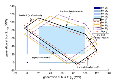
(a) Illustration of the feasible region with constraints of all scenarios ($\mathcal{U}_{1}$,$\mathcal{U}_{2}$,$\mathcal{U}_{3}$).

(b) Illustration of the feasible region with only support scenarios ($\mathcal{U}_{1}$).

Figure 2: An illustrative example that s-SCUC is degenerate (3-bus system)

Using Definition 3, showing the degeneracy of s-SCUC includes three steps: (1) obtaining the optimal solution to $\operatorname{\text{SP}}(\operatorname{\mathcal{N}})$; (2) finding all support scenarios $\operatorname{\mathcal{S}}$ of $\operatorname{\text{SP}}(\operatorname{\mathcal{N}})$; and (3) checking if the optimal solution of $\operatorname{\text{SP}}(\operatorname{\mathcal{N}})$ is the same as $\operatorname{\text{SP}}(\operatorname{\mathcal{S}})$. Fig. 2a first visualizes constraints $\mathcal{B}_{0}\sim\mathcal{B}_{3}$, which represents the region of 4 possible generator on/off status (e.g., $\mathcal{B}_{1}:z_{1}=1,z_{2}=0$, $\mathcal{B}_{3}:z_{1}=1,z_{2}=1$). The black solid lines denote constraints (14b), (14c) and (14f) using forecast values (d-SCUC). The red, yellow and purple dotted lines are three sets ($\mathcal{U}_{1},\mathcal{U}_{2},\mathcal{U}_{3}$) of constraints corresponding to three scenarios. Given the setting that generator 1 is much cheaper than generator 2, we can easily eyeball the optimal solution with all constraints presented, marked by the red $*$. Next, we observe that removing scenario 1 ($\mathcal{U}_{1}$, red lines) changes the optimal solution, while removing scenario scenario 2 ($\mathcal{U}_{2}$, yellow lines) or scenario 3 ($\mathcal{U}_{3}$, purple lines) makes no difference. Thus scenario 1 is the only support scenario. Finally, we examine the scenario problem with only support scenarios presented. Fig. 2b shows that the optimal solution becomes the red $\diamond$ with only scenario 1, which is clearly different than the optimal solution in Fig. 2a. Hence, s-SCUC is a degenerate problem.

5 Numerical Results

5.1 Settings of the 118-bus System

Numerical simulations were conducted on a modified 118-bus, 184-line, 54-generator, 24-hour system [37]. Most settings are identical as [37], except 5 wind farms are added to the system as in [38]. The s-SCUC problems were solved using $64$ GB memory on the Hera server (hera.ece.tamu.edu), provided by Texas A&M University. The mathematical models for s-SCUC was formulated using YALMIP [39] on Matlab R2019a and solved using Gurobi v8.1 [40].

After obtaining a solution $\operatorname{\text{opx}}_{\mathbb{A}}(\operatorname{\mathcal{N}})$ to s-SCUC, Theorem 3 provides an upper bound $\epsilon(N,|\operatorname{\mathcal{I}}|,\beta)$ on the actual violation probability $\mathbb{V}(\operatorname{\text{opx}}_{\mathbb{A}}(\operatorname{\mathcal{N}}))$. The theoretical guarantee $\epsilon(N,|\operatorname{\mathcal{I}}|,\beta)$ is referred as posterior $\epsilon$ in the numerical results. The actual violation probability $\mathbb{V}(\operatorname{\text{opx}}_{\mathbb{A}}(\operatorname{\mathcal{N}}))$ is estimated by the out-of-sample violation probability $\hat{\epsilon}$, using an independent set of $10^{6}$ scenarios.

To quantify the randomness of the scenario approach, for each sample complexity $N=100,200,\cdots,1000$, we solve the corresponding s-SCUC problems on 10 independent sets of scenarios (i.e., $10$ Monte-Carlo simulations). Results in both Fig. 3 and 4 show the average, maximum and minimum values in 10 Monte-Carlo simulations.

5.2 Cost vs Security: a trade-off

Fig. 3 shows the out-of-sample violation probability $\hat{\epsilon}$ and objective value (total cost). The shadowed area shows the max-min values in 10 Monte-Carlo simulations, and the solid line is the average value. It is shown that the system risk level (violation probability) is reduced by $83\%$ (from $\sim 30\%$ to $\sim 5\%$) by $\sim 1.1\%$ increase in total system costs. Similar observations were found in [6, 3, 32].

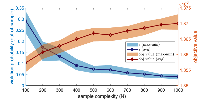
Figure 3: Cost vs Security: a Trade-off.

5.3 Violation Probability

Fig. 4 presents the out-of-sample violation probability $\hat{\epsilon}$ and theoretical guarantees (posterior $\epsilon$ provided by Theorem 3). Since the cardinality of essential sets differ for each scenario problem (Fig. 5), the posterior guarantee $\epsilon$ is a band instead of a line. As illustrated in Fig. 4, the actual violation probability (approximated by $\hat{\epsilon}$) is bounded by the theoretical guarantees. This verifies the correctness of Theorem 3. The conservative ratio is $2\sim 4$ (e.g., when out-of-sample $\hat{\epsilon}$ is $\sim 5\%$, Theorem 3 gives an upper bound $10\%\sim 20\%$).

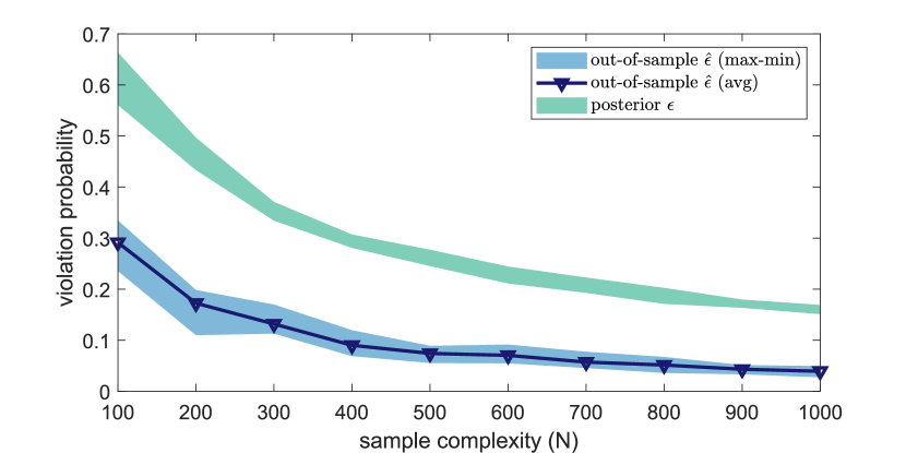
Figure 4: Out-of-sample Violation Probabilities and Theoretical Guarantees.

5.4 Searching for Essential Sets for s-SCUC

s-SCUC was observed to be non-degenerate in 192 out of 200 simulations. In other words, in $96\%$ cases, we are able to find an essential set by solving $5\sim 35$ linear programs and $2$ mixed integer linear programs. It takes from 4934 seconds ($N=100$) to 6847 seconds ($N=1000$) to solve one MILP (s-SCUC). When searching for support scenarios for the second-stage problem (a linear program), it takes $281\sim 388$ seconds to solve one LP. For those 8 out of 200 simulations, it takes an extra $20$ hours to find an irreducible set using Algorithm 2. This computation time can be greatly reduced by tricks such as choosing appropriate starting points.

6 Discussions

6.1 Cardinality of Essential Sets

Fig. 5 compares the cardinalities of essential sets for three cases: (a) c-SCUC with $N-1$ contingencies but without transmission constraints, results of case (a) are obtained from [32]); (b) c-SCUC with transmission constraints but without $N-1$ contingencies; and (c) c-SCUC with both transmission constraints and $N-1$ contingencies.

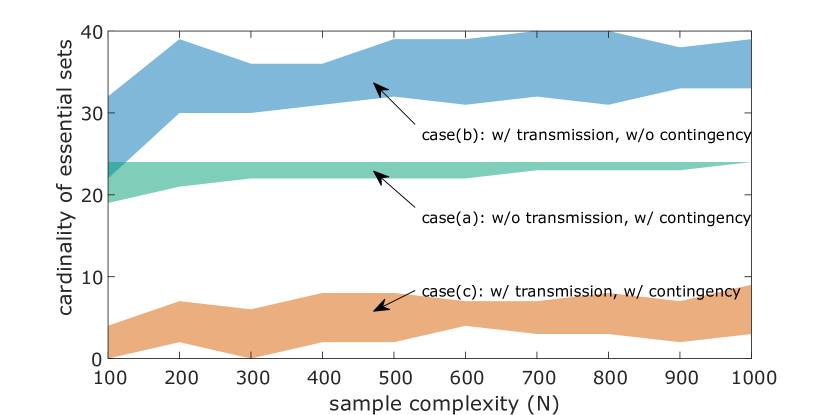
Figure 5: Cardinality of Essential Sets.

Case (a) is the simplest, in [32] we show that the scenario problem for unit commitment satisfies the non-degeneracy assumption 1, and the cardinality of essential sets is bounded by the number of snapshots $n_{t}$, i.e., $|\operatorname{\mathcal{S}}|\leq n_{t}=24$ in Fig. 5. Cases (b) and (c) include transmission capacity constraints. As demonstrated in Section 4.5, s-SCUC could be degenerate with transmission constraints. Theoretically speaking, the cardinality of essential sets might be unbounded for non-convex problems. Fig. 5 shows that the cardinality of essential sets is greatly smaller than the number of decision variables. For example, s-SCUC has about $4000$ binary variables and around $75000$ continuous decision variables, while the cardinalities of essential sets are $30\sim 40$ in case (b) and $0\sim 10$ in case (c). This observation implies that the number of scenarios $N$ required could be much smaller than expected.

Another interesting observation is that including $N-1$ contingency constraints reduces $|\operatorname{\mathcal{E}}|$. This observation has two implications. First, $N-1$ contingency constraints not only protect the system from unexpected device failures, they also help reduce the impacts of uncertainties from renewables. Second, including $N-1$ contingency constraints could help reduce sample complexity. Similar with the observations in [6], this observation indicates that the scenario approach might be of practical use.

6.2 From Posterior to Prior Guarantees

Theorem 3 gives posterior guarantees on the feasibility of solutions, namely, we calculate $\epsilon(N,k,\beta)$ after obtaining the solution $\operatorname{\text{opx}}(\operatorname{\mathcal{N}})$. Lemma 1 proves that the $\epsilon(N,k,\beta)$ function in (9) is monotone in $N$ and $k$. This implies that we can obtain prior guarantees. In other words, if the cardinality of essential sets is proved to be at most $h$ ($|\operatorname{\mathcal{E}}|\leq h$), then we can compute the smallest $\hat{N}$ (e.g., using binary search) such that $\epsilon\geq 1-\Big{(}\frac{\beta}{\hat{N}\binom{\hat{N}}{h}}\Big{)}^{\frac{1}{\hat{N}-h}}$ holds for given $\epsilon$ and $\beta$. Then the solution $\operatorname{\text{opx}}_{\mathbb{A}}(\operatorname{\mathcal{N}})$ to the scenario problem using $\hat{N}$ scenarios has the guarantee $\mathbb{P}(\mathbb{V}(\operatorname{\text{opx}}_{\mathbb{A}}(\operatorname{\mathcal{N}}))\leq\epsilon)\geq 1-\beta$. This prior guarantee holds before solving the scenario problem with $\hat{N}$ scenarios. If a rigorous bound $h$ on $|\operatorname{\mathcal{E}}|$ can be proved, then there is no need to numerically search for essential sets. This is particularly attractive compared with posterior guarantees. One example is the chance-constrained unit commitment (without transmission line limits) in [32], in which we show that the cardinality of essential sets is bounded by the number of snapshots $n_{t}$, i.e., $|\operatorname{\mathcal{S}}|\leq n_{t}=24$, also shown in case (a) of Fig. 5. Although general non-trivial bounds on $|\operatorname{\mathcal{E}}|$ may not exist, results of [32] indicate that bounding $|\operatorname{\mathcal{E}}|$ is possible for structured non-convex problems.

6.3 Optimality Gap vs Violation Probability

Unlike Theorem 1, which only holds for the global optimal solution, the non-convex scenario approach theory (Theorem 3) works for any feasible solution to the scenario problem. In Figs. 6 and 7, we compare the performance of a suboptimal solution with the optimal solution (MIP Gap less than $0.01\%$) in Section 5.2. The suboptimal solution is obtained by fixing all $z_{i}^{t}=1,u_{i}^{t}=0,v_{i}^{t}=0,\forall i,\forall t$ and solve the s-SCUC problem. In other words, the suboptimal solution does not take the optimal commitment of generators into account, it only optimizes the dispatch $(g,r)$ variables.

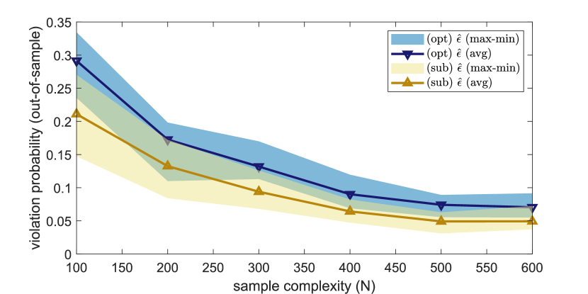
Figure 6: Out-of-sample Violation Probabilities of the Optimal Solution (opt) and a Suboptimal Solution (sub)

Fig. 6 compares the out-of-sample violation probabilities. Using the same number of scenarios $N$, suboptimal solutions always have smaller violation probabilities (more secure or conservative). If violation probabilities of solutions are guaranteed to be acceptable ranges, then we should always pursue the optimal solution with smaller objective values to reduce conservativeness.

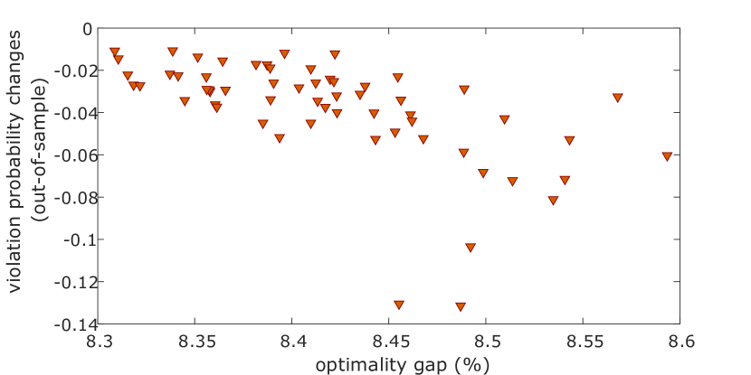
Figure 7: Optimality Gap vs Violation Probability. 60 dots in this figure represent 60 instances of s-SCUC solved.

Fig. 7 further examines the relationship between optimality and security. The x-axis is the optimality gap, i.e., the percentage differences between suboptimal solutions and optimal solutions. The y-axis is the difference between violation probabilities of suboptimal and optimal solutions. Negative values indicate that violation probabilities of suboptimal solutions are always smaller than those of optimal solutions. There is also a subtle trend that larger optimality gaps lead to bigger decrease in violation probabilities.

7 Concluding Remarks

This paper studies a core problem in the scenario approach theory, i.e., efficiently identifying essential sets for general scenario problems. For convex problems, we prove that the sparsest dual solution of the scenario problem could pinpoint the essential set. For non-convex problems, we provide conditions where simple algorithms based on definitions could return the essential set when the scenario problem is non-degenerate. We use chance-constrained Security-constrained Unit Commitment as a numerical example. Case studies on an IEEE benchmark system show that the essential scenario set is only a small subset of all scenarios. This implies that we can obtain relatively robust solutions (i.e., small $\epsilon$) using only a moderate number of scenarios. Furthermore, we observe that some power engineering practices (e.g., $N-1$ criteria) can help us reduce the number of scenarios needed while maintaining the same level of risk.

Future work includes (1) reducing conservativeness by improving the complexity bound in Theorem 3; (2) a more systematic approach to compute the sparsest dual solution of convex scenario problems; and (3) investigating the performance of the (non-convex) scenario approach on larger-scale realistic power systems.

8 Proofs

The proof of Lemma 1 is through basic inequalities, we omitted it to meet the length requirement (max 13 pages). Complete details about the proof of Lemma 1 is available in the supplementary material and at [36].

Proof of Lemma 2 [27].

For the purpose of contradiction, we assume that there is a scenario $s\in\operatorname{\mathcal{S}}$ but $s\notin\operatorname{\mathcal{I}}$. According to the definition of support scenarios, $\operatorname{\text{opt}}_{\mathbb{A}}(\operatorname{\mathcal{N}}-s)<\operatorname{\text{opt}}_{\mathbb{A}}(\operatorname{\mathcal{N}})$. However, Assumption 4 claims that removing scenarios will not increase the optimal objective value and $\operatorname{\mathcal{I}}\subseteq\operatorname{\mathcal{N}}-s$, we have $\operatorname{\text{opt}}_{\mathbb{A}}(\operatorname{\mathcal{N}}-s)\geq\operatorname{\text{opt}}_{\mathbb{A}}(\operatorname{\mathcal{I}})=\operatorname{\text{opt}}_{\mathbb{A}}(\operatorname{\mathcal{N}})$, which causes a contradiction. ∎

Proof of Lemma 3.

$k\notin\operatorname{\mathcal{S}}$ and $s\in\operatorname{\mathcal{S}}$ give $\operatorname{\text{opt}}(\operatorname{\mathcal{N}}-k)=\operatorname{\text{opt}}(\operatorname{\mathcal{N}})$ and $\operatorname{\text{opt}}(\operatorname{\mathcal{N}}-s)<\operatorname{\text{opt}}(\operatorname{\mathcal{N}})$, respectively. Assumption 4 shows $\operatorname{\text{opt}}(\operatorname{\mathcal{N}}-k-s)\leq\operatorname{\text{opt}}(\operatorname{\mathcal{N}}-s)$. Hence, it holds that

$$\operatorname{\text{opt}}(\operatorname{\mathcal{N}}-k-s)\leq\operatorname{\text{opt}}(\operatorname{\mathcal{N}}-s)<\operatorname{\text{opt}}(\operatorname{\mathcal{N}})=\operatorname{\text{opt}}(\operatorname{\mathcal{N}}-k),\forall s\in\operatorname{\mathcal{S}}(\operatorname{\mathcal{N}})$$

then $s$ is a support scenario for $\operatorname{\text{SP}}(\operatorname{\mathcal{N}}-k)$, thus $\operatorname{\mathcal{S}}(\operatorname{\mathcal{N}})\subseteq\operatorname{\mathcal{S}}(\operatorname{\mathcal{N}}-k)$. ∎

Proof of Lemma 5.

For the purpose of contradiction, we assume $i\in\mathcal{S}\cap\mathcal{P}$. Since $i$ is a support scenario, there is a new optimal solution $x_{\mathcal{N}-i}^{*}$ with $c^{\intercal}x_{\mathcal{N}-i}^{*}<c^{\intercal}x_{\mathcal{N}}^{*}$. Let $0<\alpha<1$ be a positive number, and we consider the solution $\hat{x}=\alpha x_{\mathcal{N}-i}^{*}+(1-\alpha)x_{\mathcal{N}}^{*}$. It is obvious that

$$c^{\intercal}\hat{x}<\alpha c^{\intercal}x_{\mathcal{N}}^{*}+(1-\alpha)c^{\intercal}x_{\mathcal{N}}^{*}=c^{\intercal}x_{\mathcal{N}}^{*}$$

Next we show that $\hat{x}$ is feasible to $\operatorname{\text{SP}}(\operatorname{\mathcal{N}})$ if $\alpha$ is small enough. Since $i\in\mathcal{P}$, there exists a positive number $\delta$ such that $f(x_{\mathcal{N}}^{*},\xi^{i})\leq-\delta$. Using the fact that $f(x,\xi)$ is convex in $x$ and convex functions are also Lipschitz (with Lipschitz constant $L$), we can derive an upper bound $\overline{\alpha}(L,\delta)$, such that for any $0<\alpha\leq\overline{\alpha}(L,\delta)$, we have $f(x_{\operatorname{\mathcal{N}}}^{*},\xi^{i})\leq-\delta\leq f(\hat{x},\xi^{i})\leq 0$. For other constraints $f(x,\xi^{j})\leq 0$ ($j\neq i$), it is easy to see that $\hat{x}$ is also feasible because it is the convex combination of two feasible points. Therefore $\hat{x}$ is another feasible solution to $\operatorname{\text{SP}}(\operatorname{\mathcal{N}})$ but with smaller objective $c^{\intercal}\hat{x}<c^{\intercal}x_{\mathcal{N}}^{*}$. This causes contradiction. ∎

Proof of Theorem 5.

(Preparation) The Lagrange dual function $D_{\operatorname{\mathcal{N}}}(\mu,\lambda)$ of $\operatorname{\text{SP}}(\operatorname{\mathcal{N}})$ is:

$$D_{\operatorname{\mathcal{N}}}(\mu,\lambda)=\inf_{x}\Big{(}c^{\intercal}x+\sum_{\iota=1}^{N}(\mu^{\iota})^{\intercal}f(x,\xi^{\iota})+\lambda^{\intercal}g(x)\Big{)}$$ (17)

The Lagrange dual problem is $\max_{\mu\geq 0,\lambda\geq 0}D_{\operatorname{\mathcal{N}}}(\mu,\lambda)$, and we use $\lambda_{\operatorname{\mathcal{N}}}^{*}$ and $\mu_{\operatorname{\mathcal{N}}}^{*}=\{\mu_{\operatorname{\mathcal{N}}}^{i,*}\}_{i=1}^{N}$ to denote its optimal solution. By Assumption 2 (feasibility), we know that $\operatorname{\text{SP}}(\operatorname{\mathcal{N}})$ has a strictly feasible solution, thus Slater’s condition holds and $D(\mu_{\mathcal{N}}^{*},\lambda_{\mathcal{N}}^{*})=c^{\intercal}x_{\mathcal{N}}^{*}$ by strong duality. We then consider the Lagrange dual problem of $\operatorname{\text{SP}}(\operatorname{\mathcal{N}}-j)$. Instead of directly removing constraints $f(x,\xi^{j})\leq 0$, we consider the following relaxed version

$$f(x,\xi^{j})\leq M\mathbf{1}.$$ (18)

When constant $M$ is sufficiently large, it is as if constraints $f(x,\xi^{j})\leq 0$ are removed. The associated dual problem is

$$D_{\operatorname{\mathcal{N}}-j}(\mu,\lambda)=D_{\operatorname{\mathcal{N}}}(\mu,\lambda)-M\mathbf{1}^{\intercal}\mu^{j}$$ (19)

The optimal dual solution of $\operatorname{\text{SP}}(\operatorname{\mathcal{N}}-j)$ is denoted by $\lambda_{\operatorname{\mathcal{N}}-j}^{*}$ and $\mu_{\operatorname{\mathcal{N}}-j}^{*}=\{\mu_{\operatorname{\mathcal{N}}-j}^{i,*}\}_{i=1}^{N}$. Note that $\|\mu_{\operatorname{\mathcal{N}}-j}^{j,*}\|=0$, otherwise $D_{\operatorname{\mathcal{N}}-j}(\mu,\lambda)$ will be dominated by $M\mathbf{1}^{\intercal}\mu^{j}$, which is unbounded when $M$ is arbitrarily large, which leads to contradiction.

We first prove (1). For the purpose of contradiction, we assume $j$ is a support scenario but with $\|\mu_{\operatorname{\mathcal{N}}}^{j,*}\|=0$. Since $j$ is a support scenario, from strong duality, we know that

$$D_{\operatorname{\mathcal{N}}}(\mu_{\operatorname{\mathcal{N}}}^{*},\lambda_{\operatorname{\mathcal{N}}}^{*})=c^{\intercal}x_{\operatorname{\mathcal{N}}}^{*}>c^{\intercal}x_{\operatorname{\mathcal{N}}-j}^{*}=D_{\operatorname{\mathcal{N}}-j}(\mu_{\operatorname{\mathcal{N}}-j}^{*},\lambda_{\operatorname{\mathcal{N}}-j}^{*})$$

If $\|\mu_{\operatorname{\mathcal{N}}}^{j,*}\|=0$, then $(\lambda_{\operatorname{\mathcal{N}}}^{*},\mu_{\operatorname{\mathcal{N}}}^{*})$ is a feasible solution to $\max_{\mu\geq 0,\lambda\geq 0}D_{\operatorname{\mathcal{N}}-j}(\mu,\lambda)$, therefore

$$D_{\operatorname{\mathcal{N}}-j}(\mu_{\operatorname{\mathcal{N}}-j}^{*},\lambda_{\operatorname{\mathcal{N}}-j}^{*})\geq D_{\operatorname{\mathcal{N}}-j}(\mu_{\operatorname{\mathcal{N}}}^{*},\lambda_{\operatorname{\mathcal{N}}}^{*})\\ =D_{\operatorname{\mathcal{N}}}(\mu_{\operatorname{\mathcal{N}}}^{*},\lambda_{\operatorname{\mathcal{N}}}^{*})-M\mathbf{1}^{\intercal}\mu_{\operatorname{\mathcal{N}}}^{j,*}=D_{\operatorname{\mathcal{N}}}(\mu_{\operatorname{\mathcal{N}}}^{*},\lambda_{\operatorname{\mathcal{N}}}^{*})\\ >D_{\operatorname{\mathcal{N}}-j}(\mu_{\operatorname{\mathcal{N}}-j}^{*},\lambda_{\operatorname{\mathcal{N}}-j}^{*})$$

which is a contradiction.

Next we prove (2) by constructing an optimal dual solution with $\|\mu^{j,*}\|=0$. If $\xi^{j}$ is not a support scenario, then

$$D_{\operatorname{\mathcal{N}}}(\mu_{\operatorname{\mathcal{N}}}^{*},\lambda_{\operatorname{\mathcal{N}}}^{*})=c^{\intercal}x_{\operatorname{\mathcal{N}}}^{*}=c^{\intercal}x_{\operatorname{\mathcal{N}}-j}^{*}=D_{\operatorname{\mathcal{N}}-j}(\mu_{\operatorname{\mathcal{N}}-j}^{*},\lambda_{\operatorname{\mathcal{N}}-j}^{*})$$ (20)

by Slater’s condition and strong duality. We could assign $\hat{\mu}_{\operatorname{\mathcal{N}}}^{\iota,*}=\mu_{\operatorname{\mathcal{N}}-j}^{\iota,*}$ for $\iota\neq j$ and let $\hat{\mu}_{\operatorname{\mathcal{N}}}^{j,*}=\mathbf{0}$. For the constructed solution $\hat{\mu}_{\operatorname{\mathcal{N}}}^{*}$, we have

$$D_{\operatorname{\mathcal{N}}}(\hat{\mu}_{\operatorname{\mathcal{N}}}^{*},\lambda_{\operatorname{\mathcal{N}}-j}^{*})=D_{\operatorname{\mathcal{N}}-j}(\mu_{\operatorname{\mathcal{N}}-j}^{*},\lambda_{\operatorname{\mathcal{N}}-j}^{*})=c^{\intercal}x_{\operatorname{\mathcal{N}}}^{*}$$

Clearly this is one optimal dual solution to $\operatorname{\text{SP}}(\operatorname{\mathcal{N}})$.

Next we prove (3). First, we solve the dual problem of $\operatorname{\text{SP}}(\operatorname{\mathcal{S}})$ (with support scenarios only) and obtain optimal solution $(\lambda_{\operatorname{\mathcal{S}}}^{*},\mu_{\operatorname{\mathcal{S}}}^{*})$. Note that $\|\mu_{\mathcal{S}}^{\iota,*}\|>0$ for any $\iota\in\mathcal{S}$ according to (1). Next, we assign $\mu_{\operatorname{\mathcal{N}}}^{\iota,*}=\mu_{\operatorname{\mathcal{S}}}^{\iota,*}$ for $\iota\in\operatorname{\mathcal{S}}$, and assign $\mu_{\operatorname{\mathcal{N}}}^{\iota,*}=\mathbf{0}$ for $\iota\notin\operatorname{\mathcal{S}}$. Similar to the proof of (2), this constructed solution $(\lambda_{\operatorname{\mathcal{S}}}^{*},\mu_{\operatorname{\mathcal{N}}}^{*})$ is an optimal dual solution to $\operatorname{\text{SP}}(\operatorname{\mathcal{N}})$. With this constructed $\mu_{\operatorname{\mathcal{N}}}^{*}$, we know that $\mathcal{M}(\mu_{\operatorname{\mathcal{N}}}^{*})\subseteq\operatorname{\mathcal{S}}$. Combining with the claim $\operatorname{\mathcal{S}}\subseteq\mathcal{M}(\mu_{\operatorname{\mathcal{N}}}^{*})$ in (1), we have $\mathcal{M}(\mu_{\operatorname{\mathcal{N}}}^{*})=\operatorname{\mathcal{S}}$.

(4) is obvious from (3). ∎

Proof of Corollary 2.

We first prove (1), that is $\operatorname{\text{SP}}(\operatorname{\mathcal{N}})$ has a unique essential set if it is non-degenerate (similar with the proof of Lemma 2.11 in [27])). From Lemma 2, an essential set can be written as $\operatorname{\mathcal{E}}=\operatorname{\mathcal{S}}\cup\mathcal{Y}$ where $\mathcal{Y}\subseteq(\operatorname{\mathcal{N}}-\operatorname{\mathcal{S}})$. The support set $\operatorname{\mathcal{S}}$ is invariant because of the non-degeneracy of $\operatorname{\text{SP}}(\operatorname{\mathcal{N}})$ by assumption. Since $\operatorname{\mathcal{E}}$ is the invariant set of minimal cardinality, we can let $\mathcal{Y}=\emptyset$ and $\operatorname{\mathcal{S}}$ is the essential set. The support set $\operatorname{\mathcal{S}}$ is unique by definition, this implies the uniqueness of the essential set $\operatorname{\mathcal{E}}$ for non-degenerate $\operatorname{\text{SP}}(\operatorname{\mathcal{N}})$.

We then prove (2). Lemma 2 shows that $\operatorname{\mathcal{S}}\subseteq\operatorname{\mathcal{R}}$, we only need to show $\operatorname{\mathcal{R}}\subseteq\operatorname{\mathcal{S}}$ when $\operatorname{\text{SP}}_{\mathbb{A}}(\operatorname{\mathcal{N}})$ is non-degenerate. For the purpose of contradiction, we assume there exists $s\in\operatorname{\mathcal{R}}$ but $s\notin\operatorname{\mathcal{S}}$. By hypothesis ($s\notin\operatorname{\mathcal{S}}$), we have $\operatorname{\mathcal{S}}\subseteq\operatorname{\mathcal{R}}-s$ (Lemma 2). The monotonicity assumption 4 gives $\operatorname{\text{opt}}_{\mathbb{A}}(\operatorname{\mathcal{S}})\leq\operatorname{\text{opt}}_{\mathbb{A}}(\operatorname{\mathcal{R}}-s)$. Since $\operatorname{\mathcal{R}}$ is irreducible, we have $\operatorname{\text{opt}}_{\mathbb{A}}(\operatorname{\mathcal{R}}-s)<\operatorname{\text{opt}}_{\mathbb{A}}(\operatorname{\mathcal{R}})$. $\operatorname{\text{SP}}_{\mathbb{A}}(\operatorname{\mathcal{N}})$ is non-degenerate and $\operatorname{\mathcal{R}}$ is invariant gives $\operatorname{\text{opt}}_{\mathbb{A}}(\operatorname{\mathcal{R}})=\operatorname{\text{opt}}_{\mathbb{A}}(\operatorname{\mathcal{N}})=\operatorname{\text{opt}}_{\mathbb{A}}(\operatorname{\mathcal{S}})$. Combining the results above, we have

$$\operatorname{\text{opt}}_{\mathbb{A}}(\operatorname{\mathcal{S}})\leq\operatorname{\text{opt}}_{\mathbb{A}}(\operatorname{\mathcal{R}}-s)<\operatorname{\text{opt}}_{\mathbb{A}}(\operatorname{\mathcal{R}})=\operatorname{\text{opt}}_{\mathbb{A}}(\operatorname{\mathcal{N}})=\operatorname{\text{opt}}_{\mathbb{A}}(\operatorname{\mathcal{S}}),$$

which is clearly a contradiction. Therefore $\operatorname{\mathcal{S}}=\operatorname{\mathcal{R}}$. ∎

Proof of Theorem 4.

(1) $\Rightarrow$ (2) is proved in Corollary 2. And (2) $\Rightarrow$ (3) is obvious, since the essential set $\operatorname{\mathcal{E}}$ is irreducible. If there is only one irreducible set, then it is the essential set.

Lastly, we prove (3) $\Rightarrow$ (1). We prove $\operatorname{\text{SP}}(\operatorname{\mathcal{N}})$ being degenerate implies the essential set is not unique (equivalent with the statement that $\operatorname{\text{SP}}(\operatorname{\mathcal{N}})$ is non-degenerate if it has a unique essential set). Suppose $\operatorname{\text{SP}}(\operatorname{\mathcal{N}})$ is degenerate, i.e. $\operatorname{\text{opt}}(\operatorname{\mathcal{S}})<\operatorname{\text{opt}}(\operatorname{\mathcal{N}})$. Consider an essential set $\operatorname{\mathcal{E}}=\operatorname{\mathcal{S}}\cup\mathcal{T}$ (Lemma 2), where $\mathcal{T}$ is non-empty and $k\in\mathcal{T}$. Consider the scenario problem $\operatorname{\text{SP}}(\operatorname{\mathcal{N}}-k)$, and $\operatorname{\text{opt}}(\operatorname{\mathcal{N}}-k)=\operatorname{\text{opt}}(\operatorname{\mathcal{N}})$ because $k\notin\operatorname{\mathcal{S}}$. We also know that $\operatorname{\mathcal{S}}$ is contained in any essential set of $\operatorname{\text{SP}}(\operatorname{\mathcal{N}}-k)$ by Lemma 3, i.e. $\operatorname{\mathcal{E}}(\operatorname{\mathcal{N}}-k)=\operatorname{\mathcal{S}}\cup\hat{\mathcal{T}}$. And $\hat{T}$ has to be non-empty . Then $\operatorname{\text{opt}}(\operatorname{\mathcal{S}}\cup\hat{\mathcal{T}})=\operatorname{\text{opt}}(\operatorname{\mathcal{N}}-k)=\operatorname{\text{opt}}(\operatorname{\mathcal{N}})$, therefore $\operatorname{\mathcal{S}}\cup\hat{\mathcal{T}}$ must contain at least one essential set that is different from $\operatorname{\mathcal{S}}\cup\mathcal{T}$ (because $k\in\mathcal{T}$ and $k\notin\hat{\mathcal{T}}$). Therefore $\operatorname{\text{SP}}(\operatorname{\mathcal{N}})$ has more than one essential set when it is degenerate. ∎

Proof of Lemma 6.

We first prove (1). The case that $\hat{\operatorname{\mathcal{S}}}=\emptyset$ is trivial. For the case that $\hat{\operatorname{\mathcal{S}}}$ contains at least one scenario $s\in\hat{\operatorname{\mathcal{S}}}$. Solving the 2nd stage problem with $s$ removed gives a different optimal solution $\hat{x}$ with $c_{x}^{\intercal}\hat{x}<c_{x}^{\intercal}x^{*}$. Clearly $(\hat{x},y^{*})$ is a feasible solution to $\operatorname{\text{SP}}(\operatorname{\mathcal{N}}-s)$, with

$$c_{y}^{\intercal}y^{*}+c_{x}^{\intercal}\hat{x}<c_{y}^{\intercal}y^{*}+c_{x}^{\intercal}x^{*}$$ (21)

therefore $s$ is a support scenario for $\operatorname{\text{SP}}(\operatorname{\mathcal{N}})$ and $\hat{\operatorname{\mathcal{S}}}\subseteq\operatorname{\mathcal{S}}$.

We then prove (2). By Assumption 4, we know that $\operatorname{\text{opt}}_{\mathbb{A}}(\hat{\operatorname{\mathcal{S}}})\leq\operatorname{\text{opt}}_{\mathbb{A}}(\operatorname{\mathcal{S}})\leq\operatorname{\text{opt}}_{\mathbb{A}}(\operatorname{\mathcal{N}})$ since $\hat{\operatorname{\mathcal{S}}}\subseteq\operatorname{\mathcal{S}}\subseteq\operatorname{\mathcal{N}}$. If $\hat{\operatorname{\mathcal{S}}}$ is invariant, i.e. $\operatorname{\text{opt}}_{\mathbb{A}}(\hat{\operatorname{\mathcal{S}}})=\operatorname{\text{opt}}_{\mathbb{A}}(\operatorname{\mathcal{N}})$, then $\operatorname{\text{opt}}_{\mathbb{A}}(\operatorname{\mathcal{N}})\leq\operatorname{\text{opt}}_{\mathbb{A}}(\hat{\operatorname{\mathcal{S}}})\leq\operatorname{\text{opt}}_{\mathbb{A}}(\operatorname{\mathcal{S}})\leq\operatorname{\text{opt}}_{\mathbb{A}}(\operatorname{\mathcal{N}})$ gives $\operatorname{\text{opt}}_{\mathbb{A}}(\operatorname{\mathcal{S}})=\operatorname{\text{opt}}_{\mathbb{A}}(\operatorname{\mathcal{N}})$, therefore $\operatorname{\text{SP}}(\operatorname{\mathcal{N}})$ is non-degenerate. ∎

9 Algorithms

1:  Compute $\operatorname{\text{opx}}_{\mathbb{A}}(\operatorname{\mathcal{N}})$ by solving $\operatorname{\text{SP}}_{\mathbb{A}}(\operatorname{\mathcal{N}})$. Set $\mathcal{I}\leftarrow\mathcal{N}$.

2:  for $i\in\mathcal{N}$ do

3:     Compute $\operatorname{\text{opx}}_{\mathbb{A}}(\mathcal{I}-i)$ by solving $\operatorname{\text{SP}}(\mathcal{I}-i)$.

4:     if $\operatorname{\text{opt}}_{\mathbb{A}}(\mathcal{I}-i)=\operatorname{\text{opt}}_{\mathbb{A}}(\operatorname{\mathcal{N}})$ then

5:        $\mathcal{I}\leftarrow\mathcal{I}-i$.

6:     end if

7:  end for

Algorithm 2 Find an Irreducible Set $\mathcal{I}$ of $\operatorname{\text{SP}}_{\mathbb{A}}(\operatorname{\mathcal{N}})$

1:  Compute $x_{\mathcal{N}}^{*}$ by solving $\operatorname{\text{SP}}(\operatorname{\mathcal{N}})$.

2:  Set $\mathcal{S}\leftarrow\emptyset$.

3:  for $i\in\mathcal{N}$ do

4:     Solve the scenario problem $\text{SP}_{\mathcal{N}-i}$ and compute $x_{\mathcal{N}-i}^{*}$.

5:     if $c^{\intercal}x_{\mathcal{N}-i}^{*}<c^{\intercal}x_{\mathcal{N}}^{*}$ then

6:        $\mathcal{S}\leftarrow\mathcal{S}+i$.

7:     end if

8:  end for

Algorithm 3 Find the Support Set $\mathcal{S}$ of $\operatorname{\text{SP}}(\operatorname{\mathcal{N}})$

1:  Solve $\operatorname{\text{SP}}_{\mathbb{A}}(\operatorname{\mathcal{N}})$ and compute the solution $(x^{*},y^{*})$.

2:  Fix $y=y^{*}$, find support scenarios $\mathcal{S}$ of the second-stage problem (13), e.g. using Algorithm 1.

3:  if $\operatorname{\text{opt}}_{\mathbb{A}}(\mathcal{S})=\operatorname{\text{opt}}_{\mathbb{A}}(\mathcal{N})$ then

4:     $\operatorname{\text{SP}}_{\mathbb{A}}(\operatorname{\mathcal{N}})$ is non-degenerate and $\mathcal{S}$ is the essential set.

5:  else

6:     $\operatorname{\text{SP}}_{\mathbb{A}}(\operatorname{\mathcal{N}})$ is degenerate, the best we can find is an irreducible set, e.g. using Algorithm 2.

7:  end if

Algorithm 4 For the two-stage scenario problem (12)

10 Illustrative Examples

10.1 Illustrative Example in Figure 1

We consider the scenario problem in (22).

$$\min_{x_{1},x_{2}}~{} x_{2}$$ (22a)

s.t. $$x_{2}\geq x_{1},\hskip 27.03003ptx_{2}\geq-x_{1}$$ (scenario 1) (22b)

$$x_{2}\geq 2x_{1}-1,~{}x_{2}\geq 3-2x_{1}$$ (scenario 2) (22c)

$$x_{1}\geq 0,~{}x_{2}\geq 0$$ (22d)

The constraint $f(x,\xi)\leq 0$ takes the following form with two scenarios: $\xi^{1}=1$ and $\xi^{2}=2$.

$$f_{1}(x,\xi)=\xi x_{1}-x_{2}-(\xi-1)\leq 0$$

$$f_{2}(x,\xi)=-\xi x_{1}-x_{2}+3(\xi-1)\leq 0$$

The dual of (22) is

$$\max_{\mu_{11},\mu_{12},\mu_{21},\mu_{22}}~{} -\mu_{21}+3\mu_{22}$$ (23a)

s.t. $$\mu_{11}-\mu_{12}-2\mu_{21}+2\mu_{22}\leq 0$$ (23b)

$$\mu_{11}+\mu_{12}+\mu_{21}+\mu_{22}\leq 1$$ (23c)

$$\mu_{11}\geq 0,~{}\mu_{12}\geq 0,~{}\mu_{21}\geq 0,~{}\mu_{22}\geq 0.$$ (23d)

The optimal dual solution is $\mu_{11}=0,\mu_{12}\geq 0$, $\mu_{21}=0.5-0.75\mu_{12}$ and $\mu_{22}=0.5-0.25\mu_{12}$. Note $\mu_{12}$ can take any positive value so the dual solution is not unique.

10.2 Settings of the 3-bus System in Section 4.5

All settings of the 3-bus system can found in Table 1.

Table 1: Settings of the 3-bus System

Line Data					Generator Data
Line No.	From Bus	To bus	Reactance (p.u.)	Capacity (MW)	Gen No.	Bus	Min	Max	Marginal Cost
1	1	2	1.0	20	1	1	20	100	1
2	1	3	1.0	100	2	2	20	90	100
3	2	3	1.0	100
Load Data (MW)					Wind Data (MW)
Bus	Forecast	Error 1	Error 2	Error 3	Bus	Forecast	Error 1	Error 2	Error 3
3	110	11	-30	-35	2	30	6	-15	-25

References

- [1] J. R. Birge and F. Louveaux, Introduction to stochastic programming. Springer Science & Business Media, 2011.
- [2] D. Bertsimas, D. B. Brown, and C. Caramanis, “Theory and applications of robust optimization,” SIAM review, vol. 53, no. 3, pp. 464–501, 2011.
- [3] X. Geng and L. Xie, “Data-driven decision making in power systems with probabilistic guarantees: Theory and applications of chance-constrained optimization,” Annual Reviews in Control, 2019.
- [4] G. C. Calafiore, M. C. Campi et al., “The scenario approach to robust control design,” IEEE Transactions on Automatic Control, 2006.
- [5] R. Henrion, P. Li, A. Möller, M. C. Steinbach, M. Wendt, and G. Wozny, “Stochastic optimization for operating chemical processes under uncertainty,” in Online optimization of large scale systems. Springer, 2001.
- [6] M. S. Modarresi, L. Xie, M. Campi, S. Garatti, A. Caré, A. Thatte, and P. Kumar, “Scenario-based Economic Dispatch with Tunable Risk Levels in High-renewable Power Systems,” IEEE Trans. Power Syst, 2018.
- [7] A. Charnes, W. W. Cooper, and G. H. Symonds, “Cost horizons and certainty equivalents: an approach to stochastic programming of heating oil,” Management Science, 1958.
- [8] S. Kataoka, “A stochastic programming model,” Econometrica: Journal of the Econometric Society, pp. 181–196, 1963.
- [9] A. Prékopa, “Stochastic programming,” 1995.
- [10] S. Sen, “Relaxations for probabilistically constrained programs with discrete random variables,” in System Modelling and Optimization. Springer, 1992, pp. 598–607.
- [11] A. Ruszczyński, “Probabilistic programming with discrete distributions and precedence constrained knapsack polyhedra,” Mathematical Programming, vol. 93, no. 2, pp. 195–215, 2002.
- [12] S. Ahmed and A. Shapiro, “Solving chance-constrained stochastic programs via sampling and integer programming,” Tutorials in Operations Research, vol. 10, pp. 261–269, 2008.
- [13] J. Luedtke, S. Ahmed, and G. L. Nemhauser, “An integer programming approach for linear programs with probabilistic constraints,” Mathematical programming, vol. 122, no. 2, pp. 247–272, 2010.
- [14] J. Luedtke and S. Ahmed, “A sample approximation approach for optimization with probabilistic constraints,” SIAM Journal on Optimization, vol. 19, no. 2, pp. 674–699, 2008.
- [15] M. W. Tanner and L. Ntaimo, “IIS branch-and-cut for joint chance-constrained stochastic programs and application to optimal vaccine allocation,” European Journal of Operational Research, 2010.
- [16] S. Ahmed and W. Xie, “Relaxations and approximations of chance constraints under finite distributions,” Mathematical Programming, vol. 170, no. 1, pp. 43–65, 2018.
- [17] S. Ahmed, J. Luedtke, Y. Song, and W. Xie, “Nonanticipative duality, relaxations, and formulations for chance-constrained stochastic programs,” Mathematical Programming, vol. 162, no. 1-2, pp. 51–81, 2017, publisher: Springer.
- [18] A. Nemirovski and A. Shapiro, “Convex approximations of chance constrained programs,” SIAM Journal on Optimization, 2006.
- [19] A. Ben-Tal, L. El Ghaoui, and A. Nemirovski, Robust optimization. Princeton University Press, 2009.
- [20] W. Chen, M. Sim, J. Sun, and C.-P. Teo, “From CVaR to uncertainty set: Implications in joint chance-constrained optimization,” Operations research, vol. 58, no. 2, pp. 470–485, 2010.
- [21] A. Nemirovski, “On safe tractable approximations of chance constraints,” European Journal of Operational Research, 2012.
- [22] D. Bertsimas, V. Gupta, and N. Kallus, “Data-driven robust optimization,” Mathematical Programming, 2018.
- [23] D. Bertsimas, D. den Hertog, and J. Pauphilet, “Probabilistic guarantees in Robust Optimization,” 2019.
- [24] G. Calafiore and M. C. Campi, “Uncertain convex programs: randomized solutions and confidence levels,” Mathematical Programming, 2005.
- [25] M. C. Campi and S. Garatti, “The exact feasibility of randomized solutions of uncertain convex programs,” SIAM Journal on Optimization, 2008.
- [26] M. C. Campi, S. Garatti, and M. Prandini, “The scenario approach for systems and control design,” Annual Reviews in Control, 2009.
- [27] G. C. Calafiore, “Random convex programs,” SIAM Journal on Optimization, 2010.
- [28] M. Campi and S. Garatti, “Wait-and-judge scenario optimization,” Mathematical Programming, pp. 1–35, 2016.
- [29] M. C. Campi, S. Garatti, and F. A. Ramponi, “A general scenario theory for non-convex optimization and decision making,” IEEE Transactions on Automatic Control, 2018.
- [30] D. Bienstock, M. Chertkov, and S. Harnett, “Chance-constrained optimal power flow: Risk-aware network control under uncertainty,” SIAM Review, vol. 56, no. 3, pp. 461–495, 2014.
- [31] S. Ahmed, “Convex relaxations of chance constrained optimization problems,” Optimization Letters, vol. 8, no. 1, pp. 1–12, 2014.
- [32] X. Geng and L. Xie, “Chance-constrained Unit Commitment via the Scenario Approach,” in Proceedings of the 51st North American Power Symposium, 2019.
- [33] U. A. Ozturk, M. Mazumdar, and B. A. Norman, “A solution to the stochastic unit commitment problem using chance constrained programming,” IEEE Trans. Power Syst, 2004.
- [34] Q. Wang, Y. Guan, and J. Wang, “A chance-constrained two-stage stochastic program for unit commitment with uncertain wind power output,” IEEE Trans. Power Syst, 2012.
- [35] J. F. Marley, M. Vrakopoulou, and I. A. Hiskens, “An AC-QP optimal power flow algorithm considering wind forecast uncertainty,” in Innovative Smart Grid Technologies-Asia (ISGT-Asia). IEEE, 2016.
- [36] X. Geng, L. Xie, and M. S. Modarresi, “Computing Essential Sets for Convex and Non-convex Scenario Problems: Theory and Application,” arXiv preprint arXiv:1910.07672, 2019.
- [37] Illinois Institute of Technology, “IEEE 118-bus, 54-unit, 24-hour system,” 2004. [Online]. Available: http://motor.ece.iit.edu/data/
- [38] I. Peña, C. B. Martinez-Anido, and B.-M. Hodge, “An extended IEEE 118-bus test system with high renewable penetration,” IEEE Trans. Power Syst, 2018.
- [39] J. Löfberg, “YALMIP : A Toolbox for Modeling and Optimization in MATLAB,” in CACSD Conference, Taipei, Taiwan, 2004.
- [40] I. Gurobi Optimization, Gurobi Optimizer Reference Manual, 2016. [Online]. Available: http://www.gurobi.com