Probabilistic Deterministic Finite Automata and
Recurrent Networks, Revisited

Abstract

Reservoir computers (RCs) and recurrent neural networks (RNNs) can mimic any finite-state automaton in theory, and some workers demonstrated that this can hold in practice. We test the capability of generalized linear models, RCs, and Long Short-Term Memory (LSTM) RNN architectures to predict the stochastic processes generated by a large suite of probabilistic deterministic finite-state automata (PDFA). PDFAs provide an excellent performance benchmark in that they can be systematically enumerated, the randomness and correlation structure of their generated processes are exactly known, and their optimal memory-limited predictors are easily computed. Unsurprisingly, LSTMs outperform RCs, which outperform generalized linear models. Surprisingly, each of these methods can fall short of the maximal predictive accuracy by as much as $50\%$ after training and, when optimized, tend to fall short of the maximal predictive accuracy by $\sim 5\%$, even though previously available methods achieve maximal predictive accuracy with orders-of-magnitude less data. Thus, despite the representational universality of RCs and RNNs, using them can engender a surprising predictive gap for simple stimuli. One concludes that there is an important and underappreciated role for methods that infer “causal states” or “predictive state representations”.

I Introduction

Many seminal results established that both reservoir computers (RCs) [1, 2] and recurrent neural networks (RNNs) [3] can reproduce any dynamical system, when given a sufficient number of nodes. Further work gave example RNNs that faithfully reproduce finite state automata, to the point that RNN nodes mimicked the automata states [4], and established bounds on the required RNN complexity [5]. One would conjecture, then, that Long Short-Term Memory (LSTM) architectures—an easily trainable RNN variety [6, 7]—should easily learn to predict the outputs of probabilistic deterministic finite automata (PDFA), also called unifilar hidden Markov models in information theory. The PDFAs used in the following are simple, in that their statistical complexity [8] and excess entropy [9, 10] are finite and relatively small. The following explores PDFAs since optimal predictors of the time series they generate are easily computed [8], and the tradeoffs between code rate and predictive accuracy (encapsulated by the predictive rate-distortion function) are easily computed as well [11].

We use predictive rate-distortion functions to calibrate the performance of three time series predictors: generalized linear models (GLMs) [12], RCs [1, 2], and LSTMs [6]. Unsurprisingly, LSTMs are generally more accurate and efficient than reservoirs, which are generally more accurate and efficient than GLMs. Surprisingly, despite the simplicity of the generated stochastic time series, we find that all tested prediction methods fail to attain maximal predictive accuracy by as much as $50\%$ and often need higher rates than necessary to attain that predictive performance. However, existing methods for inferring PDFAs [13] can correctly infer the PDFA and generate the optimal predictor with orders-of-magnitude less data. This leads us to conclude that prediction algorithms that first infer causal states [14, 13, 15, 16] can surpass trained RNNs if the time series in question has (approximately) finite causal states. (Causal states are sometimes also called predictive state representations [17].)

II Using predictive rate-distortion to evaluate time series prediction algorithms

Many real-world tasks rely on prediction. Given past stock prices, traders try to predict if a stock price will go up or down, adjusting investment strategies accordingly. Given past weather, farmers endeavor to predict future temperatures, rainfall, and humidity, adapting crop and pesticide choices. Manufacturers try to predict which goods will appeal most to consumers, adjusting raw materials purchases. Self-driving cars must predict the motion of other objects on and off the road. And, when it comes to biology, evidence suggests that organisms endeavor to predict their environment as a key survival strategy [18, 19, 20].

However, we also care about the cost of communicating a prediction, either to another person or from one part an organism to another. Channel capacity can be energetically expensive. All other concerns equal, one is inclined to employ a predictor with a lower transmission rate [21].

Simultaneously optimizing the objectives—high predictive accuracy and low code rate—leads to predictive rate-distortion [22, 16, 11]. With an eye to making contact with nonpredictive rate-distortion theory, we summarize the setup of predictive rate-distortion as follows. Semi-infinite pasts are sent i.i.d. to an encoder, which then produces a prediction or a probability distribution over possible predictions. The predictive distortion measures how far the estimated predictions differ from correct predictions. Distortion is often taken, for example, to be the Kullback-Leibler divergence between the true distribution $p(\overrightarrow{x}|\overleftarrow{x})$ over futures $\overrightarrow{x}$ conditioned on the past $\overleftarrow{x}$ and the distribution $p(\overrightarrow{x}|r)$ over futures conditioned on our representation $r$ [23]. The predictive rate-distortion function $R(D)$ separates the plane of rates and predictive distortions into regions of achievable and unachievable combinations. A slight variant of the rate-distortion theorem gives:

$$R(D)=\min_{p(\vec{x}|r):E[d]\leq D}I[\overleftarrow{X};R]~{},$$ (1)

where $I[\cdot;\cdot]$ is the mutual information. When the distortion is the Kullback-Leibler divergence, the predictive rate-distortion function is directly related to the predictive information curve [22, 16]. Finding representations that lie on the rate-distortion curve motivates slow feature analysis [24], recovers canonical correlation analysis [25], and identifies the minimal sufficient statistics of prediction—the causal states [22]. Predictive information curves have even been used to evaluate the predictive efficiency of salamander retinal neural spiking patterns [26].

Here, however, we adopt the stance that predictive accuracy—the probability that one’s prediction is correct—is more natural than a Kullback-Leibler divergence. Accordingly, we force our representation $r\in\{0,1\}$ to be a prediction, and calculate accuracy via the distortion measure:

$$d(r_{t},x_{t+1})=\delta_{r_{t},x_{t+1}}~{},$$

which implies:

$$E[d]=\sum_{\overleftarrow{x}_{t}}p(\overleftarrow{x}_{t})\sum_{r_{t}=x_{t+1}}p(r_{t}|\overleftarrow{x}_{t})p(x_{t+1}|\overleftarrow{x}_{t})~{}.$$

The corresponding predictive rate-accuracy function is almost as in Eq. (1), except with a changed constraint:

$$R(A)=\min_{p(\vec{x}|r):E[d]\geq A}I[\overleftarrow{X};R].$$ (2)

This is closer in spirit to the information curve than the rate-distortion function, in that the achievable region lies below the predictive rate-accuracy function.

III Background

In what follows, we review time-series generation and the widely-used prediction methods we compare. We first discuss PDFAs and then prediction methods.

III-A PDFAs and predictive rate-distortion

We focus on minimal PDFAs—for a given stochastic process that with the smallest number of states. A PDFA consists of a set $\mathcal{S}$ of states $\sigma\in\mathcal{S}$, a set $\mathcal{A}$ of emission symbols, and transition probabilities $p(\sigma_{t+1},x_{t}|\sigma_{t})$, where $\sigma_{t}$, $\sigma_{t+1}\in\mathcal{S}$ and $x_{t}\in\mathcal{A}$. The “deterministic” descriptor comes from the fact that $p(\sigma_{t+1}|x_{t},\sigma_{t})$ has support on only one state. (This is “determinism” in the sense of formal language theory [27]—an automaton deterministically recognizes a string—not in the sense of nonstochastic. It was originally called unifilarity in the information theoretic analysis of hidden Markov chains [28]. Thus, PDFAs are also known as unifilar hidden Markov models [8].)

Here, we concern ourselves with minimal and binary-alphabet ($\mathcal{A}=\{0,1\}$) PDFAs. In dynamical systems theory minimal unifilar HMMs (minimal PDFAs) are called $\epsilon$-machines and their states $\sigma$ causal states. Due to the automaton’s determinism, one can uniquely determine the state from the past symbols with probability $1$. Each state is therefore a cluster of pasts that have the same conditional probability distribution over futures. As a result, all that one needs to know to optimally predict the future is given by the causal state [8].

Figure 1: Minimal two-state PDFA that generates the Even Process, so-called since there are always an even number of $1$s between $0$’s. Arrows indicate allowed transitions, while transition labels $p|s$ indicate the transition (and so too emission) probabilities $p\in[0,1]$ for the symbol $s\in\mathcal{A}$. Given a current state and next symbol, one knows the next state—the deterministic or unifilar property of this PDFA.

For example, the simple two-state PDFA shown in Fig. 1 generates the Even Process: only an even number of $1$’s are seen between two successive $0$’s. This leads to a simple prediction algorithm: find the parity of the number of $1$’s since the last $0$; if even, we are in state $A$, so predict $0$ and $1$ with equal probability; if odd, we are in state $B$, so predict $1$. There is only one past for which our prediction algorithm yields no fruit: given the past of all $1$s a single state is never identified. One only knows that the machine is in either state $A$ or $B$ and the best prediction is a mixture of what the states indicate. Even though that past occurs with probability $0$, it causes the Even Process to be an infinite-order Markov Process [29]. See Ref. [30] for a measure-theoretic treatment.

Causal states and $\epsilon$-machines can be inferred from data in a variety of ways [31, 13, 15, 16].

The causal states are uniquely useful to calculating predictive rate-distortion curves. Under weak assumptions, the predictive rate-accuracy function of Sec. II becomes:

$$R(A)=\min_{p(r|\sigma):E[d]\geq A}I[\mathcal{S};R]$$

with:

$$E[d]=\sum_{\sigma_{t}}p(\sigma_{t})\sum_{x_{t+1}=r_{t}}p(r_{t}|\sigma_{t})p(x_{t+1}|\sigma_{t})~{}.$$

See Ref. [11] for the proof. With this substitution—of a finite object ($\mathcal{S}$) for an infinite one ($\overleftarrow{X}$)—the Blahut-Arimoto algorithm can be used to accurately calculate the predictive rate-accuracy function, in that the algorithm provably converges to the optimal $p(r|\sigma)$ [32]. The same cannot be said of the predictive information curve [11], which converges to a local optimum of the objective function, but may not converge to a global optimum.

In practice, we always augment the predictive rate-accuracy function with the rate and accuracy of the optimal predictor, which is (as described earlier) straightforwardly derived from the $\epsilon$-machine. Simply put, we infer the causal state $\sigma_{t}$ from past data and predict the next symbol to be $\arg\max_{x_{t+1}}p(x_{t+1}|\sigma_{t})$.

The following tests the various time series predictors on all of the (uniformly sampled) binary-alphabet $\epsilon$-machine topologies [33] with randomly-chosen emission probabilities. Due to the super-exponential explosion of the set of topological $\epsilon$-machines with number of states, we only look at binary-alphabet machines with four or fewer (causal) states. (There are $1,338$ unique topologies for four states, but over $10^{6}$ for six states.) The analysis discards any $\epsilon$-machine with zero-rate optimal predictor, which can arise depending on the emission probabilities.

III-B Time series methods

We focus on three methods for time series prediction: generalized linear models (GLM), reservoir computers (RCs), and LSTMs.

The GLM we use predicts $x_{t}$ from a linear combination of the last $k$ symbols $x_{t-k},x_{t-k+1},...,x_{t-1}$. More precisely, a GLM models the probability of $x_{t}$ being a $0$ via:

$$p_{GLM}(x_{t}=0|x_{t-k},...,x_{t-1})=\frac{e^{w_{k}x_{t-k}+...+w_{1}x_{t-1}+w_{0}}}{1+e^{w_{k}x_{t-k}+...+w_{1}x_{t-1}+w_{0}}}~{}.$$ (3)

The model’s estimate of the probability of $x_{t}=1$ follows:

$$p_{GLM}(x_{t}=1|x_{t-k},...,x_{t-1})=\frac{1}{1+e^{w_{k}x_{t-k}+...+w_{1}x_{t-1}+w_{0}}}~{}.$$ (4)

We use Scikit-learn logistic regression to find the best weights $w_{0},w_{1},...,w_{k}$. Predictions are then made via $\arg\max_{x_{t}}p_{GLM}(x_{t}|x_{t-k},...,x_{t-1})$.

The RC is more powerful in that it uses logistic regression with features that contain information about symbols arbitrarily far into the past. We employ a $tanh$ activation function, so that the reservoir’s state advances via:

$$h_{t+1}=\tanh(Wh_{t}+vx_{t}+b)$$ (5)

and initialize $W,~{}v,~{}b$ with i.i.d. normally distributed elements. The matrix $W$ is then scaled so that it is near the “edge of chaos” [34, 35, 36, 37], where RCs are conjectured to have maximal memory [38, 39]. We then use logistic regression with $h_{t}$ as features to predict $x_{t}$:

$$p_{reservoir}(x_{t}=0|h_{t}) =\frac{e^{w^{\top}h_{t}+w_{0}}}{1+e^{w^{\top}h_{t}+w_{0}}}~{},$$

$$p_{reservoir}(x_{t}=1|h_{t}) =\frac{1}{1+e^{w^{\top}h_{t}+w_{0}}}~{}.$$

It is straightforward to devise a weight matrix $W$ and bias $b$ so that $p_{reservoir}(x_{t}|h_{t})$ attains the restricted linear form of $p_{GLM}$ of Eqs. (3) and (4). That is, RCs are more powerful than GLMs. We use Scikit-learn logistic regression to find the best weights $w_{0}$ and $w$. Note that the weights $W$, $v$, and $b$ are not learned, but held constant; we only train $w$ and $w_{0}$. Predictions are made via $\arg\max_{x_{t}}p_{reservoir}(x_{t}|h_{t})$.

Finally, we analyze the LSTM’s predictive capabilities. LSTMs are no more powerful than vanilla RNNs; e.g., those like in Eq. (5). However, they are far more trainable in that it is possible to achieve good results without extensive hyperparameter tuning [7]. An LSTM has several hidden states $f_{t}$, $i_{t}$, $o_{t}$, $c_{t}$, and $h_{t}$ that update via the following:

$$f_{t} =\sigma_{g}(W_{f}x_{t}+U_{f}h_{t-1}+b_{f})$$

$$i_{t} =\sigma_{g}(W_{i}x_{t}+U_{i}h_{t-1}+b_{i})$$

$$o_{t} =\sigma_{g}(W_{o}x_{t}+U_{o}h_{t-1}+b_{o})$$

$$c_{t} =f_{t}\odot c_{t-1}+i_{t}\odot\sigma_{c}(W_{c}x_{t}+U_{c}h_{t-1}+b_{c})$$

$$h_{t} =o_{t}\odot c_{t}~{},$$

where $\sigma_{g}$ is the sigmoid function and $\sigma_{c}$ is the hyperbolic tangent. The variable $c_{t}$ is updated linearly, therefore avoiding issues with vanishing gradients [40]. Meanwhile, the gating function $f_{t}$ allows us to forget the past selectively. We then predict the probability of $x_{t}$ given the past using:

$$p_{LSTM}(x_{t}=0|h_{t}) =\frac{e^{w^{\top}h_{t}+w_{0}}}{1+e^{w^{\top}h_{t}+w_{0}}}~{},$$

$$p_{LSTM}(x_{t}=1|h_{t}) =\frac{1}{1+e^{w^{\top}h_{t}+w_{0}}}~{}.$$ (6)

Weights $w$ and $w_{0}$ are learned while we estimate parameters $W_{f}$, $U_{f}$, $b_{f}$, $W_{i}$, $U_{i}$, $W_{o}$, $U_{o}$, $b_{o}$, $W_{c}$, $U_{c}$, and $b_{c}$ to maximize the log-likelihood. Predictions are made via $\arg\max_{x_{t}}p_{LSTM}(x_{t}|h_{t})$.

Predictive accuracy is calculated by comparing the predictions to the actual values of the next symbol and counting the frequency of correct predictions. The code rate is calculated via the prediction entropy [21].

IV Results

Our aim here is to thoroughly and systematically analyze the predictive accuracy and code rate of our three time series predictors of a large swath of PDFAs. To implement this, we ran through Ref. [33]’s $\epsilon$-machine library—binary-alphabet PDFAs with four states or less and randomly chosen emission probabilities. For each PDFA, we generated a length-$5000$ time series. The first half was presented to a predictor and used to train its weights. We then evaluated each time series predictor based on its predictions for the second half of the time series. Predictive accuracy and code rate were calculated and compared to the predictive rate-distortion function.

Note that Bayesian structural inference (BSI) provides a useful comparison [13]. In BSI, we compute the maximum a posteriori (MAP) estimate of the PDFA generating an observed time series, and use this MAP estimate to build an optimal predictor of the process. BSI can correctly infer the PDFA essentially $100\%$ of the time with orders-of-magnitude less data than used to monitor the three prediction methods tested here. Hence, it achieves optimal predictive accuracy with minimal rate. Our aim is to test the ability of GLMs, RCs, and RNNs to equal BSI’s previously-published performance.

The time series predictors used have hyperparameters. A variety of orders ($k$’s) were used for the GLMs and reservoirs and LSTMs of different sizes (number of nodes) were tested. Learning rate and optimizer type, including gradient descent and Adam [41], were also varied for the LSTM, with little effect on results.

For the most part, we find that all three prediction methods–GLMs, RCs, and LSTMs—learn to predict the PDFA outputs near-optimally, in that prediction accuracies differ from the optimal prediction accuracy by an average of roughly $5\%$. LSTMs outperform RCs, which outperform GLMs. However, we discovered simple PDFAs that cause the best LSTM to fail by as much as $5\%$, the best RC to fail by as much as $10\%$, and the best GLM to fail by as much as $27\%$.

This leads us to conclude that existing methods for inferring causal states [31, 13, 15, 16] are useful, despite the historically dominant reliance on RNNs. For example, as previously mentioned, Bayesian structural inference correctly infers the correct PDFAs almost $100\%$ of the time, leading to essentially zero prediction error, on training sets that are orders of magnitude smaller than those used here [13].

IV-A The difference between theory and practice: the Even and Neven Process

We first analyze two easily-described PDFAs, deriving RNNs that correctly infer causal states and, therefore, that match the optimal predictor—the $\epsilon$-machine. We then compare the trained GLMs, RCs, and LSTMs to the easily-inferred optimal predictors. In theory, RCs and LSTMs should be able to mimic the derived RNNs, in that it is possible to find weights of an RC and LSTM that yield nodes that mimic the causal states of the PDFA. In practice, surprisingly, RCs and LSTMs have some difficulty.

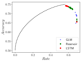
Figure 2: Predictive rate–accuracy curve for the Even Process in Fig. 1, along with empirical predictive accuracies and rates of GLMs, RCs, and LSTMs of various sizes: orders range from $1$-$10$ for GLMs, number of nodes range from $1$-$61$ for RCs, and number of nodes range from $1$-$121$ for LSTMs. Despite the Even Process’ simplicity, there is a noticeable difference between the predictors’ performances and the optimal achievable performance.

First, we analyze the Even Process shown in Fig. 1. The optimal prediction algorithm is easily seen by inspection of Fig. 1. When we determine the machine is in state $A$, we predict a $0$ or a $1$ with equal probability; if it is in state $B$, we predict a $1$. We determine whether or not it is in state $A$ or $B$ by the parity of the number of $1$s since the last $0$. If odd, it is in state $B$; if even, it is in state $A$. The inferred state is easily encoded by the following RNN:

$$h_{t+1}=x_{t}(1-h_{t})~{}.$$ (7)

If $x_{t}$ is $0$, the hidden state of the RNN “resets” to $0$; e.g., state $A$. If $x_{t}=1$, then the hidden state updates by flipping from $0$ to $1$ or vice versa, mimicking the transitions from $A$ to $B$ and back. One can show that a one-node LSTM hidden state $h_{t}$ can, with proper weight choices, mimic the hidden state of Eq. (7). With the correct hidden state inferred, it is straightforward to find $w$ and $w_{0}$ such that Eq. (6) yields optimal (and correct) predictions.

As one might then expect, and as Fig. 2 confirms, LSTMs tend to have rates that are close to the optimal (maximal) rate and predictive accuracies that are only slightly below the optimal predictive accuracy. RCs and GLMs tend to have higher rates and lower predictive accuracies, but they are still within $\sim 13\%$ of optimal. As one might also expect, LSTMs and RCs with additional nodes and GLMs with higher orders (higher $k$) have higher predictive accuracies than LSTMs and RCs with fewer nodes and GLMs with lower orders. But viewed another way, given the simplicity of the stimulus—indeed, given that a one-node LSTM can, in theory, learn the Even Process—the gap from the predictors’ rates and accuracies to the optimal combinations of rate and accuracy is surprising. It is also surprising that none of the three predictors’ rates fall below the maximal optimal rate.

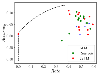
Figure 3: Predictive rate-accuracy curve for the Neven Process (PDFA shown at top), along with empirical predictive accuracies and rates of GLMs, RCs, and LSTMs of various sizes: orders range from $1$-$10$ for GLMs, number of nodes range from $1$-$61$ for RCs, and number of nodes range from $1$-$121$ for LSTMs. Despite Neven Process’ simplicity, there is a noticeable gap between the predictor’s performance and the optimal performance achievable.

Figure 3 introduces a similarly-simple three-state PDFA. If a $1$ is observed after a $0$, we are certain the machine is in state $B$; after state $B$, we know it will transition to state $A$; and then the parity of $0$s following transition to state $A$ tells us if it is in state $A$ (even) or state $B$ (odd). This PDFA is a combination of a Noisy Period-$2$ Process (between states $A$ and $B$) and an Even Process (between states $A$ and $C$).

Given the Neven Process’s simplicity, it is unsurprising that we can concoct an RNN that can infer the internal state. Let $h_{t}=(h_{t,A},h_{t,B},h_{t,C})$ be the hidden state that is $(1,0,0)$ if the internal state is $A$, $(0,1,0)$ if the internal state is $B$, and $(0,0,1)$ if the internal state is $C$. By inspection, we have:

$$h_{t+1,A} =1-h_{t,A}$$

$$h_{t+1,B} =x_{t}h_{t,A}$$

$$h_{t+1,C} =(1-x_{t})h_{t,A}~{}.$$

One can straightforwardly find weights that lead to $p_{LSTM}(x_{t+1}|h_{t})$ accurately reflecting the transmission (emission) probabilities. In other words, in theory a three-node RNN (and an equivalent three-node LSTM) can learn to predict the Neven process optimally.

However, the Neven Process’ simplicity is belied by the gap between the predictors’ accuracy and rate and the predictive rate-accuracy curve. The worst predictive accuracy falls short of the optimal by $\sim 15\%$, and none of the GLMs, RCs, or LSTMs get closer than $\sim 97\%$ to optimal. Furthermore, almost all the rates surpass the maximal optimal predictor rate.

IV-B Comparing GLMs, RCs, and LSTMs

We now analyze the combined results obtained over all minimal PDFAs up to four states using two metrics. (Again, recall that they are $1,338$ unique machine topologies.) To compare across PDFAs, we first normalize the rate and accuracy by the rate and accuracy of the optimal predictor. Then, we find the distance from the predictor’s rate and accuracy to the predictive rate-accuracy curve, which is similar in spirit to the metric of Ref. [42] and to the spirit of Ref. [26]. Note that this metric would have been markedly harder to estimate had we used nondeterministic probabilistic finite automata; that is, those without determinism (unifiliarity) in their transition structure [11].

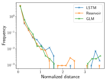
Figure 4: Histogram of normalized distances to the predictive rate-accuracy curve for LSTMs (blue), RCs (orange), and GLMs (green) using $1755$ distinct PDFAs.

Figure 4 showcases a histogram of the normalized distance to the predictive rate-accuracy curve, ignoring PDFAs for which the maximal optimal rate is $0$ nats. The normalized distance for all three predictor types tends to be quite small, but even so, we can see differences in the three predictor types. LSTMs tend to have smaller normalized distances than RCs, and RCs tend to have smaller normalized distances to the predictive rate-accuracy curve than GLMs.

The same trend holds for the percentage difference between the predictive accuracy and the maximal predictive accuracy, which we call the normalized predictive distortion. Trained LSTMs on average have $3.9\%$ predictive distortion; RCs on average have $4.0\%$ predictive distortion; and GLMs on average have $6.5\%$ predictive distortion. When looking only at optimized LSTMs, RCs, and GLMs—meaning that the number of nodes or the order is chosen to minimize normalized predictive distortion—a few PDFAs still have high normalized predictive distortions of $4.6\%$ for LSTMs, $9.7\%$ for RCs, and $27.3\%$ for GLMs. Some LSTMs, RCs, and GLMs reach normalized predictive distortions of as much as $50\%$.

Unsurprisingly, increasing the GLM order and the number of nodes of the RCs and LSTMs tends to increase predictive accuracy and decrease the normalized distance.

Our final aim is to understand the PDFA characteristics that cause them to be harder to predict accurately and/or efficiently. We have two suspects, which are the most natural measures of process “complexity”. This first is the generated process’ entropy rate $h_{\mu}$, the entropy of the next symbol conditioned on all previous symbols, which quantifies the intrinsic randomness of the stimulus. The second is the generated process’ statistical complexity $C_{\mu}$, the entropy of the causal states, which quantifies the intrinsic memory in the stimulus. The more random a stimulus, the harder it would be to predict; imagine having to find the optimal predictor for a biased coin whose bias is quite close to $1/2$. The more memory in a stimulus, the more nodes in a network or the higher the order of the GLM required, it would seem. We performed a multivariate linear regression, trying to use $h_{\mu}$ and $C_{\mu}$ to predict the minimal normalized predictive distortion and minimal normalized distance. We find a small and positive correlation for LSTMs, reservoirs, and GLMs for predicting normalized distance, with an $R^{2}$ of $0.002$, $0.12$, and $0.15$, respectively. We find a larger positive correlation for LSTMs, reservoirs, and GLMs for predicting normalized distortion, with an $R^{2}$ of $0.09$, $0.24$, and $0.24$, respectively. Interestingly, the performance GLMs and RCs is impacted by increased randomness and increased memory in the stimulus, while the LSTMs’ accuracy has little correlation with entropy rate and statistical complexity.

V Conclusion

We have known for a long time that reservoirs and RNNs can reproduce any dynamical system[1, 2, 3], and we have explicit examples of RNNs learning to infer the hidden states of a PDFA when shown the PDFA’s output [4]. We revisited these examples to better understand if the finding of Ref. [4] is typical. How often do RNNs and RCs learn efficient and accurate predictors of PDFAs, especially given that BSI can yield an optimal predictor with orders-of-magnitude less training data?

We conducted a rather comprehensive search, analyzing all $1,388$ randomly-generated PDFAs with four states or less. For each PDFA, we trained GLMs, RCs, and RNNs of varying orders or varying numbers of nodes. Larger orders and larger numbers of nodes led to more accurate and more efficient predictors. On average, the various time series predictors have $\sim 5\%$ predictive distortion. In other words, we are apparently better at classifying MNIST digits than sometimes predicting the output of a simple PDFA. And again, existing algorithms [13] can optimally predict the output of the PDFAs considered here with orders-of-magnitude less training data. These findings lead us to conclude that algorithms that explicitly focus on inference of causal states [14, 13, 15, 16] have a place in the currently RNN-dominated field of time series prediction.

References

- [1] W. Maass, T. Natschläger, and H. Markram, “Real-time computing without stable states: A new framework for neural computation based on perturbations,” Neural Comp., vol. 14, no. 11, pp. 2531–2560, 2002.
- [2] L. Grigoryeva and J.-P. Ortega, “Echo state networks are universal,” Neural Networks, vol. 108, pp. 495–508, 2018.
- [3] K. Doya, “Universality of fully connected recurrent neural networks,” Dept. of Biology, UCSD, Tech. Rep, 1993.
- [4] A. Cleeremans, D. Servan-Schreiber, and J. L. McClelland, “Finite state automata and simple recurrent networks,” Neural Comp., vol. 1, no. 3, pp. 372–381, 1989.
- [5] B. G. Horne and D. R. Hush, “Bounds on the complexity of recurrent neural network implementations of finite state machines,” in Adv. Neural Info. Proc. Sys., 1994, pp. 359–366.
- [6] J. Schmidhuber and S. Hochreiter, “Long short-term memory,” Neural Comput, vol. 9, no. 8, pp. 1735–1780, 1997.
- [7] J. Collins, J. Sohl-Dickstein, and D. Sussillo, “Capacity and trainability in recurrent neural networks,” arXiv:1611.09913.
- [8] C. R. Shalizi and J. P. Crutchfield, “Computational mechanics: Pattern and prediction, structure and simplicity,” J. Stat. Phys., vol. 104, pp. 817–879, 2001.
- [9] W. Bialek, I. Nemenman, and N. Tishby, Neural Comp., vol. 13, pp. 2409–2463, 2001.
- [10] J. P. Crutchfield and D. P. Feldman, “Regularities unseen, randomness observed: Levels of entropy convergence,” CHAOS, vol. 13, no. 1, pp. 25–54, 2003.
- [11] S. Marzen and J. P. Crutchfield, “Predictive rate-distortion for infinite-order Markov processes,” J. Stat. Phys., vol. 163, no. 6, pp. 1312–1338, 2014.
- [12] J. A. Nelder and R. W. Wedderburn, “Generalized linear models,” J. Roy. Stat. Stoc. A, vol. 135, no. 3, pp. 370–384, 1972.
- [13] C. C. Strelioff and J. P. Crutchfield, “Bayesian structural inference for hidden processes,” Phys. Rev. E, vol. 89, p. 042119, 2014.
- [14] J. P. Crutchfield and K. Young, “Inferring statistical complexity,” Phys. Rev. Let., vol. 63, pp. 105–108, 1989.
- [15] D. Pfau, N. Bartlett, and F. Wood, “Probabilistic deterministic infinite automata,” in Adv. Neural Info. Proc. Sys., 2010, pp. 1930–1938.
- [16] S. Still, “Information bottleneck approach to predictive inference,” Entropy, vol. 16, no. 2, pp. 968–989, 2014.
- [17] M. L. Littman and R. S. Sutton, “Predictive representations of state,” in Advances in neural information processing systems, 2002, pp. 1555–1561.
- [18] W. Schultz, P. Dayan, and P. R. Montague, “A neural substrate of prediction and reward,” Science, vol. 275, no. 5306, pp. 1593–1599, 1997.
- [19] P. R. Montague, P. Dayan, and T. J. Sejnowski, “A framework for mesencephalic dopamine systems based on predictive Hebbian learning,” J. Neurosci., vol. 16, no. 5, pp. 1936–1947, 1996.
- [20] R. P. Rao and D. H. Ballard, “Predictive coding in the visual cortex: a functional interpretation of some extra-classical receptive-field effects,” Nature neuroscience, vol. 2, no. 1, p. 79, 1999.
- [21] T. Berger, Rate Distortion Theory. New York: Prentice-Hall, 1971.
- [22] S. Still, J. P. Crutchfield, and C. J. Ellison, “Optimal causal inference: Estimating stored information and approximating causal architecture,” Chaos: An Interdisciplinary Journal of Nonlinear Science, vol. 20, no. 3, p. 037111, 2010.
- [23] N. Tishby, F. C. Pereira, and W. Bialek, “The information bottleneck method,” physics/0004057.
- [24] F. Creutzig and H. Sprekeler, “Predictive coding and the slowness principle: An information-theoretic approach,” Neural Computation, vol. 20, no. 4, pp. 1026–1041, 2008.
- [25] F. Creutzig, A. Globerson, and N. Tishby, Phys. Rev. E, vol. 79, no. 4, p. 041925, 2009.
- [26] S. E. Palmer, O. Marre, M. J. Berry, and W. Bialek, “Predictive information in a sensory population,” Proc. Natl. Acad. Sci. USA, vol. 112, no. 22, pp. 6908–6913, 2015.
- [27] J. E. Hopcroft and J. D. Ullman, Introduction to Automata Theory, Languages, and Computation. Reading: Addison-Wesley, 1979.
- [28] R. B. Ash, Information Theory. New York: John Wiley and Sons, 1965.
- [29] R. G. James, J. R. Mahoney, C. J. Ellison, and J. P. Crutchfield, “Many roads to synchrony: Natural time scales and their algorithms,” Phys. Rev. E, vol. 89, p. 042135, 2014.
- [30] W. Löhr, “Models of discrete-time stochastic processes and associated complexity measures,” Ph.D. dissertation, University of Leipzig, May 2009.
- [31] C. R. Shalizi, K. L. Shalizi, and J. P. Crutchfield, “Pattern discovery in time series, part i: Theory, algorithm, analysis, and convergence,” Journal of Machine Learning Research, 2002.
- [32] I. Csiszár, “On the computation of rate-distortion functions (corresp.),” IEEE Transactions on Information Theory, vol. 20, no. 1, pp. 122–124, 1974.
- [33] B. D. Johnson, J. P. Crutchfield, C. J. Ellison, and C. S. McTague, “Enumerating finitary processes,” arxiv.org:1011.0036.
- [34] J. P. Crutchfield and K. Young, “Computation at the onset of chaos,” in Entropy, Complexity, and the Physics of Information, ser. SFI Studies in the Sciences of Complexity, W. Zurek, Ed., vol. VIII. Reading, Massachusetts: Addison-Wesley, 1990, pp. 223 – 269.
- [35] N. H. Packard, “Adaptation toward the edge of chaos,” in Dynamic Patterns in Complex Systems, A. J. M. J. A. S. Kelso and M. F. Shlesinger, Eds. Singapore: World Scientific, 1988, pp. 293 – 301.
- [36] M. Mitchell, J. P. Crutchfield, and P. Hraber, “Dynamics, computation, and the “edge of chaos”: A re-examination,” in Complexity: Metaphors, Models, and Reality, ser. Santa Fe Institute Studies in the Sciences of Complexity, G. Cowan, D. Pines, and D. Melzner, Eds., vol. XIX. Reading, MA: Addison-Wesley, 1994, pp. 497 – 513.
- [37] M. Mitchell, P. Hraber, and J. P. Crutchfield, “Revisiting the edge of chaos: Evolving cellular automata to perform computations,” Complex Systems, vol. 7, pp. 89 – 130, 1993.
- [38] N. Bertschinger and T. Natschläger, “Real-time computation at the edge of chaos in recurrent neural networks,” Neural Comp., vol. 16, no. 7, pp. 1413–1436, 2004.
- [39] J. Boedecker, O. Obst, J. T. Lizier, N. M. Mayer, and M. Asada, “Information processing in echo state networks at the edge of chaos,” Theory in Biosciences, vol. 131, no. 3, pp. 205–213, 2012.
- [40] S. Hochreiter, “The vanishing gradient problem during learning recurrent neural nets and problem solutions,” International Journal of Uncertainty, Fuzziness and Knowledge-Based Systems, vol. 6, no. 02, pp. 107–116, 1998.
- [41] D. P. Kingma and J. Ba, “Adam: A method for stochastic optimization,” arXiv:1412.6980.
- [42] N. Zaslavsky, C. Kemp, T. Regier, and N. Tishby, “Efficient compression in color naming and its evolution,” Proc. Natl. Acad. Sci. USA, vol. 115, no. 31, pp. 7937–7942, 2018.