Community Detection in Multiplex Networks

Abstract

A multiplex network models different modes of interaction among same-type entities. In this article we provide a taxonomy of community detection algorithms in multiplex networks. We characterize the different algorithms based on various properties and we discuss the type of communities detected by each method. We then provide an extensive experimental evaluation of the reviewed methods to answer three main questions: to what extent the evaluated methods are able to detect ground-truth communities, to what extent different methods produce similar community structures and to what extent the evaluated methods are scalable. One goal of this survey is to help scholars and practitioners to choose the right methods for the data and the task at hand, while also emphasizing when such choice is problematic.

1 Introduction

Multiplex network analysis has emerged as a promising approach to investigate complex systems. A multiplex network is a model used to represent multiple modes of interaction or different types of relationships among entities of the same type (e.g. people). This model has been used to study a large variety of systems across disciplines, ranging from living organisms and human societies to transportation systems and critical infrastructures. For example, a description of the full protein-protein interactome involves, for some organisms, up to seven distinct modes of interaction among thousands of protein molecules [15]. Another example is in air transportation systems when modeling the connections between airports through direct flights; here, the different commercial airlines can be seen as different modes of connection among airports [11].

Figure 1 shows a typical layered representation of a multiplex network, where each layer corresponds to a type of interaction and nodes (also called vertices) in different layers can be associated to the same actor, e.g. the same person or the same airport. Here, we adopt the term actor from the field of social network analysis, where multiplex networks have been first applied, and the term layer from recent generalizations of the original multiplex model [10, 38, 31, 16].

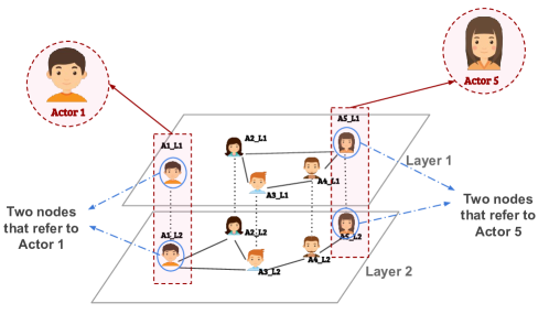
Figure 1: An example of a multiplex network with two types of interaction among five actors. This is represented as five nodes replicated in two layers. The two nodes representing the same actor (e.g. the same person) are linked by a dotted line

A core task in network analysis is to identify and understand communities, also known as clusters or cohesive groups; that is, to explain why groups of entities (actors) belong together based on the explicit ties among them and/or the implicit ties induced by some similarity measures given some attributes of these entities. Since members of a community tend to share common properties, revealing the community structure in a network can provide a better understanding of the overall functioning of the network.

Unfortunately, community detection methods for simple graphs are not sufficient to deal with the complexity of the multiplex model, for three main reasons. First, without allowing the analysis of subsets of the layers some communities may become hidden by edges in irrelevant layers. This is a common problem also in traditional multivariate data analysis, where several preprocessing methods have been developed to remove irrelevant information and algorithms have been extended to explore subsets of the data dimensions, as done by subspace clustering methods. Second, algorithms not explicitly representing the different layers cannot differentiate between different types of multiplex communities, e.g., those present on a single layer and those made of specific combinations of layers. Third, without a concept of layer it is not possible to include the same actor in different communities depending on the layer where the actor is active. In other words, community detection methods for simple graphs cannot conceptually represent (and thus discover) some types of communities that can only be defined on multilayer networks, although this does not imply that non-multilayer methods will always be outperformed by multilayer algorithms.

To address the above limitations, several community detection algorithms for multiplex networks have been recently proposed, based on different definitions of community and different computational approaches. Recent works have provided a partial overview of existing algorithms. [29] proposed some criteria to compare multi-layered community detection algorithms, but without any experimental evaluation. Similarly, [6] highlighted the conceptual differences among different clustering methods over attributed graphs, including edge-labeled graphs that can be used to represent multiplex networks, but only provided a taxonomy of the different algorithms without any experimental analysis. [36] instead performed a pairwise comparison of the different clusterings produced by some existing algorithms. The work by [24] provides a more general overview on multilayer networks (which include multiplex networks), but without comprehensive experiments.

This article provides a systematic review and experimental comparison of existing methods, with the aim of simplifying the choice and the setup of the most appropriate algorithm for the task at hand. We test the accuracy of the different methods with respect to some given ground truth on both synthetic and real networks and we study their scalability in terms of the size of the network, both vertically (number of layers) and horizontally (number of actors). At the same time, we highlight weaknesses and strengths of specific methods and of the current state-of-the-art as a whole, showing how even the most sophisticated methods fail to identify some types of communities.

The focus of this survey is on algorithms explicitly designed to discover communities in multiplex networks through the analysis of the network structure. Several community detection algorithms have been proposed to deal with models related to but not compatible with the multiplex model, such as Heterogeneous Information Networks [49, 50, 59, 51] and bipartite networks [2, 20], and are not included in our article. Since we focus on network structure, graph clustering on attributed networks [5, 47, 48, 56, 58, 45, 34] is also not included in our analysis. For a survey on attributed graph clustering we refer the reader to [6].

The rest of this work is organized as follows. Section 2 provides some basic definitions used throughout the article. In Section 3 we introduce a taxonomy of existing multiplex community detection methods. Section 4 provides a theoretical comparison of the reviewed algorithms, while Section 5 presents the experimental settings and the evaluation datasets used in our experiments. The results of the experimental analysis are given in Section 6. We summarize our main findings and indicate usage guidelines emerged from our experiments in Section 7.

2 Multiplex networks and communities

A multiplex network is a special case of a multilayer network. A multilayer network is defined as a tuple $(A,L,V,E)$, where $A$ is a set of actors, $L$ is a set of layers, and $(V,E)$ is a graph on $V\subseteq A\times L$. Notice that this definition does not require all the actors to be present in all the layers, and allows actors to be present in some layers without having any neighbor on those layers.

In multiplex networks $E$ is restricted to intra-layer edges, that is, an edge $((v_{1},l_{1}),(v_{2},l_{2}))$ is allowed only if $l_{1}=l_{2}$. In the following we use $a$, $l$, $v$, and $e$ to refer to the cardinality of, respectively, $A$, $L$, $V$, and $E$. We use the terms vertex or node to indicate the elements of $V$, that is, actors inside a layer.

The most common output of a community detection algorithm for multiplex networks is a set of communities $\mathcal{C}$ = $\{C_{1},C_{2},\dots,C_{k}\}$ such that each community contains a non-empty subset of $V$. $\mathcal{C}$ is a representation of the community structure of the network. Sometimes the term cluster is also used as a synonym of community, although the term community can be interpreted more broadly to also refer to the subgraph induced by its nodes, or even more broadly to indicate the real-world concept it represents, e.g., a group of people with shared norms, values or objectives in a social network. A few community detection methods discover clusters of edges instead of clusters of nodes or actors. Keeping the above considerations in mind, the term clustering is also used to refer to the set of all communities. Figure 2 illustrates different possible types of clusterings on a multiplex network.

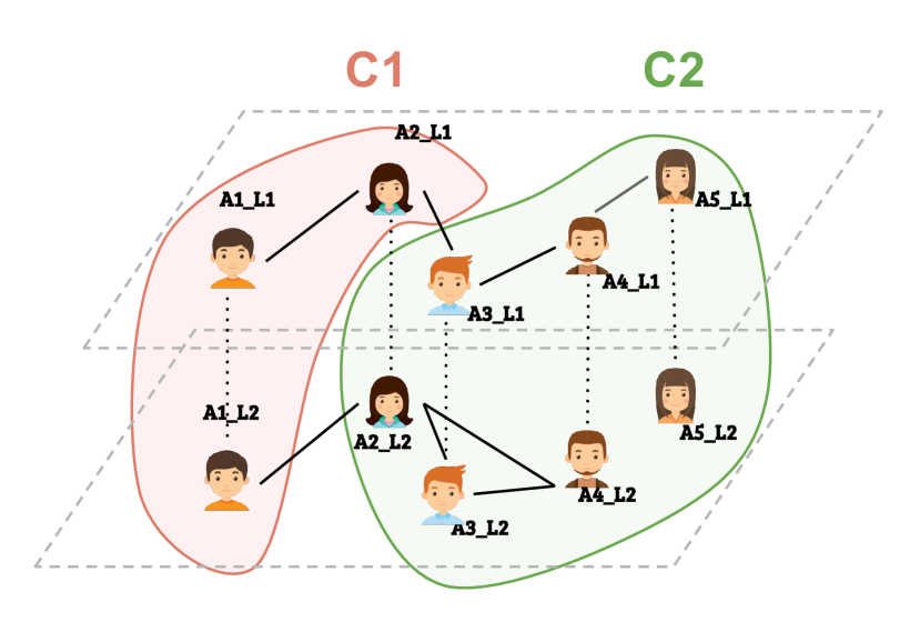
(a) Total

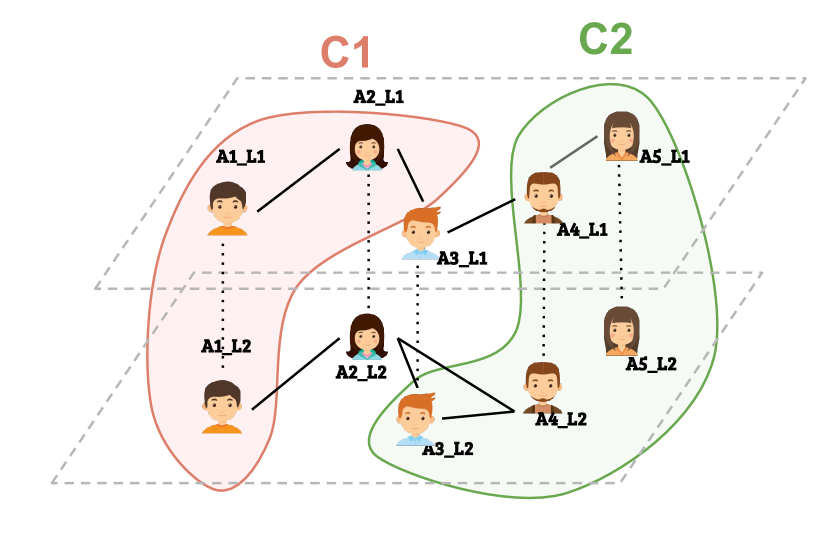
(b) Partial

(c) Node-overlapping

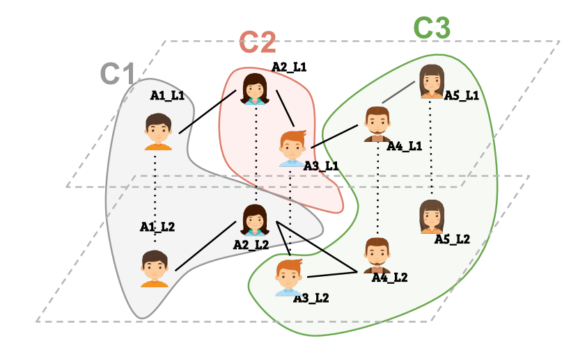
(d) Node-disjoint

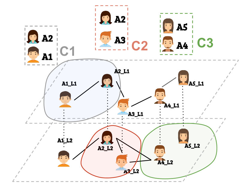
(e) Actor-overlapping

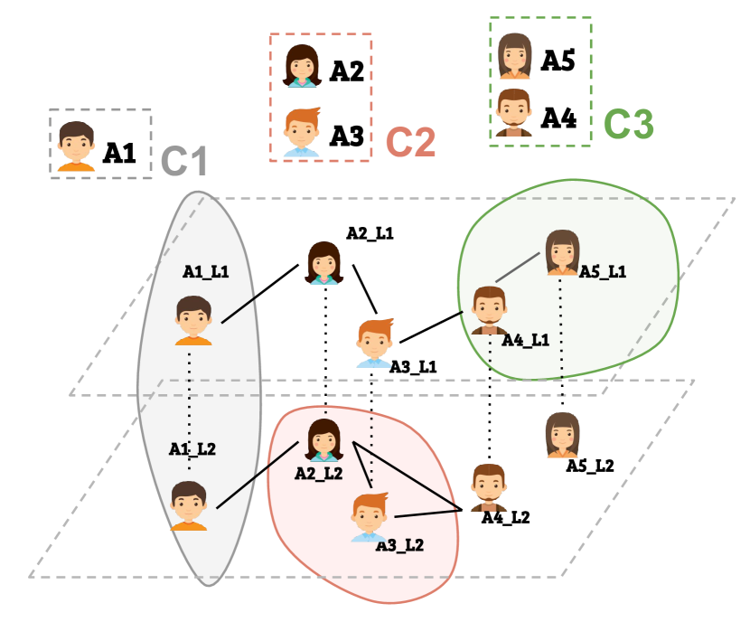
(f) Actor-disjoint

Figure 2: Different types of clustering on a multiplex network. In (c) the two overlapping nodes are A4_L1 and A3_L2. In (e) A2 is the overlapping actor

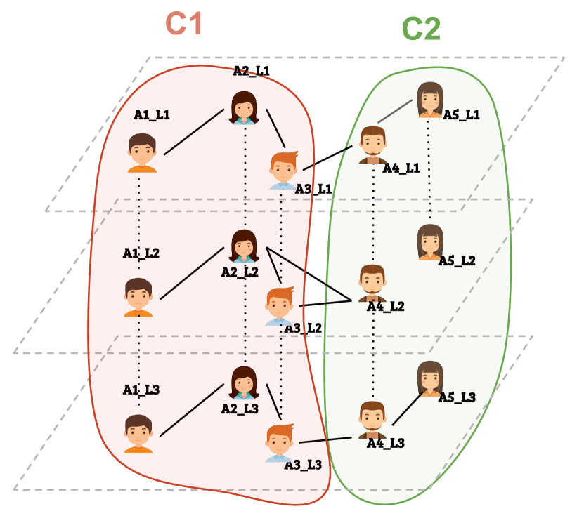
(a) Pillar communities

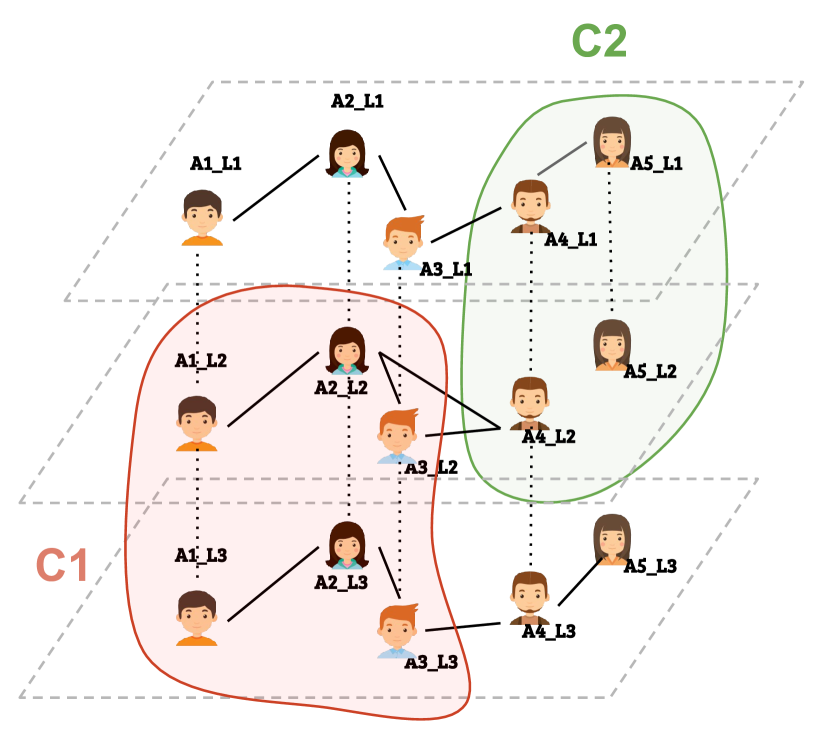
(b) Semi-pillar communities

Figure 3: Pillar and semi-pillar multiplex community structures

A clustering $\mathcal{C}$ is total if every node in $V$ belongs to at least one community, and it is partial otherwise. We also call a clustering node-overlapping if there is at least a node that belongs to more than one cluster, otherwise the clustering is called node-disjoint. Analogously, if there is at least an actor belonging to more than one cluster we call the clustering actor-overlapping, otherwise it is called actor-disjoint. Notice that a node-overlapping clustering is also actor-overlapping, while an actor-overlapping clustering may or may not be node-overlapping.

Finally, a multiplex community is called semi-pillar on layers $L^{\prime}\subset L$ if for each actor $a\in A$ in the community all nodes in $\{(a,l)\in V:l\in L^{\prime}\}$ are included in the community. When $L^{\prime}=L$ we talk of a pillar community (Figure 3). Please notice that two pillar communities are either disjoint or both actor- and node-overlapping.

3 A taxonomy of the reviewed algorithms

In this section we provide a taxonomy of multiplex community detection methods with three levels of classification. The top-level distinction is between global or local methods, respectively discovering all communities in the input network or generating a single community around one or more seed nodes. The results of these two types of algorithms are not directly comparable without arbitrary choices in the selection of seed nodes, so we treat them in separate sections in our experimental evaluation. The second level regards the way in which the algorithms handle the presence of multiple layers: reducing them to a single layer (flattening), processing each layer independently (e.g., performing single-layer community detection) to then merge the results of the processing, or considering all the layers at the same time. The last level of the taxonomy groups the algorithms based on more specific approaches, such as optimizing an objective function, considering the behavior of a random walker or identifying dense subgraphs. Figure 4 and Table 4 show an overview of the related methods. Please notice that Section 4, describing some theoretical properties of the algorithms such as whether they are deterministic or not, can also be used to differentiate between different types of algorithms.

Figure 4: A taxonomy of multiplex community detection algorithms

Table 1: Multiplex community detection algorithms covered in this survey

Algorithm	Notation	Reference
Non-Weighted Flattening	NWF	[3]
Weighted Flattening (Edge Count)	WF_EC	[3]
Weighted Flattening (Neighbourhood)	WF_N	[3]
Weighted Flattening (Differential)	WF_Diff	[30]
Frequent pattern mining-based community discovery	ABACUS	[4]
Ensemble-based Multi-layer Community Detection	EMCD	[52]
Principal Modularity Maximization	PMM	[54, 55]
Subspace Analysis on Grassmann Manifolds	SCML	[17]
Cross-Layer Edge Clustering Coefficient (based on)	CLECC	[9]
Multi Layer Clique Percolation Method	ML-CPM	[1]
Locally Adaptive Random Transitions	LART	[32]
Modular Flows on Multilayer Networks	Infomap	[14, 18]
Generalized Louvain	GLouvain	[41, 28]
Fast algorithm for comm. detection based on multiplex net. modularity	FCDMNN	[57]
Multilink community detection	MLink	[39]
Multi-Layer Many-objective OPtimization algorithm	MLMaOP	[44]
Multilevel memetic algorithm for composite community detection	MNCD	[37]
Multi Dimensional Label Propagation	MDLPA	[7]
Andersen-Chung-Lang cut	ACLcut	[27]
Multilayer local community detection	ML-LCD	[26]

3.1 Global methods

Global methods are designed to discover all possible communities in a network, thus requiring knowledge of the whole network structure. As it happens for many multiplex data analysis methods [16], global community detection algorithms can also be grouped into three typical main classes, described in the following.

3.1.1 Flattening

The first approach consists in simplifying the multiplex network into a graph by merging its layers, using a so-called flattening algorithm, then applying a traditional community detection algorithm. This process is illustrated in Figure 5.

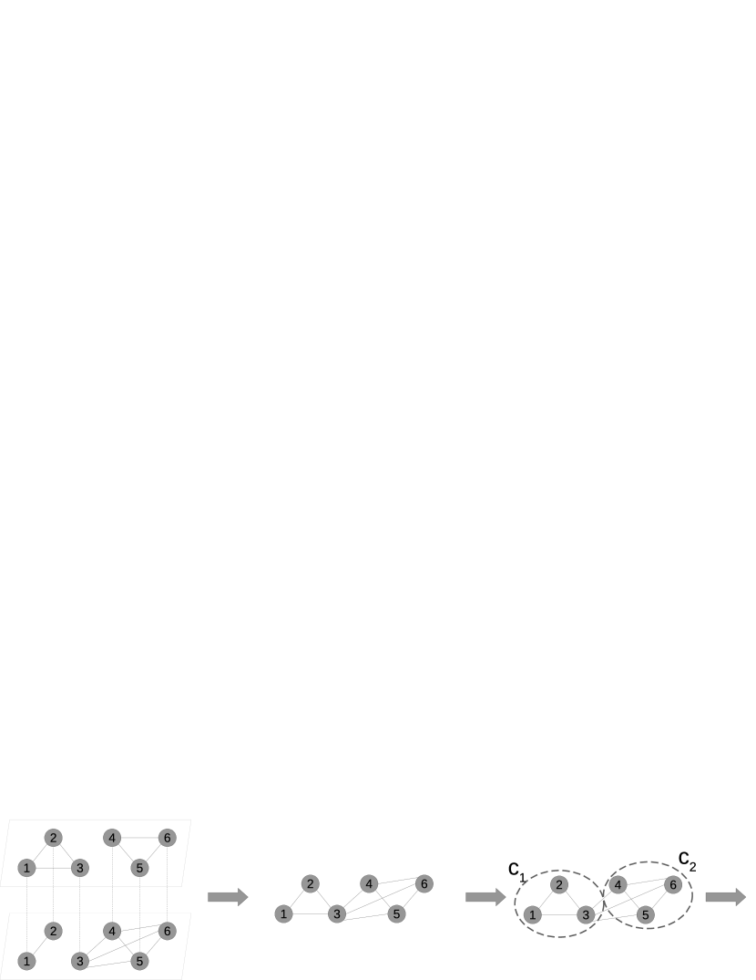
Figure 5: The general process used by flattening methods: a single-layer network is first constructed merging edges from the different layers, then a traditional community detection algorithm is applied to the flattened network, and its result can be used to induce communities on the original network

The algorithms belonging to this class are defined by the flattening method and by the single-layer community detection algorithm applied to the flattened network. The simplest flattening method consists in creating an unweighted graph where two nodes are adjacent if their corresponding actors are adjacent on any of the input layers [3]. The advantage of this approach is that the resulting graph is easier to handle, because there are more clustering algorithms for simple graphs than for weighted graphs and weights often imply an additional level of complexity, e.g., deciding a threshold above which weighted edges should be considered. A potential disadvantage is that an unweighted flattening is more susceptible to noise.

Weighted flattenings reflect some structural properties of the original multiplex network in the form of weights assigned to the output edges [3, 30]. In theory these methods are less susceptible to noise, but the resulting communities may be biased towards edges appearing on several layers, and the results can be more difficult to interpret because of the weights.

In general, the algorithms in this class are only able to identify pillar communities, and some communities may emerge because of edges spread on different layers that would not constitute a community on any individual layer, because of the flattening process.

3.1.2 Layer by layer

While the methods in the previous class merge the layers and then apply traditional community detection algorithms, layer-by-layer methods first process each layer (e.g., applying traditional community detection algorithms), then merge the results of the processing. This is illustrated in Figure 6.

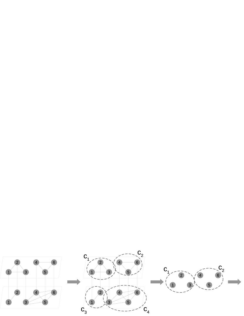
Figure 6: The general process used by layer-by-layer methods: communities are identified in each layer, the information obtained from each layer is used to cluster the actors, and this clustering can be used to induce communities on the original network

As a consequence of the layer-by-layer community detection step, these methods include actors in the same community only when they are part of the same community in at least one layer. Also, due to the merging of layer-specific communities, these methods can in principle only identify pillar communities.

We have identified three types of layer-by-layer approaches in the literature. The pattern mining approach exploits association rule mining methods, which are among the main data mining tasks used to find objects that frequently co-occur together in different transactions. (A typical example of transaction is the basket of products bought together by a customer at a supermarket.) ABACUS considers each single-layer community as a transaction, so that the final communities contain actors that are part of the same community in at least a minimum number of layers [4].

The second way to merge the result of single-layer community detection methods is based on a notion of consensus: given a set (or ensemble) of community structure solutions from the individual layers, the goal is to find a single, meaningful solution that is representative of the input ensemble, by optimizing an objective function that is designed to aggregate information from the individual solutions in the ensemble. While early approaches such as the one in [33] are limited to use a clustering ensemble method as a black-box tool for combining multiple clustering solutions from a single-layer network, the first well-principled formulation of the ensemble-based multilayer community detection (EMCD) problem, provided in [52], does not limit aggregation at node membership level, but rather it accounts for intra-community and inter-community connectivity. The consensus solution discovered by EMCD is the one with maximum multilayer modularity from a search space of candidates delimited by topological upper-bound and lower-bound solutions, respectively, of the input multilayer network.

Finally, some methods in the literature process the layer-specific adjacency matrices, or derived matrices, and extend spectral-clustering for simple graphs by exploiting the relationship between the eigenvectors and eigenvalues in the constructed matrices and the presence of clusters in the corresponding graphs. As an example, the principal modularity maximization (PMM) method [54] extracts structural features from the various layers, then concatenates the features and performs PCA to select the top eigenvectors. Using these eigenvectors, a low-dimensional embedding is computed to capture the principal patterns across the layers, finally a simple $k$-means is applied to assign nodes to communities. Further details on this class of approaches can be found in [53].

3.1.3 Multilayer

The third class of algorithms operates directly on the multiplex network model, as shown in Figure 7. As an example, a method belonging to this class based on a random walker would allow the walker to switch from one layer to the other.

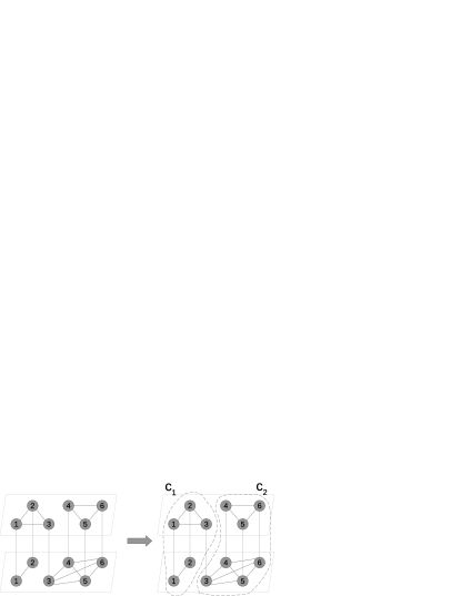
Figure 7: Multilayer methods discover communities directly on the multiplex data

Various approaches originally developed for simple graphs have been extended to the multilayer case. Density-based methods first identify dense regions of the network, then include adjacent regions in the same community. A popular method for simple graphs is clique percolation, where dense regions correspond to cliques and adjacency consists in having common nodes. The multilayer clique percolation method (ML-CPM) extends this process by looking for cliques spanning multiple layers, and redefining adjacency so that both common nodes and common layers are required [1]. CLECC uses a different but related approach, identifying sparse locations of the network having a low cross-layer clustering coefficient [9]. The higher the proportion of common neighbors across all layers (or any number of layers provided as input), the higher the cross-layer clustering coefficient.

Methods based on random walks consider that an entity randomly following the edges in a network would tend to get trapped inside communities, because of the higher edge density between nodes inside the same community, less frequently moving from one community to the other. LART [32] and Infomap [14] are both based on this consideration, with Infomap using a shortest information coding approach to identify the corresponding communities.

Several of the reviewed algorithms in the multilayer class use an objective function that, given an assignment of the nodes to communities, returns a higher value when there are more edges inside communities and less edges across communities. Once the objective function has been defined, then different optimization methods can be used to identify a community assignment corresponding to a high value of the function. Generalized Louvain (GLouvain) [41, 28], the best-known method in this class, uses an extended version of modularity, and has been analyzed in more detail in [21]. While GLouvain has become the most popular modularity-based method for multiplex networks, it is worth mentioning the alternative approach used by [44], aimed at obtaining a high modularity in each individual layer instead of a global extended definition of modularity. This class also includes a method returning a different type of communities with respect to the ones generated by the other algorithms, where edges are grouped instead of actors and nodes [39].

Finally, the multilayer class includes an algorithm based on label propagation [7]. A traditional label propagation method would start assigning a different label to each node, then having each node replace its label with one that is frequent among its neighbors, until some stopping condition is satisfied. The multilayer version of this approach follows the same idea, weighting the contribution of each neighbor based on their similarity with the node on the different layers. For example, two nodes being adjacent on all layers and having the same neighbors on all layers would have a higher probability of getting the same label.

3.2 Local methods

Local methods (also known as node-centric) are query-dependent, i.e., they are designed to discover the community around a set of input query nodes. Please notice that the term local has also been used with other meanings in the literature, for methods finding global community structures using only neighborhood information when processing vertices in the graph. At the time of writing, we recognize the availability of two methods able to discover multiplex local communities: ML-LCD [26] and ACLcut [27]. ML-LCD searches for the local community associated to a seed actor without having a complete knowledge of the network graph, through an incremental exploration of the neighborhood of the query actor, according to the optimization of a criterion function based on the internal and external connectivity of the local community. ACLcut exploits the solution of a personalized PageRank approximated for an input seed-set (i.e., a set of query actors) in order to find the local communities, using a sweep cut method to sample local communities based on the lowest conductance values. Both methods operate directly on the multiplex network model, so that the Local branch of our hierarchy only includes the Multilayer class. Nevertheless (even if, to the best of our knowledge, there are no such examples in literature) it is in theory possible to easily design multiplex local community detection methods that operate through flattening or layer-by-layer schemes, by exploiting existing single-layer local community detection methods such as LCD [12] and Lemon [35].

3.3 Selection of algorithms

In the following sections we will provide a detailed comparative analysis of a large subset of the algorithms in our taxonomy. We include at least one representative method for each leaf in the taxonomy. In those cases where different well-known methods inside the same leaf show significant differences, either theoretically or experimentally, we have also included them, as detailed in the following.

We only focus on a selection of the flattening methods, with one representative for each class (unweighted and weighted), because of the small variation between the different approaches and because the features and performance of these algorithms are determined more by the single-layer approach used to implement them than by the way in which weights are assigned. While the main interest of this article is on multilayer-specific methods, we still considered it important to test some flattening methods in detail, because as we will see in our comparative analysis these simpler approaches can still produce good and sometimes better results than more sophisticated methods.

We include all the methods from the layer-by-layer class (ABACUS, EMCD, PMM and SCML), because they are representative of different ways to merge the results of the single-layer algorithms. PMM has been first published in conference proceedings [54] and then abstracted and extended in a journal article [55]. We use the conference version, because the code for the journal version is not available.

From the multilayer class we include at least one representative method for each sub-class. Among the modularity-opimization methods we have selected GLouvain because it is the best-known optimization algorithm as witnessed by its large number of citations. MLink has only been included in the scalability analysis because it produces link communities that are not directly comparable with the ones produced by other methods.

We also include all the local methods (ACLcut and ML-LCD), because they use significantly different approaches.

4 Theoretical analysis

In this section we present some theoretical properties of the reviewed algorithms. We describe the types of community structures that can be returned by each algorithm, we indicate some features of the algorithms themselves such as whether they are deterministic, and we discuss parameter setting and computational complexity.

These properties should be considered in combination with the results of our experimental evaluation. For example, the fact that in theory an algorithm is able to produce some types of multiplex communities does not imply that these types of communities will be found in practice. Nonetheless, knowing that some algorithms are not able to return some types of communities or that their execution time grows exponentially with respect to the number of layers can be useful to choose which algorithms to use in specific situations.

4.1 Types of community structures

In Section 2 we have described different properties of multiplex community structures. Table 2 indicates which ones are associated to each reviewed algorithm. In particular,

• if the algorithm can generate Non-Pillar Communities;

• if it can generate Actor-Overlapping community structures;

• if it can generate Node-Overlapping community structures;

• if it can generate Partial community structures.

An algorithm not satisfying these properties (i.e., those with an ‘$\times$’ in the table) would, respectively, only be able to produce pillars, only partition the actors and nodes, and force all nodes to belong to at least one community. Notice that this can be perfectly fine in some cases, so satisfying or not the properties above does not mean that the algorithm is worse or better. These properties should only be used as an indication about the appropriateness of the algorithm for specific scenarios.

Table 2: Types of clustering produced by the reviewed methods and algorithmic properties. The second column recalls the class of the algorithm (G-Flat: global flattening, G-LBL: global layer by layer, G-ML: global multilayer, L-ML: local multilayer). Columns NPC (Non-Pillar), AO (Actor-Overlapping), NO (Node-Overlapping) and Pa (Partial) indicate if the algorithm can (✓) or cannot ($\times$) produce that type of community structure. Columns LR (Layer Relevance), Det (Deterministic), AK (Automated selection of the number of communities) and SS (Subgraph Structure) refer to the functioning of the algorithm. (*) indicates that the answer depends on the single-layer clustering algorithm used by the method. (-) indicates that the property is not relevant for the algorithm. The last column indicates the time complexity of the method if studied in the original paper or easily derivable from the algorithm: $a$: number of actors, $e$: number of edges, $l$: number of layers, $c$: number of communities, ARM: cost to compute closed association rules, $|C|$: size of local community, $d$: maximum node degree, $\delta$: complexity of the single-layer community detection algorithm used as a sub-procedure, $\Phi$: parameter depending on the used subprocedure (see Section 4.4).

Algorithm	Category	NPC	AO	NO	Pa	LR	Det	AK	SS	Compl
NWF	G-Flat	$\times$	*	*	*	$\times$	*	*	*	$\mathcal{O}(e+\delta)$
WFEC	G-Flat	$\times$	*	*	*	$\times$	*	*	*	$\mathcal{O}(e+\delta)$
ABACUS	G-LBL	$\times$	✓	✓	✓	$\times$	*	✓	✓	$\mathcal{O}(l\delta)$ + ARM
EMCD	G-LBL	$\times$	$\times$	$\times$	$\times$	✓	*	✓	✓	$\mathcal{O}(l\delta)+\mathcal{O}(i(e+lc))$
PMM	G-LBL	$\times$	$\times$	$\times$	$\times$	$\times$	$\times$	$\times$	$\times$	–
SCML	G-LBL	$\times$	$\times$	$\times$	$\times$	$\times$	$\times$	$\times$	$\times$	–
ML-CPM	G-ML	✓	✓	✓	✓	$\times$	✓	✓	✓	$\geq\mathcal{O}(l3^{\frac{a}{3}})$
Infomap	G-ML	✓	✓	✓	✓	✓	$\times$	✓	✓	–
LART	G-ML	✓	✓	$\times$	$\times$	✓	$\times$	✓	✓	–
GLouvain	G-ML	✓	✓	$\times$	$\times$	✓	$\times$	✓	✓	–
MDLPA	G-ML	✓	✓	$\times$	$\times$	✓	$\times$	✓	✓	$\mathcal{O}(ea+e2^{l}+ei)$
ML-LCD	L-ML	$\times$	-	-	-	✓	✓	-	✓	$\mathcal{O}(|C|^{2}d\Phi)$
ACLcut	L-ML	✓	-	-	-	$\times$	$\times$	-	✓	–

The following are some considerations summarized in Table 2:

• For all flattening methods, the type of the resulting community structure (Overlapping/Disjoint and Total/Partial) depends on the single-layer algorithm used after flattening. The choice of the single-layer algorithm can then be made depending on the wanted result.

• All flattening methods produce pillar communities, because the actors on different layers are reduced to a single node in the flattened graph.

• All multilayer methods can produce non-pillar communities in theory, although our experimental evaluation shows that pillar communities are often returned by some of these methods.

• Pillar actor-overlapping communities are always node-overlapping, by definition.

• Non-pillar actor-overlapping communities may be or not node-overlapping.

4.2 Algorithmic properties

In their survey work, [29] discussed a classification framework based on a set of desired properties for multilayer community detection methods. These properties are: multiple layer applicability, consideration of each layer’s importance, flexible layer participation (i.e., every community can have a different coverage of the layers’ structure), no-layer-locality assumption (e.g., independence from initialization steps biased by a particular layer), independence from the order of layers, algorithm insensitivity, and overlapping layers (e.g., two or more communities can share substructures over different layers).

We observe that the first of the properties listed above (multiple layer applicability) is satisfied by all methods we reviewed, therefore we do not elaborate on this further. By contrast, the second property (consideration of each layer’s importance) is also included in our list and further elaborated, as detailed below (Layer Relevance). We collapse the properties about independence from the order in which nodes and layers are examined into a single property, also including stochastic behaviors such as in the case of random walkers (Determinism). As we focus on multiplex networks, we do not treat the case where layers are ordered. The insensitivity property (i.e., independence or robustness against main tunable input parameters) is instead replaced by a more specific property on whether the number of communities is automatically derived (Auto-detection), and a more general discussion about how to set additional parameters. The last property we consider (Subgraph Structure) was not discussed in previous surveys.

In light of the above considerations we define the following properties, indicated in Table 2.

• Layer relevance. Some methods take into consideration each layer’s importance, also called relevance in some of the reviewed works, in order to control their contribution to the computation of the multiplex community structure. Layer relevance is either learned based on the layer characteristics, or it can be an input of the algorithm based on a-priori knowledge (e.g., user preferences).

• Determinism. This refers to whether a method has a deterministic behavior, e.g., its output is independent from the order of examination of the nodes and/or layers.

• Auto-detection of the number of communities. Some methods expect the number of communities to be decided ahead of time while other methods can automatically define the number of communities.

• Subgraph structure. The primary product of all the reviewed methods are the cluster memberships of nodes. However, some methods also tell us something about the multilayer subgraph structures underlying each community, that is, we can get more information about which edges contributed to the discovery of each community.

Different algorithms tune layer relevance (LR) in different ways. The only algorithm allowing to specify weights as input parameters is GLouvain, through the parameter omega ($\omega$) that gives more or less importance to the fact that the same actor is included in the same community in different layers. However, these weights are assigned to pairs of actors in different layers, not to individual layers, and in practice $\omega$ is set to a single value for the whole network. In EMCD, the importance of the various layers may be considered by differently setting the resolution parameter in the multilayer modularity. Both LART and MDLPA use a concept of layer relevance (that is, how important a layer is for a node or a pair of nodes) to weight the probability of the random walker to switch layer or of a label to be propagated. ML-LCD is designed to explicitly incorporate layer relevance weighting schemes in the local community functions.

Non-determinism is the result of different features in different algorithms: using heuristics to optimize an objective function (such as GLouvain), using non-deterministic clustering algorithms as sub-procedures (as PMM and SCML), using stochastic choices (as LART) or the iterative computations performed by MDLPA and ACLcut, depending on the order in which nodes are processed.

The automated selection of the number of communities is a practically important property especially for networks. Traditional clustering algorithms requiring the number of clusters as input, such as k-means, can be run multiple times to optimize $k$ using some measures of clustering quality, but this procedure has not been explored for the algorithms studied in this survey.

With regard to the last property, all the methods returning non-pillar communities provide information about which layers define each community. For example, in ML-CPM communities are combinations of adjacent cliques, so all the edges in these cliques can be considered part of the community. As another example, MDLPA computes a score for each pair of nodes indicating how likely a label should be propagated from one to the other, leading to a common community. However, also methods not returning information about layers as their primary output could be used to indicate which layers and edges determine each community. EMCD only accounts for those edges from different layers that contribute to maximize the multilayer modularity of the consensus community structure solution. In ABACUS, even if the output of the algorithm is about actors, for each pair of actors included in the same community we could look at which layers determined that assignment.

4.3 Parameter setting

Apart from the number of communities to discover, which is required by some algorithms as input, the reviewed methods have a variety of additional input parameters to set. While explaining the meaning of each parameter goes beyond the aims of this survey, it is useful to characterize the methods with respect to how difficult and/or important it is to properly set their parameters.

Some methods can be executed parameter-free. This is the case for all flattening methods, except if their single-layer clustering algorithm needs some, and for MDLPA and Infomap, although Infomap provides additional options that the interested reader can check on the information-rich website provided by the authors.

ABACUS and ML-CPM require to specify minimum values for the number of layers and actors to be included in a community, which makes them able to identify partial community structures. These parameters affect the result by making it more and more difficult to accept some groups of nodes as a community, and while setting the correct values may require multiple trials, in our opinion the meaning of these parameters is easy to grasp.

EMCD requires to specify the co-association threshold, $\theta$, that may have a strong impact on the resulting consensus communities. The original paper presenting this algorithm indicates optimal ranges of values on some networks and suggests that similar values can be used for similar networks.

PMM requires to specify the number of structural features, which can be any number between 1 and $\#a-2$. Also in this case different settings can lead to quite different results, and this parameter has a less intuitive meaning if compared with those required by other methods. Similarly, SCML requires a regularization parameter lambda. In addition, both methods require to specify the number of expected communities, as mentioned in the previous section, and the number of times the k-means algorithm used as a sub-procedure should be repeated. In general, different executions of k-means can lead to different results.

GLouvain requires only two parameters: $\omega$, weighting inter-layer contributions, and $\gamma$, the so-called resolution parameter. Regarding $\gamma$, we refer the reader to the literature about its usage and shortcomings in the single-layer version of modularity. $\omega$, which in theory can be set individually for each actor and pair of layers but is more practically set to a single value, has an apparently intuitive meaning: a low value would give priority to intra-layer communities, a higher value would tend to discover communities spanning multiple layers. We refer the reader to [21] for a deeper discussion about what can and cannot be identified with different settings of $\omega$.

LART requires four parameters: $t$, $\epsilon$, $\gamma$, and linkage. While the interpretation of some of these parameters is intuitive, in particular the type of hierarchical clustering to be performed inside the algorithm (linkage) and the number of steps to be taken by the random walker ($t$), it is in general difficult to predict what impact each setting would have on the final result, which makes these parameters more difficult to be set if compared with other methods.

Regarding the local methods, they naturally take the set of query nodes as an input parameter. ML-LCD has no additional parameters, except for the ones controlling layer weights in the ML-LCD_(lwsim) formulation. However, in absence of exogenous information about the importance of each layer, uniform weights can be used without loss of generality. Concerning ACLcut, the main parameters are the ones controlling the random walk generating the input transition tensor. Two alternative models can be used, which differ in how they navigate the multiplex network: a classic random walk, controlled by an uniform interlayer edge weight $\omega$, and a relaxed random walk, controlled by a layer-jumping probability $r$. These parameters are shown to have a major impact in the characteristics of resulting local communities, thus it is not clear how to set them in general cases. ACLcut also includes an underlying APPR (Approximated Personalized PageRank) procedure, whose resolution is controlled by two additional parameters: the teleportation parameter $\gamma$ and the truncation parameter $\epsilon$. A default value of $0.95$ can be used for $\gamma$, while arbitrary small values can be used for $\epsilon$ (e.g., inversely proportional to the number of nodes in the network).

4.4 Some notes on computational complexity

In most cases, a detailed study of the computational complexity of community detection algorithms is not provided in the original references. This can be explained by the fact that many well-known algorithms have not been developed by computer scientists nor published in computer science venues. However, we also notice that worst-case complexity would often be not particularly informative: execution time typically strongly depends on data and parameter setting, making an experimental analysis more useful in characterizing the methods. At the same time, some considerations can be useful to either predict or understand the behaviour of some algorithms in specific situations.

For flattening methods, time complexity depends on the flattening step and on the subsequent single-layer community detection step. Basic types of flattening are in $O(e)$, in which case the complexity of the algorithm corresponds to the one of the community detection step. It is interesting to notice that higher layer similarity for example in terms of edge Jaccard [8] would lead to a lower number of edges, possibly resulting in a lower execution time of the single-layer community detection algorithm.

As for layer-by-layer methods, the complexity also depends on the community detection algorithm applied to each layer, but the step where the communities from the different layers are merged can be significantly more expensive than a flattening. ABACUS uses association rule mining, which can in theory generate an exponential number of rules. The actual execution time is however dependent on the input thresholds: the minimum number of layers where actors must be assigned to the same community to be included in the final result (corresponding to the support count measure in association rule mining) and the minimum number of actors in a community to be counted (limiting the transaction size in the association rule mining algorithm). EMCD linearly scales with the number of multilayer edges and with the number of consensus communities. While the paper introducing PMM does not provide a complexity analysis, the algorithm requires two expensive steps: the extraction of $f$ eigenvalues from each layer and a singular value decomposition on data of size $a\times fl$; therefore, its complexity depends on the number of actors, the number of layers (that is, the data), and on the number of features (which is an input parameter).

ML-CPM requires the computation of maximal cliques, that is NP-Hard even on a single layer. This implies that dense regions of the input networks across $m$ or more layers consisting of a few tens of nodes may lead to impractically slow computations. Maximal clique detection can however be very fast in practice for sparser networks with small communities. GLouvain uses a heuristic to optimize an extended modularity objective function, as modularity optimization is already NP-Hard on single networks. In general, label propagation algorithms have a complexity of $O(ei)$, where $i$ is the number of iterations which is often small. However, MDLPA also contains a subroutine iterating over all subsets of the layers, to compute pairwise weights to be used when labels are propagated. This makes its complexity exponential in the number of layers $l$.

Computational complexity of ML-LCD is proportional to the size of the generated community, thus the overall upper bound is $\mathcal{O}(|C|^{2}\times d\times\Phi)$, where $|C|$ is the size of the local community, $d$ is the maximum degree of a node in the network and $\Phi$ is the cost of optimizing the $LC$ function. Possible values of $\Phi$ depend on the three alternative formulations and are $\mathcal{O}(ld)$ for ML-LCD_(lwsim), $\mathcal{O}(ld^{2}\log d)$ for ML-LCD_(wlsim) and $\mathcal{O}(|C|d^{2}\log dl^{2})$ for ML-LCD_(clsim). The complexity of ACLcut has not been studied in the original paper.

5 Experimental evaluation

We devised an experimental evaluation to pursue two main goals in comparing the various methods: one relating to the quality of the produced communities, the other to efficiency aspects. More specifically, our experiments were carried out to answer the following research questions:

• To what extent are the evaluated methods able to detect ground truth communities?

• To what extent do the evaluated methods produce similar community structures?

• To what extent are the evaluated methods scalable?

Two main stages of evaluation were devised: one for global methods (Sect. 6.1), whose output is a set of communities, and one for local methods (Sect. 6.2), whose output is a single community centered around a node (or set of nodes). Due to their structural differences, these two tracks had to be evaluated separately and by means of different criteria. The reason why we have not tested the algorithms on single-layer networks is that multilayer methods are generalizations of single-layer algorithms, so their results would be exactly the same as those already reported in single-layer studies.

5.1 Data

To evaluate the communities discovered by the tested methods, we use a selection of real datasets widely used in the literature, representing different application areas and with different characteristics: AUCS (short for Aarhus University Computer Science) [46], a hybrid online/offline network with five types of relationships between employees of a university department; DKPol (short for Dansk Politik) [23], a network with three types of online relations between Danish Members of the Parliament on Twitter, Airports (short for Air Transportation Multiplex) [11], with flight connections between European airports, and Rattus [15], about genetic interactions. AUCS and DKPol also come with some possible community structures, referred to as ground truth in the following: respectively, the research groups at the department, and affiliation to political parties. The ground truth for AUCS (research groups) and DKPol (parties) is approximately pillar partitioning, as indicated in Table 5.1.

Table 3: Statistics about the community structures in our networks with ground truth. We denote with #c the number of communities, with sc1 the size of the largest community (number of nodes), with sc2/sc1 the ratio between the size of the second largest community and the largest, with %n the percentage of nodes assigned to at least one community, with %p the percentage of pillars, with %ao the percentage of actors in more than one community, with %no the percentage of nodes in more than one community and with %s the percentage of singleton communities

method	$\#c$	$sc1$	$sc2/sc1$	$\%n$	$\%p$	$\%ao$	$\%no$	$\%s$
AUCS	8.00	70.00	0.57	0.90	0.90	0.00	0.00	0.12
DKPol	10.00	210.00	0.87	1.00	1.00	0.00	0.00	0.00
PEP	10.00	30.00	1.00	1.00	1.00	0.00	0.00	0.00
PNP	10.00	90.00	0.66	1.00	1.00	0.00	0.00	0.00
PEO	10.00	39.00	1.00	1.00	0.73	0.27	0.27	0.00
PNO	10.00	99.00	0.69	1.00	0.74	0.26	0.26	0.00
SEP	20.00	20.00	1.00	1.00	0.00	1.00	0.00	0.00
SNP	20.00	60.00	0.66	1.00	0.00	1.00	0.00	0.00
SEO	20.00	26.00	1.00	1.00	0.00	1.00	0.18	0.00
SNO	20.00	66.00	0.69	1.00	0.00	1.00	0.17	0.00
HIE	18.00	40.00	0.75	1.00	0.00	1.00	0.00	0.00
MIX	6.00	30.00	0.66	0.36	0.10	0.15	0.01	0.00

We have also generated synthetic datasets forcing specific types of community structures, illustrated in Figure 8. This has two motivations: first, ground truth should be used carefully in cluster analysis, with no single accepted definition of what the correct result should be. So-called ground truths should only be used as part of a broader evaluation, as well known in the field of clustering and also pointed out about community detection [43]. In addition, the ground truth in the real datasets has a quite simple structure, mostly containing pillar non-overlapping communities. Therefore the synthetic networks are used to check whether the tested algorithms are able to identify specific types of structures. We used small datasets to be able to compare all methods including those not scaling well. One should however consider that smaller probabilistically generated networks have a larger structural variability, and when testing scalable methods larger networks can be used to reduce variance in the results. Here we focus on the comparison between methods, which are all tested on the same data. The code used to generate these networks is available at: https://bitbucket.org/uuinfolab/20csur.

More in detail, we generated 10 different multiplex networks with 8 different built-in community structures. To keep the focus on the community structure, each of the 10 multiplex networks is comprised of 3 layers, 100 actors, and 300 nodes (100 per layer). After forcing a specific community structure on each multiplex, the edges were generated with a probability $P_{in}=0.5$ to be internal (within a community) and a probability $P_{ext}=0.01$ to be external (among communities). The following is a brief description of each multiplex network:

• Pillar Equal Partitioning (PEP): The community structure in this multiplex is a set of pillar non-overlapping communities that are approximately equal in size. (Figure 7(a)).

• Pillar Equal Overlapping (PEO): Similar to PEP in terms of the size of the communities and the pillar structure. The communities in PEO are however overlapping (Figure 7(b)).

• Pillar Non-Equal Partitioning (PNP): The community structure in this multiplex is a set of pillar non-overlapping communities. As to the size distribution of the communities, there are few big pillar communities and many small pillar communities (Figure 7(c)).

• Pillar Non-Equal Overlapping (PNO): Similar to PNO in terms of the community size distribution and the pillar structure. The communities in PNO are however overlapping (Figure 7(d)).

• Semi-pillar Equal Partitioning (SEP): The community structure in this multiplex is a set of semi-pillar non-overlapping communities that are approximately equal in size and a set of single-layer communities (Figure 7(e)).

• Semi-pillar Equal Overlapping (SEO): Similar to SEP except that the semi-pillar communities are overlapping (Figure 7(f)).

• Semi-pillar Non-Equal Partitioning (SNP): The community structure in this multiplex is a set of semi-pillar non-overlapping communities. As to the size distribution of the communities, there are few big pillar communities and many small pillar communities (Figure 7(g)).

• Semi-pillar Non-Equal Overlapping (SNO): Similar to SNP in terms of the community size distribution and the pillar structure. The communities in SNO are however overlapping (Figure 7(h)).

• Hierarchical (HIE): The community structure in this multiplex reflects some hierarchy among communities on the actor level. Some big node-level communities (like $C_{7}$ in Figure 7(i)) on a layer $L_{3}$ are constituted of smaller communities on layer $L_{2}$.

• Mixed (MIX): The community structure in this multiplex is a small set of single-layer communities some of which are overlapping (Figure 7(j)).

Table 5.1 provides information about the communities in these multiplex networks and Figure 8 illustrates the different types of multiplex community structures.

General information about these networks including the mean and standard deviation over the layers for density, degree, average path length and clustering coefficients are reported in Table 5.1. More information about the datasets used in the experiments is provided in the supplementary online material.

Then, we generated networks with varying numbers of actors (100 to 10000) and layers (1 to 20) to perform scalability tests. These networks have the same structure indicated as PEP (Pillar Equal Partitioning) in Figure 8, because this is the only type of community structure that most of the methods can correctly recover, as we shall see in the results of our experiments. While the number of layers and actors varies, the probabilities of node adjacency inside and across communities are set in the same way as for the PEP network in Table 5.1.

Finally, we generate networks using the PEP model and varying the probability of adjacency for nodes in different communities, to study the impact of noise as reported in Section 6.1.5.

Table 4: Summary of structural characteristics of the evaluation networks: number of layers (l), number of actors (a), number of edges (e), and mean/std over the layers of density (den), average degree (a_deg), average path length (a_p_len), and clustering coefficient (ccoef)

(a) Real datasets

Network	l	a	e	den	a_deg	a_p_len	ccoef
PEP	3	100	943	$0.05$ p m 0.00	$5.32$ p m 0.32	$3.39$ p m 0.09	$0.31$ p m 0.05
PNP	3	100	1584	$0.1$ p m 0.01	$9.51$ p m 0.52	$2.77$ p m 0.04	$0.41$ p m 0.02
PEO	3	100	1487	$0.09$ p m 0.00	$8.78$ p m 0.33	$2.51$ p m 0.02	$0.28$ p m 0.03
PNO	3	100	2079	$0.13$ p m 0.00	$12.71$ p m 0.44	$2.29$ p m 0.03	$0.37$ p m 0.01
SEP	3	100	966	$0.06$ p m 0.00	$5.45$ p m 0.14	$3.36$ p m 0.06	$0.34$ p m 0.02
SNP	3	100	1360	$0.08$ p m 0.02	$7.96$ p m 2.32	$3.01$ p m 0.39	$0.38$ p m 0.03
SEO	3	100	1314	$0.08$ p m 0.02	$7.63$ p m 2.03	$2.8$ p m 0.49	$0.28$ p m 0.01
SNO	3	100	1762	$0.11$ p m 0.05	$10.65$ p m 4.54	$2.63$ p m 0.63	$0.37$ p m 0.02
HIE	3	100	1820	$0.11$ p m 0.06	$11.05$ p m 5.64	$2.76$ p m 0.58	$0.41$ p m 0.05
MIX	3	100	388	$0.02$ p m 0.01	$2.21$ p m 0.78	$2.78$ p m 0.29	$0.42$ p m 0.05

(b) Synthetic datasets with a controlled community structure

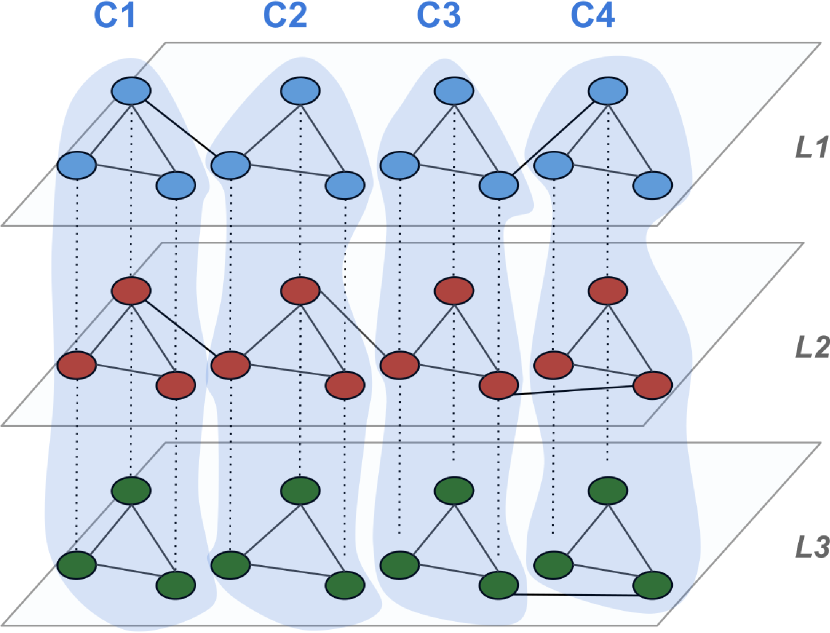
(a) Pillar Equal Partitioning (PEP)

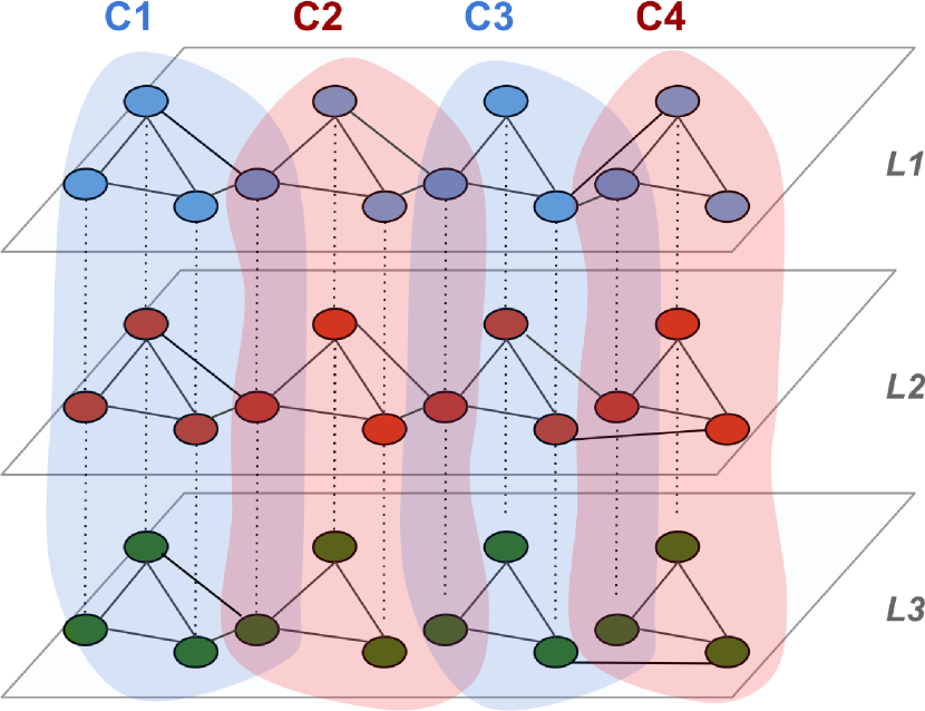
(b) Pillar Equal Overlapping (PEO)

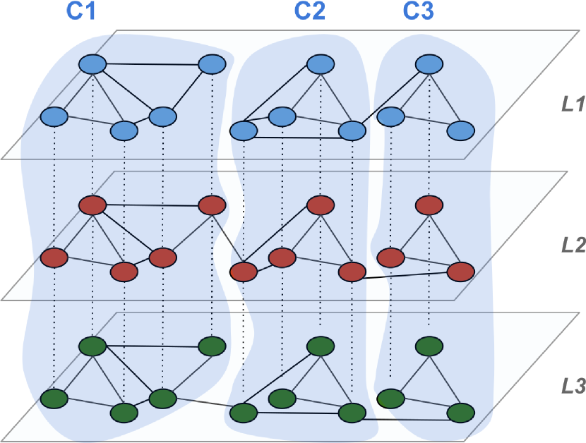
(c) Pillar Non-Equal Partitioning (PNP)

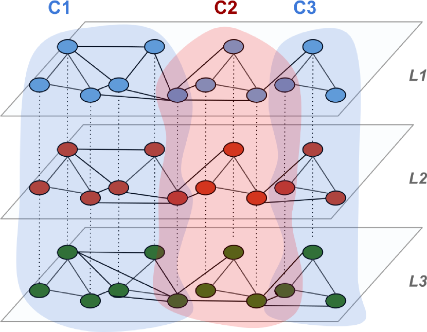
(d) Pillar Non-Equal Overlapping (PNO)

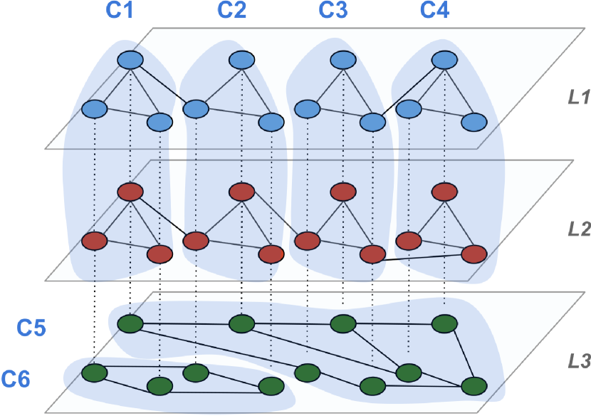
(e) Semi-pillar Equal Partitioning (SEP)

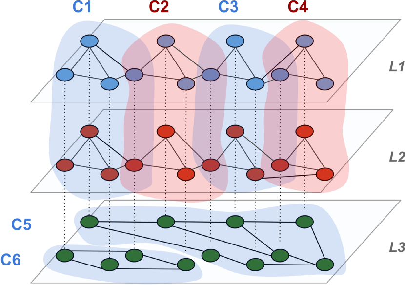
(f) Semi-pillar Equal Overlapping (SEO)

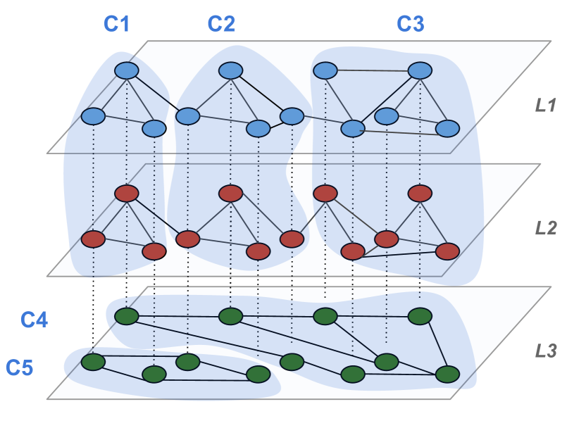
(g) Semi-pillar Non-equal Part. (SNP)

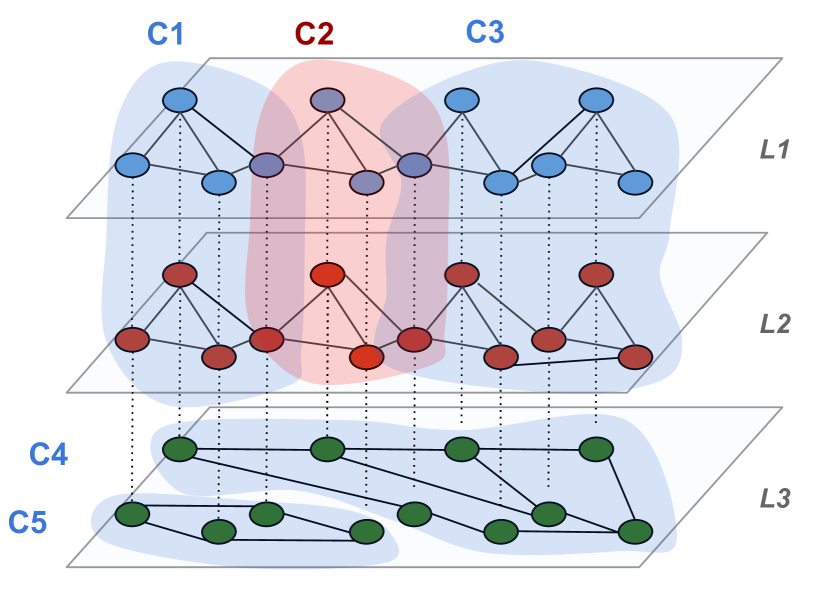
(h) Semi-pillar Non-equal Over. (SNO)

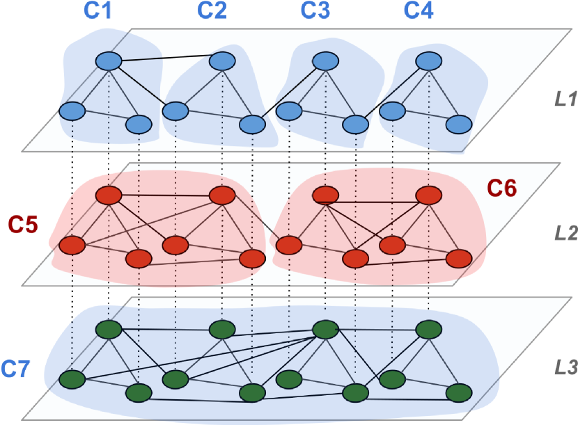
(i) Hierarchical (HIE)

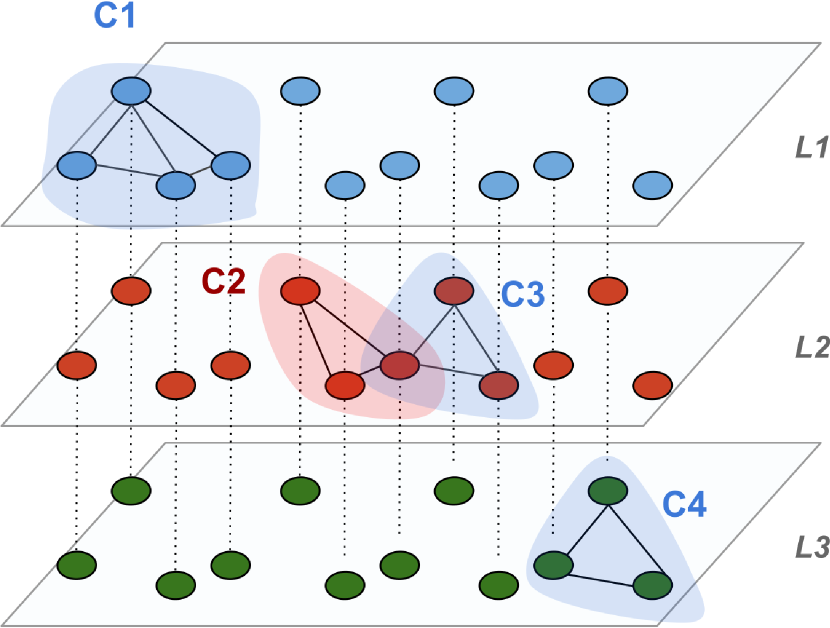
(j) Mixed (MIX)

Figure 8: An illustration of the types of synthetic multiplex networks generated for different possible multiplex community structures. Equal/Non-Equal refers to the number of nodes (size) in the communities

5.2 Detailed setting for each method

For all methods based on a single-layer algorithm, we use Louvain. Using the same algorithm makes the comparison fairer; however we must point out how this deviates from some original publications. We also tested the methods using the single-layer algorithm mentioned in the original references (e.g., label propagation). We think that the relevance of these methods for this paper lies in the way they deal with the multilayer structure rather than the specific algorithm that is used on the single-layer network. Within this perspective, using Louvain provides more stable, more accurate and more comparable results in general.

With respect to parameter setting, in general we used the default values proposed by the original works. In some specific cases, where different parameter settings are expected to be used to identify different types of community structures (i.e., GLouvain, ML-CPM, ABACUS, ACLcut, ML-LCD, and Infomap), we tested multiple settings as detailed in the following.

• For ABACUS, two main parameters have effect on filtering out possible multiplex communities when single-layer communities are merged into the final result, namely, the minimum number of actors in a community ($k$) and the minimum number of single-layer communities in which the actors must have been grouped together ($m$). We use this algorithm with two settings, ABACUS₃₁ with ($k$=3, $m$=1) and ABACUS₄₂ with ($k$=4, $m$=2) which filters out the communities that are not expanded over multiple layers.

• PMM takes three parameters: the number of communities to return, the number of structural features, and the number of times k-means should be executed as a subroutine, that we set to 5. The number of communities has been set to the number of known communities in the data where that is known, and to an arbitrary number (10) for Airports and Rattus. The fact that we used knowledge about the expected result to setup the algorithm should be considered when the different methods are compared. We did not find heuristics to set the number of structural features (Ell), so we used two settings: low and constant (Ell = 10), and high and dependent on the number of actors (Ell = $a/2$); these are among the settings returning good results for AUCS and PEP, for which a ground truth compatible with the results that PMM can return exists. However, please notice that the results may vary very significantly by varying this parameter, and we set it based on knowledge of the expected result. This should also be considered when looking at the experimental results.

• SCML takes two parameters: the number of communities, for which the same settings and reflections for PMM apply, and lambda, set to the default value .5.

• EMCD takes one parameter, theta, for which different settings can lead to significantly different results. The original reference contains an evaluation of appropriate ranges of theta for datasets with different statistics. We based our settings on these considerations: .03 for Airports and Rattus, .01 for DKPol, .2 for AUCS, .1 for the synthetic networks.

• ML-CPM: two main parameters can influence the results and the execution time of the algorithm, namely, the minimum number of actors that form a multilayer clique ($k$), and the minimum number of layers to be considered when counting the multilayer cliques ($m$). To be more inclusive, we defined two settings for these parameters, ML-CPM₃₁ with ($k$=3, $m$=1) which allows single-layer communities but could be computationally very expensive with large networks, and ML-CPM₄₂ with ($k$=4, $m$=2) which is less expensive computationally, but forces the communities to be expanded over at least two layers.

• LART has been executed with default parameter settings: $t=9$ (number of steps for random walker to take), eps = 1 (for binary matrices this will mean adding a self-loop to each node on each layer), gamma = 1 (recommended by the authors), and linkage = average (determining the type of hierarchical clustering performed in the algorithm).

• Infomap can be used to find both overlapping and non-overlapping communities. Consequently, we included it twice in our experiments, i.e., forcing a non-overlapping community discovery (Infomap_no), and accepting overlapping communities (Infomap_o).

• For GLouvain we defined two settings, GLouvain_h to denote high weight assigned to the inter-layer edges ($\omega=1$), and GLouvain_l to refer to a low value for the inter-layer edge weight ($\omega=0.1$). The motivation is that high values for $\omega$ favor the identification of pillar communities and may prevent the identification of actor-overlapping communities that the algorithm can retrieve with a low $\omega$.

• MLink takes two input parameters leading to different types of results. As we have not analyzed the resulting communities, for which we refer to the original reference, we use the default values used in the original implementation for scalability analysis.

• MDLPA has no input parameters.

• For ACLcut, two settings were used. One with a classical random walker ACLcut_c, and another with a relaxed random walker ACLcut_r.

• For ML-LCD we used three settings corresponding to different ways to optimize the $LC$ function during the selection of nodes to join a local community, namely, ML-LCD_(lwsim), for the layer-weighted similarity based $LC$, ML-LCD_(wlsim) for the within-layer similarity based $LC$, and ML-LCD_(clsim) for the cross-layer similarity based $LC$.

5.3 Software

The following experiments have been performed using a combination of original code (LART in Python2.7, EMCD in Java, PMM, SCML, and MLink in MATLAB, Infomap in C++) and the implementations of the other algorithms available in the multinet library (NWF, WF_EC, ABACUS, ML-CPM, GLouvain, MDLPA, all written in C++ and also available for R and Python). We also use the multinet library for basic functions to read networks, communities, to compute the Omega index, etc. Infomap was also run from inside multinet, but the code is the one from the authors with minor adaptations to make it compatible with the requirements of the CRAN repository. The implementation of ABACUS uses code from https://borgelt.net/eclat.html for the association rule mining subroutine. All the algorithms are available at https://bitbucket.org/uuinfolab/20csur, except ACLCut which has not been ported to the latest version of the multinet library. The MATLAB code in this repository is run using Octave. All the MATLAB code could be executed in Octave, except the internal edge clustering subroutine used by MLink. As we did not compare the results of Mlink with other algorithms, we skipped that part of the execution, which does not affect our conclusions about its scalability.

5.4 Assessment criteria

In order to measure pairwise similarity between two global community structures, we use the Omega index which is a well known measure [13] that can be applied to situations where both, one, or neither of the clusterings being compared is overlapping [42]. It does so by averaging the number of agreements on both clusterings and then adjusting that by the expected number of agreements between the two clusterings in case they were generated at random. An agreement is when two nodes are clustered together in the same number of clusters ($j$) in both clusterings. The values of $j$ start from 0, meaning that if two nodes are never clustered together in both clusterings, this still counts as an agreement.

Given two clusterings $\mathcal{C}_{1}$, $\mathcal{C}_{2}$, the similarity between them using Omega index is given by

$$\text{Omega ($\mathcal{C}_{1}$,$\mathcal{C}_{2}$)}=\frac{\text{Observed ($\mathcal{C}_{1}$,$\mathcal{C}_{2}$)}-\text{Expected ($\mathcal{C}_{1}$,$\mathcal{C}_{2}$)}}{1-\text{Expected ($\mathcal{C}_{1}$,$\mathcal{C}_{2}$)}}$$ (1)

$$\text{Observed ($\mathcal{C}_{1}$,$\mathcal{C}_{2}$)}=\frac{1}{N}\sum_{j=0}^{l}A_{j}$$ (2)

$$\text{Expected ($\mathcal{C}_{1}$,$\mathcal{C}_{2}$)}=\frac{1}{N^{2}}\sum_{j=0}^{l}N_{(j,1)}N_{(j,2)}$$ (3)

Where Observed ($\mathcal{C}_{1}$,$\mathcal{C}_{2}$) refers to the observed agreement represented by the average number of agreements between $\mathcal{C}_{1}$ and $\mathcal{C}_{2}$, $l$ is the maximum number of times a pair appears together in both $\mathcal{C}_{1}$ and $\mathcal{C}_{2}$ at the same time, N is the total number of possible pairs, $A_{j}$ is the number of pairs that are grouped together $j$ times in both clusterings, and $N_{(j,1)}$, $N_{(j,2)}$ indicate the numbers of pairs that have been grouped together $j$ times in $\mathcal{C}_{1}$, $\mathcal{C}_{2}$ respectively. Theoretically, values of the Omega index are in the range [-1,1]. However, in practice, Omega index returns 1 for two identical clusterings, and values close to 0 when one of the two input clusterings is a totally random reordering of the other one.

To clarify the formulas above, we provide two examples. First, to understand the meaning of each part of the formulas, consider two equal overlapping clusterings of four elements 1, 2, 3, and 4: $\mathcal{C}_{1}=\{\{1,2,3\},\{2,3,4\}\}$ and $\mathcal{C}_{2}=\{\{1,2,3\},\{2,3,4\}\}$. In this case the number of possible pairs $N$ is 6 ($\{1,2\},\{1,3\},\{1,4\}\dots$). $A_{0}=1$, because only the pair $\{1,4\}$ does not appear inside a same cluster in both clusterings. $A_{1}=4$, corresponding to pairs $\{1,2\},\{1,3\},\{2,4\}$, and $\{3,4\}$, all appearing together once in each clustering. Only the pair $\{2,3\}$ is assigned to two different clusters in each clustering, therefore $A_{2}=1$. The other values to compute the omega index are $N_{(0,1)}=1,N_{(0,2)}=1,N_{(1,1)}=4,N_{(1,2)}=4,N_{(2,1)}=1,N_{(2,2)}=1$. As a result, we have: $\text{Observed ($\mathcal{C}_{1}$,$\mathcal{C}_{2}$)}=\frac{1}{6}(1+4+1)$ and $\text{Expected ($\mathcal{C}_{1}$,$\mathcal{C}_{2}$)}=\frac{1}{36}(1\cdot 1+4\cdot 4+1\cdot 1)$. The corresponding Omega index is 1, as expected because the two clusterings are identical. Now consider the two clusterings $\mathcal{C}_{1}=\{\{1,2\},\{3,4\}\}$ and $\mathcal{C}_{2}=\{\{1,2\},\{3\},\{4\}\}$. We now have $\text{Observed ($\mathcal{C}_{1}$,$\mathcal{C}_{2}$)}=\frac{1}{6}(4+1)$ and $\text{Expected ($\mathcal{C}_{1}$,$\mathcal{C}_{2}$)}=\frac{1}{36}(4\cdot 5+2\cdot 1)$ with Omega index 0.57.

The reason why we choose the Omega index is that it is, by definition, a valid measure when one, both or none of the two clusterings is overlapping as we discuss in [22]. In addition, Omega index is an adjusted similarity measure that accounts for the by-chance agreements that might still exist between any two random clusterings over the same node-set.

For measuring similarity between two local communities $s_{1}$, $s_{2}$, we use the Jaccard coefficient:

$$JC=\frac{N(s_{1},s_{2})}{N(s_{1})+N(s_{2})-N(s_{1},s_{2})}$$ (4)

where $N(s_{1})$ refers to the number of actors in solution $s_{1}$ and $N(s_{1},s_{2})$ refers to the number of common actors between two solutions $s_{1}$, $s_{2}$. The values of the Jaccard coefficient lie in the range [0,1] where 1 means perfect similarity and 0 means perfect dissimilarity.

In order to measure the accuracy of the solutions obtained by global methods with respect to a ground truth (Section 6.1.2), we resort again to the Omega index. The accuracy of local community detection methods (Section 6.2.1) has been evaluated by comparing pairwise similarities (using the Jaccard index) between a given actor (i.e., seed node) and the ground truth community it belongs to. The average Jaccard index over all actors is then used as the final accuracy score.

6 Results

In this section we present the experimental results of our comparative evaluation. Results of the comparative evaluation of global methods are reported in Section 6.1, while results related to the evaluation of local methods are reported in Section 6.2.

6.1 Global Methods

In this section we report the experimental results of the comparative evaluation of global multiplex community detection methods. The section is structured as follows: Section 6.1.1 reports on the main properties of the community structures detected by the evaluated methods in different datasets. Section 6.1.2 presents the results of the accuracy analysis. Section 6.1.3 discusses the results of the pairwise comparison between different methods. Section 6.1.4 focuses on scalability.

6.1.1 Basic descriptive statistics

As the first step of our comparative analysis, we analyzed the structural properties of the different community structures identified by the evaluated methods. Tables 6.1.1 and 6.1.1 present the statistics concerning the community structures obtained on the smallest (AUCS) and largest (Airports) of the real-world multiplex networks taken into account. We also present the general statistics about the communities detected on DKPol and Rattus datasets in Tables 6.1.1 and 6.1.1. Statistics of each method occupy one row in each a table (multiple settings of the input parameters for some methods are represented as separated entries for the same method). Since some of the methods are non-deterministic, we executed each method 10 times, and provide mean and standard deviation.

It can be observed how LART generates a number of communities which is higher than that of most other methods on all real networks. However a large percentage of these communities appear to be singletons, indicating that this algorithm mostly fails in aggregating nodes into communities. Other algorithms which appear to generate a relatively high number of communities regardless of the network structure are Infomap_o and ABACUS, both variants. Interestingly, both retrieve a large number of communities without retrieving any singleton, showing a different behavior from LART. The discovery of many communities by Infomap_o and ABACUS is associated to a high percentage of node overlapping. As regards to the size of the largest community, higher values correspond to PMM_l and Infomap_o. On the other end, ABACUS (both variants) and ML-CPM₄₂ assign a small number of nodes to the largest communities, in both the AUCS and the Airports networks. This can be explained by the strong requirements that ABACUS and (even more) ML-CPM have to cluster nodes together. Concerning $sc2/sc1$, we can observe how the values tend to be all relatively high for the smallest (AUCS) and largest (Airports) networks, indicating that in these cases the largest communities for each identified community structure have comparable sizes. An algorithm grouping most of the nodes together, and thus not able to structure them into separate communities, would have a very low value for $sc2/sc1$.

The values found in columns $\%n$, $\%p$, $\%ao$ and $\%no$ can be explained as follows:

• With regards to the percentage $\%n$ of nodes assigned to at least one community, as we discussed in Section 2, certain methods are forced to provide a community assignment for each node: in these cases the value of $\%n$ will always be $1$.

• Regarding the percentage $\%p$ of pillars, both flattening methods always return pillar communities (since the information about layers is lost during the flattening process). Infomap and GLouvain can detect non-pillar clusters in theory. Data show how Infomap can return non-pillars both in the overlapping and in the non-overlapping version, while only GLouvain_l returns non-pillar communities.

• The percentage of overlapping actors ($\%ao$) and nodes ($\%no$) mainly depends on the properties of the specific methods whether they allow overlapping (on the node level or the actor level) or not.

• The percentage of singleton communities $\%s$ appears to be extremely high in the case of LART and EMCD and high in the case of PMM_l. It should be noted that, with the exception of Infomap, that returns a small fraction of singletons in the Airports network, the methods that return singletons in the AUCS network return a larger percentage of singletons in the Airports network suggesting that the behaviour is not induced by the network but amplified by its complexity.

Table 5: Statistics about the community structures obtained on the AUCS network (results averaged over 10 runs). We denote with #c the number of communities, with sc1 the size of the largest community (number of nodes), with sc2/sc1 the ratio between the size of the second largest community and the largest, with %n the percentage of nodes assigned to at least one community, with %p the percentage of pillars, with %ao the percentage of actors in more than one community, with %no the percentage of nodes in more than one community and with %s the percentage of singleton communities

method	$\#c$	$sc1$	$sc2/sc1$	$\%n$	$\%p$	$\%ao$	$\%no$	$\%s$
NWF	$5.00$	$75.00$	$0.92$ p m 0.01	$1.00$	$1.00$	$0.00$	$0.00$	$0.00$
WFEC	$5.00$	$75.00$	$0.92$ p m 0.01	$1.00$	$1.00$	$0.00$	$0.00$	$0.00$
ABACUS31	$46.50$ p m 3.44	$29.90$ p m 2.54	$0.96$ p m 0.02	$0.70$	$0.00$	$0.96$	$0.61$	$0.00$
ABACUS42	$25.50$ p m 3.58	$29.20$ p m 2.52	$0.96$ p m 0.03	$0.59$ p m 0.01	$0.00$	$0.67$ p m 0.01	$0.39$ p m 0.01	$0.00$
EMCD	$11.00$	$70.00$	$0.92$	$1.00$	$1.00$	$0.00$	$0.00$	$0.45$
PMMl	$8.00$	$103.00$ p m 21.00	$0.49$ p m 0.14	$1.00$	$1.00$	$0.00$	$0.00$	$0.05$ p m 0.08
PMMh	$8.00$	$79.50$ p m 16.94	$0.75$ p m 0.17	$1.00$	$1.00$	$0.00$	$0.00$	$0.02$ p m 0.05
SCML	$8.00$	$66.00$ p m 3.00	$0.94$ p m 0.11	$1.00$	$1.00$	$0.00$	$0.00$	$0.00$
ML-CPM31	$40.00$	$59.00$	$0.61$	$0.61$	$0.00$	$0.93$	$0.46$	$0.00$
ML-CPM42	$11.00$	$18.00$	$0.88$	$0.27$	$0.00$	$0.34$	$0.11$	$0.00$
LART	$48.60$ p m 0.66	$51.00$ p m 2.00	$0.58$ p m 0.02	$1.00$	$0.98$	$0.01$	$0.00$	$0.91$
Infomapno	$5.09$ p m 0.30	$86.00$ p m 8.30	$0.80$ p m 0.06	$1.00$	$1.00$	$0.00$	$0.00$	$0.00$
Infomapo	$20.60$ p m 0.80	$157.00$ p m 44.00	$0.49$ p m 0.12	$1.00$	$0.30$ p m 0.02	$0.69$ p m 0.02	$0.69$ p m 0.02	$0.00$
GLouvainl	$7.50$ p m 0.67	$80.20$ p m 7.34	$0.85$ p m 0.08	$1.00$	$0.44$ p m 0.08	$0.55$ p m 0.08	$0.00$	$0.00$
GLouvainh	$5.00$	$76.50$ p m 4.50	$0.85$ p m 0.04	$1.00$	$1.00$	$0.00$	$0.00$	$0.00$
MDLPA	$6.70$ p m 0.78	$87.50$ p m 18.74	$0.65$ p m 0.17	$1.00$	$1.00$	$0.00$	$0.00$	$0.00$

(a) AUCS. l = 5, a = 61, e = 620

Table 6: Statistics about the community structures obtained on the Airports network (results averaged over 10 runs). We denote with #c the number of communities, with sc1 the size of the largest community (number of nodes), with sc2/sc1 the ratio between the size of the second largest community and the largest, with %n the percentage of nodes assigned to at least one community, with %p the percentage of pillars, with %ao the percentage of actors in more than one community, with %no the percentage of nodes in more than one community and with %s the percentage of singleton communities

method	$\#c$	$sc1$	$sc2/sc1$	$\%n$	$\%p$	$\%ao$	$\%no$	$\%s$
NWF	$6.80$ p m 0.60	$4229.10$ p m 653.56	$0.77$ p m 0.16	$1.00$	$1.00$	$0.00$	$0.00$	$0.00$
WFEC	$6.70$ p m 0.45	$4417.80$ p m 532.90	$0.73$ p m 0.11	$1.00$	$1.00$	$0.00$	$0.00$	$0.00$
ABACUS31	$5320.30$ p m 89.42	$84.00$	$0.95$	$0.12$	$0.00$	$0.63$	$0.10$	$0.00$
ABACUS42	$4086.40$ p m 69.71	$84.00$	$0.95$	$0.09$	$0.00$	$0.32$ p m 0.01	$0.07$	$0.00$
EMCD	$314.00$	$2035.00$	$0.30$	$1.00$	$1.00$	$0.00$	$0.00$	$0.97$
PMMl	$10.00$	$14\,289.40$ p m 246.98	$0.03$ p m 0.01	$1.00$	$1.00$	$0.00$	$0.00$	$0.48$ p m 0.15
PMMh	$10.00$	$2171.90$ p m 153.49	$0.86$ p m 0.07	$1.00$	$1.00$	$0.00$	$0.00$	$0.00$
SCML	$10.00$	$4336.39$ p m 1128.68	$0.46$ p m 0.21	$1.00$	$1.00$	$0.00$	$0.00$	$0.00$
ML-CPM31	$62.00$	$93.00$	$0.72$	$0.04$	$0.00$	$0.35$	$0.00$	$0.00$
ML-CPM42	$3.00$	$8.00$	$1.00$	$0.00$	$0.00$	$0.00$	$0.00$	$0.00$
Infomapno	$7.70$ p m 1.55	$10\,330.40$ p m 4920.32	$0.17$ p m 0.22	$0.80$ p m 0.35	$0.79$ p m 0.35	$0.00$	$0.00$	$0.08$ p m 0.10
Infomapo	$34.10$ p m 2.02	$6034.70$ p m 993.70	$0.83$ p m 0.11	$1.00$	$0.36$	$0.63$	$0.63$	$0.00$
GLouvainl	$11.20$ p m 0.60	$6161.80$ p m 382.63	$0.35$ p m 0.06	$1.00$	$0.50$	$0.49$	$0.00$	$0.00$
GLouvainh	$9.50$ p m 1.11	$5372.40$ p m 333.32	$0.57$ p m 0.13	$1.00$	$1.00$	$0.00$	$0.00$	$0.00$

(a) Airports. l = 37, a = 417, e = 3588

Table 7: Statistics about the community structures obtained on the DKPol network (results averaged over 10 runs). We denote with #c the number of communities, with sc1 the size of the largest community (number of nodes), with sc2/sc1 the ratio between the size of the second largest community and the largest, with %n the percentage of nodes assigned to at least one community, with %p the percentage of pillars, with %ao the percentage of actors in more than one community, with %no the percentage of nodes in more than one community and with %s the percentage of singleton communities. ML-CPM₃₁ is not present because it takes too long to produce a result, for all executions.

method	$\#c$	$sc1$	$sc2/sc1$	$\%n$	$\%p$	$\%ao$	$\%no$	$\%s$
NWF	$6.30$ p m 0.90	$370.50$ p m 40.56	$0.93$ p m 0.06	$1.00$	$1.00$	$0.00$	$0.00$	$0.00$
WFEC	$6.30$ p m 1.10	$378.60$ p m 39.04	$0.90$ p m 0.07	$1.00$	$1.00$	$0.00$	$0.00$	$0.00$
ABACUS31	$69.40$ p m 2.05	$123.50$ p m 17.02	$0.92$ p m 0.05	$0.55$	$0.00$	$0.44$	$0.32$	$0.00$
ABACUS42	$31.20$ p m 2.44	$65.20$ p m 2.22	$0.92$ p m 0.05	$0.30$ p m 0.01	$0.00$	$0.11$ p m 0.01	$0.07$	$0.00$
EMCD	$14.00$	$279.00$	$0.77$	$1.00$	$1.00$	$0.00$	$0.00$	$0.00$
PMMl	$9.00$	$992.40$ p m 52.98	$0.12$ p m 0.02	$1.00$	$1.00$	$0.00$	$0.00$	$0.07$ p m 0.07
PMMh	$9.00$	$217.20$ p m 25.84	$0.94$ p m 0.05	$1.00$	$1.00$	$0.00$	$0.00$	$0.00$
SCML	$9.00$	$256.50$ p m 34.63	$0.80$ p m 0.05	$1.00$	$1.00$	$0.00$	$0.00$	$0.00$
ML-CPM42	$9.00$	$24.00$	$0.91$	$0.06$	$0.00$	$0.00$	$0.00$	$0.00$
Infomapno	$1.00$	$1470.00$	$1.00$	$1.00$	$1.00$	$0.00$	$0.00$	$0.00$
Infomapo	$23.00$ p m 5.77	$1470.00$	$0.27$ p m 0.11	$1.00$	$0.65$ p m 0.09	$0.34$ p m 0.09	$0.34$ p m 0.09	$0.45$ p m 0.06
GLouvainl	$19.50$ p m 0.80	$347.60$ p m 42.45	$0.87$ p m 0.05	$1.00$	$0.65$ p m 0.01	$0.34$ p m 0.01	$0.00$	$0.02$ p m 0.02
GLouvainh	$7.60$ p m 0.66	$303.89$ p m 11.14	$0.93$ p m 0.02	$1.00$	$1.00$	$0.00$	$0.00$	$0.00$
MDLPA	$1.00$	$1470.00$	$1.00$	$1.00$	$1.00$	$0.00$	$0.00$	$0.00$

(a) DKPol. l = 3, a = 493, e = 20226

Table 8: Statistics about the community structures obtained on the Rattus network (results averaged over 10 runs). We denote with #c the number of communities, with sc1 the size of the largest community (number of nodes), with sc2/sc1 the ratio between the size of the second largest community and the largest, with %n the percentage of nodes assigned to at least one community, with %p the percentage of pillars, with %ao the percentage of actors in more than one community, with %no the percentage of nodes in more than one community and with %s the percentage of singleton communities. ML-CPM₄₂ is not present because it does not find any community.

method	$\#c$	$sc1$	$sc2/sc1$	$\%n$	$\%p$	$\%ao$	$\%no$	$\%s$
NWF	$136.10$ p m 0.94	$3264.60$ p m 15.97	$0.38$ p m 0.01	$1.00$	$1.00$	$0.00$	$0.00$	$0.04$
WFEC	$135.40$ p m 1.20	$3260.40$ p m 18.82	$0.40$ p m 0.06	$1.00$	$1.00$	$0.00$	$0.00$	$0.04$
ABACUS31	$199.70$ p m 3.19	$544.60$ p m 1.20	$0.27$ p m 0.05	$0.18$	$0.00$	$0.15$	$0.02$	$0.00$
ABACUS42	$23.70$ p m 1.55	$29.60$ p m 2.15	$0.91$ p m 0.06	$0.01$	$0.00$	$0.00$	$0.00$	$0.00$
EMCD	$219.00$	$3306.00$	$0.23$	$1.00$	$1.00$	$0.00$	$0.00$	$0.02$
PMMl	$10.00$	$12\,965.40$ p m 1963.48	$0.21$ p m 0.18	$1.00$	$1.00$	$0.00$	$0.00$	$0.14$ p m 0.06
PMMh	$10.00$	$1864.80$ p m 99.31	$0.94$ p m 0.03	$1.00$	$1.00$	$0.00$	$0.00$	$0.00$
ML-CPM31	$63.00$	$219.00$	$0.03$	$0.02$	$0.00$	$0.01$	$0.00$	$0.00$
Infomapo	$293.70$ p m 4.02	$10\,336.20$ p m 409.14	$0.12$ p m 0.06	$1.00$	$0.81$	$0.18$	$0.18$	$0.04$
GLouvainl	$163.80$ p m 2.44	$3258.50$ p m 30.33	$0.29$ p m 0.06	$1.00$	$0.89$	$0.10$	$0.00$	$0.03$
GLouvainh	$137.19$ p m 1.16	$3261.00$ p m 17.02	$0.37$ p m 0.05	$1.00$	$1.00$	$0.00$	$0.00$	$0.04$
MDLPA	$287.80$ p m 12.55	$4411.80$ p m 533.45	$0.18$ p m 0.02	$1.00$	$1.00$	$0.00$	$0.00$	$0.03$

(a) Rattus. l = 6, a = 2640, e = 3956

6.1.2 Accuracy analysis

With the aim of answering Q1 (i.e., “To what extent are the evaluated methods able to detect ground truth communities?”, cf. Section 5), we perform here an extensive quantitative analysis about the accuracy obtained by each method with respect to ground truth communities. For real-world networks, only two of them have an available ground truth: AUCS (i.e., affiliations to research groups) and DKPol (i.e., affiliation to political parties). All synthetic networks come with controlled ground truth.

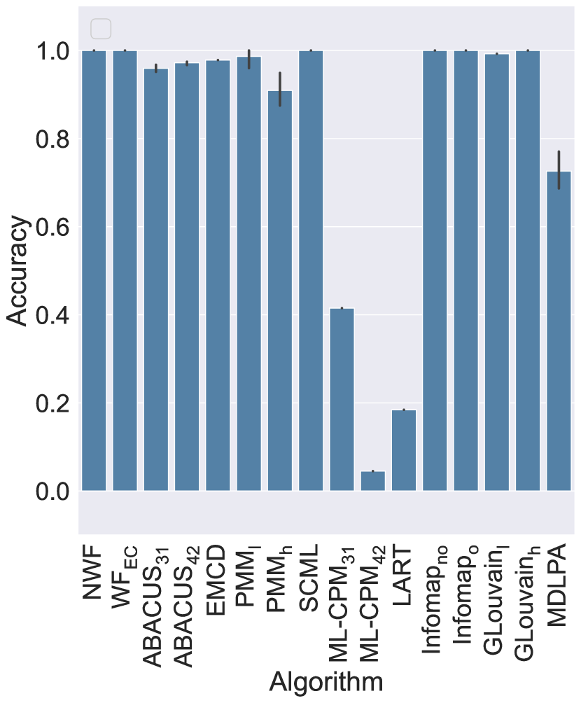
(a) Pillar Equal Partitioning (PEP)

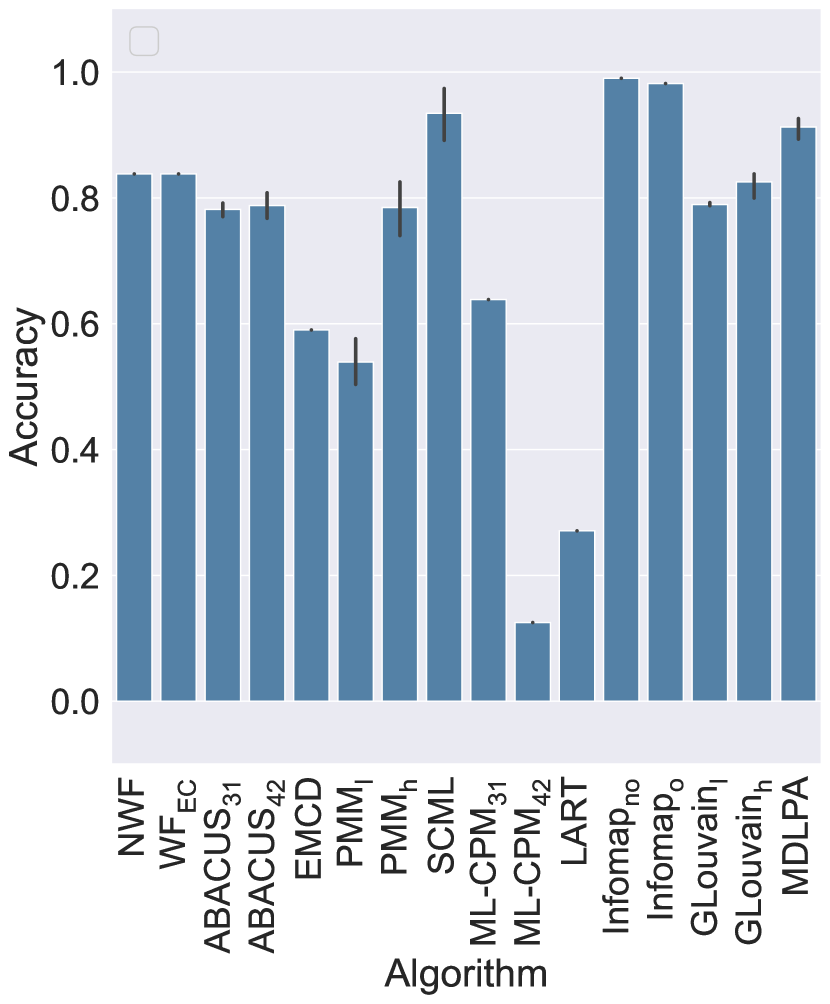
(b) Pillar Non-equal Partitioning (PNP)

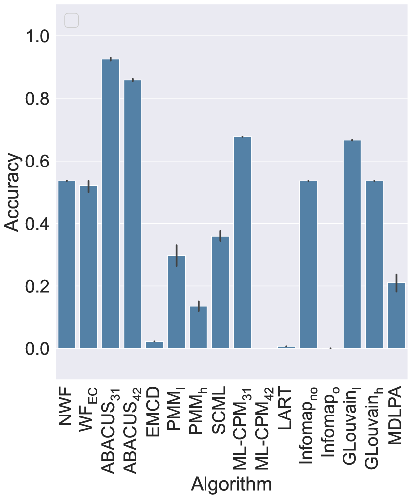
(c) Semi-pillar Equal Partitioning (SEP)

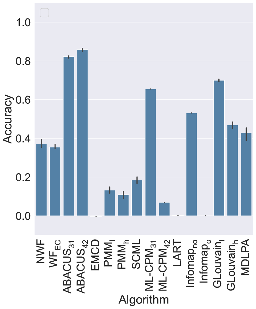
(d) Semi-pillar Non-equal Partitioning (SNP)

Figure 9: Accuracy with respect to a ground truth, Omega index, pillar communities (100 actors)

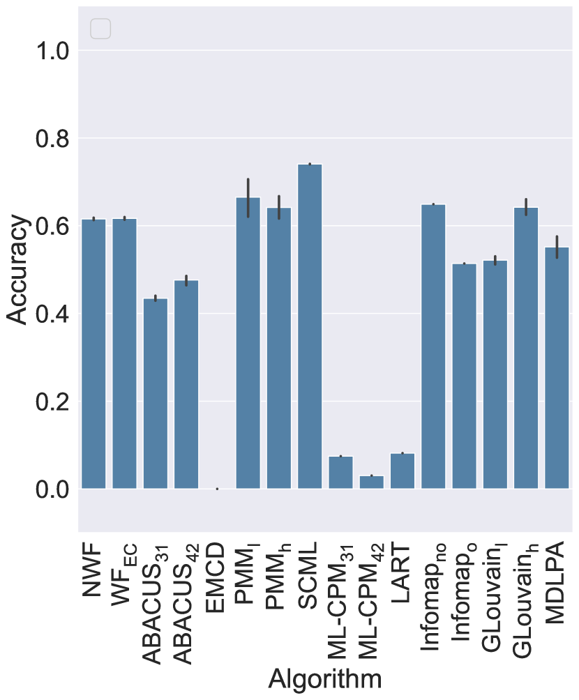
(a) Pillar Equal Overlapping (PEO)

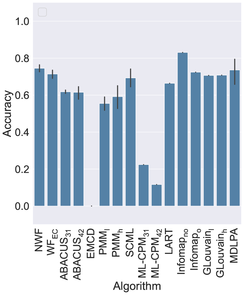
(b) Pillar Non-equal Overlapping (PNO)

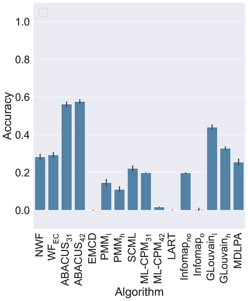
(c) Semi-pillar Equal Overlapping (SEO)

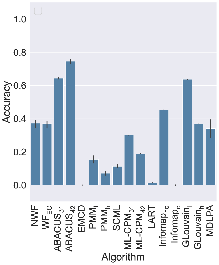
(d) Semi-pillar Non-equal Overlapping (SEO)

Figure 10: Accuracy with respect to a ground truth, Omega index, overlapping communities (100 actors)

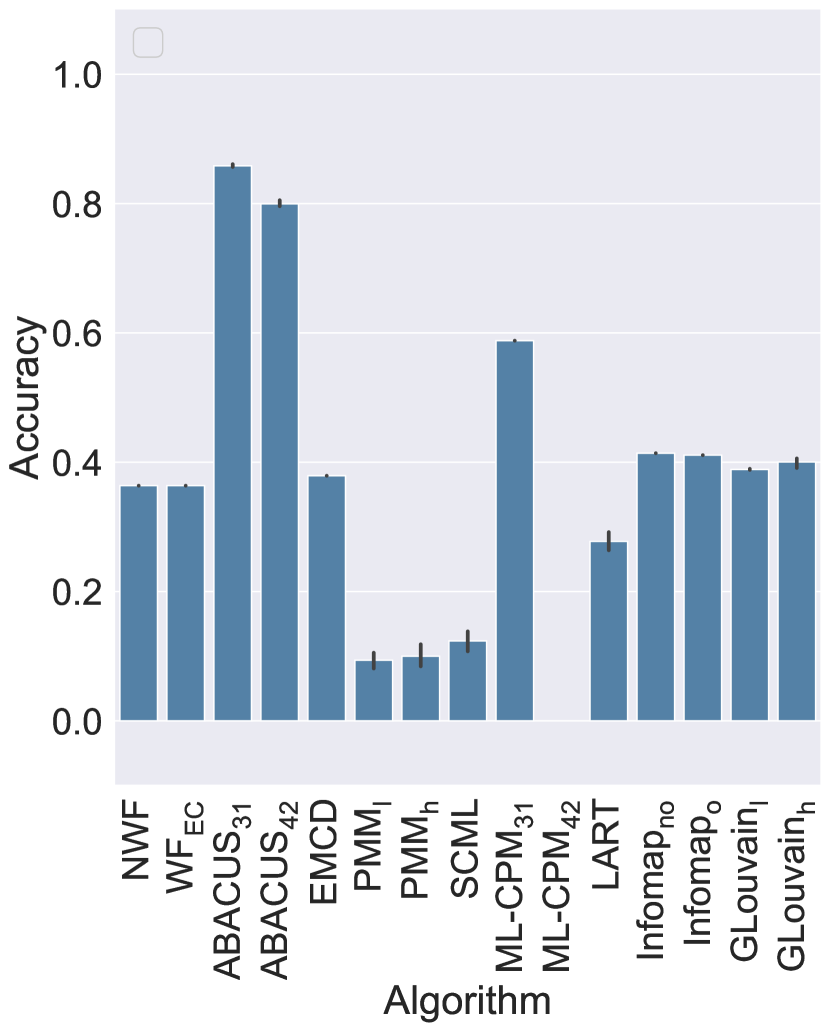
(a) Mixed (MIX)

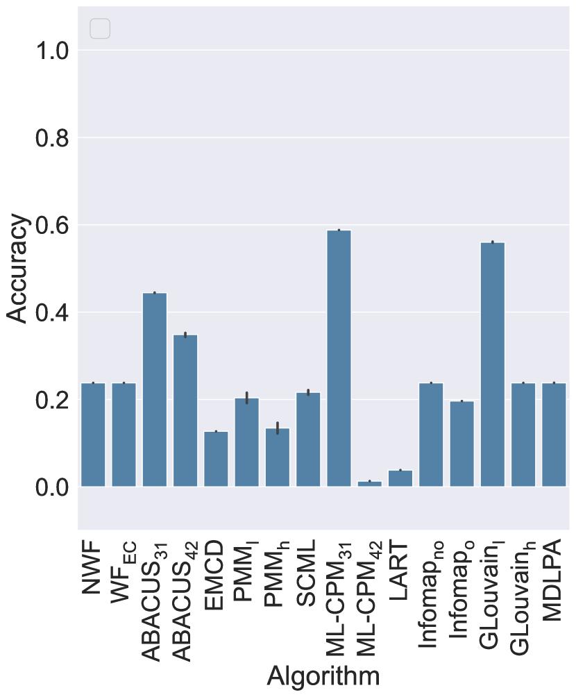
(b) Hierarchical (HIE)

Figure 11: Accuracy with respect to a ground truth, Omega index, mixed and hierarchical communities (100 actors)

Our results on networks with 100 actors are reported in Figures 9, 10, 11, while 12 shows results on real networks. At the end of this section we also show results on larger networks, which generally confirm these results highlighting a few additional behaviors. From these figures we can see how the main element playing a role in determining the accuracy of the methods is the pillar nature of the community structure.

In the case of Pillar Equal Partitioning (PEP) structures almost all the methods perform very well, with WF_EC, NWF, Infomap and GLouvain (both versions) reaching perfect accuracy. Overall, only ML-CPM (both versions) and LART score below 0.5. In the first case, the strict rules imposed by its parameters explain the performance, for the latter, as we saw in Table 6.1.1 LART does not seem to be able to group a considerable number of nodes into communities. Similar patterns, even if with worse levels of accuracy, are visible for all the Pillar structures (PNP, PEO, PNO). Minor notable differences are present in the Pillar Non-equal Partitioning structure where Infomap (both variations) performs better than all the other methods (that also score above $0.8$). Despite the positive results for many methods, one could easily ask if in the general context of pillar community structures proper multilayer methods are necessary since the same (good) results can be achieved with flattening-based methods.

The more the network moves away from a pillar structure (with semi-pillar, mixed and hierarchical structures) the worse the results are among most of the methods. A notable exception is ABACUS that, regardless of the variation, keeps performing above the average with Semi-Pillar and Mixed Communities, with ML-CPM₃₁ also performing better than most other methods on Semi-Pillar structures. Hierarchical structures are extremely challenging for all the methods with the notable exceptions of ML-CPM₃₁ and GLouvain_l, although GLouvain is finding communities on individual layers and thus it is not clearly identifying any hierarchy spanning multiple layers.

The reason why some methods have an Omega index around 0 is that in these cases these methods only find one or two large communities. This is not surprising if we consider the structures of some synthetic datasets. In the overlapping community structures all the communities are kept together by their overlapping parts, and in the semi-pillar structures the well-separated semi-pillar communities spanning a subset of the layers result connected by the different communities on the remaining layers.

These results may indicate that, even though for simple Pillar Equal Partitioning structures multilayer methods do not seem to provide any real advantage over flattening-based methods, more complex structures show how proper multilayer methods can perform better than flattening-based methods.

Figure 12 reports on the accuracy obtained by the evaluated methods on real-world networks. It can be observed how accuracy values are relatively low on both networks for all methods, i.e., with Omega index always below $0.8$ and often below $0.5$. More interestingly, the best performing methods do not entirely overlap with the methods that perform the best with the synthetic data. On AUCS, the best performing method is SCML ($0.70$), followed by EMCD.

The results are even more variable on DKPol, where many methods show low results. An exception to this are the two variants of GLouvain, reaching accuracies of $0.68$ (GLouvain_h) and $0.43$ (GLouvain_l) respectively. SCML, NWF, WF_EC and EMCD also perform relatively well with scores around $0.6$.

As a final remark, the difference in performance between real-world and synthetic networks confirms how the “ideal” concept of community, i.e., the one based on topological density that is used to build the synthetic ones and to drive the detection process of the methods, is often far from the ground truth communities observed in real cases (which are, in turn, often questionable and subjective). This is a well known problem in the community detection field, and poses challenges in both ways, i.e., concerning the need to design both more powerful methods and more reliable ground truths.

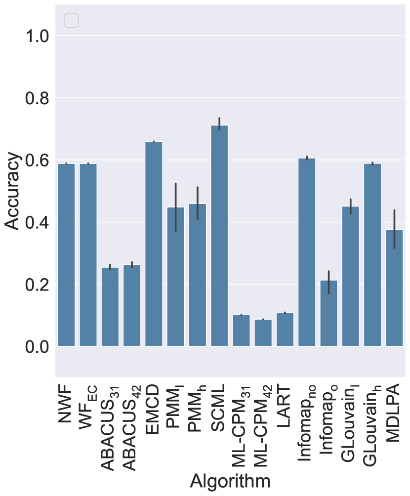
(a) AUCS

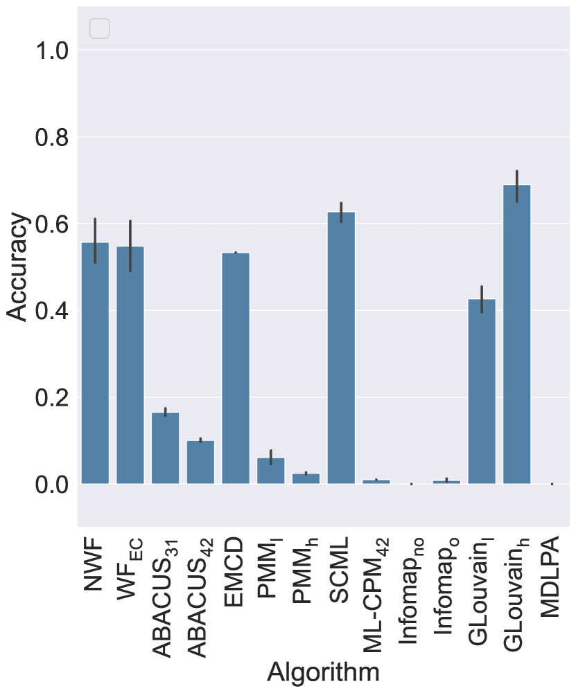
(b) DKPol

Figure 12: Accuracy with respect to a ground truth for real-world networks, measured using Omega index

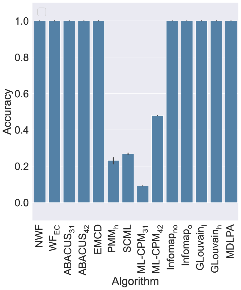
(a) Pillar Equal Partitioning (PEP)

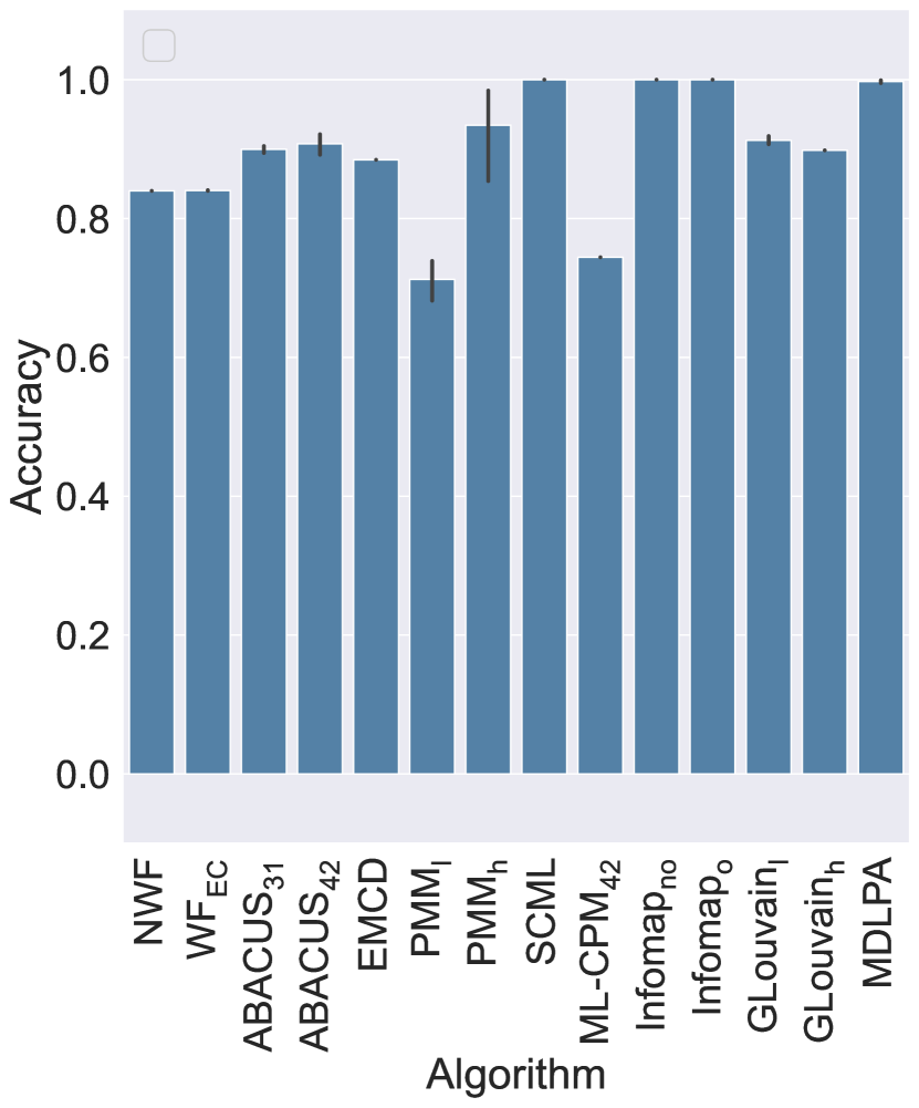
(b) Pillar Non-equal Partitioning (PNP)

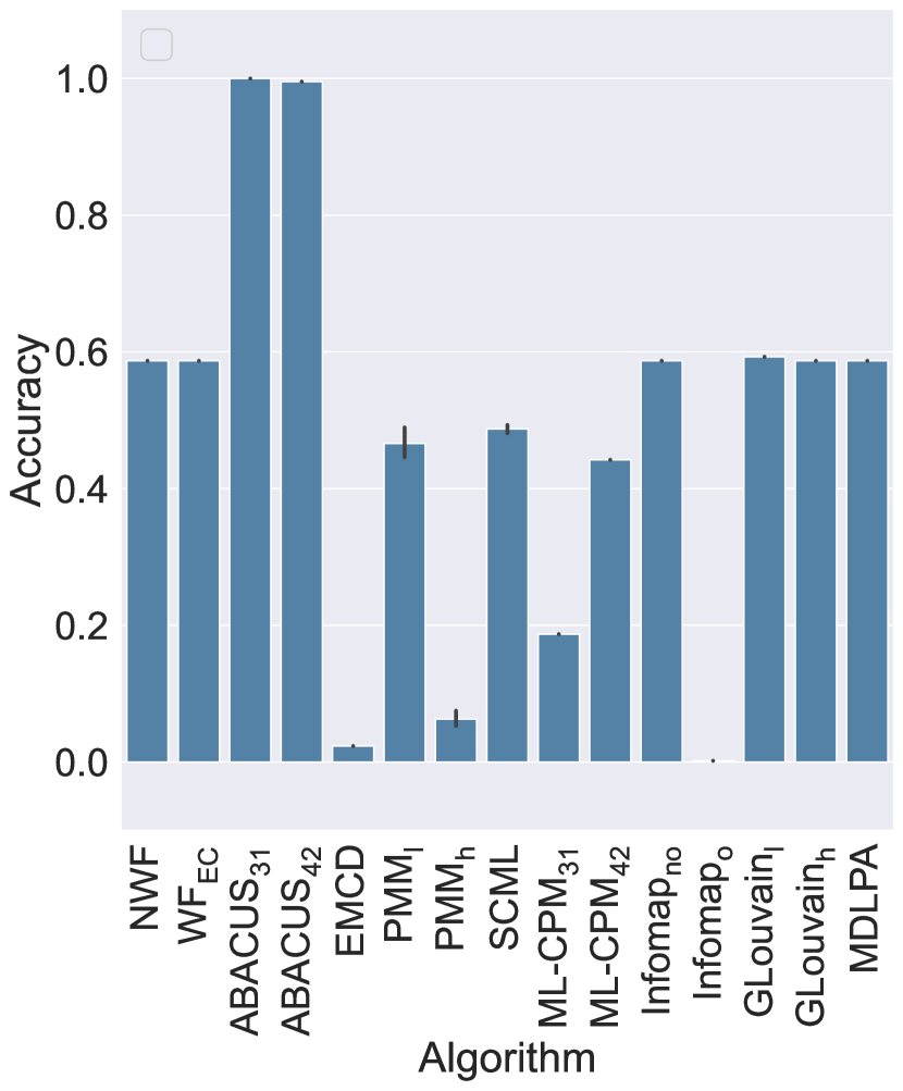
(c) Semi-pillar Equal Partitioning (SEP)

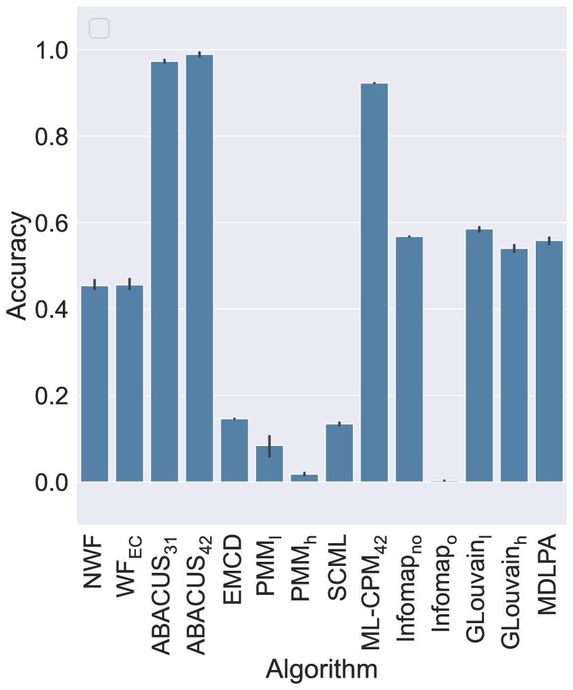
(d) Semi-pillar Non-equal Partitioning (SNP)

Figure 13: Accuracy with respect to a ground truth, Omega index, pillar communities (500 actors)

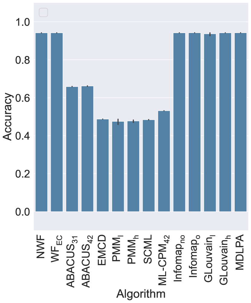
(a) Pillar Equal Overlapping (PEO)

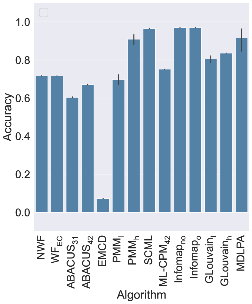
(b) Pillar Non-equal Overlapping (PNO)

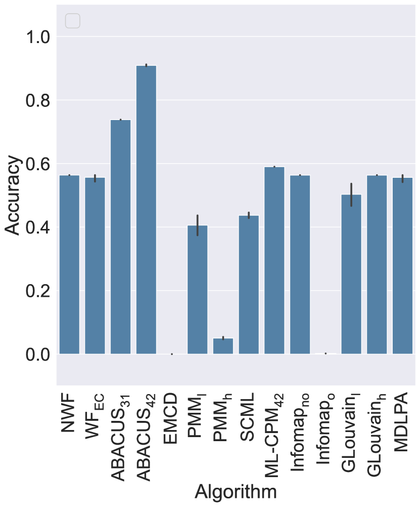
(c) Semi-pillar Equal Overlapping (SEO)

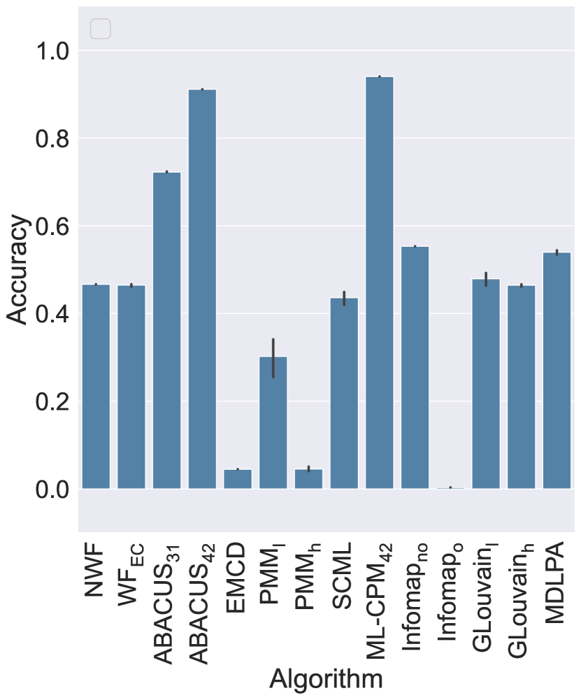
(d) Semi-pillar Non-equal Overlapping (SEO)

Figure 14: Accuracy with respect to a ground truth, Omega index, overlapping communities (500 actors)

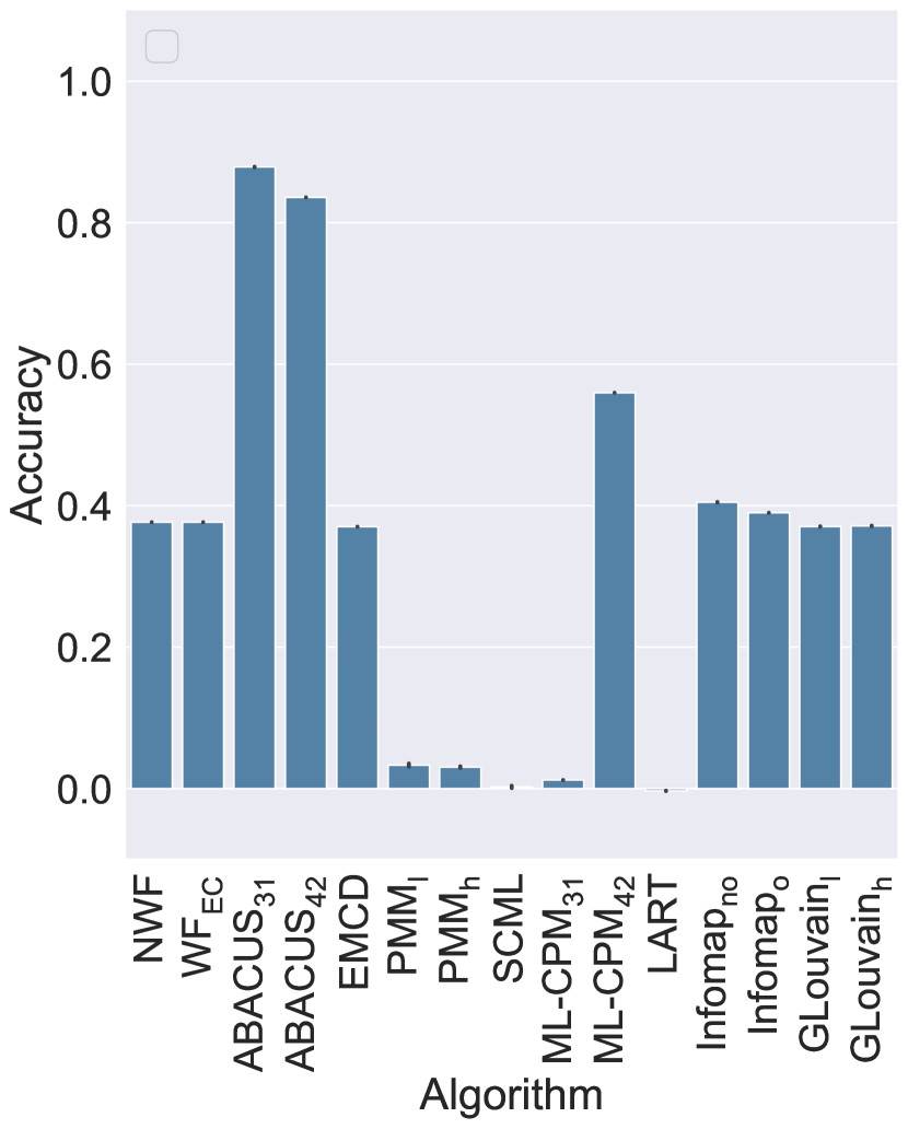
(a) Mixed (MIX)

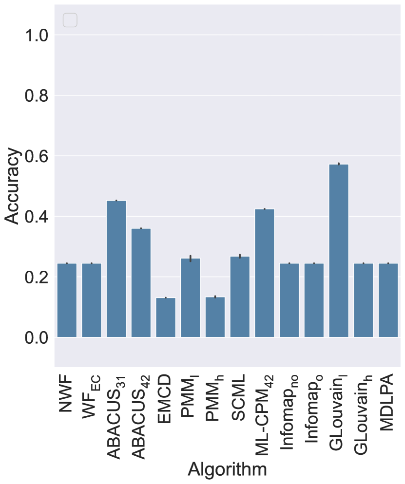
(b) Hierarchical (HIE)

Figure 15: Accuracy with respect to a ground truth, Omega index, mixed and hierarchical communities (500 actors)

Figures 13, 14, and 15 show the results of similar experiments on synthetic networks using larger networks. While small networks allowed us to obtain results also with more computationally expensive methods, a potential problem with small networks with communities of 10 actors is that the random generation of edges may increase noise on specific communities. The results are still very similar to the ones with smaller networks, with three main differences. First, some methods (PMM and SCML) show some instability, returning worse results in specific cases. Second, ML-CPM starts working better in the version with a larger minimum clique size. Third, we can see some general improvements in particular in the Pillar Equal Overlapping results, while still confirming the worsening patterns highlighted by the previous experiments when we move to Semi-Pillar and Non-Equal communities.

6.1.3 Pairwise comparison analysis

In order to answer Q2 (i.e., “To what extent do the evaluated methods produce similar community structures?”, cf. Section 5), we performed pairwise comparisons between the selected methods, in order to determine the similarity between the community structures produced by each pair of methods on each network.

Figure 16 reports on the results of pairwise analysis among Pillar Equal Partitioning and Semi-Pillar Non-equal Partitioning, with Omega index values for the pairwise similarities. We show Omega index values for a matter of homogeneity, since NMI cannot be applied to overlapping solutions.

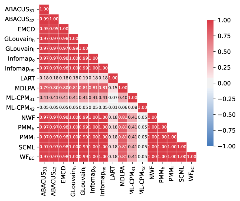
(a) PEP

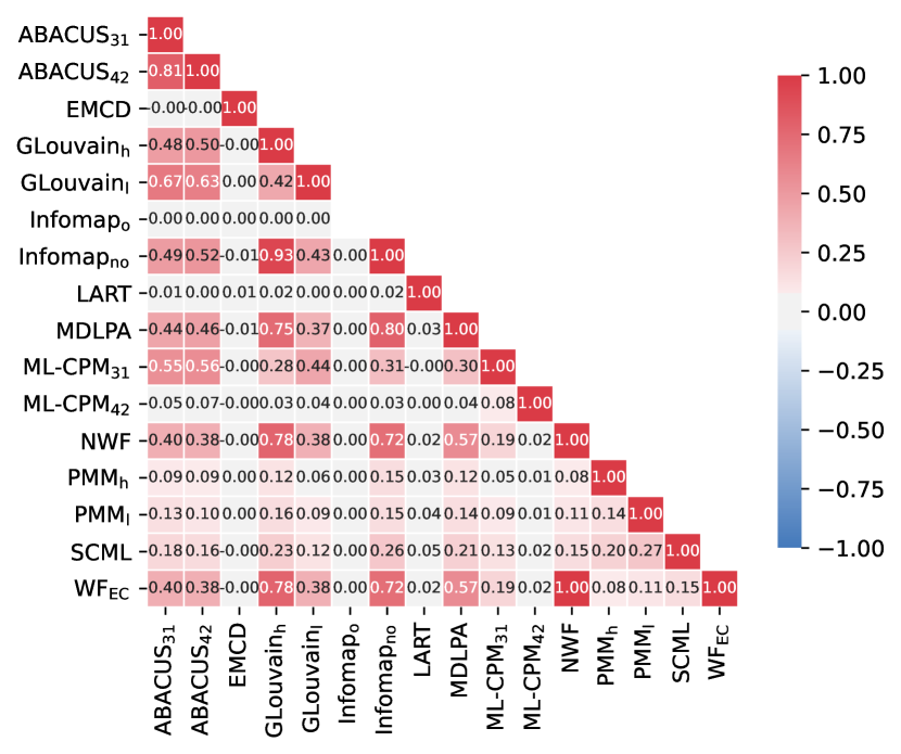
(b) SNP

Figure 16: Pairwise comparison, Omega index: pillar and semi-pillar partitioning communities

These results confirm and expand the understanding of the methods we have described so far. In the case of Pillar Equal Partitioning networks, almost all the methods produce very similar structures, with the notable exception of ML-CPM and LART. In the case of Semi-Pillar Partitioning communities the similarities are much smaller with few notable exceptions: Infomap_no returns communities extremely similar to those returned by GLouvain_h and both also show a strong similarity ($0.7$) with the communities returned from the flattening-based methods. Results for other data are not reported here for space reasons, but confirm the same trends highlighted by the analysis of accuracy. Node-partitioning methods may produce similar community structures on specific cases (i.e., depending on the methods and the target network), suggesting that, when multiple community memberships are not allowed, some communities will often be unambiguously recognized in the network topology. Conversely, multiple community memberships allowed by overlapping methods end up in extremely variate solutions, i.e., relatively low similarities are observed regardless of the selected network and pair of methods.

6.1.4 Scalability Analysis

In order to answer Q3 (“To what extent are the evaluated methods scalable?”, cf. Section 5), we tested the scalability of the selected methods with respect to number of actors and number of layers. The reported results were obtained on a MacOS Catalina system version 10.15.5 with a 2,4GHz Dual-Core Intel Core i7 processor and 16GB of RAM.

Figures 17–18 report the scalability of each method with respect to an increment in the number of actors and the number of layers respectively. Note that in both cases the scalability of the flattening algorithms largely depends on the one of the community detection method used at the final step, since the computational cost of the flattening process is irrelevant. Some methods proved to be extremely scalable, more specifically, EMCD and Infomap — all of which could run in less than a minute on networks containing up to $8000$ actors. However, EMCD takes single-layer community structures as input, therefore the time to find these communities is not counted in the plot. Considering the whole process, we would find EMCD close to the flattening methods. ML-CPM (both variations), MLink and LART proved to be much less scalable, with a running time quickly increasing with the number of actors.

As regards to the scalability in the number of layers (Figure 18), we see that, generally speaking, it affects the results less than the number of actors. Only four methods show some significant increase in execution time: ML-CPM with $m=1$, MLink, LART and MDLPA. The behavior of MDLPA is in accordance with its theoretical time complexity.

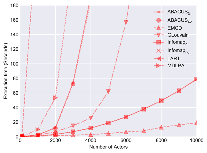
(a)

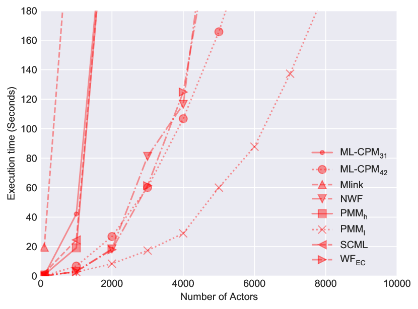
(b)

Figure 17: Scalability of different community detection methods with respect to the number of actors

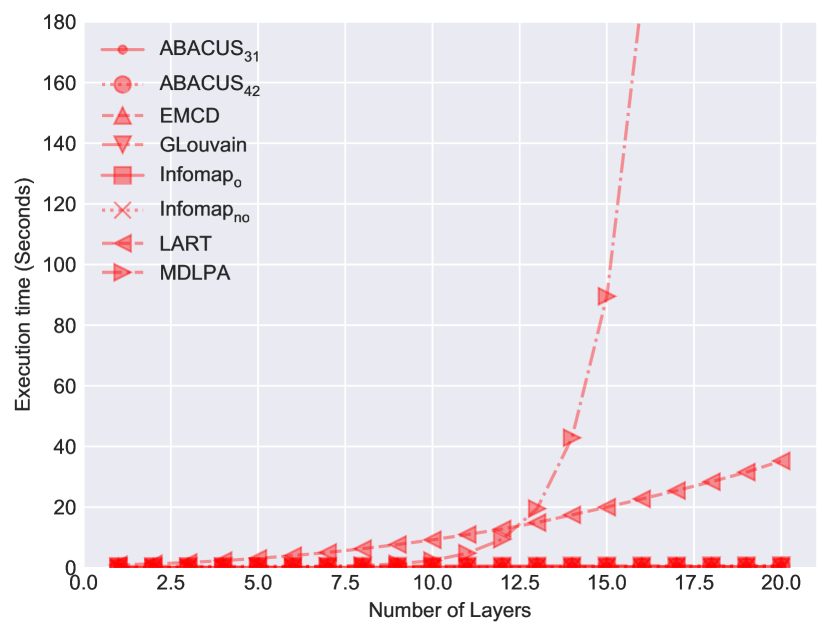
(a)

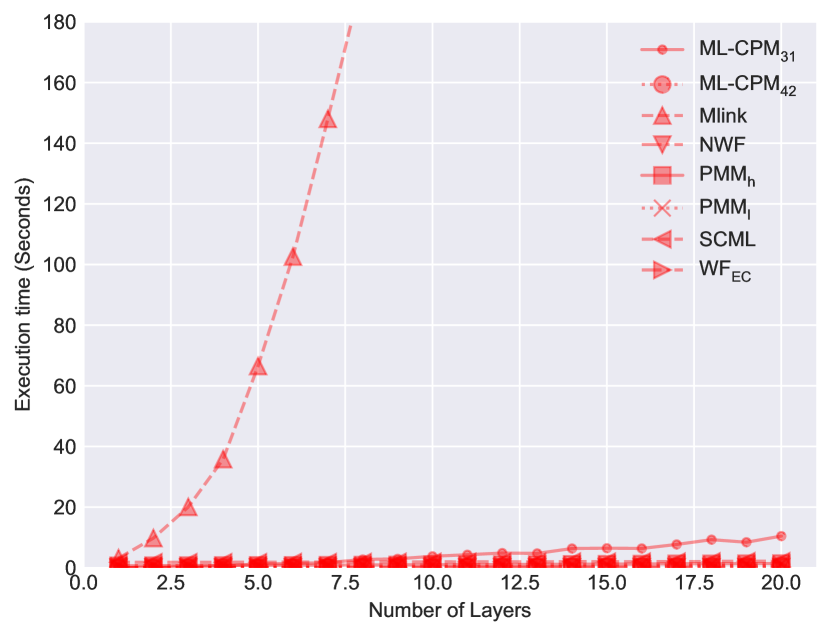
(b)

Figure 18: Scalability of different community detection methods with respect to the number of layers

6.1.5 Impact of noise

Figure 19 shows how the accuracy of the tested methods changes when we increase the number of edges across ground-truth communities. The basic data has been generated with 100 actors, 3 layers, 10 Pillar Equal Partitioning communities, and the $x$ axis indicates the probability of nodes in different communities to be adjacent. The results show how GLouvain with a high omega is less affected by noise than other methods, although this should be considered a result of the presence of pillar communities and the fact that high values of omega force the generation of pillars. Interestingly, Infomap shows a phase transition: with low noise it can identify the correct communities, then suddenly it starts returning one single community leading to an Omega Index value of 0.

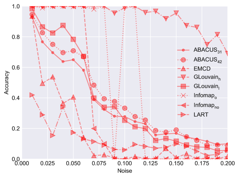
(a)

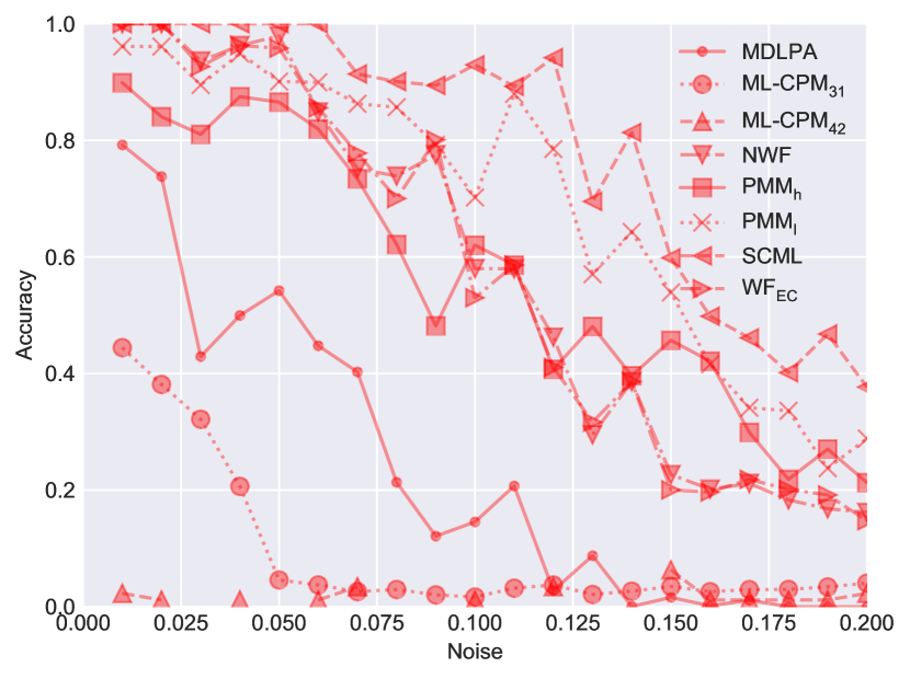
(b)

Figure 19: Impact of noise on accuracy

6.2 Local Methods

In this section we report the experimental results of the comparative evaluation of local multiplex community detection methods. The section is structured as follows: Section 6.2.1 presents the results of the accuracy analysis, Section 6.2.2 reports on the results of the pairwise comparison between different methods, while Section 6.2.3 discusses scalability issues.

6.2.1 Accuracy analysis

We performed an accuracy analysis on the local community detection methods, by comparing the local community of each actor to the one that same actor belongs to in the ground truth. Similarity is computed using the Jaccard index, while the final accuracy value is the average over all actors.

Figure  20 shows results on real-world networks. On AUCS, accuracy is in the range of $0.5$–$0.7$ for $4$ out of $5$ methods, with ML-LCD_(wlsim) being the best performer ($0.7$). Much lower accuracy values were obtained on DKPol, where the best performing method was ML-LCD_(lwsim) ($0.27$).

Concerning synthetic networks, we limited our analysis to networks with a pillar partitioning community structure (PEP and PNP), for compatibility with the methods’ output (both return actor communities). In these cases, we observed that accuracies are much higher than the ones observed for real-world networks, with all values in the range [$0.8$,$1.0$]. ML-LCD_(clsim) is the best performing method, since it is able to perfectly identify the ground truth community structure on both networks.

Summarizing, while all methods proved to be able to identify synthetic pillar community structures, their performance was much worse on real-world networks. These results confirm the behavior observed for global methods (cf. Section 6.1.2). Moreover, it should be pointed out that comparing a global community structure (i.e., the ground truth) to a set of local ones (i.e., the results obtained by local methods on all actors) may not be completely fair. The ground truth in this case represents a global partitioning of the network, while local communities are actor-centered, query dependent and, in general, they overlap with each other. Moreover, they may be discovered without having a complete knowledge of the network graph, which is the case for ML-LCD. Although based on the comparison of conceptually different objects (i.e., global and local communities), our accuracy analysis is still significant as it quantifies to what extent the local community formed around a certain actor falls inside the community found in the global structure that contains the actor. Unfortunately, no networks with an associated ground truth of multiplex local communities are available at the time of writing.

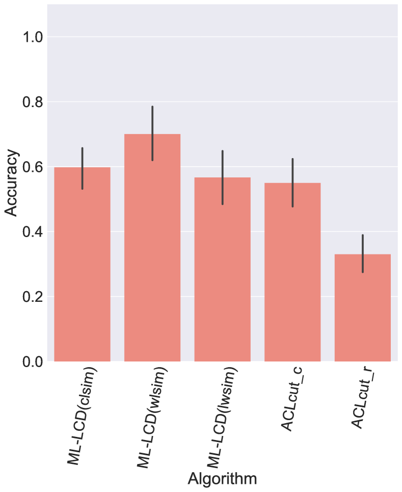
(a) AUCS

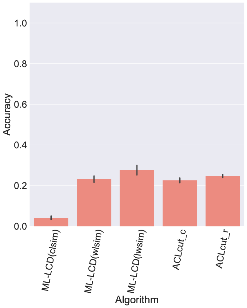
(b) DKPol

Figure 20: Average accuracy of the local methods with respect to a ground truth, on real-world networks

6.2.2 Pairwise comparison

As seen in Section 6.1.3 for global methods, we set up an equivalent evaluation stage based on pairwise comparison between the local methods. In this case, we resorted to the Jaccard index to measure the similarity of the community solutions produced by two local methods. Since these methods are query-dependent (i.e., they return the local community of a given query/seed node), we computed the Jaccard similarity between each pair of communities obtained using the same actor as seed, and then averaged the results over all actors.

Figure 21 reports on the results obtained on real-world networks. On most of these networks (DKPol, Airports, and Rattus), we can note that communities identified by different variants of ML-LCD and ACLcut tend to be very different. Looking at AUCS, the communities identified by all variants of both ML-LCD and ACLcut tend to be less different and a higher similarity can be observed among the three variants of ML-LCD.

For synthetic networks (Figure 22), it can be noted how similarities are higher for networks based on pillar community structures. In some cases (i.e., PEP and PNP) all methods are practically interchangeable, with all similarities equal or near to $1.0$. In other networks with pillar (i.e., PEO and PNO), semi-pillar (i.e., SEP and SEO) or both (MIX and HIE) community structures, similarities are stronger between the different variants of each method. Summing up, we observed some similarities in the behavior of all local methods on some real-world and synthetic networks, with an expected tendency of the variants of a same method to identify similar local communities. Nevertheless, this cannot be taken as a general rule, since we also observed specific cases where all methods behaved differently from each other, both on real-world and synthetic networks.

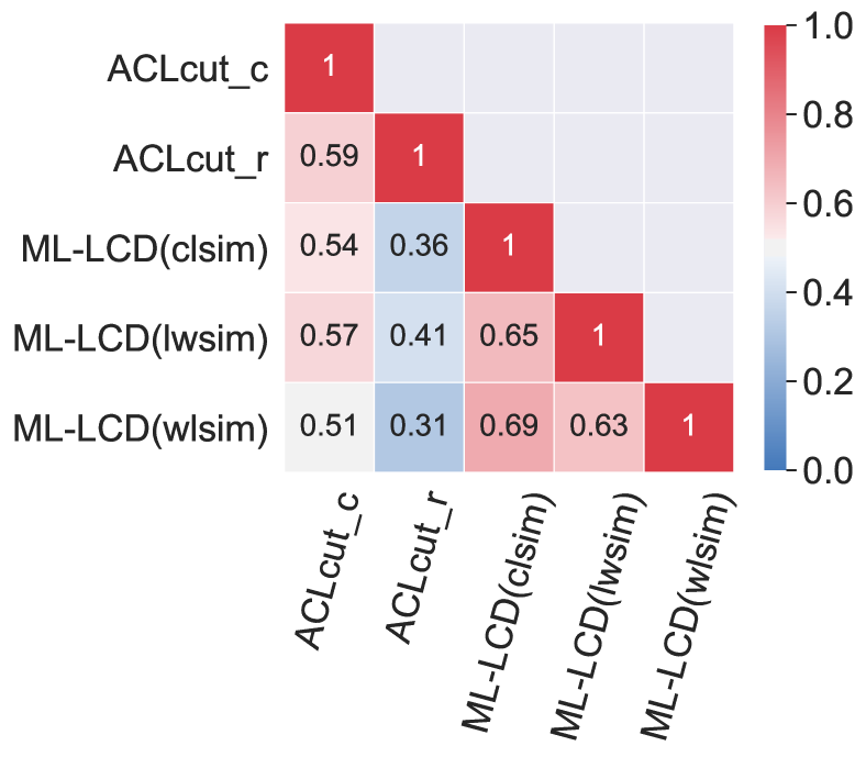
(a) AUCS

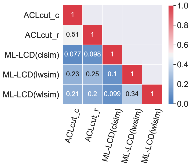
(b) DKPol

Figure 21: Average pairwise similarity among the different local methods on real-world networks

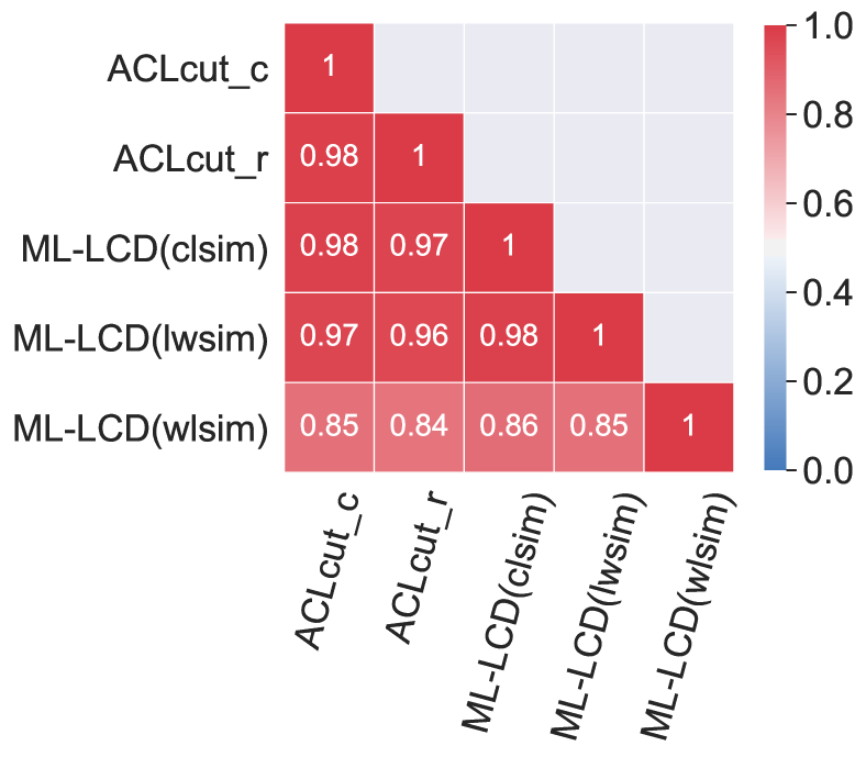
(a) PEP

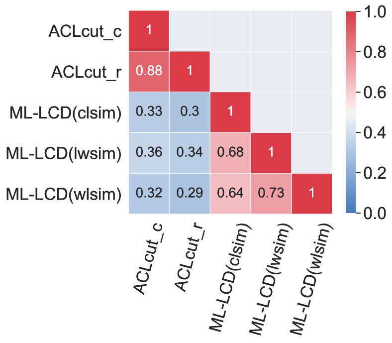
(b) PEO

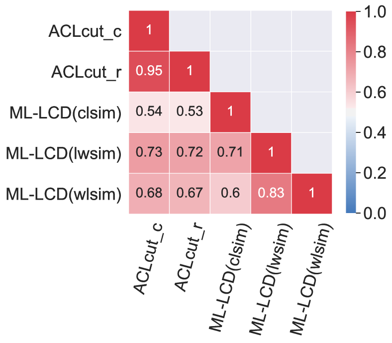
(c) HIE

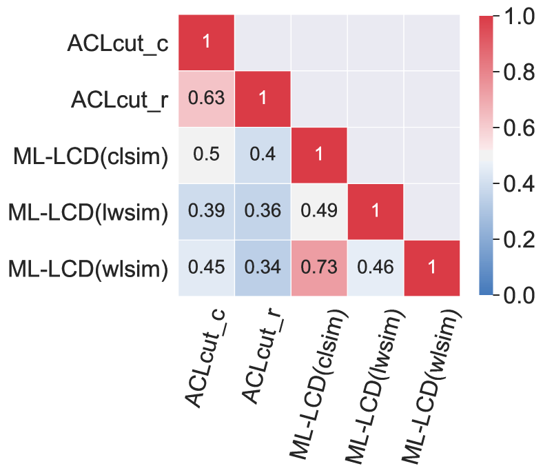
(d) MIX

Figure 22: Average pairwise similarity among the different local methods when the same seed is used as an input, on selected synthetic networks

Figures 23, 24 report the standard deviation of the average pairwise similarity among local methods on real-world datasets and synthetic datasets reported in Section 6.2.2.

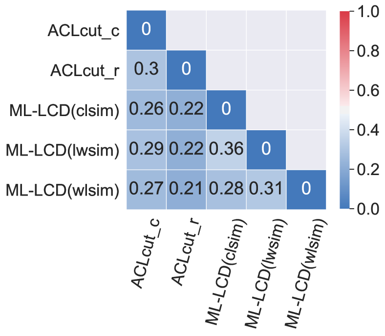
(a) AUCS

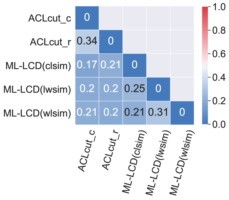
(b) DKPol

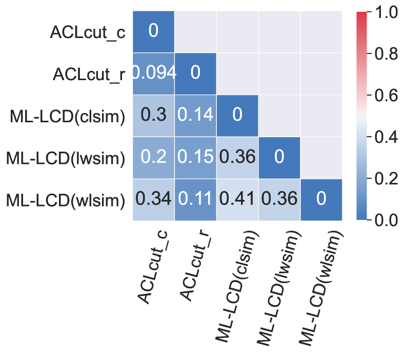
(c) Airports

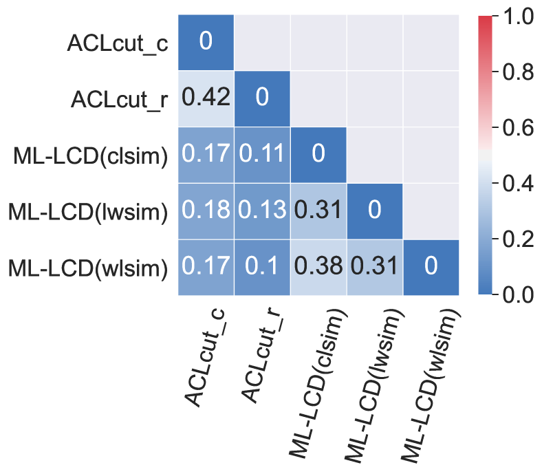
(d) Rattus

Figure 23: Standard deviation for average pairwise similarity among the different local methods (real networks)

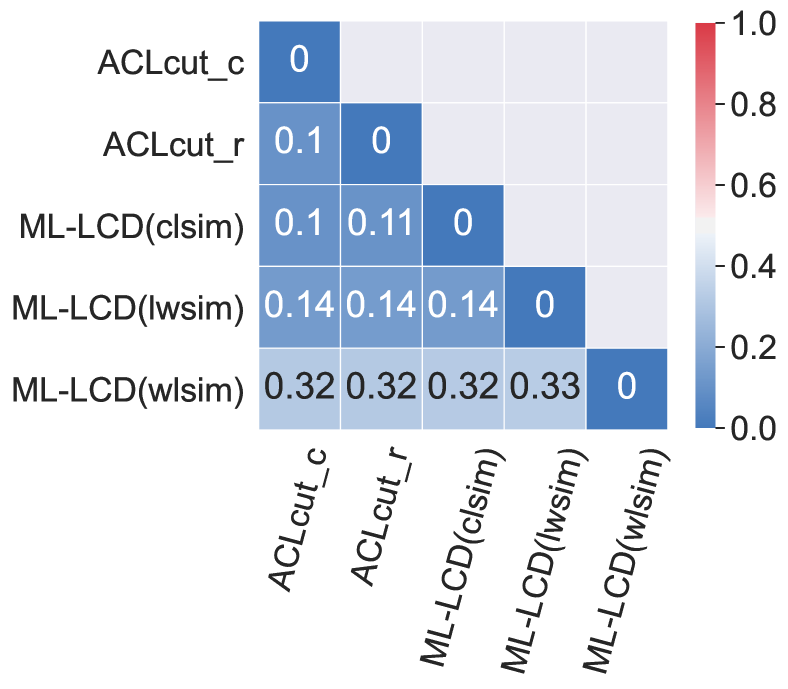
(a) PEP

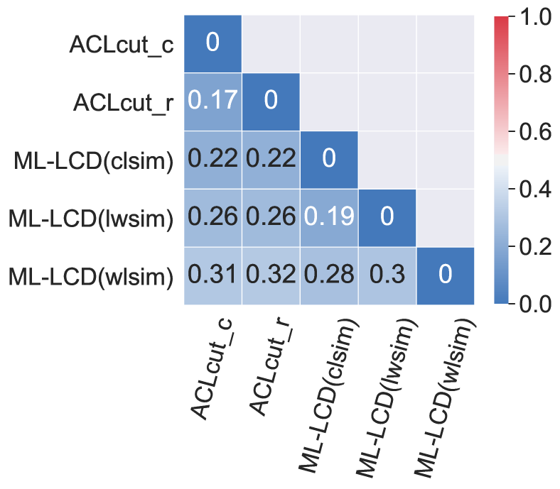
(b) PNP

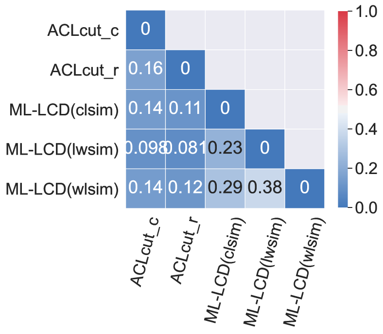
(c) PEO

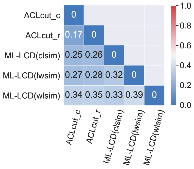
(d) PNO

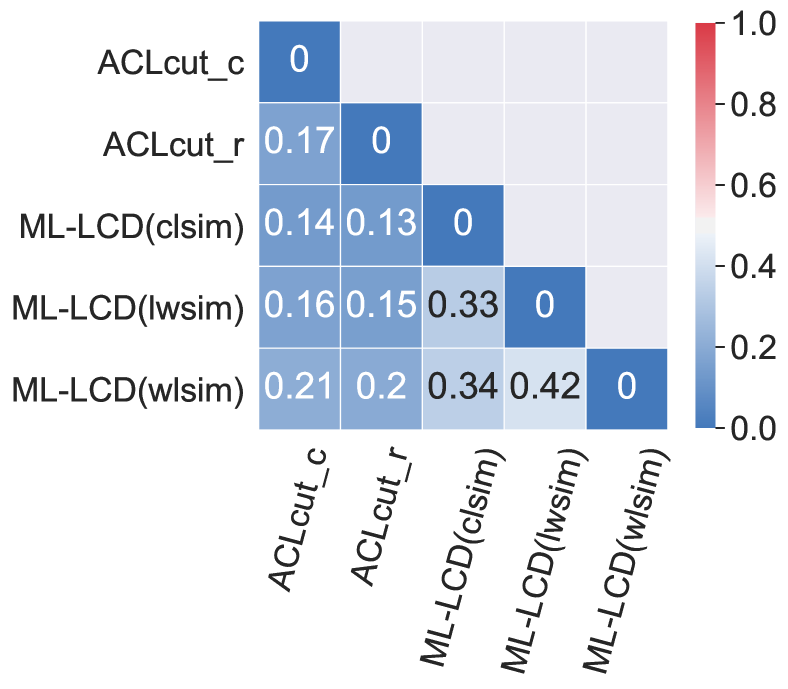
(e) SEP

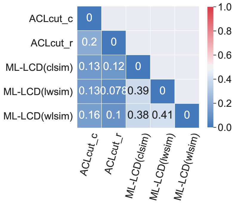
(f) SEO

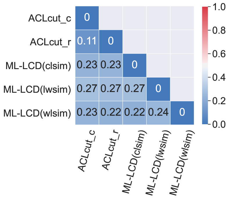
(g) NHN

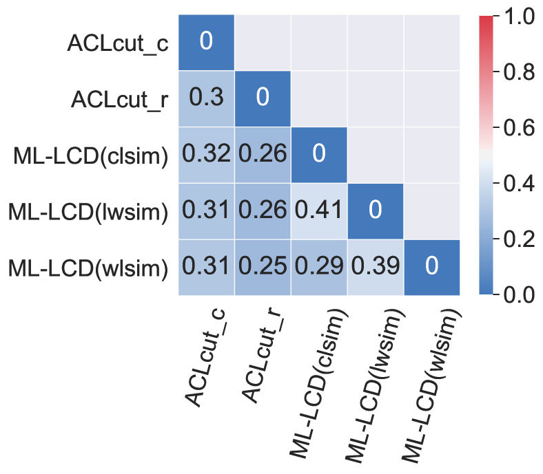
(h) NNM

Figure 24: Standard deviation for average pairwise similarity among the different local methods (synthetic networks)

6.2.3 Scalability Analysis

We tested the scalability of local community detection methods in terms of number of actors and number of layers. To carry out the experiment we used the synthetic networks already used for the global case (Section 6.1.4). For each network, we present median execution times obtained on 100 random seeds. For each method, we choose the least scalable variant as a representative of that method’s scalability.

Figures 25–26 show results related to scalability in terms of number of actors and of layers respectively. Both methods showed a similar good scalability, with ML-LCD showing a higher dispersion depending on the chosen seeds.

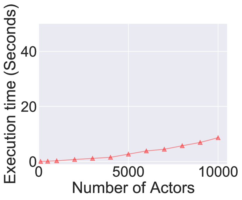
(a) ACLcut_c

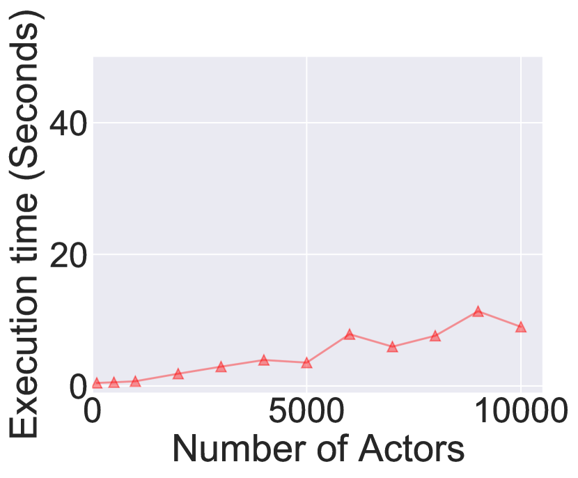
(b) ML-LCD_(clsim)

Figure 25: Median scalability of local methods with respect to the number of actors in the multiplex network

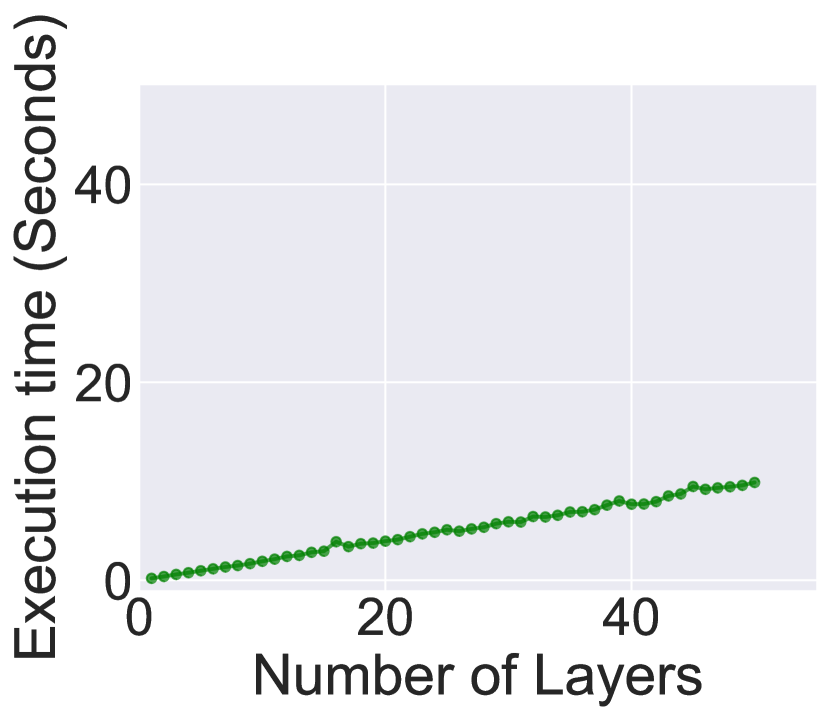
(a) ACLcut_c

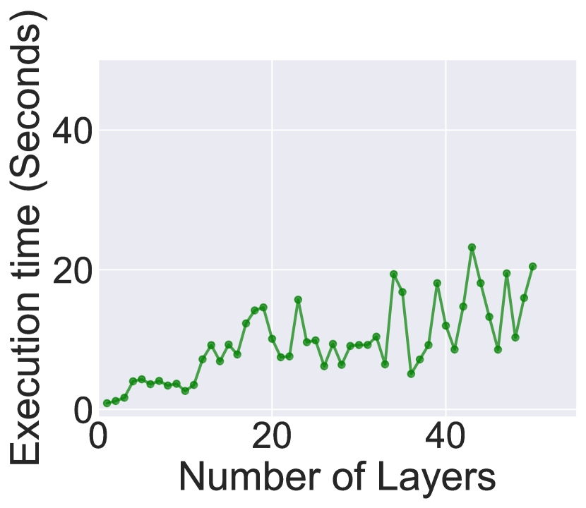
(b) ML-LCD_(clsim)

Figure 26: Median scalability of local methods with respect to the number of layers in the multiplex network

7 Discussion

Our experimental study had two main outcomes. First, it allowed us to identify guidelines about which methods can be the most appropriate for the data and the task at hand. Second, observing in which cases the reviewed methods consistently failed in identifying the expected communities allowed us to identify the multiplex community structures that are challenging with the currently available community detection algorithms. While the comparative evaluation of community detection methods is a complex process, and additional types of analysis should also be considered in the future, such as the approach used by [19] for single-layer methods, our work highlights a set of open problems for community detection methods in multiplex networks.

Accuracy analysis on synthetic networks has revealed that most of the methods perform very well when the community structure is made of disjoint pillars. Among the many well-performing methods, Infomap and SCML are consistently discovering community structures that are close or equal to the ground truth, GLouvain and the methods using Louvain are also performing well but have some issues with communities of varying size. whereas ML-LCD_(clsim) appears to be the best choice among the local methods. It is worth noticing that simpler flattening methods are also among the best methods.

With regard to non-pillar community structures, we have observed a considerable reduction in the achieved accuracy scores for almost all methods. This observation raises the following question: what kind of assumptions are considered by different methods when multiplex communities are identified? It is clear that there is a tendency, even if not always explicitly declared, to assume that multiplex communities are pillar communities expanding over all the layers of the multiplex network. For instance, multi-slice modularity [40] rewards pillar communities when calculating the modularity score, and spectral methods assume the existence of a latent community structure at actor level. While pillar community structures are perfectly reasonable and can be assumed to exist in many scenarios, they are also the simplest possible cases we tested in this article. As multiplex approaches have been developed to overcome the oversimplification of monoplex networks, relying on a single type of ideal community structure seems, at least, a missed opportunity. Thus, more work has to be done on improving the accuracy of community detection methods for non-pillar community structures.

A second set of considerations can be drawn by looking at the results obtained by the evaluated methods when applied to real-world datasets. Our experiments have shown that, on real-world datasets, the detected community structures largely differ from the ground truth. This raises two interesting questions. First, to which extent is the assumed ground truth itself a valid assumption? In other words, does the ground truth given for a real dataset always describe the community structures identified by a community detection method, or does it capture only one part of the whole picture? The answer to this question is never trivial even in monoplex networks. Nevertheless it is easy to see how adding more layers makes it further complicated. For example, both DKPol and AUCS ground truths group together individuals belonging to the same organization (political parties in one case and research groups in the other). The question then becomes whether it is reasonable to assume that the selected relations, observed in the multiplex networks, will produce a community structure corresponding to this formal grouping, and to some extent, how different relations (thus different layers) can be more or less aligned with the hypothesis described above. Will members of the same research group work together, or publish together? Have lunch and fun together? Will members of the same political party retweet each other on Twitter, and reply to each other? Indeed, looking at the accuracy of the community structures identified for the real world datasets, especially in the case of DKPol, one might ask whether we are observing a generalized failure of the community detection methods, or conversely, whether the community detection methods were actually able to observe relevant structures that were just different from the community structures assumed in the ground truth.

The second question, which is strongly related to the first one, is whether all the layers included in these datasets positively contribute to an accurate identification of the community structure in these datasets, or whether some of them add more noise that heavily affect the identification process. Indeed, the fact that most of the community detection methods always give an output, no matter what layers are included in the input multiplex network, makes the inclusion of more input layers potentially problematic. Layers, besides being defined by a specific internal topology, are also defined by internal logics that might or might not be coherent with those of the other layers. The DKPol dataset represents a good example of this problem. Some detailed analysis of the three layers composing the multiplex network has shown that retweets and following/follower interactions follow relatively assortative dynamics for political parties. The replies, however, are more frequent between members of different political parties. Here we think that more efforts have to be made in the modelling phase of the multiplex network and some layer-specific measures should be developed to lead the choice of the layers that contribute to the identification of the communities. Several such multilayer network simplification methods exist, and more can be developed, as reviewed in [25].

A separate consideration should be made about the similarities of the obtained results. Focusing, for the above-mentioned reason, mainly on the results obtained from the synthetic networks, it is possible to observe some general patterns. Global partitioning methods show a remarkable level of similarity in detecting community structures based on a pillar-like model. Semi-pillar and hierarchical community structures show a lower degree of similarity between the retrieved community structures. We should also consider that differences in the results of different algorithms may be partially due to the fact that some algorithms use heuristics to optimize an objective function (e.g., generalized Louvain), therefore they might not achieve the optimal value.

Local methods show a behavior that is, to some extent, similar to the global partitioning methods. When tested on pillar communities they show a remarkable similarity between the produced communities, which can easily lead to calling them interchangeable. Nevertheless, the less pillar-like the community structure in the data is, the higher the differences seem to be at first between ACLcut and ML-LCD and then also between different settings of the same algorithm.

Scalability analysis has also provided useful information about specific methods with scalability issues, which can be used to select feasible approaches depending on the data.

We would also like to draw additional remarks that might be considered mainly by practitioners. Community detection remains a challenging task, and further complicated in multilayer networks, which is testified by the plethora of available approaches and methods, most of which have been studied in our extensive survey, while new others are currently under development at the time of this writing. From a practical viewpoint, the core problems are, on the one hand, i) to select the most suited algorithm and parameterization for a target application domain, and on the other hand, ii) to have it clear in mind what kind of community we are interested in or we expect to detect. Problem i) should be addressed by taking into account that community detection methods, especially if belonging to different methodological approaches, will easily discover different patterns in a multilayer network, mainly because every method has its own bias resulting from the optimization of different criteria. We believe this variety of choice should not be seen as a negative point, but rather as an opportunity to find out communities with different structures and related meanings. Also, if the need for having a unified solution from different available ones still remains as a priority, the ensemble-based consensus approach could be considered as the way to go. Understanding problem ii) will nonetheless be crucial in most cases, as it may pose a requirement for the structure of the communities to be discovered, thus possibly impacting on the choice of the method to be used. In any case, this will also depend on the actual presence of communities of a desired form in the input network; for instance, any method based on the identification of cliques of a given size will likely fail if such cliques are rare or missing at all in the input network. Therefore, one suggestion in this regard would be to deepen as much as possible the study of structural micro/mesoscopic characteristics of the input network, both in its entirety as a complex system and at the level of its constituent layers, to better prepare the subsequent analysis for the community detection task.

Despite the complexity of the multiplex community detection task emerging from our study, we would like to conclude our discussion on a positive note. There are many cases where we have a good expectation of what type of community structures could be found in the data. One example is the simple case of actor communities that expand over multiple layers, as in the AUCS network where people inside the same research group work together, publish papers together and go to lunch together – although the multilayer data allows us to appreciate how administrative people are part of the community only on some layers, and not for example of the co-authorship one. Another example are hierarchical communities where the layers represent different organizational levels, e.g., University-level interactions, Department-level interactions, research-group-level interactions, etc. Overlapping can also be expected inside data describing flexible organizations with people having multiple roles. These examples share the same features of some of our synthetic networks (Pillar, Hierarchical, Overlapping). Therefore, domain knowledge about what type of communities to expect can be used together with our accuracy (and scalability, in case of larger networks) plots to determine which algorithms to prioritize.

8 Concluding remarks

This work has highlighted some facts. When the community structure is simple (pillar, non overlapping communities of similar size) we can expect most of the reviewed methods to work well. Therefore, scalability considerations may be used to choose the best algorithm. When we depart from this simple type of communities it becomes more difficult to identify them, and the concept of type of community structure itself requires more research. We can however see how some more sophisticated approaches not relying on flattening can be more successful in specific cases. Given the different types of communities identified by different methods, it can be valuable to try multiple approaches while exploring multiplex network data. The difficulty to handle some of the data suggests that more research in network preprocessing would be valuable [25] in addition to the development of new community detection methods. Community detection in multiplex networks is an active area, and it will be interesting to see how new algorithms address the challenges highlighted in this work. The code used for the experiments is available at https://bitbucket.org/uuinfolab/20csur and can be extended to include additional methods and data.

References

- [1] Nazanin Afsarmanesh and Matteo Magnani. Finding overlapping communities in multiplex networks. In Proceedings of the 2018 International Conference on Social Informatics (SocInfo), 2018.
- [2] Michael J. Barber. Modularity and community detection in bipartite networks. Physical Review E, 76:066102, 2007.
- [3] Michele Berlingerio, Michele Coscia, and Fosca Giannotti. Finding and characterizing communities in multidimensional networks. In International Conference on Advances in Social Networks Analysis and Mining (ASONAM), pages 490–494. IEEE Computer Society Washington, DC, USA, 2011.
- [4] Michele Berlingerio, Fabio Pinelli, and Francesco Calabrese. ABACUS: frequent pAttern mining-BAsed Community discovery in mUltidimensional networkS. Data Mining and Knowledge Discovery, 27(3):294–320, 2013.
- [5] Brigitte Boden, Stephan Günnemann, Holger Hoffmann, and Thomas Seidl. Mining coherent subgraphs in multi-layer graphs with edge labels. In Proceedings of the 18th ACM SIGKDD international conference on Knowledge discovery and data mining - KDD ’12, page 1258. ACM Press, aug 2012.
- [6] Cecile Bothorel, Juan David Cruz, Matteo Magnani, and Barbora Micenkova. Clustering attributed graphs: models, measures and methods. Network Science, 3(3):408–444, 2015.
- [7] Oualid Boutemine and Mohamed Bouguessa. Mining Community Structures in Multidimensional Networks. ACM Transactions on Knowledge Discovery from Data, 11(4):1–36, jun 2017.
- [8] Piotr Bródka, Anna Chmiel, Matteo Magnani, and Giancarlo Ragozini. Quantifying layer similarity in multiplex networks: A systematic study. Royal Society Open Science, 2018.
- [9] Piotr Bródka, Tomasz Filipowski, and Przemysław Kazienko. An Introduction to Community Detection in Multi-layered Social Network. In Information Systems, E-learning, and Knowledge Management Research, Communications in Computer and Information Science, pages 185–190. Springer, Berlin, Heidelberg, 2013.
- [10] Piotr Bródka, Krzysztof Skibicki, Przemyslaw Kazienko, and Katarzyna Musial. A degree centrality in multi-layered social network. In International Conference on Computational Aspects of Social Networks (CASoN), pages 237–242. IEEE, oct 2011.
- [11] Alessio Cardillo, Jesús Gómez-Gardeñes, Massimiliano Zanin, Miguel Romance, David Papo, Francisco del Pozo, and Stefano Boccaletti. Emergence of network features from multiplexity. Scientific Reports, 2013.
- [12] Jiyang Chen, Osmar R. Zaïane, and Randy Goebel. Local community identification in social networks. In 2009 International Conference on Advances in Social Network Analysis and Mining, ASONAM, pages 237–242, 2009.
- [13] Linda M. Collins and Clyde W. Dent. Omega: A General Formulation of the Rand Index of Cluster Recovery Suitable for Non-disjoint Solutions. Multivariate Behavioral Research, 23(2):231–242, apr 1988.
- [14] Manlio De Domenico, Andrea Lancichinetti, Alex Arenas, and Martin Rosvall. Identifying modular flows on multilayer networks reveals highly overlapping organization in interconnected systems. Phys. Rev. X, 5:011027, Mar 2015.
- [15] Manlio De Domenico, Vincenzo Nicosia, Alexandre Arenas, and Vito Latora. ARTICLE Structural reducibility of multilayer networks. Nature Communications, 6, 2015.
- [16] Mark E. Dickison, Matteo Magnani, and Luca Rossi. Multilayer Social Networks. Cambridge University Press, 2016.
- [17] Xiaowen Dong, Pascal Frossard, Pierre Vandergheynst, and Nikolai Nefedov. Clustering on Multi-Layer Graphs via Subspace Analysis on Grassmann Manifolds. IEEE Transactions on Signal Processing, 62(4):905–918, feb 2014.
- [18] Daniel Edler, Ludvig Bohlin, and Martin Rosvall. Mapping higher-order network flows in memory and multilayer networks with infomap. CoRR, abs/1706.04792, 2017.
- [19] Amir Ghasemian, Homa Hosseinmardi, and Aaron Clauset. Evaluating Overfit and Underfit in Models of Network Community Structure. IEEE Transactions on Knowledge and Data Engineering, pages 1–1, 2019.
- [20] Roger Guimera, Marta Sales-Pardo, and Luis A. Nunes Amaral. Module identification in bipartite and directed networks. Physical Review E, 76:036102, 2007.
- [21] Obaida Hanteer and Matteo Magnani. Unspoken Assumptions in Multi-layer Modularity maximization. Scientific Reports, 10(1):11053, 2020.
- [22] Obaida Hanteer and Luca Rossi. The meaning of dissimilar: An evaluation of various similarity quantification approaches used to evaluate community detection solutions. In Proceedings of the IEEE/ACM International Conference on Advances in Social Networks Analysis and Mining, pages 513–518, Vancouver, Canada, 2019.
- [23] Obaida Hanteer, Luca Rossi, Davide Vega D’Aurelio, and Matteo Magnani. From Interaction to Participation: The Role of the Imagined Audience in Social Media Community Detection and an Application to Political Communication on Twitter. In Ulrik Brandes, Chandan Reddy, and Andrea Tagarelli, editors, IEEE/ACM International Conference on Advances in Social Networks Analysis and Mining, ASONAM, pages 531–534. {IEEE} Computer Society, 2018.
- [24] Xinyu Huang, Dongming Chen, Tao Ren, and Dongqi Wang. A survey of community detection methods in multilayer networks. Data Mining and Knowledge Discovery, pages 1–45, oct 2020.
- [25] Roberto Interdonato, Matteo Magnani, Diego Perna, Andrea Tagarelli, and Davide Vega. Multilayer network simplification: Approaches, models and methods. Comput. Sci. Rev., 36:100246, 2020.
- [26] Roberto Interdonato, Andrea Tagarelli, Dino Ienco, Arnaud Sallaberry, and Pascal Poncelet. Node-Centric Community Detection in Multilayer Networks with Layer-Coverage Diversification Bias. In Proceedings of the 8th Conference on Complex Networks (CompleNet 2017), pages 57–66. Springer International Publishing, 2017.
- [27] Lucas G. S. Jeub, Michael W. Mahoney, Peter J. Mucha, and Mason A. Porter. A local perspective on community structure in multilayer networks. Network Science, 5(2):144–163, 2017.
- [28] Inderjit S Jutla, Lucas G S Jeub, and Peter J Mucha. A generalized Louvain method for community detection implemented in Matlab. Technical report, 2011-2017.
- [29] Jungeun Kim and Jae-Gil Lee. Community Detection in Multi-Layer Graphs. ACM SIGMOD Record, pages 37–48, 2015.
- [30] Jungeun Kim, Jae-gil Lee, and Sungsu Lim. Differential Flattening: A Novel Framework for Community Detection in Multi-Layer Graphs. ACM Transactions on Intelligent Systems and Technology (TIST), 8(2):27, 2016.
- [31] Mikko Kivelä, Alexandre Arenas, Marc Barthelemy, James P. Gleeson, Yamir Moreno, and Mason A. Porter. Multilayer Networks. Journal of Complex Networks, 2(3):203–271, sep 2014.
- [32] Zhana Kuncheva and Giovanni Montana. Community Detection in Multiplex Networks using Locally Adaptive Random Walks. In Proceedings of the IEEE/ACM International Conference on Advances in Social Networks Analysis and Mining, ASONAM, pages 1308–1315. ACM Press, 2015.
- [33] Andrea Lancichinetti and Santo Fortunato. Consensus Clustering in Complex Networks. Scientific Reports, 2(336), 2012.
- [34] Huajing Li, Zaiqing Nie, Wang-Chien Lee, Lee Giles, and Ji-Rong Wen. Scalable community discovery on textual data with relations. In Proceedings of the 17th ACM Conference on Information and Knowledge Management, CIKM ’08, pages 1203–1212, New York, NY, USA, 2008. ACM.
- [35] Yixuan Li, Kun He, David Bindel, and John E. Hopcroft. Uncovering the small community structure in large networks: A local spectral approach. In Proc. of the 24th International Conference on World Wide Web, WWW 2015, Florence, Italy, May 18-22, 2015, pages 658–668, 2015.
- [36] Chuan Wen Loe and Henrik Jeldtoft Jensen. Comparison of communities detection algorithms for multiplex. Physica A: Statistical Mechanics and its Applications, 431:29–45, 2015.
- [37] Lijia Ma, Maoguo Gong, Jianan Yan, Wenfeng Liu, and Shanfeng Wang. Detecting composite communities in multiplex networks: A multilevel memetic algorithm. Swarm and Evolutionary Computation, 39:177–191, apr 2018.
- [38] Matteo Magnani and Luca Rossi. The ML-model for multi-layer social networks. In Proceedings - 2011 International Conference on Advances in Social Networks Analysis and Mining, ASONAM 2011, 2011.
- [39] Raul J. Mondragon, Jacopo Iacovacci, and Ginestra Bianconi. Multilink communities of multiplex networks. PLOS ONE, 13(3):e0193821, mar 2018.
- [40] Peter J. Mucha and Mason A. Porter. Communities in multislice voting networks. Chaos: An Interdisciplinary Journal of Nonlinear Science, 20(4), 2010.
- [41] Peter J Mucha, Thomas Richardson, Kevin Macon, Mason A Porter, and Jukka-Pekka Onnela. Community structure in time-dependent, multiscale, and multiplex networks. Science (New York, N.Y.), 328(5980):876–8, may 2010.
- [42] Gabriel Murray, Giuseppe Carenini, and Raymond Ng. Using the omega index for evaluating abstractive community detection. In Proceedings of Workshop on Evaluation Metrics and System Comparison for Automatic Summarization, pages 10–18. Association for Computational Linguistics, 2012.
- [43] Leto Peel, Daniel B. Larremore, and Aaron Clauset. The ground truth about metadata and community detection in networks. Science Advances, 3(5):e1602548, may 2017.
- [44] Clara Pizzuti and Annalisa Socievole. Many-objective optimization for community detection in multi-layer networks. In 2017 IEEE Congress on Evolutionary Computation (CEC), pages 411–418. IEEE, jun 2017.
- [45] Guo-Jun Qi, Charu C. Aggarwal, and Thomas Huang. Community detection with edge content in social media networks. In 2012 IEEE 28th International Conference on Data Engineering (ICDE), volume 00, pages 534–545, 04 2012.
- [46] Luca Rossi and Matteo Magnani. Towards effective visual analytics on multiplex and multilayer networks. Chaos, Solitons and Fractals, 72, 2015.
- [47] Yiye Ruan, David Fuhry, and Srinivasan Parthasarathy. Efficient Community Detection in Large Networks using Content and Links. 2012.
- [48] Arlei Silva, Wagner Meira, Jr., and Mohammed J. Zaki. Mining attribute-structure correlated patterns in large attributed graphs. Proc. VLDB Endow., 5(5):466–477, January 2012.
- [49] Yizhou Sun and Jiawei Han. Mining heterogeneous information networks: a structural analysis approach. ACM SIGKDD Explorations Newsletter, 14(2):20–28, 2013.
- [50] Yizhou Sun, Jiawei Han, Peixiang Zhao, Zhijun Yin, Hong Cheng, and Tianyi Wu. RankClus: integrating clustering with ranking for heterogeneous information network analysis. In International Conference on Extending Database Technology (EDBT), pages 565–576. ACM Press, 2009.
- [51] Yizhou Sun, Yintao Yu, and Jiawei Han. Ranking-based clustering of heterogeneous information networks with star network schema. In Proceedings of the 15th ACM SIGKDD international conference on Knowledge discovery and data mining - KDD ’09, page 797. ACM Press, 2009.
- [52] Andrea Tagarelli, Alessia Amelio, and Francesco Gullo. Ensemble-based community detection in multilayer networks. Data Mining and Knowledge Discovery, 31(5):1506–1543, Sep 2017.
- [53] Lei Tang and Huan Liu. Community Detection and Mining in Social Media. Synthesis Lectures on Data Management. Morgan & Claypool Publishers, 2010.
- [54] Lei Tang, Xufei Wang, and Huan Liu. Uncoverning groups via heterogeneous interaction analysis. 2009 Ninth IEEE International Conference on Data Mining, pages 503–512, 2009.
- [55] Lei Tang, Xufei Wang, and Huan Liu. Community detection via heterogeneous interaction analysis. Data Mining and Knowledge Discovery, 25(1):1–33, jul 2012.
- [56] Zhiqiang Xu, Yiping Ke, Yi Wang, Hong Cheng, and James Cheng. A model-based approach to attributed graph clustering. In Proceedings of the 2012 ACM SIGMOD International Conference on Management of Data, SIGMOD ’12, pages 505–516, New York, NY, USA, 2012. ACM.
- [57] Xuemeng Zhai, Wanlei Zhou, Gaolei Fei, Weiyi Liu, Zhoujun Xu, Chengbo Jiao, Cai Lu, and Guangmin Hu. Null Model and Community Structure in Multiplex Networks. Scientific Reports, 8(1):3245, dec 2018.
- [58] Yang Zhou, Hong Cheng, and Jeffrey Xu Yu. Graph clustering based on structural/attribute similarities. Proc. VLDB Endow., 2(1):718–729, 2009.
- [59] Yang Zhou and Ling Liu. Social influence based clustering of heterogeneous information networks. ACM SIGKDD international conference on Knowledge discovery and data mining, page 338, 2013.