Abstract

It is difficult to predict how antibodies will behave when mixed together, even after each has been independently characterized. Here, we present a statistical mechanical model for the activity of antibody mixtures that accounts for whether pairs of antibodies bind to distinct or overlapping epitopes. This model requires measuring $n$ individual antibodies and their $\frac{n(n-1)}{2}$ pairwise interactions to predict the $2^{n}$ potential combinations. We apply this model to epidermal growth factor receptor (EGFR) antibodies and find that the activity of antibody mixtures can be predicted without positing synergy at the molecular level. In addition, we demonstrate how the model can be used in reverse, where straightforward experiments measuring the activity of antibody mixtures can be used to infer the molecular interactions between antibodies. Lastly, we generalize this model to analyze engineered multidomain antibodies, where components of different antibodies are tethered together to form novel amalgams, and characterize how well it predicts recently designed influenza antibodies.

Author summary

With the rise of new combination antibody therapeutic regimens, it is important to understand how antibodies work together as well as individually. Here, we investigate the specific case of monoclonal antibodies targeting a cancer-causing receptor or the influenza virus and develop a statistical mechanical framework that predicts the effectiveness of a mixture of antibodies. The power of this model lies in its ability to make a large number of predictions based on a limited amount of data. For example, once 10 antibodies have been individually characterized, our model can predict how any of the $2^{10}=1024$ combinations will behave. This predictive power provides ample opportunities to test our model and paves the way to expedite the design of future therapeutics.

Introduction

Antibodies can bind with strong affinity and exquisite specificity to a multitude of antigens. Due to their clinical and commercial success, antibodies are one of the largest and fastest growing classes of therapeutic drugs [1]. While most therapies currently use monoclonal antibodies (mAbs), mounting evidence suggests that mixtures of antibodies can behave in fundamentally different ways [2]. There is ample precedent for the idea that combinations of therapeutics can be extremely powerful—for instance, during the past 50 years the monumental triumphs of combination anti-retroviral therapy and chemotherapy cocktails have provided unprecedented control over HIV and multiple types of cancer [3, 4], and in many cases no single drug has emerged with comparable effects. However, it is difficult to predict how antibody mixtures will behave relative to their constitutive parts. Often, the vast number of potential combinations is prohibitively large to systematically test, since both the composition of the mixture and the relative concentration of each component can influence its efficacy [5].

Here, we develop a statistical mechanical model that bridges the gap between how an antibody operates on its own and how it behaves in concert. Specifically, each antibody is characterized by its binding affinity and potency, while its interaction with other antibodies is described by whether its epitope is distinct from or overlaps with theirs. This information enables us to translate the molecular details of how each antibody acts individually into the macroscopic readout of a system’s activity in the presence of an arbitrary mixture.

To test the predictive power of our framework, we apply it to a beautiful recent case study of inhibitory antibodies against the epidermal growth factor receptor (EGFR), where 10 antibodies were individually characterized for their ability to inhibit receptor activity and then all possible 2-Ab and 3-Ab mixtures were similarly tested [6]. We demonstrate that our framework can accurately predict the activity of these mixtures based solely on the behaviors of the ten monoclonal antibody as well as their epitope mappings.

Lastly, we generalize our model to predict the potency of engineered multidomain antibodies from their individual components. Specifically, we consider the recent work by Laursen et al. where four single-domain antibodies were assayed for their ability to neutralize a panel of influenza strains, and then the potency of constructs comprising 2-4 of these single-domain antibodies were measured [7]. Our generalized model can once again predict the efficacy of the multidomain constructs based upon their constitutive components, once a single fit parameter is inferred to quantify the effects of the linker joining the single-domain antibodies. This enables us to quantitatively ascertain how tethering antibodies enhances the two key features of potency and breadth that are instrumental for designing novel anti-viral therapeutics. Notably, our models do not posit complex molecular synergy between antibodies. Our results therefore show that many antibody mixtures function without synergy, and hence that their effects can be computationally predicted to expedite future experiments.

Results

Modeling the mechanisms of action for antibody mixtures

Consider a monoclonal antibody that binds to a receptor and inhibits its activity. Two parameters characterize this inhibition: (1) the dissociation constant $K_{D}$ quantifies an antibody’s binding affinity (with a smaller value indicating tighter binding) and (2) the potency $\alpha$ relates the activity when an antibody is bound to the activity in the absence of antibody. A value of $\alpha=1$ represents an impotent antibody that does not affect activity while $\alpha=0$ implies that an antibody fully inhibits activity upon binding. As derived in S1 Text Section A, for an antibody that binds to a single site on a receptor, the activity at a concentration $c$ of antibody is given by

$$\text{Fractional Activity}=\frac{1+\alpha\frac{c}{K_{D}}}{1+\frac{c}{K_{D}}}.$$ (1)

To characterize a mixture of two antibodies, we not only need their individual dissociation constants and potencies but also require a model for how these antibodies interact. When two antibodies bind to distinct epitopes, the simplest scenario is that their ability to bind and inhibit activity is independent of the presence of the other antibody, and hence that their combined potency when simultaneously bound equals the product of their individual potencies (Fig 1A). Alternatively, if the two antibodies compete for the same epitope, they cannot both be simultaneously bound (Fig 1B).

We also define the general case of a synergistic interaction where the binding of the first antibody alters the binding or potency of the second antibody (Fig 1C, purple text). This definition encompasses cases where the second antibody binds more tightly ($K_{D,\text{eff}}^{(2)}<K_{D}^{(2)}$) or more weakly ($K_{D,\text{eff}}^{(2)}>K_{D}^{(2)}$) in the presence of the first antibody, as well as when the potency of the second antibody may increase ($\alpha_{2,\text{eff}}>\alpha_{2}$) or decrease ($\alpha_{2,\text{eff}}<\alpha_{2}$). This also includes cases where two epitopes slightly overlap and partially inhibit one another’s binding, and the competitive binding model can be viewed as the extreme limit $K_{D,\text{eff}}^{(2)}\to\infty$ where one antibody infinitely penalizes the binding of the other.

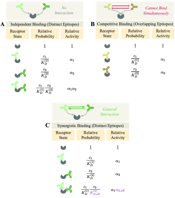
Figure 1: Binding modes for a 2-Ab mixture. Two antibodies with concentrations $c_{1}$ and $c_{2}$ can bind (A) independently to different epitopes or (B) competitively to the same epitope. (C) Antibodies bind synergistically if either the product of binding affinities ($K_{D}^{(j)}$) or potencies ($\alpha_{j}$) are altered when both antibodies bind.

While the synergistic model in Fig 1C has the merit of being highly general, an important feature of the independent and competitive models (Fig 1A,B) is that they predict all antibody combinations with few parameters. In both of these latter models, once the $K_{D}^{(j)}$ and $\alpha_{j}$ of 10 antibodies are known (which requires $2\cdot 10$ experiments) and their epitopes are mapped ($\frac{10\cdot 9}{2}$ additional experiments), the potency of all $2^{10}=1024$ possible mixtures of these antibodies can be predicted without recourse to fitting. In contrast, because the synergistic model allows arbitrary interactions between each combination of antibodies, the behavior of a mixture exhibiting synergy cannot be predicted without actually making a measurement on that combination to quantify the synergy.

For these reasons, in this work we focus on the two cases of independent or competitive binding and show how we can combine both models to transform our molecular understanding of each monoclonal antibody’s action into a prediction of the efficacy of an antibody mixture. Deviations from our predictions provide a rigorous way to measure antibody synergy by computing $\frac{K_{D,\text{eff}}^{(2)}}{K_{D}^{(2)}}$ and $\frac{\alpha_{2,\text{eff}}}{\alpha_{2}}$.

To mathematize the independent and competitive binding models, we enumerate the possible binding states and compute their relative Boltzmann weights. The fractional activity of each state equals the product of its relative probability and relative activity divided by the sum of all relative probabilities for normalization (see S1 Text Section A). When two antibodies bind independently as in Fig 1A, this factors into the form

$$\text{Fractional Activity}_{\text{(distinct epitopes)}}=\left(\frac{1+\alpha_{1}\frac{c_{1}}{K_{D}^{(1)}}}{1+\frac{c_{1}}{K_{D}^{(1)}}}\right)\left(\frac{1+\alpha_{2}\frac{c_{2}}{K_{D}^{(2)}}}{1+\frac{c_{2}}{K_{D}^{(2)}}}\right).$$ (2)

If these two antibodies compete for the same epitope as in Fig 1B, the activity becomes

$$\text{Fractional Activity}_{\text{(overlapping epitopes)}}=\frac{1+\alpha_{1}\frac{c_{1}}{K_{D}^{(1)}}+\alpha_{2}\frac{c_{2}}{K_{D}^{(2)}}}{1+\frac{c_{1}}{K_{D}^{(1)}}+\frac{c_{2}}{K_{D}^{(2)}}}.$$ (3)

These equations are readily extended to mixtures with three or more antibodies (see S1 Text Section A).

Antibody mixtures against EGFR are well characterized using independent and competitive binding models

To test the predictive power of the independent and competitive binding models, we applied them to published experiments on the epidermal growth factor receptor (EGFR) where ten monoclonal antibodies were individually characterized and then the activity of all 165 possible 2-Ab and 3-Ab mixtures was measured [6]. We first use each monoclonal antibody’s response to infer its dissociation constant $K_{D}$ and potency $\alpha$. We then utilize surface plasmon resonance (SPR) measurements to determine which pairs of antibodies bind independently and which compete for the same epitope. These data enable us to use the above framework and predict EGFR activity in the presence of any mixture.

EGFR is a transmembrane protein that activates in the presence of epidermal growth factors. Upon ligand binding, the receptor’s intracellular tyrosine kinase domain autophosphorylates which leads to downstream signaling cascades central to cell migration and proliferation. Overexpression of EGFR has been linked to a number of cancers, and decreasing EGFR activity in such tumors by sterically occluding ligand binding has reduced the rate of cancer proliferation [6].

Koefoed et al. investigated how a panel of ten monoclonal antibodies inhibit EGFR activity in the human cell line A431NS [6]. They then measured how 1:1 mixtures of two antibodies or 1:1:1 mixtures of three antibodies affect EGFR activity. All measurement were carried out at a total concentration of $2\frac{\mu\text{g}}{\text{mL}}$, implying that each antibody was half as dilute in the 2-Ab mixtures and one-third as dilute in the 3-Ab mixtures relative to the monoclonal antibody measurement.

The 45 possible 2-Ab mixtures (35 binding to distinct epitopes; 10 binding to overlapping epitopes) and the 120 possible 3-Ab mixtures (50 binding to distinct epitopes; 70 binding to overlapping epitopes) were assayed for their ability to inhibit EGFR activity. Fig 2A shows the experimental measurements for mixtures of two antibodies, with the monoclonal antibody measurements shown on the diagonal, the measured activity of 2-Ab mixtures shown on the bottom-left and the predicted activity on the top-right. Each antibody is labeled with its binding epitopes inferred through SPR [6], so that antibodies binding to overlapping epitopes are predicted using Eq (3) (pairs within the dashed gray boxes) while mixtures binding to distinct epitopes use Eq (2).

For example, antibodies #1 and #4 bind to distinct epitopes (III/C and III/B, respectively). Hence, the predicted activity of their mixture (0.50) very nearly equals the product of their individual activity ($0.65\times 0.75=0.49$), with the slight deviation arising because each antibody concentration was halved in the mixture ($c_{1}=c_{2}=1\frac{\mu\text{g}}{\text{mL}}$ for the 2-Ab mixture characterized by Eq (2), whereas the individual mAbs were measured at $c=2\frac{\mu\text{g}}{\text{mL}}$ using Eq (1)). The predicted activity roughly approximates the measured value 0.43 of the mixture.

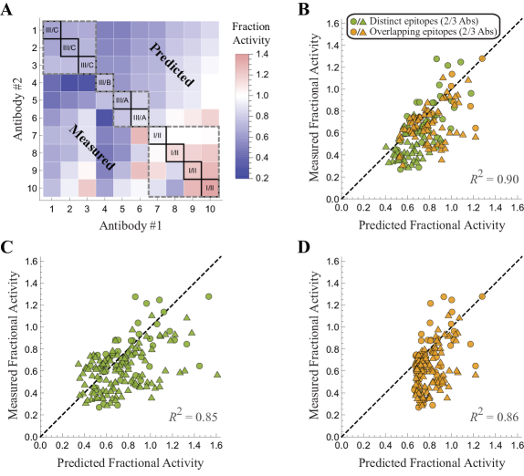
Figure 2: Predicting how antibody mixtures affect the epidermal growth factor receptor (EGFR). (A) The fractional activity of EGFR in the presence of monoclonal antibodies (diagonal) together with the measured (bottom-left) and predicted (top-right) activity of all 2-Ab combinations. The dashed gray boxes enclose antibody pairs that compete for the same epitope while all other pairs bind independently. (B) The predicted versus measured fractional activity for all 2-Ab and 3-Ab mixtures using the same epitope mapping as in Panel A inferred by SPR. Without the epitope map, the activity of the mixtures could alternately be predicted by assuming that all antibodies either (C) bind independently or (D) compete for the same epitope; in either case, the resulting predictions fall further from the diagonal line, indicating poorer predictive power.

On the other hand, antibodies #1 and #2 bind to the same epitope (III/C), and hence their predicted combined activity (0.67) lies between their individual activities (0.65 and 0.69) since both antibodies compete for the same site. The measured activity of the mixture (0.65) closely matches the prediction of the overlapping epitope model, but is very different than the prediction of 0.45 made by the distinct-binding model.

Fig 2B shows the measured EGFR activity in the presence of all 2-Ab and 3-Ab mixtures is highly correlated with the predicted activity ($R^{2}=0.90$) Notably, the predictions are made solely from the monoclonal antibody data and epitope measurements, and do not involve any fitting of the 2-Ab or 3-Ab measurements. The strong correlation between the predicted and measured activities suggests that EGFR antibody mixtures can be characterized with minimal synergistic effects in either their binding or effector functions. If we did not have the epitope mapping through SPR and assumed that all antibodies bound to distinct epitopes (Fig 2C, $R^{2}=0.85$) or competed for the same epitope (Fig 2D, $R^{2}=0.86$), the resulting predictions are slightly more scattered from the diagonal, demonstrating that properly acknowledging which pairs of antibodies vie for the same epitope boosts the predictive power of the model.

That said, the predictions incorporating the SPR mapping display a consistent bias towards having a slightly lower measured than predicted activity, suggesting that several pairs of antibody enhance one another’s binding affinity or potency. To quantify this, if we recharacterize the activity from the 2-Ab mixtures to a synergistic model where each $\alpha_{2,\text{eff}}$ is fit to exactly match the data, we find an average value of $\frac{\alpha_{2,\text{eff}}}{\alpha_{2}}=0.9$, showing that when pairs of antibodies are simultaneously bound they typically boost their collective inhibitory activity by $\sim$10%.

Differentiating distinct versus overlapping epitopes using antibody mixtures

In the previous section, we used SPR measurements to quantify which antibodies compete for overlapping epitopes, thereby permitting us to translate the molecular knowledge of antibody interactions into a macroscopic quantity of interest, namely, the activity of EGFR. In this section, we do the reverse and utilize activity measurements to categorize which subsets of antibodies bind to overlapping epitopes. This method can be applied to model antibody mixtures in other biological systems where SPR measurements are not readily available.

For the remainder of this section, we ignore the known epitope mappings discerned by Koefoed et al. and consider what mapping best characterizes the data. For example, given the individual activities of antibody #1 (0.65) and #2 (0.69), the predicted activity of their combination (at the concentration of $1\frac{\mu\text{g}}{\text{mL}}$ for each antibody dictated by the experiments) would be 0.45 if they bind to distinct epitopes and 0.67 if they bind to overlapping epitopes. Since the measured activity of this mixture was 0.65, it suggests the latter option. We note that such analysis will work best for potent antibodies (whose individual activity is far from 1), since only in this regime will the predictions of the distinct versus overlapping models be significantly different. Therefore, the activity measurements of each individual antibody would optimally be carried out at saturating concentrations (where Eq (1) is as far from 1 as possible).

Proceeding to the other antibodies, we characterize each pair according to whichever model prediction lies closer to the experimental measurement. To account for experimental error, we left an antibody pair uncategorized if the two model predictions were too close to one another (within $4\sigma=0.16$ where $\sigma$ is the SEM of the measurements) or if the experimental measurement was close (within $1\sigma$) to the average of the two model predictions (see S1 Text Section B).

Fig 3A shows how this analysis compares to the experimental measurement inferred by SPR. While the model predictions are much sparser (with the majority of antibody pairs uncategorized because the two model predictions were too close to one another), the classifications only disagreed with the SPR measurements in two cases (claiming that antibodies #7-8 overlap with antibody #10; notice that antibodies #7-8 have individual activities close to 1, making them difficult to characterize).

Using these classifications, we defined unique EGFR epitopes by grouping together any antibodies that bind to overlapping epitopes. In this way, we split the ten antibodies into four distinct groups (antibodies #1-3, #4-5, #6, and #7-10 indicated by the dashed gray rectangles in Fig 3A), enabling us to distinguish which antibodies bind independently or competitively and hence predict the activity of the 2-Ab and 3-Ab mixtures. Note that it is not the pairwise classification between two antibodies that determines whether we apply the distinct or competitive models, but rather these four groupings of antibody epitopes. For example, although antibodies #7 and #8 are uncategorized through their 2-Ab mixture, they fall within a single epitope group and hence are considered to bind competitively. Similarly, antibody #1 and #4 are modeled as binding independently because they belong to two distinct epitope groups. Antibody #6 is considered to be in its own epitope group since it did not overlap with any other antibody.

Surprisingly, the results shown in Fig 3B have a coefficient of determination $R^{2}=0.90$ that is on par with the results obtained using the SPR measurements (Fig 2B). This suggests that there is no loss in the predictive power of the model when an epitope mapping is inferred through activity measurements.

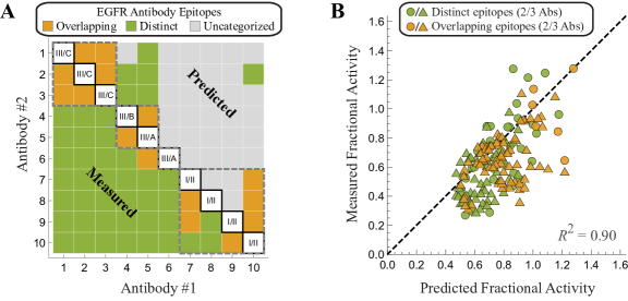
Figure 3: Classifying antibody epitopes as overlapping or distinct. (A) Comparing the experimentally measured activity to the overlapping or distinct epitope models enables us to characterize each antibody pair (provided the two models predict sufficiently different activities). (B) The resulting predictions for the 2-Ab and 3-Ab mixtures have the same predictive power ($R^{2}=0.90$) as a model that relies on epitope groupings given by SPR measurements (Fig 2B).

In summary, whether antibodies bind independently or competitively can be determined either: (1) directly through pairwise competition experiments or (2) by analyzing the activity of their 2-Ab mixtures in light of our two models. When this information is combined with the potency and dissociation constant of each antibody, the activity of an arbitrary mixture can be predicted. The Supplementary Information contains a Mathematica program that can analyze either form of the pairwise interactions to determine the epitope grouping. If the characteristics of the individual antibodies are also provided, the program can predict the activity of any antibody mixtures at any specified ratio of the constituents.

Multidomain antibodies boost breadth and potency via avidity

While the previous sections analyzed combinations of whole, unmodified antibodies, we now extend our framework to connect with the rising tide of engineering efforts that genetically fuse different antibody components to construct multi-domain antibodies [8]. Specifically, we focus our attention on recent work by Laursen et al. who isolated single-domain antibodies from llamas immunized with H2 or H7 influenza hemagglutinin (HA) [7]. The four single-domain antibodies isolated in this manner included one antibody that preferentially binds influenza A group 1 strains ($\text{Ab}_{\text{A1}}$), another that binds influenza A group 2 strains ($\text{Ab}_{\text{A2}}$), and two antibodies that bind to influenza B strains ($\text{Ab}_{\text{B}}^{(1)}$ and $\text{Ab}_{\text{B}}^{(2)}$). Fig 4A,B shows data from a representative influenza A group 1 strain (blue dot, only bound by the blue $\text{Ab}_{\text{A1}}$), influenza A group 2 strain (green dot, only bound by the green $\text{Ab}_{\text{A2}}$), and influenza B strain (gold dot, bound by both of the yellow $\text{Ab}_{\text{B}}^{(1)}$ and $\text{Ab}_{\text{B}}^{(2)}$ antibodies).

In the contexts of rapidly evolving pathogens such as influenza, two important characteristics of antibodies are their potency and breadth. Potency is measured by the inhibitory concentration $\text{IC}_{50}$ at which 50% of a virus is neutralized, where a smaller $\text{IC}_{50}$ represents a better antibody. Breadth is a measure of how many strains are susceptible to an antibody.

In an effort to improve the potency and breadth of their antibodies, Laursen et al. tethered together different domains using a flexible amino acid linker (right-most columns of Fig 4A,B) and tested them against a panel of influenza strains. To make contact with these multidomain constructs, consider a concentration $c$ of the tethered antibody $\text{Ab}_{\text{A1}}\text{\textendash}\text{Ab}_{\text{A2}}$. Relative to the unbound HA state, the $\text{Ab}_{\text{A1}}$ or $\text{Ab}_{\text{A2}}$ portions of the antibody will neutralize the virus with relative probability $\frac{c}{\text{IC}_{50,\text{A1}}}$ or $\frac{c}{\text{IC}_{50,\text{A2}}}$, respectively. Although neutralization is mediated by antibody binding, the two quantities may or may not be proportional [9, 10, 11], and hence we replace dissociation constants with $\text{IC}_{50}$s in our model (see S1 Text Section C).

Laursen et al. determined that their tethered constructs cannot intra-spike crosslink two binding sites on a single HA trimer, but they can inter-spike crosslink adjacent HA [7]. The linker connecting the two antibody domains facilitates such crosslinking, since when one domain is bound the other domain is confined to a smaller volume around its potential binding sites. This effect can be quantified by stating that the second domain has an effective concentration $c_{\text{eff}}$ (Fig 4C, purple), making the relative probability of the doubly bound state $\frac{c}{\text{IC}_{50,\text{A1}}}\frac{c_{\text{eff}}}{\text{IC}_{50,\text{A2}}}$. Therefore, the fraction of virus neutralized by two tethered antibody domains is given by

$$\text{Fraction Neutralized}=\frac{\frac{c}{\text{IC}_{50,\text{A1}}}+\frac{c}{\text{IC}_{50,\text{A2}}}+\frac{c}{\text{IC}_{50,\text{A1}}}\frac{c_{\text{eff}}}{\text{IC}_{50,\text{A2}}}}{1+\frac{c}{\text{IC}_{50,\text{A1}}}+\frac{c}{\text{IC}_{50,\text{A2}}}+\frac{c}{\text{IC}_{50,\text{A1}}}\frac{c_{\text{eff}}}{\text{IC}_{50,\text{A2}}}}.$$ (4)

Note that this equation assumes that influenza virus is fully neutralized at saturating concentrations of antibody ($\alpha=0$ in Eq (1), with Fraction Neutralized analogous to $1-\text{Fractional Activity}$).

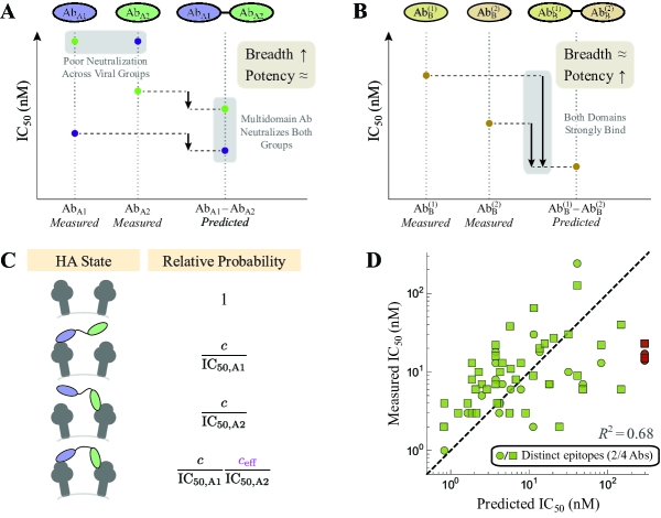
Figure 4: Tethering influenza antibodies increases breadth and potency. (A) The influenza A antibodies $\text{Ab}_{\text{A1}}$ and $\text{Ab}_{\text{A2}}$ were tethered together to form $\text{Ab}_{\text{A1}}\text{\textendash}\text{Ab}_{\text{A2}}$ while (B) two influenza B antibodies formed $\text{Ab}_{\text{B}}^{(1)}\text{\textendash}\text{Ab}_{\text{B}}^{(2)}$. Representative data shown for an influenza A group 1 (blue), influenza A group 2 (green), and influenza B (gold) strains. Strong potency is marked by a small $\text{IC}_{50}$ while large breadth implies that multiple strains are controlled by an antibody. (C) Representative states of HA and their corresponding Boltzmann weights for multidomain antibodies, where crosslinking between adjacent spikes boosts neutralization via avidity ($c_{\text{eff}}=1400\,\text{nM}$ in Eq (5)). (D) Theoretical predictions of the potency of all multidomain antibodies versus their measured values. The red points denote two outlier influenza strains discussed in the text that are not neutralized by $\text{Ab}_{\text{A1}}$ or $\text{Ab}_{\text{A2}}$ individually but are highly neutralized by their combination.

The $\text{IC}_{50}$ of the tethered construct is defined as the concentration $c$ at which half of the virus is neutralized, which can be solved to yield

$$\text{IC}_{\text{50,A1\text{\textendash}A2}}=\frac{\text{IC}_{\text{50,A1}}\,\text{IC}_{\text{50,A2}}}{c_{\text{eff}}+\text{IC}_{\text{50,A1}}+\text{IC}_{\text{50,A2}}},$$ (5)

with an analogous expression holding for the $\text{Ab}_{\text{B}}^{(1)}\text{\textendash}\text{Ab}_{\text{B}}^{(2)}$ construct. Using the measured $\text{IC}_{50}$s of $\text{Ab}_{\text{A1}}\text{\textendash}\text{Ab}_{\text{A2}}$ and $\text{Ab}_{\text{B}}^{(1)}\text{\textendash}\text{Ab}_{\text{B}}^{(2)}$ against the various influenza strains, we can infer the value of the single parameter $c_{\text{eff}}=1400\,\text{nM}$ (see S1 Text Section C). This result is both physically meaningful and biologically actionable, as it enables us to predict the $\text{IC}_{50}$ of the tethered multidomain antibodies against the entire panel of influenza strains. Fig 5A,B compares the resulting predictions to the experimental measurements, where plot markers linked by horizontal line segments indicate a close match between the predicted and measured values.

The two tethered antibodies display unique trends that arise from their compositions. Since the two domains in $\text{Ab}_{\text{A1}}\text{\textendash}\text{Ab}_{\text{A2}}$ bind nearly complementary strains, the tethered construct will increase breadth (since this multidomain antibodies can now bind to both group 1 and group 2 strains) but will only marginally improve potency. Mathematically, if $\text{Ab}_{\text{A1}}$ binds tightly to an influenza A group 1 strain while $\text{Ab}_{\text{A2}}$ binds weakly to this same strain ($\text{IC}_{\text{50,A2}}\to\infty$), their tethered construct has an $\text{IC}_{\text{50,A1\text{\textendash}A2}}\approx\text{IC}_{\text{50,A1}}$. Said another way, $\text{Ab}_{\text{A1}}\text{\textendash}\text{Ab}_{\text{A2}}$ should be approximately as potent as a mixture of the individual antibodies $\text{Ab}_{\text{A1}}$ and $\text{Ab}_{\text{A2}}$. Note that since the experiments could not accurately measure weak binding ($>1000\,\text{nM}$), the predicted $\text{IC}_{50}$ for the multidomain antibodies represents a lower bound.

On the other hand, tethering the two influenza B antibodies yields a marked improvement in potency over either individual antibody, since both domains can bind to any influenza B strain and boost neutralization via avidity. The process of engineering a multivalent interaction is reminiscent of engineered bispecific IgG [8], and adding additional domains could yield further enhancement in potency, provided that all domains can simultaneously bind.

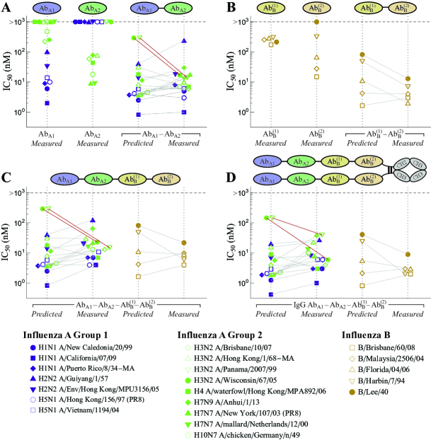
Figure 5: Neutralization of multidomain antibodies. (A,B) The potency of the 2-Ab constructs and their constitutive antibodies against a panel of influenza strains. $\text{Ab}_{\text{A1}}$ primarily binds influenza A group 1 (blue), $\text{Ab}_{\text{A2}}$ to influenza A group 2 (green), and the two $\text{Ab}_{\text{B}}$ antibodies to influenza B strains (gold). (C) All four antibodies were tethered to form the linear chain $\text{Ab}_{\text{A1}}\text{\textendash}\text{Ab}_{\text{A2}}\text{\textendash}\text{Ab}_{\text{B}}^{(1)}\text{\textendash}\text{Ab}_{\text{B}}^{(2)}$ and (D) two copies of this chain were placed on an IgG backbone. The model suggests that the two arms of the IgG are not capable of simultaneously binding a virion. Red lines indicate two outlier influenza strains discussed in the text that are not neutralized by $\text{Ab}_{\text{A1}}$ or $\text{Ab}_{\text{A2}}$ individually but are highly neutralized by their combination. Data was digitized from Figs 1 and 3 of Ref [7].

While the model is able to characterize the majority of tethered antibodies, it also highlights some of the outliers in the data. For example, the H3N2 strains A/Panama/2007/99 and A/Wisconsin/67/05 were poorly neutralized by either $\text{Ab}_{\text{A1}}$ or $\text{Ab}_{\text{A2}}$ ($\text{IC}_{50}\geq 1000\,\text{nM}$), but the tethered construct exhibited an $\text{IC}_{50}=14\,\text{nM}$ and $\text{IC}_{50}=17\,\text{nM}$, respectively, far more potent than the $300\,\text{nM}$ lower limit predicted for both viruses (red circles in Fig 4D and red lines in Fig 5A). Interestingly, Laursen et al. found that mixing the individual, untethered antibodies $\text{Ab}_{\text{A1}}$ and $\text{Ab}_{\text{A2}}$ also resulted in shockingly poor neutralization ($\text{IC}_{50}\geq 1000\,\text{nM}$), suggesting that the tether is responsible for the increase in potency [7]. From the vantage of our quantitative model, this outlier cries out for further investigation.

To further boost neutralization, Laursen et al. created two additional constructs that combined all four antibody domains, the first being the linear chain ($\text{Ab}_{\text{A1}}\text{\textendash}\text{Ab}_{\text{A2}}\text{\textendash}\text{Ab}_{\text{B}}^{(1)}\text{\textendash}\text{Ab}_{\text{B}}^{(2)}$). Since the influenza A antibodies do not bind the influenza B strains (and vise versa), this construct should have the same $\text{IC}_{50}$ as $\text{Ab}_{\text{A1}}\text{\textendash}\text{Ab}_{\text{A2}}$ for the influenza A strains and as $\text{Ab}_{\text{B}}^{(1)}\text{\textendash}\text{Ab}_{\text{B}}^{(2)}$ for the influenza B strains, as was found experimentally (compare the Predicted columns in Fig 5A-C). For example, the two H3N2 strains (A/Panama/2007/99 and A/Wisconsin/67/05) were again found to have measured $\text{IC}_{50}$s ($15\,\text{nM}$ and $23\,\text{nM}$) far smaller than their predicted lower bound of $300\,\text{nM}$ (red squares in Fig 4D, red lines in Fig 5C).

A second construct containing all four antibody domains attached two copies of $\text{Ab}_{\text{A1}}\text{\textendash}\text{Ab}_{\text{A2}}\text{\textendash}\text{Ab}_{\text{B}}^{(1)}\text{\textendash}\text{Ab}_{\text{B}}^{(2)}$ through an IgG backbone (Fig 5D). Since the identical domains in both arms of this construct should be able to simultaneously bind, the new antibody should markedly boost potency through avidity. Surprisingly, the neutralization of this final construct was well characterized as half the $\text{IC}_{50}$ of an individual $\text{Ab}_{\text{A1}}\text{\textendash}\text{Ab}_{\text{A2}}\text{\textendash}\text{Ab}_{\text{B}}^{(1)}\text{\textendash}\text{Ab}_{\text{B}}^{(2)}$, suggesting that there was no noticeable avidity and that the increase in neutralization only arose from having twice as many antibody domains. As above, this intriguing result presents an opportunity to both quantitatively check experimental results and to advocate for future studies in potentially highly promising directions. In this particular instance, it suggests that the IgG backbone used did not permit simultaneous binding of both arms. If a different multivalent scaffold (perhaps with greater flexibility or with longer linkers) enabled bivalent binding of both arms, it could potentially increase the neutralization of this construct by 100-fold as seen in the influenza B constructs.

Discussion

In this work, we developed a statistical mechanical model that predicts the collective efficacy of an antibody mixture whose constituents are assumed to bind to a single site on a receptor. Each antibody is first individually characterized by its ability to bind the receptor (through its dissociation constant $K_{D}$) and inhibit activity (via its potency $\alpha$) as per Eq (1). Importantly, this implies that the activity of each monoclonal antibody must be measured at a minimum of two concentrations in order to infer both parameters, and additional measurements would further refine these parameter values and the corresponding model predictions.

After each antibody is individually characterized, the activity of a combination of antibodies will depend upon whether they bind independently to distinct epitopes or compete for overlapping epitopes. Theoretical models often assume for simplicity that all antibodies bind independently, and in the contexts where this constraint can be experimentally imposed such models can accurately predict the effectiveness of antibody mixtures [12]. Yet when the antibody epitopes are unknown or when a large number of antibodies are combined, it is likely that some subset of antibodies will compete with each other while others will bind independently, which will give rise to a markedly different response. Our model generalized these previous results to account for antibody mixtures where arbitrary subsets can bind independently or competitively (Eqs (2) and (3), S1 Text Section A).

We showed that in the context of the EGFR receptor, where every pairwise interaction was measured using surface plasmon resonance, our model is better able to predict the efficacy of all 2-Ab and 3-Ab mixtures than a model that assumes all antibodies bind independently or competitively (Fig 2). This suggest that mixtures of antibodies do not exhibit large synergistic effects. More generally, similar models in the contexts of anti-cancer drug cocktails and anti-HIV antibody mixtures also found that the majority of cases that were described as synergistic could instead be characterized by an independent binding model [13, 12]. This raises the possibility that synergy is more the exception then the norm, and hence that simple models can computationally explore the full design space of antibody combinations.

While it is often straightforward to measure the efficacy of $n$ individual antibodies, it is more challenging to quantify all $\frac{n(n+1)}{2}$ pairwise interactions and determine which antibodies bind independently and which compete for an overlapping epitope. We demonstrated that after each antibody is individually characterized, our model can be applied in reverse by using the activity of 2-Ab mixtures to classify whether antibodies compete or bind independently (Fig 3). Surprisingly, while the resulting categorizations were much sparser than the direct SPR measurements, the classifications produced by this method predicted the efficacy of antibody combinations with an $R^{2}=0.90$, comparable to the predictions made using the complete SPR results (Fig 2B). This suggests that key features of how antibodies interact on a molecular level can be indirectly inferred from simple activity measurements of antibody combinations.

Modern bioengineering has opened up a new avenue of mixing antibodies by genetically fusing different components to construct multi-domain antibodies [8]. Such antibodies can harness multivalent interactions to greatly increase binding avidity by over 100x (e.g. comparing the $\text{IC}_{50}$s of the A/Wisconsin/67/05 and B/Harbin/7/94 strains of the 4-fused domains on an IgG backbone in Fig 5D to the corresponding $\text{IC}_{50}$s for the individual antibody domains in Panels A and B). For such constructs, the composition of the linker can heavily influence the ability to multivalently bind and neutralize a virus [14, 11], although Laursen et al. surprisingly found little variation when they modified the length of their amino acid linker (see Table S11 in Ref [7]). Another curious feature of their system was that placing their linear 4-domain antibody (Fig 5C) on an IgG backbone (Fig 5D) only resulted in a 2x decrease in $\text{IC}_{50}$, suggesting that the two “arms” of the IgG could not simultaneously bind. We would expect that a different backbone that allows both arms to simultaneously bind would markedly increase the neutralization potency of this construct. In this way, quantitatively modeling these multidomain antibodies can guide experimental efforts to design more potent constructs.

To close, we mention that two possible avenues of future work. First, although our model classifies antibody epitopes as either distinct or overlapping, SPR measurements indicate that there is a continuum of possible interactions. It would be fascinating to translate this more nuanced level of interaction into more precise dissociation constants when two antibodies are bound. Second, while our model focused on mixtures of antibodies, it can be applied equally well to small molecule drugs where the number of distinct combinations may be prohibitively large to measure experimentally but straightforward to explore computationally.

Methods

The coefficient of determination used to quantify how well the theoretical predictions matched the experimental measurements (Fig 2B-D, Fig 3B, Fig 4D) was calculated using

$$R^{2}=1-\frac{\sum_{j=1}^{n}\left(y_{\text{measured}}^{(j)}-y_{\text{predicted}}^{(j)}\right)^{2}}{\sum_{j=1}^{n}\left(y_{\text{data}}^{(j)}\right)^{2}}$$ (6)

where $y_{\text{measured}}$ and $y_{\text{predicted}}$ represent a vector of the measured and predicted activities for the $n$ mixtures analyzed. In Fig 4D, we computed the $R^{2}$ of $\log_{10}(\text{activity})$ to prevent the largest activities from dominating the result (since the $\text{IC}_{50}$ values span multiple decades).

Data from the EGFR antibody mixtures was obtained by digitizing Ref [6] Fig S1 using WebPlotDigitizer [15]. Data for the influenza multidomain antibodies was obtained from the authors of Ref [7].

The EGFR antibody epitopes experimentally characterized through SPR (Fig 3A, bottom-left) were categorized as overlapping if the average of the two antibody measurements (with preincubation by either antibody) were $>50$ and as distinct if the average was $<50$.

The original nomenclature for the antibodies used in Koefoed et al. and Laursen et al. are given in S1 Text Table S1.

Appendix A Characterizing Antibodies Targeting the Receptor Tyrosine Kinase EGFR

A.1 Monoclonal Antibody Binding to a Receptor

In this section, we explain the states and weights notation used to develop the equilibrium statistical mechanical models used in this work. As a focus, we consider the case of an antibody binding to a single site on a receptor as shown in Fig S1A. We assume that the concentration of the antibody far exceeds that of the receptor, so that one binding event will not noticeably affect the concentration $c$ of free antibody.

The receptor can exist in two states where it is either unbound or bound to the antibody, where the relative probability of the bound state compared to the unbound state equals $\frac{c}{K_{D}}$, where $K_{D}$ is the dissociation constant of the receptor-antibody binding [16]. The (normalized) probability of each state is given by its relative weight divided by the sum of the relative weights of all states. For example, the probability that the receptor is bound to the antibody is shown to be the standard $\frac{\frac{c}{K_{D}}}{1+\frac{c}{K_{D}}}$ sigmoidal response. As expected, the receptor will always be unbound in the absence of antibody ($c=0$), while the receptor will always be bound at saturating concentrations of antibody ($c\to\infty$).

Each receptor state also has a relative activity (i.e. the activity of the receptor when it is in this state). In the context of EGFR, where the fractional activity is measured relative to the receptor in the absence of antibody, the relative activity of the unbound state is by definition equal to 1. As in the main text, we define the activity of the bound receptor to be $\alpha$, where $\alpha=0$ implies that the receptor is completely inactive when the antibody is bound and $\alpha=1$ represents the opposite limit where antibody binding does not inhibit the receptor’s activity. A value of $0<\alpha<1$ represents an antibody that partially inhibits activity upon binding.

The activity of the receptor in each state is given by the product of its relative activity and the normalized probability of that state. Lastly, the average activity of the receptor is given by the sum of its activity in each state,

$$\text{Activity}=\frac{1+\alpha\frac{c}{K_{D}}}{1+\frac{c}{K_{D}}}.$$ (S1)

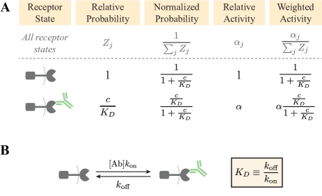
Figure S1: A statistical mechanical model of an antibody binding to a receptor. (A) The relative probability and relative activity of each receptor state enable us to derive the average activity of the receptor. (B) This method gives the same result of the dynamics model shown by the multiple rates, provided that the system is in steady state.

As a quick aside, we note out that all the models considered in this work analyze binding reactions that quickly reach steady, and hence the equilibrium model derived above will should accurately describe such systems. Eq (S1) can also be derived by considering the dynamics of the system shown in the rates diagram Fig S1B. The unbound receptor (R) will switch to the bound state (R–Ab) at the rate $ck_{\text{on}}$ (recall that $c$ is the concentration of antibody) and subsequently unbind at a rate $k_{\text{off}}$. Hence, the system is governed by the two differential equations

$$\frac{d[\text{R}]}{dt} =k_{\text{off}}[\text{R}\text{\textendash}\text{Ab}]-ck_{\text{on}}[\text{R}]$$ (S2)

$$\frac{d[\text{R}\text{\textendash}\text{Ab}]}{dt} =ck_{\text{on}}[\text{R}]-k_{\text{off}}[\text{R}\text{\textendash}\text{Ab}].$$ (S3)

Since the total amount of receptor $[\text{R}_{\text{tot}}]=[\text{R}]+[\text{R}\text{\textendash}\text{Ab}]$ is fixed, these two equations are equivalent, and either one can be solved to yield the dynamics of the system, namely,

$$[R]=c_{1}e^{-\left(k_{\text{off}}+ck_{\text{on}}\right)t}+[\text{R}_{\text{tot}}]\frac{k_{\text{off}}}{k_{\text{off}}+ck_{\text{on}}}.$$ (S4)

$c_{1}$ is fixed by the initial concentration of free receptor $[R]$ at $t=0$, but regardless of its value, we see that the exponential term will shrink to zero at a time scale of $\frac{1}{k_{\text{off}}+ck_{\text{on}}}$, after which the system will be in steady state with $[R]=[\text{R}_{\text{tot}}]\frac{k_{\text{off}}}{k_{\text{off}}+ck_{\text{on}}}$. Defining the dissociation constant $K_{D}\equiv\frac{k_{\text{off}}}{k_{\text{on}}}$, the probability that any receptor will be unbound in steady state is given by

$$\frac{[R]}{[\text{R}_{\text{tot}}]}=\frac{1}{1+\frac{c}{K_{D}}}$$ (S5)

as found in Fig S1A.

To close, we note that antibodies typically have a $K_{D}=10^{-12}\text{\textendash}10^{-8}\,\text{M}$, and assuming a diffusion-limited on rate $k_{\text{on}}=10^{8}\text{\textendash}10^{-9}\,\frac{1}{\text{M}\cdot\text{s}}$, this implies that $k_{\text{off}}=10^{-3}\text{\textendash}10^{1}\,\frac{1}{\text{s}}$. Therefore, an upper bound (in the limit of little antibody) for the time scale it takes for such a system to reach steady state is $10^{-1}\text{\textendash}10^{3}\,\text{s}$, which is the time before experimental measurements should be conducted. Since antibodies are typically preincubated for even longer periods during experiments, an equilibrium model should be valid in all of the case studies we consider in this work.

A.2 The Fractional Activity of 3-Ab Mixtures

As described in the main text, the fractional activity of 2-Ab mixtures is given by Eq 2 if the two antibodies bind to distinct epitopes and Eq 3 if they bind to overlapping epitopes. These equations are straightforward to extend to mixtures with multiple antibodies by drawing all of the statistical weights and Boltzmann weights for the mixture (analogous to Fig 1) and then computing the fractional activity as per Section A.1.

For example, a mixture of three antibodies all binding to distinct epitopes would give rise to

$$\text{Fractional Activity}_{\text{(1,2,3 distinct epitopes)}}=\left(\frac{1+\alpha_{1}\frac{c_{1}}{K_{D}^{(1)}}}{1+\frac{c_{1}}{K_{D}^{(1)}}}\right)\left(\frac{1+\alpha_{2}\frac{c_{2}}{K_{D}^{(2)}}}{1+\frac{c_{2}}{K_{D}^{(2)}}}\right)\left(\frac{1+\alpha_{3}\frac{c_{3}}{K_{D}^{(3)}}}{1+\frac{c_{3}}{K_{D}^{(3)}}}\right).$$ (S6)

If antibodies 1 and 2 bind to an overlapping epitope but antibody 3 binds to a distinct epitope, then

$$\text{Fractional Activity}_{\text{(1,2 overlapping epitopes; 3 distinct epitope)}}=\left(\frac{1+\alpha_{1}\frac{c_{1}}{K_{D}^{(1)}}+\alpha_{2}\frac{c_{2}}{K_{D}^{(2)}}}{1+\frac{c_{1}}{K_{D}^{(1)}}+\frac{c_{2}}{K_{D}^{(2)}}}\right)\left(\frac{1+\alpha_{3}\frac{c_{3}}{K_{D}^{(3)}}}{1+\frac{c_{3}}{K_{D}^{(3)}}}\right).$$ (S7)

If all three antibodies binds to overlapping epitopes, the fractional activity becomes

$$\text{Fractional Activity}_{\text{(1,2 overlapping epitopes; 3 distinct epitope)}}=\frac{1+\alpha_{1}\frac{c_{1}}{K_{D}^{(1)}}+\alpha_{2}\frac{c_{2}}{K_{D}^{(2)}}+\alpha_{3}\frac{c_{3}}{K_{D}^{(3)}}}{1+\frac{c_{1}}{K_{D}^{(1)}}+\frac{c_{2}}{K_{D}^{(2)}}+\frac{c_{3}}{K_{D}^{(3)}}}.$$ (S8)

A.3 Characterizing Ten EGFR Monoclonal Antibodies from Koefoed 2011

Koefoed et al. investigated how a panel of ten monoclonal antibodies inhibit EGFR by measuring the protein’s activity at multiple antibody concentrations in the human cell line HN5 [6]. By fitting these titration curves to Eq 1, we can infer the dissociation constant $K_{D}$ between each antibody and EGFR as well as the potency $\alpha$ of each antibody in the HN5 cell line (Fig S2A,B). For each curve, the $K_{D}$ corresponds to the midpoint of the curve (halfway between its minimum and maximum activity values) while $\alpha$ represents the activity at saturating antibody concentration.

Koefoed et al. found that the majority (7/10) of these antibodies reduced EGFR activity below 20% at saturating concentrations, and since mixtures of antibodies would likely further decrease activity their potency would be difficult to accurately measure. To that end, Koefoed et al. switched to the A431NS cell line that is partially resistant to EGFR antibodiess where they remeasured EGFR activity for all ten monoclonal antibodies as well as mixtures of two or three Abs (with 1:1 and 1:1:1 ratios, respectively). Each measurement was performed at a mixture concentration of $2\frac{\mu\text{g}}{\text{mL}}$, implying that each antibody was half as dilute in the 2-Ab mixtures and one-third as dilute in the 3-Ab mixtures relative to the monoclonal antibody measurement.

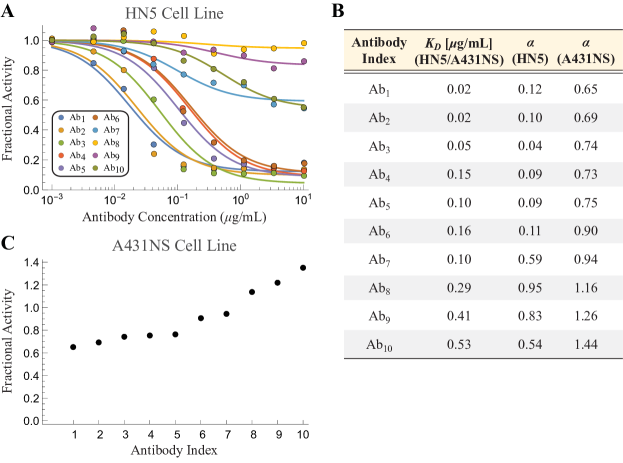
Figure S2: Inferring the model parameters for the 10 monoclonal antibodies in Koefoed 2011. (A) Activity of EGFR in the presence of ten antibodies in the HN5 cell line. (B) The inferred dissociation constant ($K_{D}$) and fractional activity in the presence of saturating antibody ($\alpha$) in each cell line. (C) Fractional EGFR activity in the presence of $2\frac{\mu\text{g}}{\text{mL}}$ of each antibody in the A431NS cell line. Data reproduced from Ref [6] Figure 2B,C.

We assume that the antibody-EGFR binding interaction is identical in the A431NS cell line, and hence that these same $K_{D}$ parameters characterizes these antibodies in that cell line. Hence, by using the additional measurement of each antibody’s potency at $2\frac{\mu\text{g}}{\text{mL}}$ in the A431NS cell line (Fig S2C), we can infer the potency $\alpha$ of each antibody in the A431NS cell line (Fig S2B). These parameters are sufficient to predict how any mixture (at any concentration and ratio) will behave in the HN5 and A431NS cell lines. Note that all data presented in the main text correspond to the A431NS cell line.

A.4 Comparing the HN5 and A431NS Cell Lines from Koefoed 2011

Koefoed et al. measured the potency of 176 mixtures in the A431NS cell line but only 55 mixtures in the HN5 cell line. Fig S3 extends our analysis to both the A431NS and HN5 cell lines. While the majority of mixtures have very little predicted and measured activity ($\lesssim 0.2$), approximately 13 outliers fall outside this range and appear to be poorly predicted.

While the coefficient of determination $R^{2}=0.61$ is significantly lower for this cell line, we note that: (1) there are far fewer data points in this cell line and (2) that our $R^{2}$ definition places more importance on points with larger predicted or measured fractional activity, and hence these few outliers have a disproportionate effect. That said, it remains unknown whether with more data our model would be as successful in the HN5 cell line. Another open question is why some antibody mixtures had inhibitory effects in one cell line but exacerbating effects in the other (e.g. the mixture of $\text{Ab}_{3}+\text{Ab}_{10}$ resulted in 1.22 fractional activity of EGFR in the A431NS cell line but 0.19 fractional activity in the HN5 cell line).

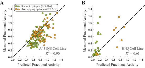
Figure S3: Predicting the potency of antibody mixtures on EGFR in different cell lines. Our model predictions versus experimental measurements for EGFR activity in the (A) A431NS and (B) HN5 cell lines.

A.5 Separating the 2-Ab and 3-Ab Predictions for EGFR Antibody Mixtures

Fig S4 separates the 2-Ab and 3-Ab mixture predictions from the three models in Fig 2. More specifically, Panels A and B of Fig S4 show the predictions for combinations of two and three antibodies using the epitope mappings produced by SPR (see captions on the diagonal of Fig 2A; there are four EGFR epitopes bound by antibodies #1-3, #4, #5-6, and #7-10, respectively).

Without this SPR data, we could have alternately assumed that antibodies all bind independently (Fig S4C,D) or that all antibodies vie for the same epitope (Fig S4E,F). Either of these models generate slightly worse predictions, as exhibited by their lower coefficients of determination $R^{2}$.

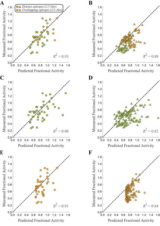
Figure S4: Separate predictions for 2-Ab and 3-Ab mixtures. (A,B) Predictions using the epitope mappings produced using SPR. (C,D) Predictions assuming that all antibodies bind independently. (E,F) Predictions assuming that all antibodies bind competitively.

A.6 Original Antibody Nomenclature

Table S1 shows the antibodies considered in this work were named in the original works of Refs. [6] and [7]. In our work, we indexed the EGFR antibodies by their potency in the A431NS cell line and labeled the influenza antibodies by the viral group that they most effectively neutralized.

Koefoed 2011 Antibody Nomenclature			Laursen 2018 Antibody Nomenclature
…..This Work…..	Original Work		…..This Work…..	Original Work
$\text{Ab}_{1}$	1565		$\text{Ab}_{\text{A1}}$	SD38
$\text{Ab}_{2}$	1320		$\text{Ab}_{\text{A2}}$	SD36
$\text{Ab}_{3}$	1024		$\text{Ab}_{\text{B}}^{(1)}$	SD83
$\text{Ab}_{4}$	992		$\text{Ab}_{\text{B}}^{(2)}$	SD84
$\text{Ab}_{5}$	1277
$\text{Ab}_{6}$	1030
$\text{Ab}_{7}$	1284
$\text{Ab}_{8}$	1347
$\text{Ab}_{9}$	1260
$\text{Ab}_{10}$	1261

Table S1: Matching the antibody nomenclature used in this work with the names in the original manuscript.

Appendix B Characterizing Distinct versus Overlapping EGFR Epitopes

In this section, we describe in more detail how we can use activity data from the 2-Ab mixtures to classify which subsets of antibodies bind to the same epitopes. A basic classification scheme would categorize two antibodies as binding to distinct epitopes if Eq 2 predicted their mixture’s activity better than Eq 3; otherwise, the two antibodies would be categorized as binding to overlapping epitopes.

However, this simple classification scheme does not account for the uncertainty that arises from experimental noise. As an extreme case, if the activities of a mixtures are measured at extremely small concentrations, then the fractional activity will be $\approx 1$ for all mixtures (as will be the predictions from both the distinct and overlapping models), and this classification scheme would only be fitting the noise. Hence, it is best to measure the activity of each mixture at saturating antibody concentrations where the signal-to-noise of the system will be greatest.

We determined from Koefoed et al. (Figure S1) that the standard error of the mean (SEM) of their activity measurements was $\sigma=0.04$, and we proceed to incorporate this uncertainty into our categorization scheme using a simple threshold model. More specifically, we add two components to the classification scheme: (1) As shown in Fig S5A, activity measurements that fall within $\sigma$ of the midpoint of the two model predictions are left unclassified, since experimental noise could easily lead to such points being incorrectly classified. (2) If the two model predictions lie sufficiently close (within $4\sigma$) to one another, then the uncertainty (from both the measurement and the model predictions) make it difficult to distinguish between the two models with certainty.

As mentioned above, for potent antibodies that are measured at saturating concentrations, the difference between the independent and overlapping binding models will be large, making it easier to definitively classify antibody epitopes. Koefoed et al. measured their 2-Ab combinations at a total concentration of $2\,\frac{\mu\text{g}}{\text{mL}}$ (and hence $1\,\frac{\mu\text{g}}{\text{mL}}$ for each antibody), and Fig S2A suggest that while this is close to saturating concentration for the majority of antibodies, increasing the concentration by 10x may have allowed more pairs of antibodies to be definitively categorized.

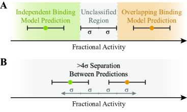
Figure S5: Accounting for uncertainty in the classification scheme. (A) 2-Ab combinations whose activity falls within $\sigma$ of the midpoint between the two model predictions will be labeled as “unclassified,” since the difference in distance from the measurement to either prediction is less than the experimental error. (B) In addition, when the two model predictions are less than $4\sigma$ different, any measurement is labeled as “unclassified” because measurement error could result in overlap with both model predictions.

Appendix C Characterizing Multidomain Antibodies

C.1 Relating Influenza Neutralization to Binding

In this section, we discuss how the microscopic dissociation constants of two tethered antibodies (shown in Fig 4C) relate to influenza viral neutralization. We begin by considering a single antibody with an effective dissociation constant $K_{D}^{(1)}$ that quantifies its avidity to the virus [17]. The probability that this antibody at concentration $c$ will be bound to a virion is given by

$$p_{\text{bound}}=\frac{\frac{c}{K_{D}^{(1)}}}{1+\frac{c}{K_{D}^{(1)}}}.$$ (S9)

For influenza virus with $N\approx 400$ hemagglutinin (HA) trimers, the number of bound trimers is given by $N_{\text{bound}}=Np_{\text{bound}}$.

The relationship between viral binding and neutralization remain unclear [18]. It has been suggested that $\sim 50$ HA trimers are required to infect a cell [17]. However, an IgG bound to one trimer may sterically preclude neighboring HA from binding. It has been proposed that neutralization is a sigmoidal function of neutralization (see Figure S1 of Ref [10]),

$$\text{Fraction Neutralized}=\frac{N^{h}+N_{50}^{h}}{N^{h}}\frac{\left(Np_{\text{bound}}\right)^{h}}{\left(Np_{\text{bound}}\right)^{h}+N_{50}^{h}},$$ (S10)

where $N_{50}$ is the number of bound trimers required to reduce infectivity to 50%, $h$ is a Hill coefficient, and the prefactor assures that the fraction neutralized ranges from 0 (in the absence of antibody) to 1 (in the presence of saturating antibody).

In the absence of data for our influenza strain of interest, we will assume $h=1$ in the following analysis. This enables us to rewrite Eq (S10) as

$$\text{Fraction Neutralized}=\frac{\frac{c}{\text{IC}_{50}^{(1)}}}{1+\frac{c}{\text{IC}_{50}^{(1)}}},$$ (S11)

where we have defined the inhibitory concentration of antibody at which 50% of the virus is neutralized

$$\text{IC}_{50}^{(1)}=\frac{N_{50}}{N+N_{50}}K_{D}^{(1)}.$$ (S12)

For example, if the virus is 50% neutralized when $N_{50}=100$ trimers are bound, the midpoint of a viral neutralization curve would occur at roughly $\nicefrac{{1}}{{5}}$ the antibody concentration required to bind 50% of the trimers, as has been observed for some influenza antibodies (see Figure 2 of Ref [9]).

We now consider the tethered two-domain antibody shown in Fig 4C. Denote the antibody concentration as $c$, the effective dissociation constants of its two domains as $K_{D}^{(1)}$ and $K_{D}^{(2)}$, and the effective concentration when both domains simultaneously bind as $\tilde{c}_{\text{eff}}$ (which we will shortly relate to the $c_{\text{eff}}$ in the antibody neutralization given in Eq 4). The probability that this antibody is bound to a virion is given by

$$p_{\text{bound}}=\frac{\frac{c}{K_{D}^{(1)}}+\frac{c}{K_{D}^{(2)}}+\frac{c}{K_{D}^{(1)}}\frac{\tilde{c}_{\text{eff}}}{K_{D}^{(1)}}}{1+\frac{c}{K_{D}^{(1)}}}.$$ (S13)

As above, we assume that neutralization is related to the binding probability through Eq (S10) with Hill coefficient $h=1$, which upon substituting Eq (S13) yields

$$\text{Fraction Neutralized}=\frac{\frac{c}{\text{IC}_{50,\text{A1}}}+\frac{c}{\text{IC}_{50,\text{A2}}}+\frac{c}{\text{IC}_{50,\text{A1}}}\frac{c_{\text{eff}}}{\text{IC}_{50,\text{A2}}}}{1+\frac{c}{\text{IC}_{50,\text{A1}}}+\frac{c}{\text{IC}_{50,\text{A2}}}+\frac{c}{\text{IC}_{50,\text{A1}}}\frac{c_{\text{eff}}}{\text{IC}_{50,\text{A2}}}}$$ (S14)

where we have defined the $\text{IC}_{50}$s of both antibodies using Eq (S12) as well as the rescaled effective concentration

$$c_{\text{eff}}=\frac{N_{50}}{N+N_{50}}\tilde{c}_{\text{eff}}.$$ (S15)

Therefore, in the case where $h=1$ the functional form of neutralization (Eq (S14)) is identical to the probability that an HA trimer is bound (Eq (S13)), with the dissociation constants and the effective concentration rescaled by $\frac{N_{50}}{N+N_{50}}$.

To put these results into perspective, we note that many viruses are covered in spikes (analogous to influenza HA) that enable them to bind and fuse to their target cells [18], and hence the sigmoidal dependence between viral binding and neutralization is likely widely applicable. However, HIV is a clear exception, since each virion has an average of 14 envelope spikes [19]. In that context, neutralization is roughly proportional to the number of bound spikes so that $\text{IC}_{50}\approx K_{D}$ [20].

C.2 Assuming Different Antibody Constructs have Distinct Effective Concentrations

In the main text, we quantified the boost in avidity from tethering two antibodies using the effective concentration $c_{\text{eff}}=1400\,\text{nM}$ by using least-squares regression to minimize the (log) predicted $\text{IC}_{50}$ for each tethered construct binding to all strains. This effective concentration depends on the distance between binding sites on a virion, and hence the tethered $\text{Ab}_{\text{A1}}\text{\textendash}\text{Ab}_{\text{A2}}$ construct may have a different $c_{\text{eff}}$ when binding to influenza A group 1 and group 2 strains, and $\text{Ab}_{\text{B}}^{(1)}\text{\textendash}\text{Ab}_{\text{B}}^{(2)}$ may have yet another effective concentration when binding to the influenza B strains.

Fig S6 shows the best-fit $c_{\text{eff}}$ for each of these cases. While this plot suggests that there are differences between each tethered antibody and influenza strain, we note that there is very limited data to infer such values (e.g., there are 7, 7, and 5 data points in the influenza A1, A2, and B groups, respectively; note that we ignore the H3N2 outlier strains A/Panama/2007/99 and A/Wisconsin/67/05 discussed in the main text). That said, incorporating this fine-grained level of modeling could further boost the accuracy of modeling efforts and is worth pursuing as more data is gathered.

Finally, we mention that Laursen et al. measured the efficacy of $\text{Ab}_{\text{A1}}\text{\textendash}\text{Ab}_{\text{A2}}$ with different linkers of length 18 amino acids ($\sim 63\text{\AA}$), 38 amino acids ($\sim 133\text{\AA}$), and 60 amino acids ($\sim 210\text{\AA}$) against the four influenza strains H1N1 A/California/07/09, H1N1 A/Puerto Rico/8/34-MA, H5N1 A/Vietnam/1194/04, and H3N2 A/Wisconsin/67/05 (see Ref [7] Table S11). They found very little difference between the $\text{IC}_{50}$ of each construct, which might naively suggest that the length of the linker does not matter. However, since these four strains were all negligibly inhibited by $\text{Ab}_{\text{A2}}$ ($\text{IC}_{50}\geq 1000\,\text{nM}$; see Fig 5A), this domain cannot meaningfully contribute to bivalent binding, so that $\text{Ab}_{\text{A1}}\text{\textendash}\text{Ab}_{\text{A2}}$ would be expected to be as potent as $\text{Ab}_{\text{A1}}$ irrespective of linker length. On the other hand, the length of the linker should matter when both Abs in a multidomain antibody can bind, as is the case for $\text{Ab}_{\text{A1}}\text{\textendash}\text{Ab}_{\text{A2}}$ binding to the three influenza A group 2 strains with $\text{IC}_{50}<1000\,\text{nM}$ and for $\text{Ab}_{\text{B}}^{(1)}\text{\textendash}\text{Ab}_{\text{B}}^{(2)}$ binding to the five influenza B strains.

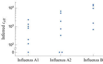
Figure S6: Inferring $c_{\text{eff}}$ between every tethered construct binding to each group of influenza virus. The best-fit effective concentration of $\text{Ab}_{\text{A1}}\text{\textendash}\text{Ab}_{\text{A2}}$ against the influenza A group 1 and group 2 strains, together with the effective concentration of $\text{Ab}_{\text{B}}^{(1)}\text{\textendash}\text{Ab}_{\text{B}}^{(2)}$ binding to influenza B.

References

- 1. Awwad S, Angkawinitwong U. Overview of Antibody Drug Delivery. Pharmaceutics. 2018;10(3):83. doi:10.3390/pharmaceutics10030083.
- 2. Caskey M, Klein F, Nussenzweig MC. Broadly neutralizing anti-HIV-1 monoclonal antibodies in the clinic. Nature Medicine. 2019;25(4):547–553. doi:10.1038/s41591-019-0412-8.
- 3. Perelson AS, Weisbuch G. Immunology for physicists. Reviews of Modern Physics. 1997;69(4):1219–1268. doi:10.1103/RevModPhys.69.1219.
- 4. Mukherjee S. The emperor of all maladies: A biography of cancer. Scribner; 2010.
- 5. Chow SK, Smith C, MacCarthy T, Pohl MA, Bergman A, Casadevall A. Disease-enhancing antibodies improve the efficacy of bacterial toxin-neutralizing antibodies. Cell Host & Microbe. 2013;13(4):417–28. doi:10.1016/j.chom.2013.03.001.
- 6. Koefoed K, Steinaa L, Soderberg JN, Kjaer I, Jacobsen HJ, Meijer PJ, et al. Rational identification of an optimal antibody mixture for targeting the epidermal growth factor receptor. mAbs. 2011;3(6):584–595. doi:10.4161/mabs.3.6.17955.
- 7. Laursen NS, Friesen RHE, Zhu X, Jongeneelen M, Blokland S, Vermond J, et al. Universal protection against influenza infection by a multidomain antibody to influenza hemagglutinin. Science. 2018;362(6414):598–602. doi:10.1126/science.aaq0620.
- 8. Spiess C, Zhai Q. Alternative molecular formats and therapeutic applications for bispecific antibodies. Molecular Immunology. 2015;67(2):95–106. doi:10.1016/J.MOLIMM.2015.01.003.
- 9. Knossow M, Gaudier M, Douglas A, Barrère B, Bizebard T, Barbey C, et al. Mechanism of Neutralization of Influenza Virus Infectivity by Antibodies. Virology. 2002;302(2):294–298. doi:10.1006/VIRO.2002.1625.
- 10. Ndifon W, Wingreen NS, Levin SA. Differential Neutralization Efficiency of Hemagglutinin Epitopes, Antibody Interference, and the Design of Influenza Vaccines. Proceedings of the National Academy of Sciences of the United States of America. 2009;106(21):8701–6. doi:10.1073/pnas.0903427106.
- 11. Einav T, Yazdi S, Coey A, Bjorkman PJ, Phillips R. Harnessing Avidity: Quantifying Entropic and Energetic Effects of Linker Length and Rigidity Required for Multivalent Binding of Antibodies to HIV-1 Spikes. bioRxiv. 2019; p. 406454. doi:10.1101/406454.
- 12. Kong R, Louder MK, Wagh K, Bailer RT, DeCamp A, Greene K, et al. Improving neutralization potency and breadth by combining broadly reactive HIV-1 antibodies targeting major neutralization epitopes. Journal of virology. 2015;89(5):2659–71. doi:10.1128/JVI.03136-14.
- 13. Palmer AC, Sorger PK. Combination Cancer Therapy Can Confer Benefit via Patient-to-Patient Variability without Drug Additivity or Synergy. Cell. 2017;171(7):1678–1691.e13. doi:10.1016/J.CELL.2017.11.009.
- 14. Klein JS, Jiang S, Galimidi RP, Keeffe JR, Bjorkman PJ, Regan L. Design and characterization of structured protein linkers with differing flexibilities. Protein Engineering, Design and Selection. 2014;27(10):325–330. doi:10.1093/protein/gzu043.
- 15. Rohatgi A. WebPlotDigitizer; 2017. Available from: https://automeris.io/WebPlotDigitizer.
- 16. Bintu L, Buchler NE, Garcia HG, Gerland U, Hwa T, Kondev J, et al. Transcriptional regulation by the numbers: models. Current Opinion in Genetics & Development. 2005;15(2):116–124. doi:10.1016/j.gde.2005.02.007.
- 17. Xu H, Shaw DE. A Simple Model of Multivalent Adhesion and Its Application to Influenza Infection. Biophysical Journal. 2016;110(1):218–233. doi:10.1016/j.bpj.2015.10.045.
- 18. Klasse PJ, Sattentau QJ. Occupancy and Mechanism in Antibody-Mediated Neutralization of Animal Viruses. Journal of General Virology. 2002;83(9):2091–2108. doi:10.1099/0022-1317-83-9-2091.
- 19. Klein JS, Bjorkman PJ. Few and Far Between: How HIV May Be Evading Antibody Avidity. PLoS Pathogens. 2010;6(5):e1000908. doi:10.1371/journal.ppat.1000908.
- 20. Brandenberg OF, Magnus C, Rusert P, Günthard HF, Regoes RR, Trkola A. Predicting HIV-1 transmission and antibody neutralization efficacy in vivo from stoichiometric parameters. PLoS Pathogens. 2017;13(5):1–35. doi:10.1371/journal.ppat.1006313.