Uncertainty Quantification for Bayesian CART

Supplement to “Uncertainty Quantification for Bayesian CART”

Abstract

This work affords new insights into Bayesian CART in the context of structured wavelet shrinkage. The main thrust is to develop a formal inferential framework for Bayesian tree-based regression. We reframe Bayesian CART as a $g$-type prior which departs from the typical wavelet product priors by harnessing correlation induced by the tree topology. The practically used Bayesian CART priors are shown to attain adaptive near rate-minimax posterior concentration in the supremum norm in regression models. For the fundamental goal of uncertainty quantification, we construct adaptive confidence bands for the regression function with uniform coverage under self-similarity. In addition, we show that tree-posteriors enable optimal inference in the form of efficient confidence sets for smooth functionals of the regression function.

Abstract

This supplementary file contains additional material, including results for nonparametric regression, a simulation study, an adaptive nonparametric Bernstein–von Mises theorem, and details on tensor–multivariate versions of the considered prior distributions. It also contains all remaining proofs for the results stated in the main paper.

t1The author gratefully acknowledges support from the Institut Universitaire de France and from the ANR grant ANR-17-CE40-0001 (BASICS). t2 The author gratefully acknowledges support from the James S. Kemper Foundation Faculty Research Fund at the University of Chicago Booth School of Business and the National Science Foundation (grant DMS-1944740).

1 Introduction

The widespread popularity of Bayesian tree-based regression has raised considerable interest in theoretical understanding of their empirical success. However, theoretical literature on methods such as Bayesian CART and BART is still in its infancy. In particular, statistical inferential theory for regression trees and forests (both frequentist and Bayesian) has been severely under-developed.

This work sheds light on Bayesian CART [22, 25] which is a popular learning tool based on ideas of recursive partitioning and which forms an integral constituent of BART [21]. Bayesian Additive Regression Trees (also known as BART) have emerged as one of today’s most effective general approaches to predictive modeling under minimal assumptions. Their empirical success has been amply illustrated in the context of non-parametric regression [21], classification [49], variable selection [8, 48, 46], shape constrained inference [20], causal inference [41, 40], to name a few. The BART model deploys an additive aggregate of individual trees using Bayesian CART as its building block. While theory for random forests, the frequentist counterpart, has seen numerous recent developments [64, 6, 56, 44, 63], theory for Bayesian CART and BART has not kept pace with its application. With the first theoretical results (Hellinger convergence rates) emerging very recently [55, 47, 54], many fundamental questions pertaining to, e.g., convergence in stronger losses such as the supremum norm, as well as uncertainty quantification (UQ), have remained to be addressed. This work takes a leap forward in this important direction by developing a formal frequentist statistical framework for uncertainty quantification with confidence bands for Bayesian CART.

We first show that Bayesian CART reaches a (near-)optimal posterior convergence rate under the supremum-norm loss, a natural loss for UQ of regression functions. Many methods that are adaptive for the $L^{2}$–loss actually fail to be adaptive in an $L^{\infty}$–sense, as we illustrate below. We are actually not aware of any sharp supremum-norm convergence rate result for related machine learning methods in the literature, including CART, random forests and deep learning. Regarding inference, we provide a construction of an adaptive credible band for the unknown regression function with (nearly, up a to logarithmic term) optimal uniform coverage under self-similarity. In addition, we provide efficient confidence sets and bands for a family of smooth functionals. Uncertainty quantification for related random forests or deep learning has been an open problem, with distributional results available only for point-wise prediction using bootstrap techniques [44]. Our results make a needed contribution to the literature on the widely sought-after UQ for (tree-based) machine learning methods.

Regarding supremum-norm (and its associated discrete $\ell_{\infty}$ version) posterior contraction rates, their derivation is typically more delicate compared to the more familiar testing distances (e.g. $L^{2}$ or Hellinger) for which general theory has been available since the seminal work [34]. Despite the lack of unifying theory, however, advances have been made in the last few years [36, 14, 43] including specific models [58, 70, 51, 52]. However, Bayesian adaptation for the supremum loss has been obtained, to the best of our knowledge, only through spike-and-slab priors (the work [69] uses Gaussian process priors, but adaptation is obtained via Lepski’s method). In particular, [43] show that spike-and-slab priors on wavelet coefficients yield the exact adaptive minimax rate in the white noise model and [67] considers the anisotropic case in a regression framework. For density estimation, [15, 16] derive optimal $\|\cdot\|_{\infty}$–rates for Pólya tree priors, while [50] considers adaptation for log-density spike and slab priors. In this work, we consider Gaussian white noise and non-parametric regression with Bayesian CART which is widely used in practice.

Bayesian CART is a method of function estimation based on ideas of recursive partitioning of the predictor space. The work [28] highlighted the link between dyadic CART and best ortho-basis selection using Haar wavelets in two dimensions; [32] furthered this connection by considering unbalanced Haar wavelets of [38]. CART methods have been also studied in the machine learning literature, see e.g. [7, 57, 65] and references therein. Unlike plain wavelet shrinkage methods and standard spike-and-slab priors, general Bayesian CART priors have extra flexibility by allowing for (some) basis selection. First results in this direction are derived in Section 4. This aspect is particularly useful in higher-dimensional data, where CART methods have been regarded as an attractive alternative to other methods [29].

By taking the Bayesian point of view, we relate Bayesian CART to structured wavelet shrinkage using libraries of weakly balanced Haar bases. Each tree provides an underlying skeleton or a ‘sparsity structure’ which supervises the sparsity pattern (see e.g. [2]). We show that Bayesian CART borrows strength between coefficients in the tree ancestry by giving rise to a variant of the $g$-prior [71]. Similarly as independent product priors, we show that these dependent priors also lead to adaptive supremum norm concentration rates (up to a logarithmic factor). To illustrate that local (internal) sparsity is a key driver of adaptivity, we show that dense trees are incapable of adaptation.

To convey the main ideas, the mathematical development will be performed through the lense of a Gaussian white noise model. Our techniques, however, also apply in non-parametric regression. Results in this setting are briefly presented in Section 3.5 with details postponed until the Supplement (Section 7.1). The white noise model is defined through the following stochastic differential equation, for an integer $n\geq 1$,

$$dX(t)=f_{0}(t)dt+\frac{1}{\sqrt{n}}dW(t),\quad t\in[0,1],$$ (1)

where $X(t)$ is an observation process, $W(t)$ is the standard Wiener process on $[0,1]$ and $f_{0}$ is unknown and belongs to $L^{2}[0,1]$, set of squared–integrable functions on $[0,1]$. The model (1) is observationally equivalent to a Gaussian sequence space model after projecting the observation process onto a wavelet basis $\{\psi_{lk}:l\geq 0,0\leq k\leq 2^{l}-1\}$ of $L^{2}[0,1]$. This sequence model writes as

$$X_{lk}=\beta_{lk}^{0}+\frac{\varepsilon_{lk}}{\sqrt{n}},\qquad\varepsilon_{lk}\stackrel{{\scriptstyle iid}}{{\sim}}\mathcal{N}(0,1),$$ (2)

where the wavelet coefficients $\beta_{lk}^{0}=\langle f_{0},\psi_{lk}\rangle=\int_{0}^{1}f_{0}(t)\psi_{lk}(t)dt$ of $f_{0}$ are indexed by a scale index $l\geq-1$ and a location index $k\in\{0,\ldots,(2^{l}-1)_{+}\}$. A paradigmatic example is the standard Haar wavelet basis

$$\psi_{-10}(x)=\mathbb{I}_{[0,1]}(x)\quad\text{and}\quad\psi_{lk}(x)=2^{l/2}\psi(2^{l}x-k)\quad(l\geq 0),$$ (3)

obtained with orthonormal dilation-translations of $\psi=\mathbb{I}_{(0,1/2]}-\mathbb{I}_{(1/2,1]}$, where $\mathbb{I}_{A}$ denotes the indicator of a set $A$. Later in the text, we also consider weakly balanced Haar wavelet relaxations (Section 4), as well as smooth wavelet bases (Section 10.2).

One of the key motivations behind the Bayesian approach is the mere fact that the posterior is an actual distribution, whose limiting shape can be analyzed towards obtaining uncertainty quantification and inference. Our results in this direction can be grouped in two subsets. First, for uncertainty quantification for $f_{0}$ itself, we construct adaptive and honest confidence bands under self-similarity (with coverage converging to one). Exact asymptotic coverage is achieved through intersections with a multiscale credible band (along the lines of [53]). Confidence bands construction for regression surfaces is a fundamental task in nonparametric regression and can indicate whether there is empirical evidence to support conjectured features such as multi-modality or exceedance of a level. Results of this type are, to date, unavailable for classical CART, random forests and/or deep learning. Second, we consider inference for smooth functionals of $f_{0}$, including linear ones and the primitive functional $\int_{0}^{\cdot}f_{0}$, for which exact optimal confidence sets are derived from posterior quantiles. While these results for functionals are stated in the main paper (Theorem 4 below), their derivation is most naturally obtained through a general limiting shape result, stated and proved in the Supplement (Theorem 9). Such an adaptive Bernstein-von Mises theorem for Bayesian CART is obtained following the approach of [17, 18]; it is only the second result of this kind (providing adaptation) after the recent result of Ray [53].

The paper is structured as follows. Section 2 introduces regression tree-priors, as well as the notion of tree-shaped sparsity and the $g$-prior for trees. In Section 3, we state supremum-norm inference properties of Bayesian dyadic CART (estimation and confidence bands). Section 4 considers flexible partitionings allowing for basis choice. A brief discussion can be found in Section 5. The proof of our master Theorem 1 can be found in Section 6. The supplementary file [19] gathers the proofs of the remaining results. The sections and equations of this supplement are referred to with an additional symbol “S-” in the numbering.

Notation. Let $\mathcal{C}([0,1])$ denote the set of continuous functions on $[0,1]$ and let $\phi_{\sigma}$ denote the normal density with zero mean and variance $\sigma^{2}$. Let $\mathbb{N}=\{0,1,2,\ldots\}$ be the set of natural integers and $\mathbb{N}^{*}=\mathbb{N}\setminus\{0\}$. We denote by $I_{K}$ the $K\times K$ identity matrix, Also, $B^{c}$ denotes the complement of a set $B$. For an interval $I=(a,b]\subset(0,1]$, let $|I|=b-a$ be its diameter and $a\vee b=\max(a,b)$. The notation $x\lesssim y$ means $x\leq Cy$ for $C$ a large enough universal constant, and $:=$ (or $=:$) means “the left-hand side is defined as”.

2 Trees and Wavelets

In this section, we discuss multiscale prior assignments on functions $f\in L^{2}[0,1]$ (i.e. priors on the sequence of wavelet coefficients $\beta_{lk}={\langle}f,\psi_{lk}{\rangle})$ inspired by (and including) Bayesian CART. Such methods recursively subdivide the predictor space into cells where $f$ can be estimated locally. The partitioning process can be captured with a tree object (a hierarchical collection of nodes) and a set of splitting rules attached to each node. Section 2.1 discusses priors on the tree object. The splitting rules are ultimately tied to a chosen basis, where the traditional Haar wavelet basis yields deterministic dyadic splits (as we explain in Section 2.1.2). Later in Section 4, we extend our framework to random unbalanced Haar bases which allow for more flexible splits. Beyond random partitioning, an integral component of CART methods are histogram heights assigned to each partitioning cell. We flesh out connections between Bayesian histograms and wavelets in Section 2.2. Finally, we discuss Bayesian CART priors over histogram heights in Section 2.3.

2.1 Priors on Trees $\Pi_{\mathbb{T}}(\cdot)$

First, we need to make precise our definition of a tree object which will form a skeleton of our prior on $(\beta_{lk})$ for each given basis $\{\psi_{lk}\}$. Throughout this paper, we will largely work with the Haar basis.

Definition 1 (Tree terminology).

We define a binary tree $\mathcal{T}$ as a collection of nodes $(l,k)$, where $l\in\mathbb{N},\,k\in\{0,\dots,2^{l}-1\}$, that satisfies

$$(l,k)\in\mathcal{T},\,l\geq 1\ \Rightarrow\ (l-1,\lfloor k/2\rfloor)\in\mathcal{T}.$$

In the last display, the node $(l,k)$ is a child of its parent node $(l-1,\lfloor k/2\rfloor)$. A full binary tree consists of nodes with exactly $0$ or $2$ children. For a node $(l,k)$, we refer to $l$ as the layer index (or also depth) and $k$ as the position in the $l^{th}$ layer (from left to right). The cardinality $|\mathcal{T}|$ of a tree $\mathcal{T}$ is its total number of nodes and the depth is defined as $d(\mathcal{T})=\max\limits_{(l,k)\in\mathcal{T}}l$.

A node $(l,k)\in\mathcal{T}$ belongs to the set $\mathcal{T}_{ext}$ of external nodes (also called leaves) of $\mathcal{T}$ if it has no children and to the set $\mathcal{T}_{int}$ of internal nodes, otherwise. By definition $|\mathcal{T}|=|\mathcal{T}_{int}|+|\mathcal{T}_{ext}|$, where, for full binary trees, we have $|\mathcal{T}|=2|\mathcal{T}_{int}|+1$. An example of a full binary tree is depicted in Figure 1(a). In the sequel, $\mathbb{T}$ denotes the set of full binary trees of depth no larger than $L=L_{max}=\lfloor\log_{2}n\rfloor$, a typical cut-off in wavelet analysis. Indeed, trees can be associated with certain wavelet decompositions, as will be seen in Section 2.2.2.

Before defining tree-structured priors over the entire functions $f$’s, we first discuss various ways of assigning a prior distribution over $\mathbb{T}$, that is over trees themselves. We focus on the Bayesian CART prior [22], which became an integral component of many Bayesian tree regression methods including BART [21].

2.1.1 Bayesian CART Priors

The Bayesian CART construction of [22] assigns a prior over $\mathbb{T}$ via the heterogeneous Galton-Watson (GW) process. The prior description utilizes the following top-down left-to-right exploration metaphor (see also [54]). Denote with $Q$ a queue of nodes waiting to be explored. Each node $(l,k)$ is assigned a random binary indicator $\gamma_{lk}\in\{0,1\}$ for whether or not it is split. Starting with ${{\mathcal{T}}}=\emptyset$, one initializes the exploration process by putting the root node $(0,0)$ tentatively in the queue, i.e. $Q=\{(0,0)\}$. One then repeats the following three steps until $Q=\emptyset$:

• Pick a node $(l,k)\in Q$ with the highest priority (i.e. the smallest index $2^{l}+k$) and if $l<L_{max}$, split it with probability

  $$p_{lk}=\mathbb{P}(\gamma_{lk}=1).$$ (4)

  If $l=L_{max}$, set $\gamma_{lk}=0$.

• If $\gamma_{lk}=0$, remove $(l,k)$ from $Q$.

• If $\gamma_{lk}=1$, then

  • add $(l,k)$ to the tree, i.e. ${{\mathcal{T}_{int}}}{\,\leftarrow\,}{{\mathcal{T}_{int}}}\cup\{(l,k)\},$

  • remove $(l,k)$ from $Q$ and if $l<L_{max}$ add its children to $Q$, i.e.

    $$Q{\ \leftarrow\ }Q\backslash\{(l,k)\}\cup\{(l+1,2k),(l+1,2k+1)\}.$$

The tree skeleton is probabilistically underpinned by the cut probabilities $(p_{lk})$ which are typically assumed to decay with the depth $l$ as a way to penalise too complex trees. While [22] suggest $p_{lk}=\alpha/(1+l)^{\gamma}$ for some $\alpha\in(0,1)$ and $\gamma>0$, [54] point out that this decay may not be fast enough and suggest instead $p_{lk}=\Gamma^{-l}$ for some $2<\Gamma<n$, which leads to a (near) optimal empirical $L^{2}$–convergence rate. We use a similar assumption in our analysis, and also assume that the split probability depends only on $l$, and simply denote $p_{l}=p_{lk}$.

Independently of [22], [25] proposed another variant of Bayesian CART, which first draws the number of leaves (i.e. external nodes) $K=|\mathcal{T}_{ext}|$ at random from a certain prior on integers, e.g. a Poisson distribution (say, conditioned to be non-zero). Then, a tree $\mathcal{T}$ is sampled uniformly at random from all full binary trees with $K$ leaves. Noting that there are $\mathbb{C}_{K-1}$ such trees, with $\mathbb{C}_{K}$ the $K$–th Catalan number (see Lemma 6), this leads to $\Pi(\mathcal{T})=(\lambda^{K}/[K!(e^{\lambda}-1)])\cdot\mathbb{C}_{K-1}^{-1}$. As we restrict to trees in $\mathbb{T}$, i.e. with depth at most $L=L_{max}$, we slightly update the previous prior choice by setting, for some $\lambda>0$, with $K=|\mathcal{T}_{ext}|$,

$$\Pi_{\mathbb{T}}(\mathcal{T})\propto\frac{\lambda^{K}}{(\mathrm{e}^{\lambda}-1)K!}\frac{1}{\mathbb{C}_{K-1}}\,\mathbb{I}_{\mathcal{T}\in\mathbb{T}},$$ (5)

where $\propto$ means ‘proportional to’. We call the resulting prior $\Pi_{\mathbb{T}}$ the ‘conditionally uniform prior’ with a parameter $\lambda$.

(a) A full binary tree

(b) Binary tree of prior cut probabilities

Figure 1: (Left) A full binary tree $\mathcal{T}=\mathcal{T}_{int}\cup\mathcal{T}_{ext}$. Red nodes are external nodes $\mathcal{T}_{ext}$ and blue nodes are internal nodes $\mathcal{T}_{int}$. (Right) A binary tree of cut probabilities $p_{lk}$ in (4).

2.1.2 Trees and Random Partitions

Trees provide a structured framework for generating random partitions of the predictor space (here we choose $(0,1]$ for simplicity of exposition). In CART methodology, each node $(l,k)\in\mathcal{T}$ is associated with a partitioning interval $I_{lk}\subseteq(0,1]$. Starting from the trivial partition $I_{00}=(0,1]$, the simplest way to obtain a partition is by successively dividing each $I_{lk}$ into $I_{lk}=I_{l+1\,2k}\cup I_{l+1\,2k+1}$. One central example is dyadic intervals $I_{lk}$ which correspond to the domain of the balanced Haar wavelets $\psi_{lk}$ in (3), i.e.

$$I_{00}=(0,1],\quad I_{lk}=(k2^{-l},(k+1)2^{-l}]\quad\text{for $l\geq 0$ and $0\leq k<2^{l}$}.$$ (6)

For any fixed depth $l\in\mathbb{N}$, the intervals $\cup_{0\leq k<2^{l}}I_{lk}$ form a deterministic regular (equispaced) partition of $(0,1]$. Trees, however, generate more flexible partitions $\cup_{(l,k)\in\mathcal{T}_{ext}}I_{lk}$ by keeping only those intervals $I_{lk}$ attached to the leaves of the tree. Since $\mathcal{T}$ is treated as random with a prior $\Pi_{\mathbb{T}}$ (as defined in Section 2.1), the resulting partition will also be random.

Example 1.

Figure 1(a) shows a full binary tree $\mathcal{T}=\mathcal{T}_{int}\cup\mathcal{T}_{ext}$, where $\mathcal{T}_{int}=\{(0,0),(1,1),(2,2)\}$ and $\mathcal{T}_{ext}=\{(1,0),(2,3),(3,4),(3,5)\},$ resulting in the partition of $(0,1]$ given by

$$(I_{lk})_{(l,k)\in\mathcal{T}_{ext}}=\{(0,1/2],(1/2,5/8],(5/8,3/4],(3/4,1]\}.$$ (7)

The set of possible split points obtained with (6) is confined to dyadic rationals. One can interpret the resulting partition as the result of recursive splitting where, at each level $l$, intervals $I_{lk}$ for each internal node $(l,k)\in\mathcal{T}_{int}$ are cut in half and intervals $I_{lk}$ for each external node $(l,k)\in\mathcal{T}_{ext}$ are left alone. We will refer to such a recursive splitting process as dyadic CART. There are several ways to generalize this construction, for instance by considering arbitrary splitting rules that iteratively dissect the intervals at values other than the midpoint. We explore such extensions in Section 4.

2.2 Tree-shaped Priors on $f$

This section outlines two strategies for assigning a tree-shaped prior distribution on $f$ underpinned by a tree skeleton $\mathcal{T}\in\mathbb{T}$. Each tree $\mathcal{T}=\mathcal{T}_{int}\cup\mathcal{T}_{ext}$ can be associated with two sets of coefficients: (a) internal coefficients $\beta_{lk}$ attached to wavelets $\psi_{lk}$ for $(l,k)\in\mathcal{T}_{int}$ and (b) external coefficients $\widetilde{\beta}_{lk}$ attached to partitioning intervals $I_{lk}$ for $(l,k)\in\mathcal{T}_{ext}$ (see Section 2.1.2). While wavelet priors (Section 2.2.1) assign the prior distribution internally on $\beta_{lk}$, Bayesian CART priors [22, 25] (Section 2.2.2) assign the prior externally on $\widetilde{\beta}_{lk}$. We discuss and relate these two strategies in more detail below.

2.2.1 Tree-shaped Wavelet Priors

Traditional (linear) Haar wavelet reconstructions for $f$ deploy all wavelet coefficients $\beta_{lk}$ with resolutions $l$ smaller than some $d>0$. This strategy amounts to fitting a flat tree with $d$ layers (i.e. a tree that contains all nodes up to a level $d$, see Figure 2) or, equivalently, a regular dyadic regression histogram with $2^{d}$ bins. This construction can be made more flexible by selecting coefficients prescribed by trees that are not necessarily flat. Given a full binary tree $\mathcal{T}\in\mathbb{T}$, one can build the following wavelet reconstruction of $f$ using only active wavelet coefficients that are inside a tree $\mathcal{T}$

$$f_{\mathcal{T},\boldsymbol{\beta}}(x)=\beta_{-10}\psi_{-10}(x)+\sum_{(l,k)\in\mathcal{T}_{int}}\beta_{lk}\psi_{lk}(x)=\sum_{(l,k)\in\mathcal{T}_{int}^{\prime}}\beta_{lk}\psi_{lk}(x),$$ (8)

where $\boldsymbol{\beta}=(\beta_{-10},(\beta_{lk})_{0\leq l\leq L-1,0\leq k<2^{l}})^{\prime}$ is a vector of wavelet coefficients and where $\mathcal{T}_{int}^{\prime}=\mathcal{T}_{int}\cup\{(-1,0)\}$ is the ‘rooted’ tree with the index $(-1,0)$ added to $\mathcal{T}_{int}$. Note that $|\mathcal{T}_{int}^{\prime}|=|\mathcal{T}_{ext}|$.

Define a tree-shaped wavelet prior on $f_{\mathcal{T},\boldsymbol{\beta}}$ as the prior induced by the hierarchical model

$$\mathcal{T}\qquad \sim\qquad\ \Pi_{\mathbb{T}}$$

$$(\beta_{lk})_{lk}\,|\>\mathcal{T}\ \sim\,\bigotimes_{(l,k)\in\mathcal{T}_{int}^{\prime}}\pi(\beta_{lk})\ \otimes\ \bigotimes_{(l,k)\notin\mathcal{T}_{int}^{\prime}}\delta_{0}(\beta_{lk}),$$ (9)

where $\Pi_{\mathbb{T}}$ is a prior on trees as described in Section 2.1.1 and where the active wavelet coefficients $\beta_{lk}$ for $(l,k)\in\mathcal{T}_{int}$ follow a distribution with a bounded and positive density $\pi(\beta_{lk})$ on $\mathbb{R}$. The prior (9) is seen as a distribution on $\mathbb{R}^{2^{L}}$, where all remaining coefficients, i.e. ${\beta_{lk}}$’s for $l\geq L$, are set to $0$.

The prior (9) contains the so-called sieve priors [18] (i.e. flat trees) as a special case, where the sieve is with respect to the approximating spaces $\text{Vect}\{\psi_{lk},l<d\}$ for some $d\geq 0$. For nonparametric estimation of $f_{0}$, it is well-known that sieve priors can achieve (nearly) adaptive rates in the $L^{2}$–sense (see e.g. [35]). In turns out, however, that sieve priors (and therefore flat tree priors) are too rigid to enable adaptive results for stronger losses such as the supremum norm, as we demonstrate in Theorem 5 in Section 3.4 (Supplement). This theorem illustrates that supremum norm adaptation using Bayesian (or other likelihood-based) methods is a delicate phenomenon that is not attainable by many typical priors.

By definition, the prior (9) weeds out all wavelet coefficients $\beta_{lk}$ that are not supported by the tree skeleton (i.e. are not internal nodes in $\mathcal{T}$). This has two shrinkage implications: global and local. First, the global level of truncation (i.e. the depth of the tree) in (9) is not fixed but random. Second, unlike in sieve priors, only some low resolution coefficients are active depending on whether or not the tree splits the node $(l,k)$. These two shrinkage aspects create hope that tree-shaped wavelet priors (9) attain adaptive supremum norm rates (up to log factors) and enable construction of adaptive confidence bands. We see later in Section 3 that this optimism is indeed warranted.

For adaptive wavelet shrinkage, [23] propose a Gaussian mixture spike-and-slab prior on the wavelet coefficients. The point mass spike-and-slab incarnation of this prior was studied by [43] and [53]. Independently for each wavelet coefficient $\beta_{lk}$ at resolutions larger than some $l_{0}(n)$ (strictly increasing sequence), the prior in [53] can be written in the standard spike-and-slab form

$$\pi(\beta_{lk}\,|\>\gamma_{lk}) =\gamma_{lk}\pi(\beta_{lk})+(1-\gamma_{lk})\delta_{0}(\beta_{lk}),$$ (10)

where $\gamma_{lk}\in\{0,1\}$ for whether or not the coefficient is active with $\mathbb{P}(\gamma_{lk}=1\,|\>\theta_{l})=\theta_{l}$. Moreover, the prior on all coefficients at resolutions no larger than $l_{0}(n)$ is dense, i.e. $\theta_{l}=1$ for $l\leq l_{0}(n)$. The value $\theta_{l}$ can be viewed as the probability that a given wavelet coefficient $\beta_{lk}$ at resolution $l$ will contain ‘signal’.

There are undeniable similarities between (9) and (10), in the sense that the binary inclusion indicator $\gamma_{lk}$ in (10) can be regarded as the node splitting indicator $\gamma_{lk}$ in (4). While the indicators $\gamma_{lk}$ in (10) are independent under the spike-and-slab prior, they are hierarchically constrained under the CART prior, where the pattern of non-zeroes encodes the tree oligarchy. The seeming resemblance of the CART-type prior (9) to the spike-and-slab prior (10) makes one naturally wonder whether, unlike sieve-type priors, CART posteriors attain adaptive supremum-norm inference.

2.2.2 Bayesian CART Priors

A perhaps more transparent approach to assigning a tree-shaped prior on $f$ is through histograms (as opposed to wavelet reconstructions from Section 2.2.1). Each tree $\mathcal{T}\in\mathbb{T}$ generates a random partition via intervals $I_{lk}$ (see Section 2.1.2) and gives rise to the following histogram representation

$$\widetilde{f}_{\mathcal{T},\widetilde{\boldsymbol{\beta}}}(x)=\sum_{(l,k)\in\mathcal{T}_{ext}}\widetilde{\beta}_{lk}\mathbb{I}_{I_{lk}}(x),$$ (11)

where ${\widetilde{\boldsymbol{\beta}}}=(\widetilde{\beta}_{lk}:(l,k)\in\mathcal{T}_{ext})^{\prime}$ is a vector of reals interpreted as step heights and where $I_{lk}$’s are obtained from the tree $\mathcal{T}$ as in Section 2.1.2 (and as illustrated in Example 1). We now define the (Dyadic) Bayesian CART prior on $f$ using the following hierarchical model on the external coefficients rather than internal coefficients (compare with (9))

$$\mathcal{T}\qquad \sim\qquad\Pi_{\mathbb{T}}$$

$$(\widetilde{\beta}_{lk})_{(l,k)\in\mathcal{T}_{ext}}\,\,|\>\,\mathcal{T}\ \sim\,\bigotimes_{(l,k)\in\mathcal{T}_{ext}}{\widetilde{\pi}}(\widetilde{\beta}_{lk}),$$ (12)

where $\Pi_{\mathbb{T}}$ is as in Section 2.1, and where the height $\widetilde{\beta}_{lk}$ at a specific $(l,k)\in\mathcal{T}_{ext}$ has a bounded and positive density $\widetilde{\pi}(\widetilde{\beta}_{lk})$ on $\mathbb{R}$. This model coincides with the widely used Bayesian CART priors using a midpoint dyadic splitting rule (as we explained in Section 2.1.2). In practice, the density $\widetilde{\pi}$ is often chosen as centered Gaussian with some variance $\sigma^{2}>0$ [22, 25].

Figure 2: Flat tree with edges weighted by the amplitude of the Haar wavelets.

The histogram prior (11) can be rephrased in terms of wavelets. Indeed, the histogram representation (11) can be rewritten in terms of the internal coefficients, i.e. $\widetilde{f}_{\mathcal{T},\widetilde{\boldsymbol{\beta}}}(x)=f_{\mathcal{T},\boldsymbol{\beta}}(x)$ as in (8), with $\beta_{lk}$’s and $\widetilde{\beta}_{lk}$’s linked via

$$\widetilde{\beta}_{lk}=\beta_{-10}+\sum_{j=0}^{l-1}s_{\lfloor k/2^{l-j-1}\rfloor}2^{j/2}\beta_{j\lfloor k/2^{l-j}\rfloor},$$ (13)

where $s_{k}=(-1)^{k+1}$. The identity (13) follows the fact that for $x\in I_{lk}$ we obtain $\widetilde{\beta}_{lk}=\sum_{(l^{\prime},k^{\prime})\in P_{lk}}\beta_{l^{\prime}k^{\prime}}\psi_{l^{\prime}k^{\prime}}$ from (11), where $P_{lk}\equiv\{(j,\lfloor k/2^{l-j}\rfloor):j=0,\dots,l-1\}$ are the ancestors of the bottom node $(l,k)$. Note that $\psi_{j\lfloor k/2^{l-j}\rfloor}=2^{j/2}s_{\lfloor k/2^{l-j-1}\rfloor}$ where $s=(-1)^{k+1}$ for whether $x$ belongs to the left (positive sign) or right (negative sign) of the wavelet piece. There is a pinball game metaphor behind (13). A ball is dropped through a series of dyadically arranged pins of which the ball can bounce off to the right (when $s_{k}=+1$) or to the left (when $s_{k}=-1$). The ball ultimately lands in one of the histogram bins $I_{lk}$ whose coefficient $\widetilde{\beta}_{lk}$ is obtained by aggregating $\beta_{lk}$’s of those pins $(l,k)$ that the ball encountered on its way down. The pinball aggregation process can be understood from Figure 3. The duality between the equivalent representations (11) and (8) through (13) provides various avenues for constructing prior distributions, and enables an interesting interpretation of Bayesian CART [22, 25] as a correlated wavelet prior, as we now see.

2.3 The $g$-prior for Trees

We now discuss various ways of assigning a prior distribution on the bottom node histogram heights $\widetilde{\beta}_{lk}$ and, equivalently, the internal Haar wavelet coefficients $\beta_{lk}$. This section also describes an interesting connection between the widely used Bayesian CART prior [22, 25] and a $g$-prior [71] on wavelet coefficients. For a given tree $\mathcal{T}$, let $\boldsymbol{\beta}_{\mathcal{T}}=(\beta_{lk}:(l,k)\in\mathcal{T}_{int}^{\prime})^{\prime}$ denote the vector of ordered internal node coefficients $\beta_{lk}$ including the extra root node $(-1,0)$ (and with ascending ordering according to $2^{l}+k$). Similarly, $\widetilde{\boldsymbol{\beta}}_{\mathcal{T}}=(\beta_{lk}:(l,k)\in\mathcal{T}_{ext})^{\prime}$ is the vector of ordered external node coefficients $\widetilde{\beta}_{lk}$. The duality between $\boldsymbol{\beta}_{\mathcal{T}}$ and $\widetilde{\boldsymbol{\beta}}_{\mathcal{T}}$ is apparent from the pinball equation (13) written in matrix form

$$\widetilde{\boldsymbol{\beta}}_{\mathcal{T}}=A_{\mathcal{T}}\boldsymbol{\beta}_{\mathcal{T}},$$ (14)

where $A_{\mathcal{T}}$ is a square $|\mathcal{T}_{ext}|\times|\mathcal{T}_{int}^{\prime}|$ matrix (noting $|\mathcal{T}_{ext}|=|\mathcal{T}_{int}^{\prime}|$), further referred to as the pinball matrix. Each row of $A_{\mathcal{T}}$ encodes the ancestors of the external node, where the nonzero entries correspond to the internal nodes in the family pedigree. The entries are rescaled, where younger ancestors are assigned more weight. For example, the tree $\mathcal{T}$ in Figure 3(a) induces a pinball matrix $A_{\mathcal{T}}$ in Figure 3(b). The pinball matrix $A_{\mathcal{T}}$ can be easily expressed in terms of a diagonal matrix and an orthogonal matrix as

$$A_{\mathcal{T}}A_{\mathcal{T}}^{\prime}=\boldsymbol{D}_{\mathcal{T}},\quad\text{where}\quad\boldsymbol{D}_{\mathcal{T}}=\mathrm{diag}\{\widetilde{d}_{lk,lk}\}_{(l,k)\in\mathcal{T}_{ext}},\ \ \widetilde{d}_{lk,lk}=2^{l}.$$ (15)

This results from the fact that the collection $(2^{l/2}\mathbb{I}_{lk},\,(l,k)\in\mathcal{T}_{ext})$ is an orthonormal system spanning the same space as $(\psi_{jk},\,(j,k)\in\mathcal{T}_{int}^{\prime})$, so $\boldsymbol{D}_{\mathcal{T}}^{-1/2}A_{\mathcal{T}}$ is an orthonormal change–of–basis matrix. We now exhibit precise connections between the theoretical wavelet prior (9) which draws $\beta_{lk}\sim\pi$ and the practical Bayesian CART histogram prior which draws $\widetilde{\beta}_{lk}\sim{\widetilde{\pi}}$.

(a)

$$\left(\begin{matrix}\widetilde{\beta}_{11}\\ \widetilde{\beta}_{20}\\ \widetilde{\beta}_{32}\\ \widetilde{\beta}_{33}\end{matrix}\right)=\left(\begin{matrix}1&1&0&0\\ 1&-1&-\sqrt{2}&0\\ 1&-1&\sqrt{2}&-2\\ 1&-1&\sqrt{2}&2\\ \end{matrix}\right)\left(\begin{matrix}\beta_{-10}\\ \beta_{00}\\ \beta_{10}\\ \beta_{21}\end{matrix}\right)$$

(b)

Figure 3: (a) Example of a full binary tree, edges weighted by the amplitude of the Haar wavelets. (b) Pinball matrix of the tree in (a).

Recall that the wavelet prior (9) assumes independent wavelet coefficients, e.g. through the standard Gaussian prior $\boldsymbol{\beta}_{\mathcal{T}}\sim\mathcal{N}(0,I_{|\mathcal{T}_{ext}|})$. Starting from within the tree, this translates into the following independent product prior on the bottom coefficients $\widetilde{\beta}_{lk}$ through (14)

$$\widetilde{\boldsymbol{\beta}}_{\mathcal{T}}\sim\mathcal{N}(0,\boldsymbol{D}_{\mathcal{T}}),\quad\text{where}\quad\boldsymbol{D}_{\mathcal{T}}\quad\text{was defined in \eqref{eq:lemma1}},$$ (16)

i.e. $\mathrm{var}\,\widetilde{\beta}_{lk}=2^{l}$ where the variances increase with the resolution $l$.

The Bayesian CART prior [22, 25], on the other hand, starts from outside the tree by assigning $\widetilde{\boldsymbol{\beta}}_{\mathcal{T}}\sim\mathcal{N}(0,g_{n}I_{|\mathcal{T}_{ext}|})$ for some $g_{n}>0$, ultimately setting the bottom node variances equal. This translates into the following ‘$g$-prior’ on the internal wavelet coefficients through the duality (14).

Definition 2.

Let $\mathcal{T}\in\mathbb{T}$ with a pinball matrix $A_{\mathcal{T}}$ and denote with $\boldsymbol{\beta}_{\mathcal{T}}$ the internal wavelet coefficients. We define the g-prior for trees as

$$\boldsymbol{\boldsymbol{\beta}}_{\mathcal{T}} \sim\mathcal{N}\left(0,g_{n}\,(A_{\mathcal{T}}^{\prime}A_{\mathcal{T}})^{-1}\right)\quad\text{for some $g_{n}>0$}.$$ (17)

Note that, except for very special cases (e.g. flat trees) $A_{\mathcal{T}}^{\prime}A_{\mathcal{T}}$ is in general not diagonal, unlike $A_{\mathcal{T}}A_{\mathcal{T}}^{\prime}$. This means that the correlation structure induced by the Bayesian CART prior on internal wavelet coefficients is non-trivial, although $A_{\mathcal{T}}^{\prime}A_{\mathcal{T}}$ admits some partial sparsity. We characterize basic properties of the pinball matrix in Section 8.1 in the Supplement. For example, Proposition 3 shows that matrices $A_{\mathcal{T}}^{\prime}A_{\mathcal{T}}$ and $A_{\mathcal{T}}A_{\mathcal{T}}^{\prime}$ have the same eigenspectrum consisting of values $2^{l}$ where $l$ corresponds to the depth of the bottom nodes. This means that the $g$-prior variances (diagonal elements of $g_{n}(A_{\mathcal{T}}^{\prime}A_{\mathcal{T}})^{-1}$) are lower-bounded by the minimal eigenvalue of $g_{n}(A_{\mathcal{T}}^{\prime}A_{\mathcal{T}})^{-1}$ which equals $g_{n}2^{-l}$ (where $l$ is the depth of the deepest external node) which is lower-bounded by $g_{n}/n$. Since the traditional wavelet prior assumes variance $1$, the choice $g_{n}=n$ matches the lower bound $1$ by undersmoothing all possible variance combinations. While other choices could be potentially used (see [30, 45, 31] in the context of linear regression), we will consider $g_{n}=n$ in our results below.

We regard (17) as the ‘$g$-prior for trees’ due to its apparent similarity to $g$-priors for linear regression coefficients [71]. The $g$-prior has been shown to have many favorable properties in terms of invariance or predictive matching [5, 4]. Here, we explore the benefits of the $g$-type correlation structure in the context of structured wavelet shrinkage where each ‘model’ is defined by a tree topology. The correlation structure (17) makes this prior very different from any other prior studied in the context of wavelet shrinkage.

3 Inference with (Dyadic) Bayesian CART

In this section we investigate the inference properties of tree-based posteriors, showing that (a) they attain the minimax rate of posterior concentration in the supremum-norm sense (up to a log factor), and (b) enable uncertainty quantification: for $f$ in the form of adaptive confidence bands, and for smooth functionals thereof, in terms of Bernstein-von Mises type results. For clarity of exposition, we focus now on the one-dimensional case, but the results readily extend to the multi-dimensional setting with $\mathbb{R}^{d}$, $d\geq 1$ fixed, as predictor space; see Section 7.4 for more details.

3.1 Posterior supremum-norm convergence

Let us recall the standard inequality (see e.g. (60) below), for $f_{0}$ a continuous function and $f$ a Haar histogram (8), with coefficients $\beta^{0}_{lk}$ and $\beta_{lk}$,

$$\|f-f_{0}\|_{\infty}\leq|\beta_{-10}-\beta^{0}_{-10}|+\sum_{l\geq-1}2^{l/2}\max_{0\leq k<2^{l}}|\beta_{lk}-\beta^{0}_{lk}|=:\ell_{\infty}(f,f_{0}).$$ (18)

As $\ell_{\infty}$ dominates $\|\cdot\|_{\infty}$, it is enough to derive results for the $\ell_{\infty}$–loss.

Given a tree $\mathcal{T}\in\mathbb{T}$, and recalling that trees in $\mathbb{T}$ have depth at most $L:=L_{max}=\lfloor\log_{2}{n}\rfloor$, we consider a generalized tree-shaped prior $\Pi$ on the internal wavelet coefficients, recalling the notation $\mathcal{T}_{int}^{\prime}$ from Section 2.2,

$$\mathcal{T}\qquad \sim\qquad\Pi_{\mathbb{T}}$$

$$(\beta_{lk})_{l\leq L,k<2^{l}}\,|\,\mathcal{T}\ \sim\ \pi(\boldsymbol{\beta}_{\mathcal{T}})\,\otimes\bigotimes_{(l,k)\notin\mathcal{T}_{int}^{\prime}}\delta_{0}(\beta_{lk}),$$ (19)

where $\pi(\boldsymbol{\beta}_{\mathcal{T}})$ is a law to be chosen on $\mathbb{R}^{|\mathcal{T}_{int}^{\prime}|}$, not necessarily of a product form. This is a generalization of (9), which allows for correlated wavelet coefficients (e.g. the $g$-prior). Let $\boldsymbol{X}_{\mathcal{T}}$ denote the vector of ordered responses $X_{lk}$ in (2) for $(l,k)\in\mathcal{T}_{int}^{\prime}$. From the white noise model, we have

$$\boldsymbol{X}_{\mathcal{T}}=\boldsymbol{\beta}_{\mathcal{T}}+\frac{1}{\sqrt{n}}\boldsymbol{\varepsilon}_{\mathcal{T}},\quad\text{ with}\quad\boldsymbol{\varepsilon}_{\mathcal{T}}\sim\mathcal{N}(0,I_{|\mathcal{T}_{ext}|})\ \ (\text{given }\mathcal{T}).$$

By Bayes’ formula, the posterior distribution $\Pi[\cdot\,|\,X]$ of the variables $(\beta_{lk})_{l\leq L,k}$ has density

$$\sum_{\mathcal{T}\in\mathbb{T}}\Pi[\mathcal{T}\,|\>X]\cdot\pi(\boldsymbol{\beta}_{\mathcal{T}}\,|\>X)\cdot\prod_{(l,k)\notin\mathcal{T}_{int}^{\prime}}\mathbb{I}_{0}(\beta_{lk}),$$ (20)

where, denoting as shorthand $N_{X}(\mathcal{T})=\int\mathrm{e}^{-\frac{n}{2}\|\boldsymbol{\beta}_{\mathcal{T}}\|^{2}_{2}+n\boldsymbol{X}_{\mathcal{T}}^{\prime}\boldsymbol{\beta}_{\mathcal{T}}}\pi(\boldsymbol{\beta}_{\mathcal{T}})d\boldsymbol{\beta}_{\mathcal{T}}$,

$$\pi(\boldsymbol{\beta}_{\mathcal{T}}\,|\>X) =\frac{\mathrm{e}^{-\frac{n}{2}\|\boldsymbol{\beta}_{\mathcal{T}}\|^{2}_{2}+n\boldsymbol{X}_{\mathcal{T}}^{\prime}\boldsymbol{\beta}_{\mathcal{T}}}\pi(\boldsymbol{\beta}_{\mathcal{T}})}{N_{X}(\mathcal{T})},$$ (21)

$$\Pi[\mathcal{T}\,|\,X] =\frac{W_{X}(\mathcal{T})}{\displaystyle\sum_{\mathcal{T}\in\mathbb{T}}W_{X}(\mathcal{T})},\quad\text{with}\quad W_{X}(\mathcal{T})=\Pi_{\mathbb{T}}(\mathcal{T})N_{X}(\mathcal{T}).$$ (22)

Let us note that the sum in the last display is finite, as we restrict to trees of depth at most $L=L_{max}$. Note that the classes of priors $\Pi_{\mathbb{T}}$ from Section 2 are non-conjugate, i.e. the posterior on trees is given by the somewhat intricate expression (22) and does not belong to one of the classes of $\Pi_{\mathbb{T}}$ priors. While the posterior expression (21) allows for general priors $\pi(\boldsymbol{\beta}_{\mathcal{T}})$, we will focus on conditionally conjugate Gaussian priors for simplicity. This assumption is not essential and can be relaxed. For instance, in case $\pi(\boldsymbol{\beta}_{\mathcal{T}})$ is of a product form, one could use a product of e.g. Laplace distributions, using similar ideas as in [17], Theorem 5.

Our first result exemplifies the potential of tree-shaped priors by showing that Dyadic Bayesian CART achieves the minimax rate of posterior concentration over Hölder balls in the sup-norm sense, i.e. $\varepsilon_{n}=(n/\log n)^{-\alpha/(2\alpha+1)}$, up to a logarithmic term. Define a Hölder-type ball of functions on $[0,1]$ as

$$\mathcal{H}(\alpha,M):=\left\{f\in{\mathcal{C}[0,1]}:\ \max_{l\geq 0,\ 0\leq k<2^{l}}2^{l(\frac{1}{2}+\alpha)}|\langle f,\psi_{lk}\rangle|\vee|\langle f,\psi_{-10}\rangle|\leq M\right\}.$$ (23)

For balanced Haar wavelets $\psi_{lk}$ as in (3), $\mathcal{H}(\alpha,M)$ contains the a standard $\alpha$-Hölder (resp. Lipschitz when $\alpha=1$) ball of functions for any $\alpha\in(0,1]$, defined as

$$\mathcal{H}^{\alpha}_{M}:=\left\{f:\,\|f\|_{\infty}\leq M,\ \frac{|f(x)-f(y)|}{|x-y|^{\alpha}}\leq M\quad\forall x,y\in[0,1]\right\}.$$ (24)

Our master rate-theorem, whose proof can be found in Section 6, is stated below. It will be extended in various directions in the sequel.

Theorem 1.

Let $\Pi_{\mathbb{T}}$ be the Galton-Watson process prior from Section 2.1 with $p_{lk}=\Gamma^{-l}$ and $\Gamma>2e^{3}$. Consider the tree-shaped wavelet prior (19) with $\pi(\boldsymbol{\beta}_{\mathcal{T}})\sim\mathcal{N}(0,\Sigma_{\mathcal{T}})$, where $\Sigma_{\mathcal{T}}$ is either $I_{|\mathcal{T}_{int}^{\prime}|}$ or $g_{n}(A_{\mathcal{T}}^{\prime}A_{\mathcal{T}})^{-1}$ with $g_{n}=n$. Define

$$\varepsilon_{n}=\left(\frac{\log^{2}{n}}{n}\right)^{\frac{\alpha}{2\alpha+1}}\quad\text{for}\quad\alpha>0.$$ (25)

Then for any $\alpha\in(0,1]$, $M>0$, any sequence $M_{n}\to\infty$ we have for $n\rightarrow\infty$

$$\sup_{f_{0}\in\mathcal{H}(\alpha,M)}E_{f_{0}}\Pi\left[f_{\mathcal{T},\boldsymbol{\beta}}:\,\ell_{\infty}(f_{\mathcal{T},\boldsymbol{\beta}},f_{0})>M_{n}\varepsilon_{n}\,|\,X\right]\to 0.$$ (26)

By (18), the statement (26) also holds for the supremum loss $\|\cdot\|_{\infty}$.

Extension 1.

While Theorem 1 is formulated for Bayesian CART obtained with Haar wavelets, the concept of tree-shaped sparsity extends to general wavelets that give rise to smoother objects than just step functions. With $\{\psi_{lk}\}$ an $S$–regular wavelet basis on $[0,1]$, e.g. the boundary-corrected wavelet basis of [24] (see [37], Chapter 4, with adaptation of the range of indices $l$), and with $f_{0}\in\mathcal{H}(\alpha,M)$ defined in (23) for some $M>0$ and arbitrary $0<\alpha\leq S$, one indeed obtains the statement (26) by choosing $\Gamma\geq\Gamma_{0}(S)>0$ or $c\geq c_{0}>0$ large enough, see Section 10.2.

Theorem 1 encompasses both original Bayesian CART proposals for priors on bottom coefficients $\widetilde{\boldsymbol{\beta}}_{\mathcal{T}}\sim\mathcal{N}(0,I_{|\mathcal{T}_{ext}|})$ (the case $\Sigma_{\mathcal{T}}=g_{n}(A_{\mathcal{T}}A_{\mathcal{T}}^{\prime})^{-1}$ discussed in Section 2.3) as well as the mathematically slightly simpler wavelet priors $\Sigma_{\mathcal{T}}=I_{|\mathcal{T}_{ext}|}$ (discussed in Section 2.2.1). We did not fully optimize the constants in the statement; for instance, one can check that $\Gamma>2$ for the $g$-prior works. The rate $\varepsilon_{n}$ in (25) coincides with the minimax rate for the supremum norm in the white noise model up to a logarithmic factor $(\log{n})^{\frac{\alpha}{2\alpha+1}}$. We next show that this logarithmic factor is in fact real, i.e. not an artifact of the upper-bound proof. We state the results for smooth-wavelet priors, which enable to cover arbitrarily large regularities, but a similar result could also be formulated for the Haar basis.

Theorem 2.

Let $\Pi_{\mathbb{T}}$ be one of the Bayesian CART priors from Theorem 1. Consider the tree-shaped wavelet prior (19) with $\pi(\boldsymbol{\beta}_{\mathcal{T}})\sim\mathcal{N}(0,\Sigma_{\mathcal{T}})$, where $\Sigma_{\mathcal{T}}$ is $I_{|\mathcal{T}_{ext}|}$ and $\{\psi_{lk}\}$ an $S$–regular wavelet basis, $S\geq 1$. Let $\varepsilon_{n}$ be the rate defined in (25) for a given $0<\alpha\leq S$. Let the parameters of $\Pi_{\mathbb{T}}$ verify either $\Gamma\geq\Gamma_{0}(S)$ a large enough constant, or $c\geq c_{0}>0$ large enough. For any $M>0$, there exists $m>0$ such that, as $n\rightarrow\infty$,

$$\inf_{f_{0}\in\mathcal{H}(\alpha,M)}E_{f_{0}}\Pi\left[\ell_{\infty}(f_{\mathcal{T},\boldsymbol{\beta}},f_{0})\leq m\,\varepsilon_{n}\,|\,X\right]\to 0.$$ (27)

In other words, there exists a sequence of elements of $\mathcal{H}(\alpha,M)$ along which the posterior convergence rate is slower than $m\,\varepsilon_{n}$ in terms of the $\ell_{\infty}$–metric. In particular, the upper-bound rate of Theorem 1 cannot hold uniformly over $\mathcal{H}(\alpha,M)$ with a rate faster than $\varepsilon_{n}$, which shows that the obtained rate is sharp (note the reversed inequality in (27) with respect to (26); we refer to [13] for more details on the notion of posterior rate lower bound). The proof of Theorem 2 can be found in Section 10.3.

Extension 2.

Theorem 1 holds for a variety of other tree priors. This includes the conditionally uniform prior mentioned in Section 2.1.1 with $\lambda=1/n^{c}$ in (5), or an exponential-type prior $\Pi_{\mathbb{T}}(\mathcal{T})\,\propto\,\mathrm{e}^{-c|\mathcal{T}_{ext}|\log n}\mathbb{I}_{\mathcal{T}\in\mathbb{T}}$ for some $c>0$. One can also assume a general Gaussian prior on active wavelet coefficients with an unstructured covariance matrix $\Sigma_{\mathcal{T}}$ which satisfies $\lambda_{min}(\Sigma_{\mathcal{T}})\gtrsim 1/\sqrt{\log n}$ and $\lambda_{max}(\Sigma_{\mathcal{T}})\lesssim n^{a}$ for some $a>0$. Detailed proofs can be found in the Supplement (Section 10.1).

Only very few priors (actually only point mass spike-and-slab based priors, as discussed in the Introduction) were shown to attain adaptive posterior sup-norm concentration rates. Theorem 1 now certifies Dyadic Bayesian CART as one of them. The logarithmic penalty in the rate (25) reflects that Bayesian CART priors occupy the middle ground between flat trees (with only a depth cutoff) and spike-and-slab priors (with general sparsity patterns). As mentioned earlier, flat trees are incapable of supremum-norm adaptation, as we formally prove in Section 3.4. The fact that the more flexible Bayesian CART priors still achieves supremum-norm adaptation in a near-optimal way is a rather notable feature. From a more general perspective, we note that while general tools are available to derive adaptive $L^{2}$– or Hellinger–rate results in broad settings (e.g. model selection techniques, or the theory of posterior rates in [34]), deriving adaptive $L^{\infty}$–results is often obtained in a case-by-case basis; two possible techniques are wavelet thresholding (when empirical estimates of wavelet coefficients are available) and Lepski’s method (which requires some ‘ordered’ set of estimators, typically in terms of variance; for tree-estimators for instance it would not readily be applicable). The fact that tree methods enable for supremum-norm adaptation in nonparametric settings is one of the main take-away messages of this work.

3.2 Adaptive Honest Confidence Bands for $f_{0}$

We now turn to the ultimate landing point of this paper, uncertainty quantification for $f_{0}$ and its functionals. The existence of adaptive confidence sets in general is an interesting and delicate question (see Chapter 8 of [37]). In the present context of regression function estimation under the supremum norm loss, it is in fact impossible to build adaptive confidence bands without further restricting the parameter space. We do so by imposing some classical self-similarity conditions (see [37], [53] for more details).

Definition 3.

(Self-similarity) Given an integer $j_{0}>0$, we say that $f\in\mathcal{H}(\alpha,M)$ is self-similar if, for some constant $\varepsilon>0$,

$$\|K_{j}(f)-f\|_{\infty}\geq\varepsilon 2^{-j\alpha}\quad\text{for all }j\geq j_{0},$$ (28)

where $K_{j}(f)=\sum_{l\leq j-1}\sum_{k}\,\langle\psi_{lk},f\rangle\,\psi_{lk}$ is the wavelet projection at level $j$. The class of all such self-similar functions will be denoted by $\mathcal{H}_{SS}(\alpha,M,\varepsilon)$.

Section 8.3.3 in [37] describes self-similar functions as typical representatives of the Hölder class. As shown in Proposition 8.3.21 of [37], self-dissimilar functions are nowhere dense in the sense that they cannot approximate any open set in $\mathcal{H}(\alpha,M)$. In addition, Bayesian non-parametric priors for Hölder functions charge self-similar functions with probability $1$. Finally, self-similarity does not affect the difficulty of the statistical estimation problem, where the $(\ell_{\infty})$ minimax rate is not changed after adding this assumption. A variant of the self-similarity condition was shown to be necessary for adaptive inference, in that such condition cannot essentially be weakened for uniform coverage with an optimal rate to hold [11].

Following [53], we construct adaptive honest credible sets by first defining a pivot centering estimator, and then determining a data-driven radius.

Definition 4.

(The Median Tree) Given a posterior $\Pi_{\mathbb{T}}[\cdot\,|\,X]$ over trees, we define the median tree $\mathcal{T}^{*}_{X}=\mathcal{T}^{*}(\Pi_{\mathbb{T}}[\cdot\,|\,X])$ as the set of nodes

$$\mathcal{T}^{*}_{X}=\left\{(l,k),\ l\leq L_{max},\ \ \Pi[(l,k)\in\mathcal{T}_{int}\,|\,X]\geq 1/2\right\}.$$ (29)

Similarly as in the median probability model [4, 3], a node belongs to $\mathcal{T}^{*}_{X}$ if its (marginal) posterior probability to be selected by a tree estimator exceeds $1/2$. Interestingly, as the terminology suggests, $\mathcal{T}^{*}_{X}$ is an actual tree, i.e. the nodes follow hereditary constraints (see Lemma 13 in the Supplement). We define the resulting median tree estimator as

$$\widehat{f}_{T}(x)=\sum_{(l,k)\in\mathcal{T}^{*}_{X}}X_{lk}\psi_{lk}(x).$$ (30)

Moreover, we define a radius, for some $v_{n}\rightarrow\infty$ to be chosen, as

$$\sigma_{n}=\sigma_{n}(X)=\sup_{x\in[0,1]}\sum_{l=0}^{L_{max}}v_{n}\sqrt{\frac{\log{n}}{n}}\sum_{k=0}^{2^{l}-1}\mathbb{I}_{(l,k)\in\mathcal{T}_{X}^{*}}|\psi_{lk}(x)|.$$ (31)

A credible band with a radius $\sigma_{n}(X)$ as in (31) and a center $\widehat{f}_{T}$ as in (30) is

$$\mathcal{C}_{n}=\left\{f:\ \|f-\widehat{f}_{T}\|_{\infty}\leq\sigma_{n}(X)\right\}.$$ (32)

Theorem 3, proved in Section 10.4, shows that valid frequentist uncertainty quantification with Bayesian CART is attainable (up to log factors). Indeed, the confidence band (32) has a near-optimal diameter and a uniform frequentist coverage under self-similarity.

Theorem 3.

Let $0<\alpha_{1}\leq\alpha_{2}\leq 1,\,M\geq 1$ and $\varepsilon>0$. Let $\Pi$ be any prior as in the statement of Theorem 1. Let $\sigma_{n}$ be as in (31) with $v_{n}$ such that $(\log{n})^{1/2}=o(v_{n})$ and let $\widehat{f}_{T}$ denote the median tree estimator (30). Then for $\mathcal{C}_{n}$ defined in (32), uniformly over $\alpha\in[\alpha_{1},\alpha_{2}],$ as $n\to\infty$,

$$\inf_{f_{0}\in\mathcal{H}_{SS}(\alpha,M,\varepsilon)}P_{f_{0}}(f_{0}\in\mathcal{C}_{n})\to 1.$$

For every $\alpha\in[\alpha_{1},\alpha_{2}]$ and uniformly over $f_{0}\in\mathcal{H}_{SS}(\alpha,M,\varepsilon)$, the diameter $|\mathcal{C}_{n}|_{\infty}=\sup_{f,g\in\mathcal{C}_{n}}\|f-g\|_{\infty}$ and the credibility of the band verify, as $n\to\infty$,

$$|\mathcal{C}_{n}|_{\infty} =O_{P_{f_{0}}}((n/\log n)^{-\alpha/(2\alpha+1)}v_{n}),$$ (33)

$$\Pi[\mathcal{C}_{n}\,|\,X] =1+o_{P_{f_{0}}}(1).$$ (34)

Similarly as for Theorem 1, the results of Theorem 3 carry over to wavelet priors over a smooth wavelet basis, leading to the construction of confidence sets with arbitrary regularities $0<\alpha_{1}\leq\alpha_{2}<\infty$. The undersmoothing factor $v_{n}$ is commonplace in the context of confidence bands, with the condition $v_{n}\gg(\log{n})^{1/2}$ reflecting the slight logarithmic price to pay for trees noted earlier in terms of $L^{\infty}$–estimation accuracy. In the previous statement both confidence and credibility of $\mathcal{C}_{n}$ tend to $1$. It is possible to achieve exact coverage by intersecting $\mathcal{C}_{n}$ further with another ball. A natural way to do so (from the ‘estimating many functionals’ perspective, see [18]) is to intersect with a multiscale ball (we refer to Section 7.3 and 7.2 in the Supplement for details and demonstrations). For stability reasons, this intersection-band seems also preferable in practice and we present in Figure 7 on the right an illustration of coverage of such a band in nonparametric regression. Apart from the intersection band, another natural choice is an $L^{\infty}$–credible band. Namely, given a centering estimator $\hat{f}$ (such as the median-tree estimator), one can consider an $L^{\infty}$–ball around $\hat{f}$ that captures $0.95\%$ of the posterior mass (see Figure 7 on the left). We are not aware of any frequentist validation results for such bands in the adaptive $L^{\infty}$–setting. Results for such type of credible sets have been obtained in the $L^{2}$–setting, for instance, in [60]. To guarantee coverage, the authors need to incorporate a ‘blow-up’ factor (diverging to infinity) to the radius of the set (see [53] for more discussion). Finally, another possibility would be to ‘paste together’ marginal pointwise credible intervals (see Figure 7 on the left). It is not clear how much ‘blow-up’ would be needed to guarantee frequentist coverage under self-similarity and, again, we are not aware of any theoretical results for such sets.

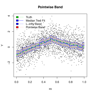
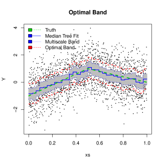
Figure 4: (Left) Pointwise $0.95\%$ credible intervals together with a $95\%$ $L^{\infty}$–credible band (gray area). (Right) Not-intersected multiscale $0.95\%$ credible band (77) (gray area) using $w_{l}=l^{1/2+0.01}$ (see Supplement, Section 7.3.5) together with the ‘optimal’ set (32) obtained with $v_{n}=1$. The true function is $f_{0}(x)=(4x-1)\mathbb{I}(x\leq 1/2)+(-2x+2)\mathbb{I}(x>1/2)$.

3.3 Inference for Functionals of $f_{0}$: Bernstein-von Mises Theorems

By slightly modifying the Bayesian CART prior on the coarsest scales, it is possible to obtain asymptotic normality results, in the form of Bernstein-von Mises theorems, that imply that posterior quantile-credible sets are optimal-size confidence sets. In the next result, $\beta_{S}$ denotes the bounded-Lipschitz metric on the metric space $S$ (see also the Supplement Section 7.3).

Theorem 4.

Assume the Bayesian CART priors $\Pi_{\mathbb{T}}$ from Theorem 1 constrained to trees that fit $j_{0}(n)$ layers, i.e. $\gamma_{lk}=1$ for $l\leq j_{0}(n)$, for $j_{0}(n)\asymp\sqrt{\log{n}}$.

1. BvM for smooth functionals $\psi_{b}(f):={\langle}f,b{\rangle}$. Let $b\in L^{\infty}[0,1]$ with coefficients $(b_{lk}={\langle}b,\psi_{lk}{\rangle})$. Assume $\sum_{k}|b_{lk}|\leq c_{l}$ for all $l\geq 1$ with $\sum_{l}l^{2}c_{l}<\infty$. Then, in $P_{f_{0}}$-probability,

   $$\beta_{\mathbb{R}}\left(\mathcal{L}(\sqrt{n}(\psi_{b}(f)-\hat{\psi}_{b})\,|\,X),\mathcal{L}(\mathcal{N}(0,\|b\|_{2}^{2}))\right)\rightarrow 0.$$

2. Functional BvM for the primitive $F(\cdot)=\int_{0}^{\cdot}f$. Let $(G(t):t\in[0,1])$ be a Brownian motion. Then, in $P_{f_{0}}$-probability,

   $$\beta_{C([0,1])}\left(\mathcal{L}\left(\sqrt{n}(F(\cdot)-\int_{0}^{\cdot}dX^{(n)}\,|\>X)\right),\mathcal{L}(G)\right)\rightarrow 0$$

As a consequence of this result, quantile credible sets for the considered functionals are optimal confidence sets. For $\alpha\in(0,1)$, let $q_{\alpha/2}^{\psi_{b}}(X)$ and $q_{1-\alpha/2}^{\psi_{b}}(X)$ be the $\alpha/2$ and $1-\alpha/2$ quantiles of the induced posterior distribution on the functional $\psi_{b}=\int_{0}^{1}f(u)b(u)du$ and set $I_{b}(X):=[q_{\alpha/2}^{\psi_{b}}(X),q_{1-\alpha/2}^{\psi_{b}}(X)]$. Theorem 4 (part 1) then implies (see [18] for a proof) that

$$P_{f_{0}}\left[\psi_{b}(f_{0})\in I_{b}(X)\right]\to 1-\alpha.$$

Similarly, let $R_{n}(X)$ be the data-dependent radius chosen from the induced posterior distribution on $F(\cdot)=\int_{0}^{\cdot}f$ as follows, for $\hat{F}(\cdot)=\int_{0}^{\cdot}dX^{(n)}$,

$$\Pi[\|F-\hat{F}\|_{\infty}\leq R_{n}(X)\,|\,X]=1-\alpha.$$ (35)

Consider the band $\mathcal{C}^{F}(X):=\{F:\,\|F-\hat{F}\|_{\infty}\leq R_{n}(X)\}$. Then Theorem 4 (part 2) implies (see [18], Corollary 2 for a related statement and proof), for $F_{0}(\cdot)=\int_{0}^{\cdot}f_{0}$,

$$P_{f_{0}}\left[F_{0}\in\mathcal{C}^{F}(X)\right]\to 1-\alpha.$$

In other words, the band (35) has exact asymptotic coverage. It can also be checked that it is optimal efficient in semiparametric terms (that is, its width is optimal asymptotically). We derive Theorem 4 as a consequence of an adaptive nonparametric BvM (Theorem 9 in the Supplement; see Section 10.5 for a proof, where other possible choices for $j_{0}(n)$ are discussed), only obtained so far for adaptive priors in the work of Ray [53], which considered (conjugate) spike and slab priors. Derivation of the band (35) in practice is easily obtained once posterior samples are available. Theorem 4 is illustrated, in the regression framework studied in Section 7.1, on a numerical example with a piece-wise linear regression function (details on the implementation are in Section 7.2) in Figure 5. The left panel presents a histogram of posterior samples (together with $2.5\%$ and $97.5\%$ quantiles) of the rescaled primitive functional $\widetilde{F}(x)=nF(x)=\sum_{t_{i}\leq x}f(t_{i})$ for $x=0.8$ with true value is marked with a red solid line. The right panel portrays the confidence band (35) which uniformly captures the true functional (dotted line).

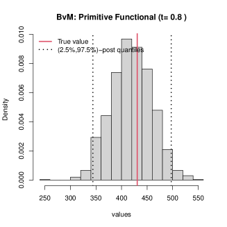
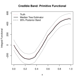
Figure 5: (Left) $0.95\%$ credible interval for the (rescaled) primitive functional $\widetilde{F}(x)$ with $x=0.8$; (Right) the confidence band (35) obtained for $f_{0}(x)=(4x-1)\mathbb{I}(x\leq 1/2)+(-2x+2)\mathbb{I}(x>1/2)$.

3.4 Lower bound: flat trees are (grossly) suboptimal for the $\|\cdot\|_{\infty}$–loss

Recall that the spike-and-slab prior achieves the actual $\ell_{\infty}$–minimax rate without any additional factor. Interestingly, the very same prior misses the $\ell_{2}$–minimax rate by a log factor [43]. This illustrates that $\ell_{2}$ and $\ell_{\infty}$ adaptations require different desiderata when constructing priors. Product priors that correspond to separable rules do not yield adaptation with exact rates in the $\ell_{2}$ sense [12]. Mixture priors that are adaptive in $\ell_{2}$, on the other hand, may not yield $\ell_{\infty}$ adaptation. We now provide one example of this phenomenon in the context of flat (complete binary) trees.

The flat tree of depth $d=d(\mathcal{T})$ is the binary tree which contains all possible nodes until level $d$, i.e. $\gamma_{lk}=\mathbb{I}_{l<d}$. An example of a flat tree with $d=3$ layers is in Figure 2. The simplest possible prior on tree topologies (confined to symmetric trees) is just the Dirac mass at a given flat tree of fixed depth $d=D$; an adaptive version thereof puts a prior $D$ and samples from the set of all flat trees. Such priors coincide with so-called sieve priors, where the sieve spans the expansion basis (e.g. Haar) up to level $D$. Flat dyadic trees only keep Haar wavelet coefficients at resolutions smaller than some $d>0$ (i.e. $\gamma_{lk}=0$ for $l\geq d$). The implied prior on $(\beta_{lk})_{lk}$ can be written as, with $\pi(\beta_{lk})\propto\sigma_{l}^{-1}\phi\left(\beta_{lk}/\sigma_{l}\right)$,

$$(\beta_{lk})\,|\>d \,\sim\,\bigotimes_{l<d,k}\,\pi(\beta_{lk})\ \otimes\ \bigotimes_{l\geq d,k}\,\delta_{0}(\beta_{lk}),$$ (36)

where $\phi(\cdot)$ is some bounded density that is strictly positive on $\mathbb{R}$ and $\sigma_{l}$ are fixed positive scalars. The sequence $(\sigma_{l})$ is customarily chosen so as it decays with the resolution index $l$, e.g. $\sigma_{l}=2^{-l(\beta+1/2)}$ for some $0<\beta\leq\alpha.$ This “undersmoothing” prior requires the knowledge of (a lower bound on) $\alpha$ and yields a non-adaptive non-parametric BvM behavior [18].

A tempting strategy to manufacture adaptation is to treat the threshold $d$ as random through a prior $\pi(d)$ on integers (and take constant $\sigma_{l}$), which corresponds to the hierarchical prior on regular regression histograms [55, 61]. It is not hard to check that the flat-tree prior (36) with random $d$ has a marginal mixture distribution similar to the one of the spike-and-slab prior on each coordinate $(l,k)$. Despite marginally similar, the probabilistic structure of these two priors is very different. Zeroing out signals internally, the spike-and-slab prior (10) is $\ell_{\infty}$–adaptive [43]. The flat tree prior (36), on the other hand, fits a few dense layers without internal sparsity and is $\ell_{2}$–adaptive (up to a log term) [61]. However, as shown in the following Theorem, flat trees fall short of $\ell_{\infty}$–adaptation.

Theorem 5.

Assume the flat tree prior (36) with random $d$, where $\pi(d)$ is non-increasing and where the active wavelet coefficients $\beta_{lk}$ are Gaussian iid $\mathcal{N}(0,1)$. Moreover, assume $\{\psi_{lk}\}$ is an $S$–regular wavelet basis for some $S\geq 1$. For any $0<\alpha\leq S$ and $M>0$, there exists $f_{0}\in\mathcal{H}(\alpha,M)$ such that

$$E_{f_{0}}\Pi\left[\ell_{\infty}(f_{\mathcal{T},\boldsymbol{\beta}},f_{0})<\zeta_{n}\,|\,X\right]\to 0,$$

where the lower-bound rate $\zeta_{n}$ is given by $\zeta_{n}=\left(\frac{\log{n}}{n}\right)^{\frac{\alpha}{2\alpha+2}}.$

Theorem 5, proved in Section 10.6, can be applied to standard priors $\pi(d)$ with exponential decrease, proportional to $\mathrm{e}^{-d}$ or $\mathrm{e}^{-d\log{d}}$, or to a uniform prior over $\{1,\ldots,L_{max}\}$. In [1], a negative result is also derived for sieve-type priors, but only for the posterior mean and for Sobolev classes instead of the, here arguably more natural, Hölder classes for supremum losses (which leads to different rates for estimating the functional–at–a–point). Here, we show that when the target is the $\ell_{\infty}$–loss for Hölder classes the sieve-prior is severely sub-optimal.

3.5 Nonparametric Regression: Overview of Results

Our results obtained under the white noise model can be transported to the more practical nonparametric regression model. While these two models are asymptotically equivalent [10] (under uniform smoothness assumptions satisfied, e.g., by $\alpha$-Hölderian functions with $\alpha>1/2$), it is not automatic that the knowledge of a (wavelet shrinkage/non-linear) minimax procedure in one model implies the optimality in the other. It turns out, however, that our results can be carried over to fixed-design regression without necessarily assuming $\alpha>1/2$. We assume outcomes $Y=(Y_{1},\dots,Y_{n})^{\prime}$ arising from

$$Y_{i}=f_{0}(t_{i})+\varepsilon_{i},\quad\varepsilon_{i}\stackrel{{\scriptstyle iid}}{{\sim}}\mathcal{N}(0,1),\quad i=1,\dots,n=2^{L_{max}+1}$$ (37)

where $f_{0}$ is an unknown regression function and $\{t_{i}\in[0,1]:1\leq i\leq n\}$ are fixed design points. For simplicity, we consider a regular grid, i.e. $t_{i}=i/n$ for $1\leq i\leq n$ and assume $n$ is a power of $2$. In Section 7.1, we show that most results for Bayesian CART obtained earlier in white noise carry over to the model (64) with a few minor changes. One minor modification concerns the loss function. We mainly consider the ‘canonical’ supremum-norm loss for the fixed design setting, that is, the ‘max-norm’ defined for given functions $f,g$ by

$$\|f-g\|_{\infty,n}=\max_{1\leq i\leq n}|f(t_{i})-g(t_{i})|,$$

but it is also possible to consider the whole supremum-norm loss $\|\cdot\|_{\infty}$. We postpone statements and proofs to the Supplement, Sections 7.1 and 12.1. In a numerical study (Section 7.2), we illustrate that the implementation of Bayesian CART [22, 25] and the construction of our confidence bands is rather straightforward. For example, Figure 7 shows how inference can be carried out with Bayesian CART posteriors in non-parametric regression with a piece-wise linear regression function using the intersecting band construction (detailed in Section 7.3.5). Contrary to point-wise credible intervals (on the left) that are easy to produce but do not cover, our multiscale confidence band (on the right) uniformly captures the true regression function. More details on this example are presented in Section 7.2.

4 Non-dyadic Bayesian CART

A limitation of midpoint splits in dyadic trees is that they treat the basis as fixed, allowing the jumps to occur only at pre-specified dyadic locations even when not justified by data. General CART regression methodology [9, 33] avoids this restriction by treating the basis as unknown, where the partitioning cells shrink and stretch with data. In this section, we leave behind ‘static’ dyadic trees to focus on the analysis of Bayesian (non-dyadic) CART [22, 25] and its connection to Unbalanced Haar (UH) wavelet basis selection.

4.1 Unbalanced Haar Wavelets

UH wavelet basis functions [38] are not necessarily translates/dilates of any mother wavelet function and, as such, allow for different support lengths and design-adapted split locations. Here, we particularize the constructive definition of UH wavelets given by [32]. Assume that possible values for splits are chosen from a set of $n=2^{L_{max}}$ breakpoints $\mathcal{X}=\{x_{i}:x_{i}=i/n,1\leq i\leq n\}$. Using the scale/location index enumeration, pairs $(l,k)$ in the tree are now equipped with (a) a breakpoint $b_{lk}\in\mathcal{X}$ and (b) left and right brackets $(l_{lk},r_{lk})\in\mathcal{X}\cup\{0,1\}$. Unlike balanced Haar wavelets (3), where $b_{lk}=(2k+1)/2^{l+1}$, the breakpoints $b_{lk}$ are not required to be regularly dyadically constrained and are chosen from $\mathcal{X}$ in a hierarchical fashion as follows. One starts by setting $l_{00}=0,r_{00}=1$. Then

• The first breakpoint $b_{00}$ is selected from $\mathcal{X}\cap(0,1)$.

• For each $1\leq l\leq L_{max}$ and $0\leq k<2^{l}$, set

  $$l_{lk}=l_{(l-1)\lfloor k/2\rfloor},\quad \quad r_{lk}=b_{(l-1)\lfloor k/2\rfloor},\quad\text{if $k$ is even},$$ (38)

  $$l_{lk}=b_{(l-1)\lfloor k/2\rfloor},\quad \quad r_{lk}=r_{(l-1)\lfloor k/2\rfloor},\quad\text{if $k$ is odd}.$$

  If $\mathcal{X}\cap(l_{lk},r_{lk}]\neq\emptyset,$ choose $b_{lk}$ from $\mathcal{X}\cap(l_{lk},r_{lk}]$.

Let $A$ denote the set of admissible nodes $(l,k)$, in that $(l,k)$ is such that $\mathcal{X}\cap(l_{lk},r_{lk}]\neq\emptyset$, obtained through an instance of the sampling process described above and let

$$B=(b_{lk})_{(l,k)\in A}$$

be the corresponding set of breakpoints. Each collection of split locations $B$ gives rise to nested intervals

$$L_{lk}=(l_{lk},b_{lk}]\,\quad\text{and}\quad R_{lk}=(b_{lk},r_{lk}].$$

Starting with the mother wavelet $\psi_{-10}^{B}=\psi_{-10}=\mathbb{I}_{(0,1)}$, one then recursively constructs wavelet functions $\psi_{lk}^{B}$ with a support $I_{lk}^{B}=L_{lk}\cup R_{lk}$ as

$$\psi_{lk}^{B}(x)=\frac{1}{\sqrt{|L_{lk}|^{-1}+|R_{lk}|^{-1}}}\left(\frac{\mathbb{I}_{L_{lk}}(x)}{|L_{lk}|}-\frac{\mathbb{I}_{R_{lk}}(x)}{|R_{lk}|}\right).$$ (39)

By construction, the system $\Psi_{A}^{B}=\{\psi_{-10}^{B},\psi_{lk}^{B}:(l,k)\in A\}$ is orthonormal in $L^{2}[0,1]$. With UH wavelets, the decay of wavelet coefficients $\beta_{lk}={\langle}f,\psi_{lk}^{B}{\rangle}$ for a $\alpha$–Hölder function $f$ verifies $|\beta_{lk}^{B}|\lesssim\max\{|L_{lk}|,|R_{lk}|\}^{\alpha+1/2}$, see Lemma 9. [32] points out that the computational complexity of the discrete UH transform could be unnecessarily large and imposes the balancing requirement $\max\left\{|L_{lk}|,|R_{lk}|\right\}\leq E(|L_{lk}|+|R_{lk}|)\ \forall(l,k)\in A$, for some $1/2\leq E<1$. Similarly, in order to control the combinatorial complexity of the basis system, we require that the UH wavelets are weakly balanced in the following sense.

Definition 5.

A system $\Psi_{A}^{B}=\{\psi_{-10}^{B},\psi_{lk}^{B}:(l,k)\in A\}$ of UH wavelets is weakly balanced with balancing constants $E,D\in\mathbb{N}^{*}$ if, for any $(l,k)\in A$,

$$\max\limits\left(|L_{lk}|,|R_{lk}|\right)=\frac{M_{lk}}{2^{l+D}}\quad\text{for some $M_{lk}\in\{1,\dots,E+l\}$}.$$ (40)

Note that in the actual BART implementation, the splits are chosen from sample quantiles to ensure balancedness (similar to our condition (40)). Quantile splits (Example 2 below) are a natural way to generate many weakly balanced systems, providing a much increased flexibility compared to dyadic splits, which correspond to uniform quantiles. Other examples together with a graphical depiction of the unbalanced Haar wavelets for certain non-dyadic choices of split points $b_{lk}$ are in the Supplement (Figure 9 in Section 9).

Example 2 (Quantile Splits).

Denote with $G$ a c.d.f with a density $g$ on $[0,1]$ that satisfies $\|g\|_{\infty}\leq 2^{D-1}/(2E)$ for $E,D>0$ chosen below and $\|1/g\|_{\infty}\leq C_{q}$ for some $C_{q}>0$. Let us define a dyadic projection of $G$ as

$$G_{l}^{-1}(x):=2^{-l}\lfloor 2^{l}G^{-1}(x)\rfloor,$$

and next define the breakpoints, for ${l\leq L_{max}}$ and $0\leq k<2^{l}$, as

$$b_{lk}=G_{L_{max}+D}^{-1}[(2k+1)/2^{l+1}].$$ (41)

The system $\Psi_{A}^{B}$ obtained from steps (a) and (b) with splits (41) is weakly balanced for $E=2+3C_{q}2^{D-1}$. This is verified in Lemma 12 in the Appendix (Section 9.4). Moreover, Figure 6(a) in illustrates the implementation of the quantile system, where splits are placed more densely in areas where $G(x)$ changes more rapidly.

(a) $g(x)\sim\mathcal{B}(1,1)$

(b) $g(x)\sim\mathcal{B}(2,5)$

Figure 6: Example of quantile splits for a uniform density $g(x)$ and a non-uniform beta density $g(x)$ using $L_{max}=6$.

The non-dyadic Bayesian CART prior is then defined as follows:

• Step 1. (Basis Generation) Sample $B=(b_{lk})_{0\leq k<2^{l}-1,l\leq L}$ from $\Pi_{\mathbb{B}}$ by following the steps a)–b) around (38) subject to satisfying the balancing condition (40).

• Step 2. (Tree Generation) Independently of $B$, sample a binary tree $\mathcal{T}$ from one of the priors $\Pi_{\mathbb{T}}$ described in Section 2.1.

• Step 3. (Step Heights Generation) Given $\mathcal{T}$, we obtain the coefficients $(\beta_{lk}^{B})$ from the tree-shaped prior (19). Using the UH wavelets, the prior on the internal coefficients $\beta_{lk}^{B}$ can be translated into a model on the histogram heights $\widetilde{\beta}_{lk}^{B}$ through (8).

An example of such a prior is obtained by first randomly drawing quantiles (e.g. by drawing a density at random verifying conditions as in Example 2) to generate the breakpoints for Step 1 and then following the construction from Section 2 for Steps 2–3. The following theorem is proved in Section 11.

Theorem 6.

Let $\Pi_{\mathbb{B}}$ be any prior on breakpoint collections that satisfy weak balancedness according to Definition 5. Let $\Pi_{\mathbb{T}}$ be the Galton-Watson process prior from Section 2.1 with $p_{lk}=\Gamma^{-l^{4}}$. Consider the tree-shaped wavelet prior (19) with $\pi(\boldsymbol{\beta}_{\mathcal{T}})\sim\mathcal{N}(0,I_{|\mathcal{T}_{ext}|})$. Let $f_{0}\in\mathcal{H}^{\alpha}_{M}$ as in (24) for some $M>0$ and $0<\alpha\leq 1$ and define

$$\varepsilon_{n}=(\log{n})^{1+\frac{3}{2}}\left(\frac{\log{n}}{n}\right)^{\frac{\alpha}{2\alpha+1}}.$$ (42)

Then, there exist $\Gamma_{0},c_{0}>0$ depending only on the constants $E,D$ in the weak balancedness condition such that, for any $\Gamma\geq\Gamma_{0}$ and $c\geq c_{0}$, for any $M_{n}\to\infty$, we have, for $n\rightarrow\infty$

$$E_{f_{0}}\Pi\left[\,\ell_{\infty}(f_{\mathcal{T},\boldsymbol{\beta}},f_{0})\geq\|f_{\mathcal{T},\boldsymbol{\beta}}-f_{0}\|_{\infty}>M_{n}\varepsilon_{n}\,|\,X\right]\to 0.$$ (43)

In the context of piecewise constant priors, Theorem 6 allows further flexibility in the choice of the prior as compared to Theorem 1 in that the location of the breakpoints, on the top of their structure given by the tree prior, can vary in their location according to its own specific prior. Whether one can further weaken the balancing condition to still get optimal multiscale results is an interesting open question that goes beyond the scope of this paper. In addition, the log-factor in (42) could be further optimized, similarly as in Theorem 1.

5 Discussion

In this paper we explored connections between Bayesian tree-based regression methods and structured wavelet shrinkage. We demonstrated that Bayesian tree-based methods attain (almost) optimal convergence rates in the supremum norm and obtain limiting results for functionals, that follow from a non-parametric and adaptive Bernstein–von Mises theorem. The developed framework also allows us to construct adaptive credible bands around $f_{0}$ under self-similarity. To allow for non-dyadically organized splits, we introduced weakly balanced Haar wavelets (an elaboration on unbalanced Haar wavelets of [38]) and showed that Bayesian CART performs basis selection from this library and attains a near-minimax rate of posterior concentration under the sup-norm loss.

Although for clarity of exposition we focused on the white noise model, our results can be extended to the more practical regression model for fixed regular designs (Section 7.1 in the Supplement) or possibly more general designs under some conditions. We note that the techniques of proof are non-conjugate in their key tree aspect, which opens the door to applications in many other statistical settings. A version of Bayesian CART for density estimation following the ideas of the present work is currently investigated by T. Randrianarisoa as part of his PhD thesis. More precisely, using the present techniques, it is possible to develop multiscale rate results for Pólya trees with ‘optional stopping’ along a tree, in the spirit of [66]. Our confidence set construction can be also shown to have local adaptation properties. The ability of Bayesian CART to spatially adapt in this way will be investigated in a followup work. Further natural extensions include high-dimensional versions of the model, extending the multi-dimensional version briefly presented here, as well as forest priors. These will be considered elsewhere.

6 Proof of Theorem 1

The proof proceeds in three steps. In Section 6.1 we first show that the posterior concentrates on not too deep trees. In Section 6.2, we then show that the posterior probability of missing signal vanishes and, finally, in Section 6.3 we show that the posterior distribution concentrates around signals. To better convey main ideas, we present the proof for the independent prior $\boldsymbol{\beta}_{\mathcal{T}}\sim\mathcal{N}(0,\Sigma_{\mathcal{T}})$ with $\Sigma_{\mathcal{T}}=I_{K}$ for $K=|\mathcal{T}_{ext}|$ and the Galton-Watson (GW) tree prior from Section 2.1.1 with a split probability $p_{l}$. The proof for the $g$-prior $\Sigma_{\mathcal{T}}=g_{n}(A_{\mathcal{T}}^{\prime}A_{\mathcal{T}})^{-1}$ is more technically involved and is presented in Section 10.1 in the Supplement.

We will be working conditionally on the event

$$\mathcal{A}=\left\{\max_{-1\leq l\leq L,\,0\leq k<2^{l}}\varepsilon_{lk}^{2}\leq 2\log\left(2^{L+1}\right)\right\},$$ (44)

where $L=L_{max}=\lfloor\log_{2}n\rfloor$. Since $\varepsilon_{lk}\sim\mathcal{N}(0,1)$, this event has a large probability in the sense that $P(\mathcal{A}^{c})\lesssim(\log n)^{-1}$, which follows from $P\left[\max\limits_{1\leq i\leq N}|Z_{i}|>\sqrt{2\log N}\right]\leq c_{0}/\sqrt{\log N}$ for some $c_{0}>0$ when $Z_{i}\sim\mathcal{N}(0,1)$ for $1\leq i\leq N$.

6.1 Posterior Probability of Deep Trees

The first step is to show that, on the event $\mathcal{A}$, the posterior concentrates on reasonably small trees, i.e. trees whose depth $d(\mathcal{T})$ is no larger than an ‘optimal’ depth which depends on the unknown smoothness $\alpha$. Let us define such a depth $\mathcal{L}_{c}=\mathcal{L}_{c}(\alpha,M)$ as

$${\mathcal{L}_{c}}=\left\lceil\log_{2}\left((8M)^{\frac{1}{\alpha+1/2}}\left(\frac{n}{\log{n}}\right)^{\frac{1}{2\alpha+1}}\right)\right\rceil.$$ (45)

Lemma 1.

Under the assumptions of Theorem 1, on the event $\mathcal{A}$,

$$\Pi[d(\mathcal{T})>\mathcal{L}_{c}\,|\>X]\rightarrow 0\quad(n\rightarrow\infty).$$ (46)

Proof.

Consider one tree $\mathcal{T}\in\mathbb{T}$ such that $d(\mathcal{T})\geq 1$ and denote with $\mathcal{T}^{-}$ a pruned subtree obtained from $\mathcal{T}$ by turning its deepest rightmost internal node, say $(l_{1},k_{1})$, into a terminal node. Then $\mathcal{T}^{-}=\mathcal{T}_{int}^{-}\cup\mathcal{T}_{ext}^{-}$, where

$$\mathcal{T}_{int}^{-}=\mathcal{T}_{int}\backslash\{(l_{1},k_{1})\},\quad\mathcal{T}_{ext}^{-}=\mathcal{T}_{ext}\backslash\{(l_{1}+1,2k_{1}),(l_{1}+1,2k_{1}+1)\}\cup\{(l_{1},k_{1})\}.$$

Note that $\mathcal{T}^{-}$ is a full binary tree and that the mapping $\mathcal{T}\rightarrow\mathcal{T}^{-}$ is not necessarily injective. Indeed, there are up to $2^{d(\mathcal{T}^{-})}$ trees $\mathcal{T}$ that give rise to the same pruned tree $\mathcal{T}^{-}$. Let $\mathbb{T}_{d}=\{\mathcal{T}\in\mathbb{T}:d(\mathcal{T})=d\}$ denote the set of all full binary trees of depth exactly $d\geq 1$. Then, using the notation (22),

$$\Pi[\mathbb{T}_{d}\,|\,X] =\frac{\sum_{\mathcal{T}\in\mathbb{T}_{d}}W_{X}(\mathcal{T})}{\sum_{\mathcal{T}\in\mathbb{T}}W_{X}(\mathcal{T})}=\frac{\sum_{\mathcal{T}\in\mathbb{T}_{d}}\frac{W_{X}(\mathcal{T})}{W_{X}(\mathcal{T}^{-})}W_{X}(\mathcal{T}^{-})}{\sum_{\mathcal{T}\in\mathbb{T}}W_{X}(\mathcal{T})},$$ (47)

$$\text{where}\qquad\frac{W_{X}(\mathcal{T})}{W_{X}(\mathcal{T}^{-})}=\frac{\Pi_{\mathbb{T}}(\mathcal{T})}{\Pi_{\mathbb{T}}(\mathcal{T}^{-})}\frac{\int\prod_{(l,k)\in\mathcal{T}_{int}^{\prime}}\mathrm{e}^{nX_{lk}\beta_{lk}-n\beta_{lk}^{2}/2}d\pi(\boldsymbol{\beta}_{\mathcal{T}})}{\int\prod_{(l,k)\in{\mathcal{T}_{int}^{-}}^{\prime}}\mathrm{e}^{nX_{lk}\beta_{lk}-n\beta_{lk}^{2}/2}d\pi(\boldsymbol{\beta}_{\mathcal{T}^{-}})}.$$

Let $\boldsymbol{X}_{\mathcal{T}}=(X_{lk}:(l,k)\in\mathcal{T}_{int}^{\prime})^{\prime}$ and $\boldsymbol{\beta}_{\mathcal{T}}=(\beta_{lk}:(l,k)\in\mathcal{T}_{int}^{\prime})^{\prime}$ be the top-down left-to-right ordered sequences (recall that we order nodes according to the index $2^{l}+k$). Assuming $\boldsymbol{\beta}_{\mathcal{T}}\sim\mathcal{N}(0,\Sigma_{\mathcal{T}})$, and denoting $K=|\mathcal{T}_{ext}|=|\mathcal{T}_{int}|+1$,

$$\frac{W_{X}(\mathcal{T})}{W_{X}(\mathcal{T}^{-})} =\frac{\Pi_{\mathbb{T}}(\mathcal{T})}{\Pi_{\mathbb{T}}(\mathcal{T}^{-})}\sqrt{\frac{{|\Sigma_{\mathcal{T}^{-}}|}}{2\pi{|\Sigma_{\mathcal{T}}|}}}\frac{\int\mathrm{e}^{n\boldsymbol{X}_{\mathcal{T}}^{\prime}\boldsymbol{\beta}_{\mathcal{T}}-\boldsymbol{\beta}_{\mathcal{T}}^{\prime}[nI_{K}+\Sigma_{\mathcal{T}}^{-1}]\boldsymbol{\beta}_{\mathcal{T}}/2}d\boldsymbol{\beta}_{\mathcal{T}}}{\int\mathrm{e}^{n\boldsymbol{X}_{\mathcal{T}^{-}}^{\prime}\boldsymbol{\beta}_{\mathcal{T}^{-}}-\boldsymbol{\beta}_{\mathcal{T}^{-}}^{\prime}[nI_{K-1}+\Sigma_{\mathcal{T}^{-}}^{-1}]\boldsymbol{\beta}_{\mathcal{T}^{-}}/2}d\boldsymbol{\beta}_{\mathcal{T}^{-}}}$$

$$=\frac{\Pi_{\mathbb{T}}(\mathcal{T})}{\Pi_{\mathbb{T}}(\mathcal{T}^{-})}\sqrt{\frac{{|\Sigma_{\mathcal{T}^{-}}|}}{{|\Sigma_{\mathcal{T}}|}}}\sqrt{\frac{{|nI_{K-1}+\Sigma_{\mathcal{T}^{-}}^{-1}|}}{{|nI_{K}+\Sigma_{\mathcal{T}}^{-1}|}}}\frac{\mathrm{e}^{n^{2}\boldsymbol{X}_{\mathcal{T}}^{\prime}(nI_{K}+\Sigma_{\mathcal{T}}^{-1})^{-1}\boldsymbol{X}_{\mathcal{T}}/2}}{\mathrm{e}^{n^{2}\boldsymbol{X}_{\mathcal{T}^{-}}^{\prime}(nI_{K-1}+\Sigma_{\mathcal{T}^{-}}^{-1})^{-1}\boldsymbol{X}_{\mathcal{T}^{-}}/2}}.$$ (48)

Since $X_{l_{1}k_{1}}$ corresponds to the node $(l,k)$ with the highest index $2^{l}+k$, one can write $\boldsymbol{X}_{\mathcal{T}}=(\boldsymbol{X}_{\mathcal{T}^{-}},X_{l_{1}k_{1}})^{\prime}$.

We focus on the GW prior from Section 2.1.1 and on the independent prior $\Sigma_{\mathcal{T}}=I_{K}$ and present proofs for the remaining priors in Section 10.1. Using the expression (48) and since $(l_{1},k_{1})$ is the deepest rightmost internal node in $\mathcal{T}$, and $\mathcal{T}$ is of depth $d=d(\mathcal{T})=l_{1}+1$, using the definition of the GW prior,

$$\frac{W_{X}(\mathcal{T})}{W_{X}(\mathcal{T}^{-})}=\frac{\Pi_{\mathbb{T}}(\mathcal{T})}{\Pi_{\mathbb{T}}(\mathcal{T}^{-})}\prod_{(l,k)\in\mathcal{T}_{int}^{\prime}\setminus\mathcal{T}_{int}^{\prime-}}\frac{\mathrm{e}^{\frac{n^{2}}{2(n+1)}X_{lk}^{2}}}{\sqrt{n+1}}=\frac{p_{d-1}(1-p_{d})^{2}}{1-p_{d-1}}\frac{\mathrm{e}^{\frac{n^{2}}{2(n+1)}X_{l_{1}k_{1}}^{2}}}{\sqrt{n+1}}.$$

Suppose $\mathcal{T}$ has depth $d(\mathcal{T})>\mathcal{L}_{c}$. Then $l_{1}\geq\mathcal{L}_{c}$ and from the Hölder continuity (23), one gets $8|\beta_{l_{1}k_{1}}|\leq\sqrt{\log{n}/n}$, where $\mathcal{L}_{c}$ is as in (45). Then, conditionally on the event (44),

$$|X_{l_{1}k_{1}}|\leq\frac{1}{\sqrt{n}}\left[\frac{1}{8}\sqrt{\log{n}}+\sqrt{2\log{n}+\log{4}}\right]$$ (49)

and thereby $2X_{l_{1}k_{1}}^{2}\leq 5\log{n}/n$. Recall that, under the GW-prior, the split probability is $p_{d}=\Gamma^{-d}$. As $\Gamma>2$, one has $p_{d}<1/2$ and so, for any $d>\mathcal{L}_{c}$,

$$\frac{W_{X}(\mathcal{T})}{W_{X}(\mathcal{T}^{-})}\leq 2\,p_{d-1}\exp\left(\frac{5\,n\log n}{4(n+1)}-\frac{1}{2}\log(1+n)\right)<2n^{3/4}p_{d-1}.$$

Going back to the ratio (47), we now bound, with $a(n,d)\eqqcolon 2n^{3/4}p_{d-1}$,

$$\frac{\Pi[\mathbb{T}_{d}\,|\,X]}{a(n,d)}\leq\frac{\sum_{\mathcal{T}\in\mathbb{T}_{d}}W_{X}(\mathcal{T}^{-})}{\sum_{\mathcal{T}\in\mathbb{T}}W_{X}(\mathcal{T})}\leq\frac{\sum_{\mathcal{T}\in\mathbb{T}_{d}^{-}}2^{d(\mathcal{T}^{-})}W_{X}(\mathcal{T})}{\sum_{\mathcal{T}\in\mathbb{T}}W_{X}(\mathcal{T})}\leq 2^{d},$$

where $\mathbb{T}_{d}^{-}$ is the image of $\mathbb{T}_{d}$ under the map $\mathcal{T}\to\mathcal{T}^{-}$, and using that at most $2^{d(\mathcal{T}^{-})}$ trees are mapped to the same $\mathcal{T}^{-}$. Using this bound one deduces that, on the event $\mathcal{A}$, with $L=L_{max}=\log_{2}{n}$,

$$\Pi[d(\mathcal{T})>\mathcal{L}_{c}\,|\,X] =\sum_{d=\mathcal{L}_{c}+1}^{L}\Pi[\mathbb{T}_{d}\,|\,X]\leq 4\,n^{3/4}\sum_{d=\mathcal{L}_{c}+1}^{L}2^{d-1}p_{d-1}$$

$$<4\,n^{3/4}\,L\exp\left[-\mathcal{L}_{c}\log(\Gamma/2)\right].$$

As $\mathcal{L}_{c}\asymp(\log{n})/(1+2\alpha),$ the right hand side goes to zero as soon as, e.g. $\log(\Gamma/2)>7(1+2\alpha)/8$ that is, for $\alpha\leq 1$, $\Gamma>2e^{3}$. ∎

6.2 Posterior Probability of Missing Signal

The next step is showing that the posterior probability of missing a node with large enough signal vanishes.

Lemma 2.

Let us denote, for $A>0$ to be chosen suitably large,

$$S(f_{0};A)=\left\{(l,k):\ |\beta_{lk}^{0}|\geq A\frac{\log{n}}{\sqrt{n}}\right\}.$$ (50)

Under the assumptions of Theorem 1, on the event $\mathcal{A}$ from (44),

$${\Pi\left[\left\{\mathcal{T}:\,S(f_{0};A)\nsubseteq\mathcal{T}\right\}\,|\>X\right]\rightarrow 0\qquad(n\to\infty).}$$ (51)

Proof.

As before, we present the proof with the GW prior from Section 2.1.1 and for the independent prior with $\Sigma_{\mathcal{T}}=I_{K}$, referring to Section 10.1 for the $g$-prior. Let us first consider a given node $(l_{S},k_{S})\in S(f_{0};A)$, for $A$ to be specified below, and note that the Hölder condition on $f_{0}$ implies $l_{S}\leq\mathcal{L}_{c}$ (for $n$ large enough). Let $\mathbb{T}_{\setminus(l_{S},k_{S})}=\{\mathcal{T}\in\mathbb{T}:(l_{S},k_{S})\notin\mathcal{T}_{int}\}$ denote the set of trees that miss the signal node in the sense that they do not have a cut at $(l_{S},k_{S})$. For any such tree $\mathcal{T}\in\mathbb{T}_{\setminus(l_{S},k_{S})}$ we then denote by $\mathcal{T}^{+}$ the smallest full binary tree (in terms of the number of nodes) that contains $\mathcal{T}$ and that splits on $(l_{S},k_{S})$. Such a tree can be constructed from $\mathcal{T}\in\mathbb{T}_{\setminus(l_{S},k_{S})}$ as follows. Denote by $(l_{0},k_{0})\in\mathcal{T}_{ext}\cap[(0,0)\leftrightarrow(l_{S},k_{S})]$ the external node of $\mathcal{T}$ which is closest to $(l_{S},k_{S})$ on the route from the root to $(l_{S},k_{S})$ in a flat tree (denoted by $[(0,0)\leftrightarrow(l_{S},k_{S})]$). Next, denote by $\mathcal{T}^{+}$ the extended tree obtained from $\mathcal{T}$ by sequentially splitting all $(l,k)\in[(l_{0},k_{0})\leftrightarrow(l_{S},k_{S})]$. Similarly as for $\mathcal{T}\to\mathcal{T}^{-}$ above, the map $\mathcal{T}\rightarrow\mathcal{T}^{+}$ is not injective and we denote by $\mathbb{T}_{(l_{S},k_{S})}$ the set of all extended trees $\mathcal{T}^{+}$ obtained from some $\mathcal{T}\in\mathbb{T}_{\backslash(l_{S},k_{S})}$. Now, the posterior probability $\Pi\left[\mathbb{T}_{\setminus(l_{S},k_{S})}\,|\,X\right]$ of missing the signal node $(l_{S},k_{S})$ equals

$$\frac{\sum_{\mathcal{T}\in\mathbb{T}_{\setminus(l_{S},k_{S})}}W_{X}(\mathcal{T})}{\sum_{\mathcal{T}\in\mathbb{T}}W_{X}(\mathcal{T})}\leq\frac{\sum_{\mathcal{T}\in\mathbb{T}_{\setminus(l_{S},k_{S})}}\frac{W_{X}(\mathcal{T})}{W_{X}(\mathcal{T}^{+})}W_{X}(\mathcal{T}^{+})}{\sum_{\mathcal{T}\in\mathbb{T}_{(l_{S},k_{S})}}W_{X}(\mathcal{T})}.$$ (52)

Let us denote by $\mathcal{T}^{(j)}$ for $j=-1,\dots,s$ the sequence of nested trees obtained by extending one branch of $\mathcal{T}$ towards $(l_{S},k_{S})$ by splitting the nodes $[(l_{0},k_{0})\leftrightarrow(l_{S},k_{S})]$, where $\mathcal{T}^{+}=\mathcal{T}^{(s)}$ and $\mathcal{T}=\mathcal{T}^{(-1)}$. Then

$$\frac{W_{X}(\mathcal{T})}{W_{X}(\mathcal{T}^{+})}=\frac{\Pi_{\mathbb{T}}(\mathcal{T})}{\Pi_{\mathbb{T}}(\mathcal{T}^{+})}\prod_{j=0}^{s}\frac{N_{X}(\mathcal{T}^{(j-1)})}{N_{X}(\mathcal{T}^{(j)})}.$$ (53)

Under the GW process prior with $p_{l}=\Gamma^{-l}$ for some $\Gamma>2$, the ratio of prior tree probabilities in the last expression satisfies

$$\frac{\Pi_{\mathbb{T}}(\mathcal{T})}{\Pi_{\mathbb{T}}(\mathcal{T}^{+})}=\frac{1-p_{l_{0}}}{p_{l_{0}}}\times\left(\prod_{l=l_{0}+1}^{l_{S}}\frac{1}{p_{l}(1-p_{l})}\right)\times\frac{1}{(1-p_{l_{S}+1})^{2}}.$$ (54)

The first term is due to the fact that $\mathcal{T}^{+}$ splits the node $(l_{0},k_{0})$ while $\mathcal{T}$ does not. The second term in the denominator is the extra prior probability of $\mathcal{T}^{+}$ over $\mathcal{T}$ that is due to the branch reaching out to $(l_{S},k_{S})$. Along this branch (note that this is the smallest possible branch), one splits only one daughter node for each layer $l$ (thereby the term $p_{l}$) and not the other (thereby the term $1-p_{l}$). The third term above is due to the fact that the two daughters of $(l_{S},k_{S})$ are not split. The quantity (54) is bounded by $2^{l_{S}-l_{0}+2}\Gamma^{(l_{0}+l_{S})(l_{S}-l_{0}+1)/2}<4\Gamma^{2l_{S}^{2}}$.

Assuming $\Sigma_{\mathcal{T}}=I_{K}$, we can write for any $\mathcal{T}$ in $\mathbb{T}_{\setminus(l_{S},k_{S})}$

$$\frac{W_{X}(\mathcal{T})}{W_{X}(\mathcal{T}^{+})}=\frac{\Pi_{\mathbb{T}}(\mathcal{T})}{\Pi_{\mathbb{T}}(\mathcal{T}^{+})}\prod_{(l,k)\in\mathcal{T}^{+}\setminus\mathcal{T}}\frac{\sqrt{n+1}}{\mathrm{e}^{\frac{n^{2}}{2(n+1)}X_{lk}^{2}}}.$$ (55)

Using the definition of the model and the inequality $2ab\geq-a^{2}/2-2b^{2}$ for $a,b\in\mathbb{R}$, we obtain $X_{l_{S}k_{S}}^{2}\geq(\beta_{l_{S}k_{S}}^{0})^{2}/2-\varepsilon_{l_{S}k_{S}}^{2}/n$. On the event $\mathcal{A}$, one gets

$$\exp\left\{-\frac{n^{2}}{2(n+1)}X_{l_{S}k_{S}}^{2}\right\}\leq\exp\left\{-\frac{n^{2}(\beta_{l_{S}k_{S}}^{0})^{2}}{4(n+1)}+\frac{n(\log 2)(\log_{2}n+1)}{n+1}\right\}.$$

The term in (55) can be thus bounded, for any $\mathcal{T}\in\mathbb{T}_{\setminus(l_{S},k_{S})}$, by

$$\frac{W_{X}(\mathcal{T})}{W_{X}(\mathcal{T}^{+})}\leq C\Gamma^{2l_{S}^{2}}\,\exp\left\{\frac{3(l_{S}-l_{0}+1)(\log_{2}n+1)}{2}-\frac{nA^{2}\log^{2}{n}}{4(n+1)}\right\}\eqqcolon b(n,l_{S}).$$

We now continue to bound the ratio (52). For each given $\mathcal{T}^{+}$, there are at most $l_{S}$ trees $\widetilde{\mathcal{T}}\in\mathbb{T}_{\backslash(l_{S},k_{S})}$ which have the same extended tree $\widetilde{\mathcal{T}}^{+}=\mathcal{T}^{+}$. This is because $\mathcal{T}^{+}$ is obtained by extending one given branch by adding no more than $l_{S}$ nodes. Using this fact, (52), and the definition of $b(n,l_{S})$ on the last display,

$$\frac{\Pi\left[\mathbb{T}_{\setminus(l_{S},k_{S})}\,|\,X\right]}{b(n,l_{S})}\leq\frac{\sum_{\mathcal{T}\in\mathbb{T}_{\setminus(l_{S},k_{S})}}W_{X}(\mathcal{T}^{+})}{\sum_{\mathcal{T}\in\mathbb{T}_{(l_{S},k_{S})}}W_{X}(\mathcal{T})}\leq\,l_{S}\frac{\sum_{\mathcal{T}\in\mathbb{T}_{(l_{S},k_{S})}}W_{X}(\mathcal{T})}{\sum_{\mathcal{T}\in\mathbb{T}_{(l_{S},k_{S})}}W_{X}(\mathcal{T})}.$$

By choosing $A=A(\Gamma)>0$ large enough, this leads to

$$\Pi\left[\mathbb{T}_{\setminus(l_{S},k_{S})}\,|\>X\right]\lesssim\mathrm{e}^{(3/2+3\log\Gamma)(\log_{2}n+1)^{2}-\frac{A^{2}}{8}\log^{2}{n}}\lesssim\mathrm{e}^{-\frac{A^{2}}{16}\log^{2}n}.$$

Then the result follows as, on the event $\mathcal{A}$,

$$\sum_{(l_{S},k_{S})\in S(f_{0},A)}\Pi\left[\mathbb{T}_{\setminus(l_{S},k_{S})}\,|\,X\right]\lesssim 2^{\mathcal{L}_{c}+1}\mathrm{e}^{-\frac{A^{2}}{16}\log^{2}{n}}\lesssim\mathrm{e}^{-\frac{A^{2}}{32}\log^{2}{n}}\rightarrow 0.\qed$$

6.3 Posterior Concentration Around Signals

Let us now show that the posterior does not distort large signals too much.

Lemma 3.

Let us denote, for $\mathcal{L}_{c}$ as in (45) and $S(f_{0};A)$ as in (50),

$$\mathsf{T}=\{\mathcal{T}:d(\mathcal{T})\leq\mathcal{L}_{c},\ S(f_{0};A)\subset\mathcal{T}\}.$$ (56)

Then, on the event $\mathcal{A}$, for some $C^{\prime}>0$, uniformly over $\mathcal{T}\in\mathsf{T}$,

$$\int\max_{(l,k)\in\mathcal{T}_{int}^{\prime}}|\beta_{lk}-\beta_{lk}^{0}|d\Pi[\boldsymbol{\beta}_{\mathcal{T}}\,|\,\boldsymbol{X}_{\mathcal{T}}]<C^{\prime}\sqrt{\frac{\log n}{n}},$$ (57)

with $\boldsymbol{X}_{\mathcal{T}}=(X_{lk}:(l,k)\in\mathcal{T}_{int}^{\prime})^{\prime}$ the ordered vector of active responses.

Proof.

For a given tree $\mathcal{T}$ with $K=|\mathcal{T}_{ext}|$ leaves, we denote by $\boldsymbol{\beta}_{\mathcal{T}}=(\beta_{lk}:(l,k)\in\mathcal{T}_{int}^{\prime})^{\prime}$ the vector of wavelet (internal node) coefficients, with $\boldsymbol{X}_{\mathcal{T}}$ the corresponding responses and with $\boldsymbol{\varepsilon}_{\mathcal{T}}$ the white noise disturbances. It follows from (21) that, given $\boldsymbol{X}_{\mathcal{T}}$ (so for fixed $\varepsilon_{lk}$) and $\mathcal{T}$, the vector $\boldsymbol{\beta}_{\mathcal{T}}$ has a Gaussian distribution $\boldsymbol{\beta}_{\mathcal{T}}\,|\>\boldsymbol{X}_{\mathcal{T}}\sim\mathcal{N}(\boldsymbol{\mu}_{\mathcal{T}},\widetilde{\Sigma}_{\mathcal{T}}),$ where $\widetilde{\Sigma}_{\mathcal{T}}=(nI_{K}+\Sigma_{\mathcal{T}}^{-1})^{-1}$ and $\boldsymbol{\mu}_{\mathcal{T}}=n\widetilde{\Sigma}_{\mathcal{T}}\left(\boldsymbol{\beta}^{0}_{\mathcal{T}}+\frac{1}{\sqrt{n}}\boldsymbol{\varepsilon}_{\mathcal{T}}\right).$ Next, using Lemma 7, we have

$$\mathbb{E\,}\left[\|\boldsymbol{\beta}_{\mathcal{T}}-\boldsymbol{\beta}^{0}_{\mathcal{T}}\|_{\infty}\,|\,\boldsymbol{X}_{\mathcal{T}}\right] \leq\|\boldsymbol{\mu}_{\mathcal{T}}-\boldsymbol{\beta}^{0}_{\mathcal{T}}\|_{\infty}+\sqrt{2\,\bar{\sigma}^{2}\log K}+2\sqrt{2\pi\bar{\sigma}^{2}},$$ (58)

where $\bar{\sigma}^{2}=\max\mathrm{diag}(\widetilde{\Sigma}_{\mathcal{T}})$. Focusing on the first term, we can write

$$\|\boldsymbol{\mu}_{\mathcal{T}}-\boldsymbol{\beta}^{0}_{\mathcal{T}}\|_{\infty} \leq\sqrt{n}\|\widetilde{\Sigma}_{\mathcal{T}}\boldsymbol{\varepsilon}_{\mathcal{T}}\|_{\infty}+\|(n\widetilde{\Sigma}_{\mathcal{T}}-I_{K})\boldsymbol{\beta}_{\mathcal{T}}^{0}\|_{\infty}.$$ (59)

Using the fact $(I+B)^{-1}=I-(I+B^{-1})^{-1}$, we obtain $n\widetilde{\Sigma}_{\mathcal{T}}-I_{K}=-(I_{K}+n\Sigma_{\mathcal{T}})^{-1}$. From now on, we focus on the simpler case $\Sigma_{\mathcal{T}}=I_{K}$ and refer to Section 10.1.3 (Supplement) for the proof for the $g$-prior. With $\Sigma_{\mathcal{T}}=I_{K}$ we can write $\|(n\widetilde{\Sigma}_{\mathcal{T}}-I_{K})\boldsymbol{\beta}_{\mathcal{T}}^{0}\|_{\infty}=\frac{\|\boldsymbol{\beta}_{\mathcal{T}}^{0}\|_{\infty}}{1+n}<C/n.$ Using the fact that $\|\boldsymbol{\varepsilon}_{\mathcal{T}}\|_{\infty}\lesssim\sqrt{\log n}$ on the event $\mathcal{A}$, we obtain $\sqrt{n}\|\widetilde{\Sigma}_{\mathcal{T}}\boldsymbol{\varepsilon}_{\mathcal{T}}\|_{\infty}\lesssim\sqrt{\frac{\log n}{n}}.$ The sum of the remaining two terms in (58) can be bounded by a multiple of $\sqrt{\log n/n}$ by noting that $\bar{\sigma}^{2}=1/(n+1).$ The statement (57) then follows from (58). ∎

6.4 Supremum-norm Convergence Rate

Let us write $f_{0}=f_{0}^{\mathcal{L}_{c}}+f_{0}^{\setminus\mathcal{L}_{c}}$, where $f_{0}^{\mathcal{L}_{c}}$ is the $L^{2}$–projection of $f_{0}$ onto the first $\mathcal{L}_{c}$ layers of wavelet coefficients. Under the Hölder condition the equality holds pointwise and $\|f_{0}^{\setminus\mathcal{L}_{c}}\|_{\infty}\leq\sum_{l>\mathcal{L}_{c}}2^{l/2}2^{-l(1/2+\alpha)}\lesssim(\log n/n)^{\alpha/(2\alpha+1)}$.

The following inequality bounds the supremum norm by the $\ell_{\infty}$–norm,

$$\|f-f_{0}\|_{\infty} \leq\sum_{l\geq-1}\max_{0\leq k<2^{l}}|\beta_{lk}-\beta_{lk}^{0}|\cdot\Big{\|}\sum_{0\leq k<2^{-l}}|\psi_{lk}|\Big{\|}_{\infty}$$

$$\leq|{\langle}f-f_{0},\varphi{\rangle}|+\sum_{l\geq 0}2^{l/2}\max_{0\leq k<2^{l}}|\beta_{lk}-\beta_{lk}^{0}|=\ell_{\infty}(f,f_{0}).$$ (60)

We use the notation $S(f_{0};A),\mathsf{T}$ as in (50) and (56) and

$$\mathcal{E}=\{f_{\mathcal{T},\boldsymbol{\beta}}:\mathcal{T}\in\mathsf{T}\}.$$ (61)

Using the definition of the event $\mathcal{A}$ from (44), one can write

$$\quad E_{f_{0}}\Pi[f_{\mathcal{T},\boldsymbol{\beta}}:\ \|f_{\mathcal{T},\boldsymbol{\beta}}-f_{0}\|_{\infty}>\varepsilon_{n}\,|\,X]\leq P_{f_{0}}[\mathcal{A}^{c}]+E_{f_{0}}\Pi[\mathcal{E}^{c}\,|\,X]$$

$$\qquad\qquad+E_{f_{0}}\left\{\Pi[f_{\mathcal{T},\boldsymbol{\beta}}\in\mathcal{E}:\ \|f_{\mathcal{T},\boldsymbol{\beta}}-f_{0}\|_{\infty}>\varepsilon_{n}\,|\,X]\mathbb{I}_{\mathcal{A}}\right\}.$$ (62)

By Markov’s inequality and the previous bound (60),

$$\Pi[f_{\mathcal{T},\boldsymbol{\beta}}\in\mathcal{E}:\ \|f_{\mathcal{T},\boldsymbol{\beta}}-f_{0}\|_{\infty}>\varepsilon_{n}\,|\,X]\mathbb{I}_{\mathcal{A}}\leq\varepsilon_{n}^{-1}\int_{\mathcal{E}}\|f_{\mathcal{T},\boldsymbol{\beta}}-f_{0}\|_{\infty}d\Pi[f_{\mathcal{T},\boldsymbol{\beta}}\,|\,X]\mathbb{I}_{\mathcal{A}}$$

$$\leq\varepsilon_{n}^{-1}\sum_{l\leq\mathcal{L}_{c}}2^{l/2}\left\{\int_{\mathcal{E}}\max_{0\leq k<2^{l}}|\beta_{lk}-\beta^{0}_{lk}|d\Pi[f_{\mathcal{T},\boldsymbol{\beta}}\,|\,X]\mathbb{I}_{\mathcal{A}}\right\}+\varepsilon_{n}^{-1}\|f_{0}^{\setminus\mathcal{L}_{c}}\|_{\infty}.$$

With $\mathsf{T}$ as in (56), the integral in the last display can be written, for $l\leq\mathcal{L}_{c}$,

$$\int_{\mathcal{E}}\max_{0\leq k<2^{l}}|\beta_{lk}-\beta_{lk}^{0}|d\Pi[f_{\mathcal{T},\boldsymbol{\beta}}\,|\,X]=\sum_{\mathcal{T}\in\mathsf{T}}\pi[\mathcal{T}\,|\,X]\int\max_{0\leq k<2^{l}}|\beta_{lk}-\beta_{lk}^{0}|d\Pi[\boldsymbol{\beta}_{\mathcal{T}}\,|\>\boldsymbol{X}_{\mathcal{T}}]$$

$$=\sum_{\mathcal{T}\in\mathsf{T}}\pi[\mathcal{T}\,|\,X]\int\max\left(\max_{0\leq k<2^{l},\,(l,k)\notin\mathcal{T}_{int}^{\prime}}|\beta_{lk}^{0}|,\max_{0\leq k<2^{l},\,(l,k)\in\mathcal{T}_{int}^{\prime}}|\beta_{lk}-\beta_{lk}^{0}|\right)d\Pi[\boldsymbol{\beta}_{\mathcal{T}}\,|\,\boldsymbol{X}_{\mathcal{T}}]$$

$$\leq\min\left(\max_{0\leq k<2^{l}}|\beta^{0}_{lk}|,A\frac{\log{n}}{\sqrt{n}}\right)+\sum_{\mathcal{T}\in\mathsf{T}}\pi[\mathcal{T}\,|\,X]\int\max_{0\leq k<2^{l},\,(l,k)\in\mathcal{T}_{int}^{\prime}}|\beta_{lk}-\beta_{lk}^{0}|d\Pi[\boldsymbol{\beta}_{\mathcal{T}}\,|\,\boldsymbol{X}_{\mathcal{T}}],$$

where we have used that on the set $\mathcal{E}$, selected trees cannot miss any true signal larger than $A\log{n}/\sqrt{n}$. This means that any node $(l,k)$ that is not in a selected tree must satisfy $|\beta_{lk}^{0}|\leq A\log{n}/\sqrt{n}$.

Let $L^{*}=L^{*}(\alpha)$ be the integer closest to the solution of the equation in $L$ given by $M2^{-L(\alpha+1/2)}=A\log{n}/\sqrt{n}$. Then, using that $f_{0}\in\mathcal{H}(\alpha,M)$,

$$\sum_{l\leq\mathcal{L}_{c}}2^{\frac{l}{2}}{\min\left(\max_{0\leq k<2^{l}}|\beta_{lk}^{0}|,A\frac{\log{n}}{\sqrt{n}}\right)}\leq\sum_{l\leq L^{*}}2^{\frac{l}{2}}A\frac{\log{n}}{\sqrt{n}}+\sum_{L^{*}<l\leq\mathcal{L}_{c}}2^{\frac{l}{2}}M2^{-l(\frac{1}{2}+\alpha)}$$

$$\leq C2^{L^{*}/2}A\frac{\log{n}}{\sqrt{n}}+C2^{-L^{*}\alpha}\leq\widetilde{C}2^{-L^{*}\alpha}\leq c\left(n^{-1}\log^{2}n\right)^{\frac{\alpha}{2\alpha+1}}.$$ (63)

Using $P_{f_{0}}[\mathcal{A}^{c}]+E_{f_{0}}\Pi[\mathcal{E}^{c}\,|\>X]=o(1)$ and Lemma 3, one obtains

$$E_{f_{0}}\Pi[f_{\mathcal{T},\boldsymbol{\beta}}:\ \|f_{\mathcal{T},\boldsymbol{\beta}}-f_{0}\|_{\infty}>\varepsilon_{n}\,|\,X]\leq o(1)+$$

$$\qquad\varepsilon_{n}^{-1}\sum_{l\leq\mathcal{L}_{c}}2^{l/2}\left[\min\left(\max_{0\leq k<2^{l}}|\beta_{lk}^{0}|,A\frac{\log{n}}{\sqrt{n}}\right)+C^{\prime}\sqrt{\frac{\log{n}}{n}}\right]+\varepsilon_{n}^{-1}\|f_{0}^{\setminus\mathcal{L}_{c}}\|_{\infty}$$

$$\leq o(1)+\varepsilon_{n}^{-1}\left[c\left(\frac{\log^{2}n}{n}\right)^{\frac{\alpha}{2\alpha+1}}+2\,C^{\prime}\sqrt{\frac{2^{\mathcal{L}_{c}}\log{n}}{n}}\right]+\varepsilon_{n}^{-1}\|f_{0}^{\setminus\mathcal{L}_{c}}\|_{\infty}$$

$$\leq o(1)+\varepsilon_{n}^{-1}\left[c(\log{n})^{\alpha/(2\alpha+1)}+2\,C^{\prime}\right]\left(\frac{\log{n}}{n}\right)^{\frac{\alpha}{2\alpha+1}}+\varepsilon_{n}^{-1}\|f_{0}^{\setminus\mathcal{L}_{c}}\|_{\infty}$$

for some $C^{\prime}>0$. Choosing $\varepsilon_{n}=M_{n}\left((\log^{2}{n})/n\right)^{\frac{\alpha}{2\alpha+1}}$, the right hand side goes to zero for any arbitrarily slowly increasing sequence $M_{n}\rightarrow\infty$. ∎

and

Contents

1. 1 Introduction
2. 2 Trees and Wavelets
   1. 2.1 Priors on Trees $\Pi_{\mathbb{T}}(\cdot)$
   2. 2.2 Tree-shaped Priors on $f$
   3. 2.3 The $g$-prior for Trees
3. 3 Inference with (Dyadic) Bayesian CART
   1. 3.1 Posterior supremum-norm convergence
   2. 3.2 Adaptive Honest Confidence Bands for $f_{0}$
   3. 3.3 Inference for Functionals of $f_{0}$: Bernstein-von Mises Theorems
   4. 3.4 Lower bound: flat trees are (grossly) suboptimal for the $\|\cdot\|_{\infty}$–loss
   5. 3.5 Nonparametric Regression: Overview of Results
4. 4 Non-dyadic Bayesian CART
   1. 4.1 Unbalanced Haar Wavelets
5. 5 Discussion
6. 6 Proof of Theorem 1
   1. 6.1 Posterior Probability of Deep Trees
   2. 6.2 Posterior Probability of Missing Signal
   3. 6.3 Posterior Concentration Around Signals
   4. 6.4 Supremum-norm Convergence Rate
7. 7 Additional results
   1. 7.1 Nonparametric regression: $\|\cdot\|_{\infty}$–rate and bands
   2. 7.2 Numerical examples
   3. 7.3 Adaptive nonparametric BvM and applications
   4. 7.4 Multi-dimensional extensions
8. 8 Basic Lemmata
   1. 8.1 Properties of the pinball matrix (14)
   2. 8.2 Other lemmata
9. 9 Non-dyadic Bayesian CART: properties and examples
   1. 9.1 Basic properties and examples
   2. 9.2 Granularity lemma
   3. 9.3 Complexity lemma
   4. 9.4 The quantile example
10. 10 Remaining proofs for Section 3
    1. 10.1 Proof of Theorem 1: remaining settings
    2. 10.2 Smooth wavelets
    3. 10.3 Proof of Theorem 2: exact rate
    4. 10.4 Proof of Theorem 3: confidence bands
    5. 10.5 Proof of Theorem 4: smooth functionals
    6. 10.6 Proof of Theorem 5: lower bound for flat trees
11. 11 Proof of Theorem 6: non-dyadic Bayesian CART
12. 12 Proofs for additional results
    1. 12.1 Proof of Theorem 7: rate in non-parametric regression
    2. 12.2 Proof of Theorem 8: band in non-parametric regression
    3. 12.3 Proof of Theorem 9: BvM

7 Additional results

7.1 Nonparametric regression: $\|\cdot\|_{\infty}$–rate and bands

Assume outcomes $Y=(Y_{1},\dots,Y_{n})^{\prime}$ arising from

$$Y_{i}=f_{0}(t_{i})+\varepsilon_{i},\quad\varepsilon_{i}\stackrel{{\scriptstyle iid}}{{\sim}}\mathcal{N}(0,1),\quad i=1,\dots,n=2^{L_{max}+1}$$ (64)

where $f_{0}$ is an unknown regression function and $\{t_{i}\in[0,1]:1\leq i\leq n\}$ are fixed design points. For simplicity we consider a regular grid, i.e. $t_{i}=i/n$ for $1\leq i\leq n$ and assume $n$ is a power of $2$. Irregularly spaced design points could also be considered with more technical proofs. Below we show that many results for Bayesian CART posteriors obtained in the white noise model in the main paper carry over to the regression model (64). Although the white noise and regression models can be shown to be ‘asymptotically equivalent’ in the Le Cam sense under smoothness assumptions, this does not enable to transfer results for posterior distributions from one model to the other.

To derive a supremum norm contraction rate in this setting, we follow an approach close in spirit to the practically used Haar wavelet transform. Below, we put a prior on the empirical wavelet coefficients of the regression function $f$. Indeed, those coefficients can be directly related to the values $f(t_{i})$.

Let $X=(x_{ij})$ denote the $(n\times p)$ regression matrix of $p=2^{L_{max}}=n/2$ regressors constructed from Haar wavelets $\psi_{lk}$ up to the maximal resolution $L_{max}$, i.e., for $1\leq i\leq n$,

$$x_{ij}=\begin{cases}\psi_{-10}(t_{i})=1&\quad\text{for}\quad j=1\\ \psi_{lk}(t_{i})&\quad\text{for}\quad j=2^{l}+k+1.\end{cases}$$

The columns have been ordered according to the index $2^{l}+k$ (from smallest to largest). Note that the matrix $X$ is orthogonal and $X^{\prime}X=nI_{n}$. In the sequel we denote $F_{0}=(f_{0}(t_{1}),\dots,f_{0}(t_{n}))^{\prime}$ the vector of realized values of the true regression function at the design points. Also, we set, for two functions $f,g$ defined on $[0,1]$,

$$\|f-g\|_{\infty,n}=\max_{1\leq i\leq n}|f(t_{i})-g(t_{i})|.$$

For given indexes $l,k$, the empirical wavelet coefficient $b_{lk}^{0}$ of $f_{0}$ is

$$b_{lk}^{0}=n^{-1}\sum_{i=1}^{n}f_{0}(t_{i})\psi_{lk}(t_{i}).$$ (65)

Let $\boldsymbol{b}^{0}=(b_{lk}^{0})$ denote the vector of ordered empirical coefficients. Since $X^{-1}=X^{\prime}/n$, we see that $\boldsymbol{b}^{0}=X^{-1}F_{0}$ or $F_{0}=X\boldsymbol{b}^{0}$, so model 64 can be rewritten, with $\varepsilon=(\varepsilon_{1},\ldots,\varepsilon_{n})^{\prime}$,

$$Y=X\boldsymbol{b}^{0}+\varepsilon.$$ (66)

Setting $Z=X^{-1}Y$ and $\eta=\sqrt{n}X^{-1}\varepsilon$, we have

$$Z=\boldsymbol{b}^{0}+\eta/\sqrt{n}.$$ (67)

Since $\eta/\sqrt{n}\sim\mathcal{N}(0,X^{\prime}X/n)$ is a vector of iid $\mathcal{N}(0,1)$ variables (as $X^{\prime}X=nI$), the vector $Z$ follows a Gaussian sequence model truncated at the $n$th observation. On the other hand, note that the likelihood in model (66) is proportional to $\exp(-\|Y-X\boldsymbol{b}^{0}\|^{2}/2)=\exp(-n\|Z-\boldsymbol{b}^{0}\|^{2}/2)$. Therefore, the posterior distribution induced by putting a prior distribution on $\boldsymbol{b}^{0}$ in model (66) is the same as the one obtained by choosing the same prior on $\boldsymbol{b}^{0}$ in model (67). Let us denote by $\Pi_{b}[\cdot\,|\,Y]$ this posterior distribution on vectors $\boldsymbol{b}$. Theorem 7 below states that its convergence rate in terms of the maximum norm $\|f-f_{0}\|_{\infty,n}$ is the same as the rate obtained in the main paper. If one rather wishes to control $\|f-f_{0}\|_{\infty}$, it is possible to produce a procedure that yields a rate for the whole function $f$ by interpolation as follows.

Let $\mathcal{I}$ be the map that takes a vector of values $\varphi:=(f(t_{i}))$ of size $n$ and maps it to the piecewise-linear function $\mathcal{I}(\varphi)$ on $[0,1]$ that linearly interpolates between the values $f(t_{i})$ (for definiteness, assume $\mathcal{I}(\varphi)$ takes the constant value $f(t_{1})$ on $[0,t_{1}]$). Further define, for $\chi$ the map $\chi(\boldsymbol{b})=\mathcal{I}(X\boldsymbol{b})$,

$$\bar{\Pi}_{Y}=\Pi_{b}[\cdot\,|\,Y]\circ\chi^{-1}.$$ (68)

In words, $\bar{\Pi}$ is simply the distribution on functions on $[0,1]$ induced as follows: sampling from the posterior $\Pi_{b}[\cdot\,|\,Y]$ induces a posterior on vectors $(f(t_{i}))$, from which one obtains a distribution on functions $f$’s by the linear interpolation $\mathcal{I}$.

Theorem 7.

Let $\Pi_{b}$ denote the prior distribution on empirical wavelet coefficients in model (64)/(66) defined in the same way as the prior in Theorem 1, with $\varepsilon_{n}$ the rate as in that statement. Then, for $\Pi_{b}[\cdot\,|\,Y]$ the corresponding posterior distribution, for any $\alpha\in(0,1]$, $M>0$ and any sequence $M_{n}\to\infty$,

$$\sup_{f_{0}\in\mathcal{H}_{M}^{\alpha}}E_{f_{0}}\Pi_{b}[f:\ \|f-f_{0}\|_{\infty,n}>M_{n}\varepsilon_{n}\,|\,Y]\to 0.$$

and, for $\bar{\Pi}_{Y}$ the distribution defined in (68),

$$\sup_{f_{0}\in\mathcal{H}_{M}^{\alpha}}E_{f_{0}}\bar{\Pi}_{Y}[f:\ \|f-f_{0}\|_{\infty}>M_{n}\varepsilon_{n}]\to 0.$$

The proposed approach uses the relationship between function values and empirical wavelet coefficients given by the Haar transform. It is worth noticing that it naturally yields a result on the canonical empirical max-loss $\|\cdot\|_{\infty,n}$ and avoids regularity conditions on the true $f_{0}$ (such as a minimal smoothness level $\alpha>1/2$). This approach could be extended to handle non-equally spaced designs and/or a smoother wavelet basis, under appropriate conditions on the matrix $X^{\prime}X$. This is beyond the scope of this paper, but we refer to the work [68] for results in this vein for spike-and-slab priors.

Remark 1.

Instead of a continuous linear interpolation $\mathcal{I}$ as above, one may use instead a piecewise constant interpolation: defining $\mathcal{J}((f(t_{i}))$ to be the histogram that takes the value $f(t_{i})$ on $[t_{i},t_{i+1})$, Theorem 7 holds for $\tilde{\Pi}_{Y}$ defined in a similar way as $\bar{\Pi}_{Y}$ but with $\mathcal{J}$ in place of $\mathcal{I}$, as can easily been seen from the proof of Theorem 7.

Remark 2.

A seemingly different approach to estimating $f$ consists in putting a prior distribution directly on the function $f$ via putting a prior distribution on its (Haar–) wavelet coefficients. Note however that the induced prior on $f(t_{i})$ is the same as the one above, since $f(t_{i})=\sum_{l,k}\beta_{lk}\psi_{lk}(t_{i})$ can be rewritten $F=X\beta$ since by definition the prior does not put mass on $\beta_{lk}$ for $l>L_{max}$. One may also note that for a piecewise constant function over intervals $[t_{i},t_{i+1})$, empirical Haar–wavelet coefficients (the $b_{lk}$’s) and Haar–wavelet coefficients (the $\beta_{lk}$’s) coincide. This implies that the posterior distributions induced on the vector $(f(t_{i}))$ through both approaches coincide. Since posterior samples are piecewise constant on dyadic intervals, the posterior distribution on $f$’s obtained from using the prior on $\beta_{lk}$’s as above coincides with the posterior $\tilde{\Pi}_{Y}$ from Remark 1.

We now turn to the problem of construction of confidence bands for $f$ in the regression model (64). We follow the approach above and model the empirical wavelet coefficients $\boldsymbol{b}^{0}$ in (66)–(67) via the tree prior $\Pi_{b}$ as in Theorem 7. Recall Definition 4 of the median tree associated with a posterior over trees. Let $\mathcal{T}_{Y}^{\sim}$ denote the median tree associated with the posterior distribution $\Pi_{b}[\cdot\,|\,Y]$. Given the observed noisy empirical wavelet coefficients $Z_{lk}$ as in (67), let us define an empirical median tree estimator $\tilde{f}_{T}$ over gridpoints $(t_{i})$ as

$$\tilde{f}_{T}(t_{i})=\sum_{(l,k)\in\mathcal{T}_{Y}^{\sim}}Z_{lk}\psi_{lk}(t_{i}).$$ (69)

Define, for some $v_{n}\rightarrow\infty$ to be chosen,

$$\tilde{\sigma}_{n}=\tilde{\sigma}_{n}(Y)=\max_{1\leq i\leq n}\sum_{l=0}^{L_{max}}v_{n}\sqrt{\frac{\log{n}}{n}}\sum_{k=0}^{2^{l}-1}\mathbb{I}_{(l,k)\in\mathcal{T}_{Y}^{\sim}}|\psi_{lk}(t_{i})|.$$ (70)

A credible band with radius $\tilde{\sigma}_{n}(Y)$ as in (70) and center $\tilde{f}_{T}$ as in (69) is

$$\mathcal{C}_{n}^{e}=\left\{f:\ \|f-\tilde{f}_{T}\|_{\infty,n}\leq\tilde{\sigma}_{n}(Y)\right\}.$$ (71)

We obtain in the next statement the analogue of Theorem 3 for regression. The confidence band is in terms of the natural empirical norm $\|\cdot\|_{\infty,n}$. We slightly update the definition of self-similiar functions by restricting to $f$’s in $\mathcal{H}_{M}^{\alpha}$ in Definition 3, instead of $\mathcal{H}(\alpha,M)$ defined from wavelet coefficients. This is for technical convenience because $\mathcal{H}_{M}^{\alpha}$ is more natural for controlling empirical wavelet coefficients. We denote by $\mathcal{H}_{SS}^{\prime}(\alpha,M,\varepsilon)$ the corresponding class (note that the classes are nearly the same; we could also have opted for taking $\mathcal{H}_{M}^{\alpha}$ in Definition 3, which would have avoided the distinction).

Theorem 8.

Let $0<\alpha_{1}\leq\alpha_{2}\leq 1,\,M\geq 1$ and $\varepsilon>0$. Let $\Pi_{b}$ be a prior as in the statement of Theorem 7. Let $\tilde{\sigma}_{n}$ be as in (70) with $v_{n}$ such that $(\log{n})^{1/2}=o(v_{n})$ and let $\tilde{f}_{T}$ denote the median tree estimator (69). Then for $\mathcal{C}_{n}^{e}$ defined in (71), uniformly over $\alpha\in[\alpha_{1},\alpha_{2}],$ as $n\to\infty$,

$$\inf_{f_{0}\in\mathcal{H}_{SS}^{\prime}(\alpha,M,\varepsilon)}P_{f_{0}}(f_{0}\in\mathcal{C}_{n}^{e})\to 1.$$

For every $\alpha\in[\alpha_{1},\alpha_{2}]$ and uniformly over $f_{0}\in\mathcal{H}_{SS}(\alpha,M,\varepsilon)$, the diameter $|\mathcal{C}_{n}^{e}|_{\infty,n}=\sup_{f,g\in\mathcal{C}_{n}^{e}}\|f-g\|_{\infty,n}$ and the credibility of the band verify, as $n\to\infty$,

$$|\mathcal{C}_{n}^{e}|_{\infty,n} =O_{P_{f_{0}}}((n/\log n)^{-\alpha/(2\alpha+1)}v_{n}),$$ (72)

$$\Pi[\mathcal{C}_{n}^{e}\,|\,Y] =1+o_{P_{f_{0}}}(1).$$ (73)

The confidence band $\mathcal{C}_{n}^{e}$ is slightly conservative in the sense that its coverage and credibility go to $1$ as $n\to\infty$. By intersecting this band with an appropriate ball, using a nonparametric BvM theorem, one can build a band with desired prescribed coverage $1-\gamma$, $\gamma>0$, as demonstrated in Section 7.3. The latter ‘intersection’-band is actually the one we implement in simulations in the next section and illustrated in Figure 7.

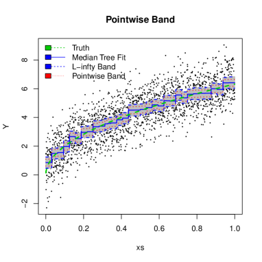
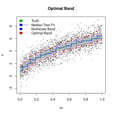
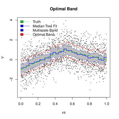
Figure 7: (Left) Pointwise $95\%$ credible intervals and $95\%$-$L^{\infty}$ credible intervals (gray area). (Right) Non-intersected multiscale $95\%$ credible band (77) obtained with $w_{l}=l^{1/2+0.01}$ (gray area) and the ‘optimal’ band (32) obtained with $v_{n}=1$. (Upper) The true function is $f_{0}(x)=2\sqrt{10x}$. (Lower) The true function is $f_{0}(x)=(4x-1)\mathbb{I}(x\leq 1/2)+(-2x+2)\mathbb{I}(x>1/2)$.

7.2 Numerical examples

We highlight the practicality of the confidence bands presented in Section 3.2 (and the following Section 7.3.5) on numerical examples. We implement Dyadic Bayesian CART as in [22] using the standard Metropolis-Hastings algorithm with a proposal distribution consisting of two steps: grow (splitting a randomly chosen bottom node) and prune (collapsing two children bottom nodes into one). The implementation is fairly straightforward due to immediate access to the posterior tree probabilities through a variant of (22) (these closed-form calculations can be easily updated for non-parametric regression).

We illustrate uncertainty quantification for $f_{0}$ using the intersection band (78) as well as the “optimal” band (32). The intersection construction yields exact asymptotic coverage; it uses up more posterior information and in this sense can be viewed as more Bayesian in spirit. Kolyan Ray [53], Section 6, implemented the intersection-credible set in the case of spike-and-slab priors and the white noise model. Here we provide an implementation in the regression model for tree priors. For the computation of the empirical median tree estimator in (69), one can easily identify nodes $(l,k)$ that have occurred in at least $50\%$ of posterior samples. Regarding the computation of $R_{n}$ in (77), the radius can be approximated using the $95\%$ quantile of the posterior samples of the multiscale norm $\|\cdot\|_{\mathcal{M}(w)}$–norm (acting on coefficients up to level $L_{max}$). Therefore, we see that while the confidence band in (78) may at first look computationally cumbersome, it can be readily obtained from posterior samples.

We generate $n=2^{11}$ observations from (64) with $f_{0}(x)=2\sqrt{10x}$ (top row in Figure 7) and $f_{0}(x)=(4x-1)\mathbb{I}(x\leq 1/2)+(-2x+2)\mathbb{I}(x>1/2)$ (bottom row in Figure 7). We choose $j_{0}(n)=4$ and $w_{l}=l^{1/2+\epsilon}$ (the multiscale weighting sequence) with $\epsilon=0.01$ and $\Gamma=1.01$ (the splitting probability parameter of the GW process prior). We run $2\,000$ iterations of the MH sampler with $500$ burnin samples. One tempting approach to uncertainty quantification is computing the pointwise $95\%$ credible intervals for each given $t_{i}$. These intervals are readily available from the posterior samples of the bottom node coefficients (transformed from the samples of the wavelet coefficients via the pinball formula (13)) and are portrayed in Figure 7 on the left (red dotted lines). For both functions $f_{0}$ these intervals are too narrow to uniformly capture $f_{0}$ (depicted in a green dashed line). For comparisons, we also plot the $95\%$–$L^{\infty}$–credible bands (blue dashed lines), which have better coverage. The $L^{\infty}$–band (gray area) is somewhat similar to the multiscale credible band but its coverage properties are not theoretically understood.

In comparison, the (not-intersected) multiscale $95\%$ credible band in (77) (Figure 7 on the right; gray area marked with blue dotted lines) is successful at containing the true function uniformly. These sets resemble the $L^{\infty}$–sets. Figure 7 plots the intersection band which has exact asymptotic coverage as well as the ‘optimal’ set (32) choosing $v_{n}=1$ (red dashed lines). Note, however, that this intersecting band is smaller than the band analyzed in Theorem 8 which yields even better coverage. The centering in Figure 7 (right) is the median tree estimator. Similarly as in [60], we have chosen the blow-up factor $v_{n}=1$ which yields a set (32) which contains the multiscale band. The intersection uses up substantial posterior information and stabilizes the construction. Out of curiosity, we tried different values $v_{n}$ and found that the choice $v_{n}=0.5$ roughly corresponds to the multiscale band.

7.3 Adaptive nonparametric BvM and applications

7.3.1 From $\|\cdot\|_{\infty}$ to BvM

Let us now formalize the notion of a nonparametric BvM theorem in multiscale spaces following [18] (we refer also to [17] for more background and discussion of the, different, $L^{2}$–type setting). Such spaces are defined through the speed of decay of multiscale coefficients $\beta_{lk}=\langle f,\psi_{lk}\rangle$. For a monotone increasing weighting sequence $w=(w_{l})_{l=0}^{\infty}$, with $w_{l}\geq 1$ and $w_{l}/\sqrt{l}\rightarrow\infty$ as $l\rightarrow\infty$ (such a $w=(w_{l})_{l=0}^{\infty}$ is called admissible) we define the following multiscale sequence space

$$\mathcal{M}(w)=\left\{x=(x_{lk}):\|x\|_{\mathcal{M}(w)}:=\sup_{l}\frac{\max_{k}|x_{lk}|}{w_{l}}<\infty\right\}.$$

We consider a separable closed subspace of $\mathcal{M}(w)$ defined as

$$\mathcal{M}_{0}(w)=\left\{x\in\mathcal{M}(w):\lim_{l\rightarrow\infty}\max_{k}\frac{|x_{lk}|}{w_{l}}=0\right\}.$$

Defining random variables $g_{lk}=\int_{0}^{1}\psi_{lk}(t)dW(t)\sim\mathcal{N}(0,1),$ according to Proposition 2 in [18], the Gaussian white noise $\mathbb{W}=(g_{lk})$ defines a tight Gaussian Borel measure in the space $\mathcal{M}_{0}(w)$ for admissible sequences $w$. The convergence in distribution of random variables in the multiscale space $\mathcal{M}_{0}(w)$ is metrised via the bounded Lipschitz metric $\beta_{\mathcal{M}_{0}(w)}$ defined below. For $\mu,\eta$ probability measures on a metric space $(S,d)$ define

$$\beta_{S}(\mu,\eta)=\sup_{F:\|F\|_{BL}\leq 1}\left|\int_{S}F(x)(d\mu(x)-d\eta(x))\right|,$$

$$\|F\|_{BL}=\sup_{x\in S}|F(x)|+\sup\limits_{x\neq y,x,y\in S}\frac{|F(x)-F(y)|}{d(x,y)}.$$

Denote with $\mathbb{X}=\mathbb{X}^{(n)}=(X_{lk}:l\in\mathbb{N}_{0},0\leq k<2^{l}),$ where $X_{lk}$ satisfy (2). Let $\widetilde{\Pi}_{n}=\Pi_{n}\circ\tau^{-1}_{\mathbb{X}}$ be the image measure of $\Pi(\cdot\,|\>X)$ under $\tau_{\mathbb{X}}:f\rightarrow\sqrt{n}(f-\mathbb{X}).$ Namely, for any Borel set $B$ we have

$$\widetilde{\Pi}_{n}(B)=\Pi\left(\sqrt{n}(f-\mathbb{X})\in B\,|\>X\right).$$ (74)

The following Theorem characterizes the adaptive nonparametric Bernstein-von Mises behavior of posteriors under the Bayesian Dyadic CART. In the result below, one assumes that trees sampled from $\Pi_{\mathbb{T}}$ contain all nodes $(j,k)$ for all $j\leq j_{0}(n)\to\infty$ slowly. Note that this constraint is easy to accommodate in the construction: for the GW process, one starts stopping splits only after depth $j_{0}(n)$, while for priors (5), it suffices to constrain the indicator $\mathbb{I}_{\mathcal{T}\in\mathbb{T}}$ to trees that fill all first $j_{0}(n)$ layers.

Theorem 9.

(Adaptive nonparametric BvM) Let $\mathcal{M}_{0}=\mathcal{M}_{0}(w)$ for some admissible sequence $w=(w_{l})$. Assume the Bayesian CART priors $\Pi_{\mathbb{T}}$ from Theorem 1 constrained to trees that fit $j_{0}(n)$ layers, i.e. $\gamma_{lk}=1$ for $l\leq j_{0}(n)$, for some strictly increasing sequence $j_{0}(n)\rightarrow\infty$ that satisfies $w_{j_{0}(n)}\geq c\,{\log n}$ for some $c>0$. Consider tree-shaped priors as in Theorem 1 (or using an $S$–regular wavelet basis, $S\geq 1$). Then the posterior distribution satisfies the weak Bernstein-von Mises phenomenon in $\mathcal{M}_{0}$ in the sense that

$$E_{f_{0}}\beta_{\mathcal{M}_{0}}(\widetilde{\Pi}_{n},\mathcal{N})\rightarrow 0\quad\text{as $n\rightarrow\infty$},$$

where $\mathcal{N}$ is the law of $\mathbb{W}$ in $\mathcal{M}_{0}$.

This result states an adaptive nonparametric BvM result, in the sense that the prior it considers also leads to an adaptive nonparametric convergence rate in $L^{\infty}$ (optimal up to log terms). It is only the second result of this kind after the one derived by Ray in [53]. This statement, proved in Section 12.3, can be shown, for example, by verifying the conditions in Proposition 6 of [18] (appropriate ‘tightness’ and convergence of finite dimensional distributions). The first tightness condition pertains to contraction in the $\mathcal{M}_{0}$–space, which can be obtained from our $\|\cdot\|_{\infty}$–results. In order to attain BvM, we need to modify the prior to always include a few coarsest dense layers in the tree (similarly as [53]). Such trees are semi-dense, where sparsity kicks in only deeper in the tree after $j_{0}(n)$ dense layers have already been fitted. This enables one to derive the convergence of finite dimensional distributions to suitable Gaussian distributions. For the independent wavelet prior, the last point follows easily from results in [17]. For the $g$–prior on trees corresponding to actual Bayesian CART, it requires a completely new argument based on the conditional posteriors given possible trees.

7.3.2 Application 1: multiscale confidence sets

First, let us consider multiscale credible balls for $f_{0}$, which we will use in the next subsection for refining the band construction used in the main paper. Such multiscale balls consist of functions $f$ that simultaneously satisfy multi-scale linear constraints (see e.g. (5) in [18]):

$$\mathcal{B}_{n}=\left\{f:\ \|f-\mathbb{X}\|_{\mathcal{M}(w)}\leq R_{n}/\sqrt{n}\right\},$$ (75)

where $R_{n}$ is chosen such that $\Pi[\mathcal{B}_{n}\,|\,X]=1-\gamma$ (or the smallest radius such that $\Pi[\mathcal{B}_{n}\,|\,X]\geq 1-\gamma$), i.e. $\mathcal{B}_{n}$ is a credible set of level $1-\gamma$.

Proposition 1.

Let $f_{0}\in\mathcal{H}_{M}^{\alpha}$ for some $\alpha\in(0,1],M>0$. Then for $\mathcal{B}_{n}$ as in (75),

$$P_{f_{0}}(f_{0}\in\mathcal{B}_{n})\rightarrow 1-\gamma,\qquad(\text{as }n\to\infty).$$

The proof of the Proposition 1 is a consequence of the fact that the nonparametric BvM in the multiscale space holds: one combines Theorem 9 and Theorem 5 in [18].

7.3.3 Application 2: BvM for functionals

As a second application of Theorem 9, we derive confidence bands for $F(t):=\int_{0}^{t}f(x)dx,0\leq t\leq 1$: those result from taking quantile credible bands in the following limiting distribution result. This application is described in Theorem 4 and the (short) proof is in Section 10.5.

7.3.4 Application 3: multiscale confidence bands in the white noise model

Let us first consider the case of the white noise model. For $R_{n}$ as in (75), $\sigma_{n}(X)$ as in (31) and $\widehat{f}_{T}$ as in (30), let us set

$$\mathcal{C}_{n}^{\mathcal{M}}=\left\{\,f:\ \|f-\mathbb{X}\|_{\mathcal{M}(w)}\leq R_{n}/\sqrt{n}\ ,\ \|f-\widehat{f}_{T}\|_{\infty}\leq\sigma_{n}(X)\,\right\}.$$ (76)

Let us recall the definition of the self-similarity class $\mathcal{H}_{SS}(\alpha,M,\varepsilon)$ from Definition 3.

Corollary 1.

Let $0<\alpha_{1}\leq\alpha_{2}\,\leq 1,\,M\geq 1,\,\gamma\in(0,1)$ and $\varepsilon>0$. Let the prior $\Pi$ and the sequence $(w_{l})$ be as in the statement of Theorem 9. Take $R_{n}$ as in (75), $\sigma_{n}$ as in (31) with $v_{n}$ such that $(\log{n})^{1/2}=o(v_{n})$ and let $\widehat{f}_{T}$ denote the median tree estimator (30). Then for $\mathcal{C}_{n}^{\mathcal{M}}$ defined in (76), uniformly over $\alpha\in[\alpha_{1},\alpha_{2}],$

$$\sup_{f_{0}\in\mathcal{H}_{SS}(\alpha,M,\varepsilon)}|P_{f_{0}}(f_{0}\in\mathcal{C}_{n}^{\mathcal{M}})-(1-\gamma)|\to 0,$$

as $n\to\infty$. In addition, for every $\alpha\in[\alpha_{1},\alpha_{2}]$ and uniformly over $f_{0}\in\mathcal{H}_{SS}(\alpha,M,\varepsilon)$, the diameter $|\mathcal{C}_{n}^{\mathcal{M}}|_{\infty}=\sup_{f,g\in\mathcal{C}_{n}^{\mathcal{M}}}\|f-g\|_{\infty}$ and the credibility of the band verify, as $n\to\infty$,

$$|\mathcal{C}_{n}^{\mathcal{M}}|_{\infty} =O_{P_{f_{0}}}((n/\log n)^{-\alpha/(2\alpha+1)}v_{n}),$$

$$\Pi[\mathcal{C}_{n}^{\mathcal{M}}\,|\,X] =1-\gamma+o_{P_{f_{0}}}(1).$$

This result states that by intersecting the confidence set $\mathcal{C}_{n}$ in (32) with the ball $\mathcal{B}_{n}$ from (75), one obtains a set with confidence (and credibility) at the prescribed level $1-\gamma$. It directly follows by applying Proposition 1 (which guarantees that $\mathcal{B}_{n}$ has confidence level $1-\gamma$ and hence also $\mathcal{C}_{n}^{\mathcal{M}}$, since $\mathcal{C}_{n}$ has confidence that goes to $1$) and the fact that by definition $\mathcal{B}_{n}$ has credibility $1-\gamma$ (and hence also $\mathcal{C}_{n}^{\mathcal{M}}$ asymptotically).

7.3.5 Application 4: multiscale confidence bands in regression

Now consider the regression setting (64). Let us define a discrete analogue for the multiscale confidence ball (75). Recall that in this setting the observations are the $Y$’s and that $X$ here denotes the matrix of $\psi_{lk}(t_{i})$’s as introduced in Section 7.1. Denote $\tilde{F}=(\tilde{f}_{T}(t_{i}))_{1\leq i\leq n}$ for $\tilde{f}_{T}$ the empirical median tree estimator. Set

$$\mathcal{B}_{n}^{b}=\{b=(b_{lk})_{l\leq L_{max},k}:\ \|b-X^{-1}\tilde{F}\|_{\mathcal{M}(w)}\leq R_{n}/\sqrt{n}\},$$ (77)

where $R_{n}$ is defined in such a way that $\Pi[\mathcal{B}_{n}^{b}\,|\,Y]=1-\gamma$ (or possibly $\geq 1-\gamma$) and where in slight abuse of notation $\|\cdot\|_{\mathcal{M}(w)}$ stands for the multiscale norm acting on coefficients up to level $L_{max}$ only (i.e. the supremum over $l$ in the definition of $\|\cdot\|_{\mathcal{M}(w)}$ is replaced by the maximum over $l\leq L_{max}$). For $\mathcal{C}_{n}^{e}$ as in (71), recalling the notation $F=(f(t_{i}))_{1\leq i\leq n}^{\prime}$, define

$$\tilde{}\mathcal{C}_{n}^{\mathcal{M}}=\mathcal{C}_{n}^{e}\cap\left\{f:\ X^{-1}F\in\mathcal{B}_{n}^{b}\right\}.$$ (78)

Corollary 2.

Consider a prior as in Theorem 9, and let $\mathcal{C}_{n}^{e}$ be constructed as in Theorem 8. For $\gamma>0$, let $\tilde{}\mathcal{C}_{n}^{\mathcal{M}}$ be defined as in (78). The set $\tilde{}\mathcal{C}_{n}^{\mathcal{M}}$ verifies the properties stated in Theorem 8 except that both confidence and credibility go to the nominal level $1-\gamma$ as $n\to\infty$.

This result is obtained in a similar way as for Corollary 1: first, one notes that a BvM result similar to Theorem 9 in white noise holds (details are omitted, the proof being similar). This implies that the ball $\mathcal{B}_{n}^{b}$ in (77) has confidence going to nominal level $1-\gamma$. One concludes by using Theorem 8, that ensures that $\mathcal{C}_{n}^{e}$, and then in turn $\tilde{}\mathcal{C}_{n}^{M}$, has the desired properties in terms of coverage, confidence and credibility.

7.4 Multi-dimensional extensions

Our tree-shaped wavelet reconstruction generalizes to the multivariable case, where a fixed number $d\geq 1$ of covariate directions are available for split. We outline one such generalization using the tensor product of Haar basis functions $\psi_{lk}$ from (3) defined as

$$\Psi_{l\boldsymbol{k}}(\boldsymbol{x}):=\psi_{lk_{1}}(x_{1})\cdots\psi_{lk_{d}}(x_{d})$$

for $l\geq 0$ and $\boldsymbol{k}=(k_{1},\ldots,k_{d})^{\prime}$ with $0\leq k_{i}\leq 2^{l}-1$ for $i=1,\ldots,d$, where $\Psi_{-1\boldsymbol{0}}(\boldsymbol{x})=\mathbb{I}_{(0,1]^{d}}(\boldsymbol{x})$. These wavelet tensor products can be associated with $d$-ary trees (as opposed to binary trees), where each internal node has $2^{d}$ children. The nodes in a $d$-ary tree satisfy a hierarchical constraint: $(l,\boldsymbol{k})\in\mathcal{T},l\geq 1\Rightarrow(l-1,\boldsymbol{\lfloor}\boldsymbol{k}/2\rfloor)\in\mathcal{T}$, where the floor operation is applied element-wise. This intuition can be gleaned from Figure 8 which organizes tensor wavelets with $l=0,1$ and $d=2$ in a flat $4$-ary tree.

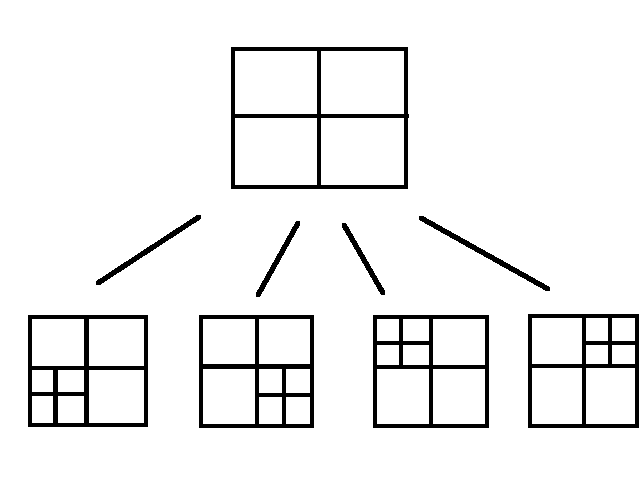
Figure 8: A plot of tensor Haar wavelets. The top figure plots $\Psi_{0\,(0,0)^{\prime}}$ and the bottom figures are $\Psi_{1\,(0,0)^{\prime}},\Psi_{0\,(1,0)^{\prime}},\Psi_{0\,(0,1)^{\prime}},\Psi_{0\,(1,1)^{\prime}}$ (from left to right).

We assume that $f_{0}$ belongs to $\alpha$-Hölder functions on $[0,1]^{d}$ for $0<\alpha\leq 1$ defined as

$$\mathcal{H}^{\alpha,d}_{M}:=\left\{f\in\mathcal{C}([0,1]^{d}):\|f\|_{\infty}+\sup_{\boldsymbol{x}\neq\boldsymbol{y}}\frac{|f(\boldsymbol{x})-f(\boldsymbol{y})|}{\|\boldsymbol{x}-\boldsymbol{y}\|^{\alpha}}\leq M\right\}.$$ (79)

The multiscale coefficients $\beta_{-1\boldsymbol{0}}={\langle}f_{0},\Psi_{-1\boldsymbol{0}}{\rangle}$ and

$$\beta_{l\boldsymbol{k}}={\langle}f_{0},\Psi_{l\boldsymbol{k}}{\rangle}=\int_{[0,1]^{d}}f_{0}(\boldsymbol{x})\Psi_{l\boldsymbol{k}}(\boldsymbol{x})\,d\boldsymbol{x}.$$

can be verified to satisfy, for some universal constant $C>0$,

$$|\beta_{l\boldsymbol{k}}|\leq C2^{-l(\frac{1}{2}+\alpha)d}.$$ (80)

Similarly as in Section 2.2, denoting with $\mathcal{T}_{int}^{\prime}$ the collection of internal nodes $(l,\boldsymbol{k})$ in a $d$-ary tree (including the node $(-1,\boldsymbol{0})$), one then obtains a wavelet reconstruction $f_{\mathcal{T},\boldsymbol{\beta}}(\boldsymbol{x})=\sum_{(l,\boldsymbol{k})\in\mathcal{T}_{int}^{\prime}}\beta_{l\boldsymbol{k}}\Psi_{l\boldsymbol{k}}(\boldsymbol{x})$, where coefficients $\beta_{l\boldsymbol{k}}$ can be assigned, for instance, a Gaussian independent product prior. There are several options for defining the $d$–dimensional version of the prior $\Pi_{\mathbb{T}}$. Restricting to Galton-Watson type priors, the most direct extension, for each node $(l,\boldsymbol{k})$ to be potentially split, either does not split it with probability $1-\Gamma^{-l}$, or splits it into $2^{d}$ children, leading to a full $2^{d}$–ary tree. Another, more flexible option, is to split $(l,\boldsymbol{k})$ into a random number of children inbetween $0$ and $2^{d}$, where a split in each specific direction occurs with probability $\Gamma^{-l}$, for $\Gamma$ a large enough constant.

Assuming that $d$ is fixed as $n\rightarrow\infty$, the general proving strategy of Theorem 1 can still be applied to conclude $\ell_{\infty}$–posterior convergence at the rate $\varepsilon_{n}=(\log n/n)^{\alpha/(2\alpha+d)}\log^{\delta}n$ for some $\delta>0$. The proof requires the threshold $\mathcal{L}_{c}$ in (45) to be modified as satisfying $2^{\mathcal{L}_{c}}\asymp(n/\log n)^{1/(2\alpha+d)}$.

The basis we consider here is a tensor product where, within each tree layer, splits occur along each direction simultaneously. This is not necessarily what Bayesian CART does in practice. Multivariate Bayesian CART can be more transparently translated using anisotropic Haar wavelet basis functions which more closely resemble recursive partitioning (as explained in [28]). Our approach extends more naturally to the tensor product basis, but it could be in principle applied to other basis functions such as this one.

8 Basic Lemmata

8.1 Properties of the pinball matrix (14)

While $A_{\mathcal{T}}^{\prime}A_{\mathcal{T}}$ is not proportional to an identity matrix (for trees other than flat trees), it does have a nested sparse structure which will be exploited in our analysis.

Proposition 2.

Denote with $(l_{1},k_{1})$ the deepest rightmost internal node in the tree $\mathcal{T}$, i.e. the node $(l,k)\in\mathcal{T}_{int}$ with the highest index $2^{l}+k$. Let $\mathcal{T}^{-}$ be a tree obtained from $\mathcal{T}$ by turning $(l_{1},k_{1})$ into a terminal node. Then

$$A_{\mathcal{T}}^{\prime}A_{\mathcal{T}}=\left(\begin{matrix}A_{\mathcal{T}^{-}}^{\prime}A_{\mathcal{T}^{-}}+\boldsymbol{v}\boldsymbol{v}^{\prime}&\boldsymbol{0}\\ \boldsymbol{0}^{\prime}&2^{l_{1}+1}\end{matrix}\right)$$ (81)

for a vector of zeros $\boldsymbol{0}\in\mathbb{R}^{|\mathcal{T}_{ext}|-1}$ and a vector $\boldsymbol{v}\in\mathbb{R}^{|\mathcal{T}_{ext}|-1}$ obtained from $A_{\mathcal{T}}$ by first deleting its last column and then transposing the last row of this reduced matrix.

Proof.

The index $(l_{1},k_{1})$, by definition, corresponds to the last entry in the vector $\boldsymbol{\beta}_{\mathcal{T}}$. We note that $\mathcal{T}^{-}_{int}=\mathcal{T}_{int}\backslash\{(l_{1},k_{1})\}$ and $\mathcal{T}^{-}_{ext}=\mathcal{T}_{ext}\backslash\{(l_{1}+1,2k_{1}),(l_{1}+1,2k_{1}+1)\}\cup\{(l_{1},k_{1})\}$. The matrix $A_{\mathcal{T}^{-}}$ can be obtained from $A_{\mathcal{T}}$ by deleting the last column of $A_{\mathcal{T}}$ and then deleting the last row, further denoted with $\boldsymbol{v}^{\prime}$. The desired statement (81) is obtained by noting that the last column of $A_{\mathcal{T}}$ (associated with $\beta_{l_{1},k_{1}})$ is orthogonal to all the other columns. This is true because (a) this column has only two nonzero entries that correspond to the last two siblings $\{(l_{1}+1,2k_{1}),(l_{1}+1,2k_{1}+1)\}$, (b) the last two rows of $A_{\mathcal{T}}$ differ only in the sign of the last entry because $\{(l_{1}+1,2k_{1}),(l_{1}+1,2k_{1}+1)\}$ are siblings and share the same ancestry with the same weights up to the sign of their immediate parent. Finally, the entry $2^{l_{1}+1}$ follows from (13). ∎

Corollary 3.

Under the prior (17), the coefficient $\beta_{lk}$ of any internal node $(l,k)$ which has terminal descendants is independent of all the remaining internal coefficients.

Proof.

Follows directly from Prop. 2 after reordering the nodes. ∎

The following proposition characterizes the eigenspectrum of $A_{\mathcal{T}}^{\prime}A_{\mathcal{T}}$ which will be exploited in our proofs.

Proposition 3.

The eigenspectrum of $A_{\mathcal{T}}^{\prime}A_{\mathcal{T}}$ consists of the diagonal entries of $\boldsymbol{D}=\mathrm{diag}(\widetilde{d}_{lk,lk})=A_{\mathcal{T}}A_{\mathcal{T}}^{\prime}$ in (15). Moreover, the diagonal entries $\mathrm{diag}(A_{\mathcal{T}}^{\prime}A_{\mathcal{T}})=\{d_{lk,lk}\}_{lk\in\mathcal{T}_{int}}$ satisfy $d_{-10,-10}=|\mathcal{T}_{ext}|$ and $d_{lk,lk}=\sum_{j=l+1}^{d(\mathcal{T})}2^{j}\sum_{m=0}^{2^{j-1}}\mathbb{I}[\beta_{lk}\in[(0,0)\leftrightarrow(j,m)]_{\mathcal{T}}]$ with $[(0,0)\leftrightarrow(l,k)]_{\mathcal{T}}:=\{(0,0),(1,\lfloor k/2^{l-1}\rfloor),\dots,(l-1,\lfloor k/2\rfloor)\}.$

Proof.

The first statement follows from (15) and the fact that $A_{\mathcal{T}}^{\prime}A_{\mathcal{T}}$ and $A_{\mathcal{T}}A_{\mathcal{T}}^{\prime}$ have the same spectrum, and the second statement from (13). ∎

8.2 Other lemmata

Lemma 4.

Assume that a square matrix $A$ is diagonally dominant by rows (i.e., $a_{kk}>\sum_{j\neq k}|a_{kj}|$). Then

$$\|A\|_{\infty}<\frac{1}{\min_{k}(|a_{kk}|-\sum_{j\neq k}|a_{kj}|)}.$$

Proof.

Theorem 1 in Varah [62]. ∎

Lemma 5.

For an invertible matrix $M\in\mathbb{R}^{p\times p}$ and $\boldsymbol{v}\in\mathbb{R}^{p}$ we have

$$(M^{-1}+\boldsymbol{v}\boldsymbol{v}^{\prime}/g_{n})^{-1}=M-\frac{M\boldsymbol{v}\boldsymbol{v}^{\prime}M}{g_{n}+\boldsymbol{v}^{\prime}M\boldsymbol{v}}\quad\text{for $g_{n}>0$}.$$

Proof.

Follows immediately by direct computation.∎

Lemma 6.

Let $\mathbb{C}_{K}$ denote the number of full binary trees with $K+1$ leaves. Then

$$\mathbb{C}_{K}=\frac{(2K)!}{(K+1)!K!}\asymp 4^{K}/K^{3/2}.$$

Proof.

The number $\mathbb{C}_{K}$ is the Catalan number (see e.g. [59]), which verifies the identity. The second assertion follows from Stirling’s formula. ∎

Lemma 7.

Let $\boldsymbol{Y}\sim\mathcal{N}_{K}(\boldsymbol{\mu},\Sigma)$ be a Gaussian random vector. Denote with $\{\sigma_{i}\}_{i=1}^{K}=\mathrm{diag}(\Sigma)$, with $\bar{\mu}=\max\limits_{1\leq i\leq K}\mu_{i}$ and with $\bar{\sigma}^{2}=\max\limits_{1\leq i\leq K}\sigma^{2}_{i}$ the maximal mean and variance. Then

$$\mathbb{E\,}\left[\max_{1\leq i\leq K}|Y_{i}|\right]\leq\bar{\mu}+\sqrt{2\,\bar{\sigma}^{2}\log K}+2\sqrt{2\pi\bar{\sigma}^{2}}.$$ (82)

Proof.

We start by noting that $|Y_{i}|\leq\bar{\mu}+|Y_{i}-\mu_{i}|$. Next, one can use the formula, valid for any real $\mu_{i}$, $c>0$ and real random variables $Y_{i}$,

$$\mathbb{E\,}[\max_{1\leq i\leq K}|Y_{i}-\mu_{i}|]\leq c+\sum_{i=1}^{K}\int_{c}^{\infty}\mathbb{P}(|Y_{i}-\mu_{i}|>x)dx.$$ (83)

Assuming the Gaussian distribution, the integral is of order $\int_{c}^{\infty}2\mathrm{e}^{-x^{2}/2\sigma_{i}^{2}}dx$
$\leq\,\sqrt{2\pi\sigma_{i}^{2}}\,\mathrm{e}^{-c^{2}/2\sigma^{2}_{i}}$. Then (82) follows from (83) by choosing $c=\sqrt{2\bar{\sigma}^{2}\log K}$. ∎

Lemma 8 (see, e.g., [26]).

For a positive integer $d$, let $\mu,\mu_{1},\mu_{2}\in\mathbb{R}^{d}$ and let $\Sigma,\Sigma_{1},\Sigma_{2}$ be positive definite $d\times d$ matrices. Then the exist universal constants $C_{1},C_{2}>0$ such that, for TV the total variation distance,

$$TV\left(\mathcal{N}(\mu,\Sigma_{1}),\mathcal{N}(\mu,\Sigma_{2})\right) \leq C_{1}\|\Sigma_{1}^{-1}\Sigma_{2}-I_{d}\|_{F}$$

$$TV\left(\mathcal{N}(\mu_{1},\Sigma),\mathcal{N}(\mu_{2},\Sigma)\right) \leq C_{2}\frac{\|\mu_{1}-\mu_{2}\|^{2}}{\sqrt{(\mu_{1}-\mu_{2})^{\prime}\Sigma(\mu_{1}-\mu_{2})}},$$

where $\|\cdot\|_{F}$ denotes the Frobenius norm.

Proof.

The first inequality follows from Theorem 1.1 in [26] and the second by Theorem 1.2 in [26] (by setting $\Sigma=\Sigma_{1}=\Sigma_{2}$ in their statement). ∎

9 Non-dyadic Bayesian CART: properties and examples

9.1 Basic properties and examples

Lemma 9.

For a set $A$ of admissible nodes $(l,k)$ as above, let us define $\beta_{lk}^{B}=\langle f,\psi_{lk}^{B}\rangle$, where $\psi_{lk}^{B}$ is the unbalanced Haar wavelet in (39) and where $f\in\mathcal{H}^{\alpha}_{M}$ was defined in (24). Then

$$|\beta_{lk}^{B}|\leq M2^{-1/2}\max\{|L_{lk}|,|R_{lk}|\}^{\alpha+1/2}.$$ (84)

Proof.

Let us denote by $\bar{C}\equiv 1/\sqrt{|L_{lk}|^{-1}+|R_{lk}|^{-1}}$. We have

$$|\beta_{lk}^{B}| =\left|\bar{C}\left\{\int_{L_{lk}}\frac{f(x)}{|L_{lk}|}dx-\int_{R_{lk}}\frac{f(x)}{|R_{lk}|}dx\right\}\right|$$

$$\leq\frac{\bar{C}}{|L_{lk}|}\int_{0}^{|L_{lk}|}\left|{f(x+l_{lk})}-f\left(b_{lk}+x\frac{|R_{lk}|}{|L_{lk}|}\right)\right|dx.$$

Next, from $\alpha$-Hölder continuity (24), we have

$$\left|{f(x+l_{lk})}-f\left(b_{lk}+x\frac{|R_{lk}|}{|L_{lk}|}\right)\right|\leq M\left||L_{lk}|+x\left(\frac{|R_{lk}|}{|L_{lk}|}-1\right)\right|^{\alpha}.$$

Since $\bar{C}\leq 2^{-1/2}\max\{|L_{lk}|,|R_{lk}|\}^{1/2}$ we have

$$|\beta_{lk}^{B}|\leq M\bar{C}\max\{|L_{lk}|,|R_{lk}|\}^{\alpha}\leq M2^{-1/2}\max\{|L_{lk}|,|R_{lk}|\}^{\alpha+1/2}.$$

This follows from the fact that for $x\in(0,|L_{lk}|)$ we have

$$M\left||L_{lk}|+x\left(\frac{|R_{lk}|}{|L_{lk}|}-1\right)\right|^{\alpha}\leq\max\{|L_{lk}|,|R_{lk}|\}^{\alpha}.\qed$$

For the classical Haar basis (3), one obtains (23) from (84) by noting $\max\{|L_{lk}|,|R_{lk}|\}=2^{-(l+1)}$. [32] points out that the computational complexity of the discrete UH transform could be unnecessarily large and imposes the balancing requirement $\max\left\{|L_{lk}|,|R_{lk}|\right\}\leq E(|L_{lk}|+|R_{lk}|)\ \forall(l,k)\in A$, for some $1/2\leq E<1$. In order to control the combinatorial complexity of the basis system, we also require that the UH wavelets are not too imbalanced. To this end, we introduce the notion of weakly balanced wavelets in Section 4.1. A graphical depiction of the unbalanced Haar wavelets for certain non-dyadic choices of split points $b_{lk}$ are in Figure 9.

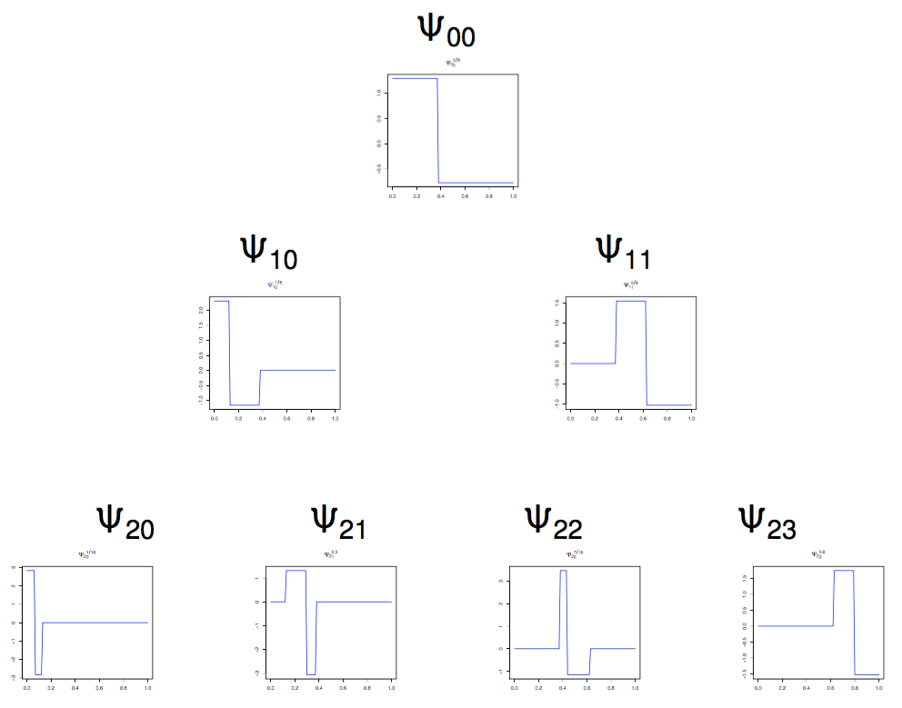
Figure 9: Diagram of unbalanced (right) Haar wavelets for $l\leq 2$.

Example 3.

To glean insights into the balancing condition (40), we first consider an example of UH system which is not weakly balanced for some given $n,D$, say $n=2^{4}$ and $D=2$. If we choose $b_{00}=1/2$, $b_{10}=1/2-1/n$ and $b_{11}=3/4$, we have

$$L_{10} =(0,1/2-1/n], R_{10} =(1/2-1/n,1/2],$$

$$L_{11} =(1/2,3/4], R_{11} =(3/4,1].$$

While the node $(1,1)$ is seen to satisfy (40) with $E=5$, we note that $\max\{|L_{10}|,|R_{10}|\}=(n-2)/(2n)=7/16.$ However, $7/16$ cannot be written as $M_{10}/2^{D+1}=M_{10}/8$ for any integer $M_{10}$. This is why the split points $b_{00},b_{10}$ and $b_{11}$ do not belong to any weakly balanced UH wavelet system with balancing constant $D=2$. Weakly balanced systems can be built by choosing splits in such a way that the “granularity” does not increase too rapidly throughout the branching process. With granularity $R(l,\Psi_{A}^{B})$ of the $l^{th}$ layer we mean the smallest integer $R\geq 1$ such that $\min_{0\leq k<2^{l}}\min\{|L_{lk}|,|R_{lk}|\}=j/2^{R}$ for some $j\in\{1,2,\dots,2^{R-1}\}$. For instance, setting $D=2$ and $E=3$ one can build weakly balanced wavelets by first picking $b_{00}$ from values $\{\frac{1}{4},\frac{1}{2},\frac{3}{4}\}$. If, e.g. $b_{00}=3/4$ (i.e. $R(0,\Psi_{A}^{B})=2$), the next split $b_{10}$ can be selected from $\{\frac{1}{4},\frac{3}{8},\frac{1}{2}\}$, while $b_{11}$ has to be set as $7/8$.

Our theoretical development relies in part on combinatorial properties of weakly balanced UH systems and on the speed of decay of the multiscale functionals $\beta_{lk}^{B}=\langle f,\psi_{lk}^{B}\rangle$ as the layer index $l\in\mathbb{N}$ increases. These two fundamental properties are encapsulated in Lemma 11 which is vital to the proof of Theorem 6.

9.2 Granularity lemma

Lemma 10.

Denote with $\Psi_{A}^{B}$ a weakly balanced UH system according to Definition 5. Then for any $(l,k){\in A}$,

$$\min\{|L_{lk}|,|R_{lk}|\}=\frac{m_{lk}}{2^{l+D}}\quad\text{ for some}\quad m_{lk}\in\{1,\dots,C+l\}.$$

Proof.

We prove the statement by induction. First, from the definition of weak balancedness, we have $\min\{|L_{00}|,|R_{00}|\}=1-M_{00}/2^{D}=j/2^{D}$ (for $j=2^{D}-M_{00}$) and by definition this is less than $M_{00}/2^{D}\leq C/2^{D}$, so $j\leq C$. Assume now that the statement holds for $l-1\geq 0$ and consider a node $(l,k){\in A}$ for some $0\leq k<2^{l}$. The union $L_{lk}\cup R_{lk}$ is either $L_{l-1\,\lfloor k/2\rfloor}$ or $R_{l-1\,\lfloor k/2\rfloor}$; without loss of generality, suppose it is $R_{l-1\,\lfloor k/2\rfloor}$. Then, from weak balancedness, we find

$$\min\{|L_{lk}|,|R_{lk}|\}=|R_{l-1\,\lfloor k/2\rfloor}|-M_{lk}/2^{l+D}.$$ (85)

If $|R_{l-1\,\lfloor k/2\rfloor}|\leq|L_{l-1\,\lfloor k/2\rfloor}|$, we use induction to find $|R_{l-1\,\lfloor k/2\rfloor}|=j_{1}/2^{l-1+D}$ for some $j_{1}\in\{1,\dots,C+l-1\}$ and thereby (85) equals $j/2^{l+D}$ for $j=2j_{1}-M_{lk}$. As this is at most $M_{lk}/2^{l+D}=\max\{|L_{lk}|,|R_{lk}|\}$, one deduces $M_{lk}\geq j_{1}$ and then $j/2^{l+D}\leq j_{1}/2^{l+D}$ with $j_{1}\leq C+l-1\leq C+l$. If $|R_{l-1\,\lfloor k/2\rfloor}|>|L_{l-1\,\lfloor k/2\rfloor}|$, we again use weak balancedness to write (85) as $j/2^{l+D}$ with $j=2M_{l-1\,\lfloor k/2\rfloor}-M_{lk}\leq M_{lk}$, using again $M_{lk}/2^{l+D}=\max\{|L_{lk}|,|R_{lk}|\}$, so that $j$ is again less than $C+l$. The result follows by induction. ∎

9.3 Complexity lemma

Lemma 11.

Consider a weakly balanced UH wavelet system $\Psi_{A}^{B}=\{\Psi_{lk}^{B}:(l,k)\in A\}$ according to (40) and let $f\in\mathcal{H}^{\alpha}_{M}$. Then the following conditions hold for $\delta=3$, with constants independent of $B$: for any $(l,k)\in A$

1. the basis function $\psi_{lk}^{B}$ can be expressed as a linear combination of at most $C_{0}l^{\delta}$ Haar functions $\psi_{jk}$ for $j\leq l+D$ and some $C_{0}>0$, and

2. there exists $C_{1}>0$ (depending only on $E,D$ from (40)) such that $|\beta_{lk}^{B}|\leq{C_{1}M}l^{\delta/2}2^{-l(\alpha+1/2)}$.

Proof.

First, the function $\psi_{lk}^{B}$ belongs to $\text{Vect}\{\mathbb{I}_{I_{(l+D)m}}:0\leq m<2^{l+D}\}$ and the support of $\psi_{lk}^{B}$ spans at most $2(E+l)$ of the indicators $\mathbb{I}_{I_{(l+D)m}}$. These indicators can be expressed in terms of at most $l+D$ of $\psi_{lk}$’s (one per level above $l+D$), which yields an upper bound $2(E+l)(l+D)\asymp l^{2}$ and thereby (B1) with $\delta=2$. Second, the balancing condition (40) gives $\max\{|L_{lk}|,|R_{lk}|\}\leq(E+l)2^{-l-D}$ which, combined with Lemma 9 implies

$$|\beta_{lk}^{B}|\leq M2^{\alpha-1}(E+l)^{\alpha+1/2}2^{-(l+D)(\alpha+1/2)}\leq C_{1}Ml^{3/2}2^{-l(\alpha+1/2)},$$

by taking the worst case $\alpha=1$, which proves (B2) with $\delta=3$. ∎

9.4 The quantile example

Lemma 12.

The quantile system $\Psi_{A}^{B}$ from Example 2 is weakly balanced in the sense of Definition 5 for balancing constants satisfying $E=2+3\,C_{q}2^{D-1}$, where $\|1/g\|_{\infty}\leq C_{q}$ and $\|g\|_{\infty}<2^{D-1}/(2E)$.

Proof.

Let us start by writing explicitly the intervals $L_{lk},R_{lk}$. Assuming without loss of generality that $k$ is odd, i.e. $(l,k)$ is the right child node,

$$|L_{lk}| =b_{lk}-b_{(l-1)\lfloor k/2\rfloor}=G_{L_{max}+D}^{-1}[(2k+1)/2^{l+1}]-G_{L_{max}+D}^{-1}[(2\lfloor k/2\rfloor+1)/2^{l}],$$

$$|R_{lk}| =b_{(l-2)\lfloor k/4\rfloor}-b_{lk}=G_{L_{max}+D}^{-1}[(2\lfloor k/4\rfloor+1)/2^{l-1}]-G_{L_{max}+D}^{-1}[(2k+1)/2^{l+1}].$$

We first show by contradiction that $\max\{|L_{lk}|,|R_{lk}|\}\geq E/2^{l+D}$ for $E\geq 1$. Let us denote $y_{1}=G^{-1}[(2k+1)/2^{l+1}]$, $y_{2}=G^{-1}[(2\lfloor k/2\rfloor+1)/2^{l}]$ and $y_{3}=G^{-1}[(2\lfloor k/4\rfloor+1)/2^{l-1}]$. Assuming $|L_{lk}|<E/2^{l+D}$, one obtains

$$\lfloor 2^{L_{max}+D}y_{1}\rfloor-\lfloor 2^{L_{max}+D}y_{2}\rfloor<E2^{L_{max}-l},$$

and thereby $y_{1}-y_{2}<E2^{-l-D+1}.$ Next, using the fact that $k$ is odd,

$$\frac{1}{2^{l+1}} =|(2k+1)/2^{l+1}-(2\lfloor k/2\rfloor+1)/2^{l}|$$

$$=|G(y_{1})-G(y_{2})|\leq\|g\|_{\infty}|y_{1}-y_{2}|\leq\|g\|_{\infty}2E2^{-l-D},$$

which yields a contradiction when $\|g\|_{\infty}<2^{D-1}/(2E)$. Similarly, when $|R_{lk}|<E/2^{l+D}$, one obtains

$$1/2^{l+1} <|(2k+1)/2^{l+1}-(2\lfloor k/4\rfloor+1)/2^{l-1}|$$

$$=|G(y_{3})-G(y_{1})|\leq\|g\|_{\infty}|y_{3}-y_{1}|<\|g\|_{\infty}2E\,3\,2^{-l-D}.$$

Next, we note that for $\|1/g\|_{\infty}\leq C_{q}$ and $E:=\left(2+3\,C_{q}2^{D-1}\right)$,

$$|R_{lk}| =\frac{1}{2^{L_{max}+D}}\left[\lfloor 2^{L_{max}+D}y_{1}\rfloor-\lfloor 2^{L_{max}+D}y_{3}\rfloor\right]$$

$$\leq\frac{2}{2^{L_{max}+D}}+\left\|\frac{1}{g}\right\|_{\infty}\frac{3}{2^{l+1}}\leq\frac{E}{2^{l+D}}.$$

Similarly, one obtains $|L_{lk}|<E/2^{l+D}$, which concludes that the quantile system is weakly balanced.∎

10 Remaining proofs for Section 3

10.1 Proof of Theorem 1: remaining settings

In this section, we provide the proof of Theorem 1 under more general prior settings. We consider different tree priors $\Pi_{\mathbb{T}}(\mathcal{T})$ from Section 2.1 (i.e. the conditionally uniform prior in (5) and the exponential-type prior mentioned in Extension 2). In addition, we consider the prior

$$\pi(\boldsymbol{\beta}_{\mathcal{T}})\sim\mathcal{N}(0,\Sigma_{\mathcal{T}})$$ (86)

with $\Sigma_{\mathcal{T}}=g_{n}(A_{\mathcal{T}}^{\prime}A_{\mathcal{T}})^{-1}$ (the $g$-prior) as well as more general covariance structures $\Sigma_{\mathcal{T}}$ that satisfy

$$\lambda_{min}(\Sigma_{\mathcal{T}})\gtrsim 1/\sqrt{\log n}\quad\text{and}\quad\lambda_{max}(\Sigma_{\mathcal{T}})\lesssim n^{a}\quad\text{for some $a>0$}.$$ (87)

First, we show that Lemma 1 holds under this setting.

10.1.1 Proof of Lemma 1 (general setting)

Recall the ratio (48) from Section 6.1

$$\frac{W_{X}(\mathcal{T})}{W_{X}(\mathcal{T}^{-})} =\frac{\Pi_{\mathbb{T}}(\mathcal{T})}{\Pi_{\mathbb{T}}(\mathcal{T}^{-})}\frac{\sqrt{|I+n\Sigma_{\mathcal{T}^{-}}|}}{\sqrt{|I+n\Sigma_{\mathcal{T}}|}}\frac{\mathrm{e}^{n^{2}\boldsymbol{X}_{\mathcal{T}}^{\prime}(nI+\Sigma_{\mathcal{T}}^{-1})^{-1}\boldsymbol{X}_{\mathcal{T}}/2}}{\mathrm{e}^{n^{2}\boldsymbol{X}_{\mathcal{T}^{-}}^{\prime}(nI+\Sigma_{\mathcal{T}^{-}}^{-1})^{-1}\boldsymbol{X}_{\mathcal{T}^{-}}/2}}.$$ (88)

The $g$-prior. We first focus on bounding this ratio assuming $\Sigma_{\mathcal{T}}=g_{n}\,(A_{\mathcal{T}}^{\prime}A_{\mathcal{T}})^{-1}$. Proposition 2 implies

$$nI_{K}+\Sigma_{\mathcal{T}}^{-1}=\left(\begin{matrix}nI_{K-1}+\Sigma_{\mathcal{T}^{-}}^{-1}+\frac{1}{g_{n}}\boldsymbol{v}\boldsymbol{v}^{\prime}&\boldsymbol{0}\\ \boldsymbol{0}^{\prime}&n+\frac{2^{l_{1}+1}}{g_{n}}\\ \end{matrix}\right),$$ (89)

where the vector $\boldsymbol{v}\in\mathbb{R}^{|\mathcal{T}_{ext}|-1}$ (defined in Proposition 2) is obtained from $A_{\mathcal{T}}$ by first deleting its last column and then transposing the last row of this reduced matrix. Using the determinant formula $|A+\boldsymbol{u}\boldsymbol{u}^{\prime}|=|A|(1+\boldsymbol{u}^{\prime}A^{-1}\boldsymbol{u})$ for $A$ invertible (see Lemma 1.1 in [27]), and setting $M=(nI_{K-1}+\Sigma_{\mathcal{T}^{-}}^{-1})^{-1}$, one gets

$$\frac{{|nI_{K-1}+\Sigma_{\mathcal{T}^{-}}^{-1}|}}{{|nI_{K}+\Sigma_{\mathcal{T}}^{-1}|}}=\frac{1}{(n+2^{l_{1}+1}/g_{n})\left[1+\boldsymbol{v}^{\prime}M\boldsymbol{v}\right/g_{n}]}<\frac{1}{(n+2^{l_{1}+1}/g_{n})}.$$ (90)

Using again the determinant formula and Proposition 2, we can write

$$\frac{{|\Sigma_{\mathcal{T}^{-}}|}}{{|\Sigma_{\mathcal{T}}|}}=\frac{|A_{\mathcal{T}}^{\prime}A_{\mathcal{T}}|}{|A_{\mathcal{T}^{-}}^{\prime}A_{\mathcal{T}^{-}}|}=\frac{2^{l_{1}+1}}{g_{n}}\left(1+\boldsymbol{v}^{\prime}(A_{\mathcal{T}^{-}}^{\prime}A_{\mathcal{T}^{-}})^{-1}\boldsymbol{v}\right)\leq\frac{2^{l_{1}+1}}{g_{n}}\left(1+2^{l_{1}}\right).$$

The inequality above uses two facts. First, we have $\|\boldsymbol{v}\|_{2}^{2}=1+\sum_{l=0}^{l_{1}-1}2^{l}=2^{l_{1}}$ which follows from the definition of $\boldsymbol{v}$ which describes its entries as amplitudes of the Haar wavelets in the ancestry of the deepest rightmost internal node $(l_{1},k_{1})$ (using the notation from Lemma 1). Second, from Proposition 3 we have $\lambda_{max}[(A_{\mathcal{T}^{-}}^{\prime}A_{\mathcal{T}^{-}})^{-1}]=1/\lambda_{min}(A_{\mathcal{T}^{-}}^{\prime}A_{\mathcal{T}^{-}})\leq 1$. Indeed, Proposition 3 (combined with (15)) shows that the smallest eigenvalue of $A_{\mathcal{T}}^{\prime}A_{\mathcal{T}}$ equals $2^{d}$ where $d$ is the depth of the most shallow leaf node in $\mathcal{T}_{ext}$. Let us now set

$$D:=\boldsymbol{X}_{\mathcal{T}}^{\prime}(nI+\Sigma_{\mathcal{T}}^{-1})^{-1}\boldsymbol{X}_{\mathcal{T}}-\boldsymbol{X}_{\mathcal{T}^{-}}^{\prime}(nI+\Sigma_{\mathcal{T}^{-}}^{-1})^{-1}\boldsymbol{X}_{\mathcal{T}^{-}}.$$ (91)

Combining with (89), it follows from a variant of the Sherman–Morrison’s matrix inversion formula (Lemma 5) that

$$(nI_{K}+\Sigma_{\mathcal{T}}^{-1})^{-1}=\left(\begin{matrix}M-\frac{M\boldsymbol{v}\boldsymbol{v}^{\prime}M}{g_{n}+\boldsymbol{v}^{\prime}M\boldsymbol{v}}&\boldsymbol{0}\\ \boldsymbol{0}^{\prime}&1/(n+2^{l_{1}+1}/g_{n})\\ \end{matrix}\right),$$

from which one deduces that

$$D= \frac{X_{l_{1}k_{1}}^{2}}{n+2^{l_{1}+1}/g_{n}}-\frac{\boldsymbol{X}_{\mathcal{T}^{-}}^{\prime}M\boldsymbol{v}\boldsymbol{v}^{\prime}M\boldsymbol{X}_{\mathcal{T}^{-}}}{g_{n}+\boldsymbol{v}^{\prime}M\boldsymbol{v}}<\frac{X_{l_{1}k_{1}}^{2}}{n+2^{l_{1}+1}/g_{n}}.$$ (92)

Since for $l_{1}>\mathcal{L}_{c}$ we have $2X_{l_{1}k_{1}}^{2}\leq 5\log n/n$, we can write

$$\frac{W_{X}(\mathcal{T})}{W_{X}(\mathcal{T}^{-})}\frac{\Pi_{\mathbb{T}}(\mathcal{T}^{-})}{\Pi_{\mathbb{T}}(\mathcal{T})}{<}\sqrt{\frac{2^{l_{1}+1}\left(1+2^{l_{1}}\right)}{g_{n}(n+2^{l_{1}+1}/g_{n})}}\mathrm{e}^{\frac{X_{l_{1}k_{1}}^{2}n^{2}}{2(n+2^{l_{1}+1}/g_{n})}}<\sqrt{\frac{2^{2(l_{1}+1)}}{ng_{n}}}n^{5/4}.$$

For $g_{n}=n$, and for $\mathcal{T}\in\mathbb{T}_{d}$, so that $2^{l_{1}}\lesssim 2^{d}$, the last display is bounded by a constant times ${n^{-1/4}2^{d}p_{d}}$, and the argument can be completed in similar vein as before, with now $\Pi[d(\mathcal{T})>\mathcal{L}_{c}\,|\,X]=o_{P}(1)$ if ${\Gamma>2\mathrm{e}^{5}}$.

General Covariance $\Sigma_{\mathcal{T}}$. We now show how the proof can be modified by assuming a general covariance matrix $\Sigma_{\mathcal{T}}$ on the internal wavelet coefficients. Recall again the ratio (48) from Section 6.1. We use the Cauchy’s interlace theorem for eigenvalues of Hermitian matrices which states that the eigenvalues of a principal submatrix are interlaced within eigenvalues of the original matrix (Theorem 8.1.7 of [39]). Since $\Sigma_{\mathcal{T}^{-}}$ is a $(K-1)\times(K-1)$ dimensional submatrix of a $(K\times K)$ dimensional matrix $\Sigma_{\mathcal{T}}$, we have (denoting with $\lambda_{l}(\Sigma)$ the $l^{th}$ largest eigenvalue of $\Sigma$)

$$\lambda_{1}(\Sigma_{\mathcal{T}})\geq\lambda_{1}(\Sigma_{\mathcal{T}^{-}})\geq\lambda_{2}(\Sigma_{\mathcal{T}})\geq\cdots\geq\lambda_{K-1}(\Sigma_{\mathcal{T}})\geq\lambda_{K-1}(\Sigma_{\mathcal{T}^{-}})\geq\lambda_{K}(\Sigma_{\mathcal{T}})$$

and thereby

$$\frac{|I+n\Sigma_{\mathcal{T}^{-}}|}{|I+n\Sigma_{\mathcal{T}}|}=\frac{\prod_{l=1}^{K-1}[1+n\lambda_{l}(\Sigma_{\mathcal{T}^{-}})]}{\prod_{l=1}^{K}[1+n\lambda_{l}(\Sigma_{\mathcal{T}})]}\leq\frac{1}{1+n\lambda_{min}(\Sigma_{\mathcal{T}})}.$$

Using the matrix inversion formula $(I+B)^{-1}=I-(I+B^{-1})^{-1}$ (a variant of Sherman-Morrison-Woodbury formula), we get

$$(nI+\Sigma_{\mathcal{T}}^{-1})^{-1}=\frac{1}{n}\left[I-(I+n\Sigma_{\mathcal{T}})^{-1}\right]$$

and thereby

$$\boldsymbol{X}_{\mathcal{T}}^{\prime}(nI+\Sigma_{\mathcal{T}}^{-1})^{-1}\boldsymbol{X}_{\mathcal{T}}=\frac{1}{n}\|\boldsymbol{X}_{\mathcal{T}}\|_{2}^{2}-\frac{1}{n}\boldsymbol{X}_{\mathcal{T}}^{\prime}(I+n\Sigma_{\mathcal{T}})^{-1}\boldsymbol{X}_{\mathcal{T}}.$$

Writing $\boldsymbol{X}_{\mathcal{T}}=(\boldsymbol{X}_{\mathcal{T}^{-}},X_{l_{1}k_{1}})^{\prime}$, where $(l_{1},k_{1})$ it the deepest rightmost internal node in $\mathcal{T}$ (as in Section 6.1), and using the definition of $D$ in (91), we have

$$D =\frac{X_{l_{1}k_{1}}^{2}}{n}-\frac{1}{n}\left[\boldsymbol{X}_{\mathcal{T}}^{\prime}(I+n\Sigma_{\mathcal{T}})^{-1}\boldsymbol{X}_{\mathcal{T}}-\boldsymbol{X}_{\mathcal{T}^{-}}^{\prime}(I+n\Sigma_{\mathcal{T}^{-}})^{-1}\boldsymbol{X}_{\mathcal{T}^{-}}\right]$$

$$<\frac{X_{l_{1}k_{1}}^{2}}{n}\left(1-\frac{1}{1+n\lambda_{max}(\Sigma_{\mathcal{T}})}\right)$$

$$\qquad\qquad+\frac{\|\boldsymbol{X}_{\mathcal{T}^{-}}\|_{2}^{2}}{n}\left(\frac{1}{1+n\lambda_{min}(\Sigma_{\mathcal{T}^{-}})}-\frac{1}{1+n\lambda_{max}(\Sigma_{\mathcal{T}})}\right).$$

This inequality follows from the fact that

$$\boldsymbol{X}_{\mathcal{T}}^{\prime}(I+n\Sigma_{\mathcal{T}})^{-1}\boldsymbol{X}_{\mathcal{T}}\geq\|\boldsymbol{X}_{\mathcal{T}}\|_{2}^{2}\lambda_{min}[(I+n\Sigma_{\mathcal{T}})^{-1}]=\frac{\|\boldsymbol{X}_{\mathcal{T}^{-}}\|_{2}^{2}+X_{l_{1}k_{1}}^{2}}{1+n\lambda_{max}(\Sigma_{\mathcal{T}})}.$$

It follows from the proof of Lemma 1 that $X_{l_{1}k_{1}}^{2}\lesssim\log n/n$ and $\|\boldsymbol{X}_{\mathcal{T}^{-}}\|_{2}^{2}\leq C_{1}$ (as was shown in (94)). Moreover, from our assumption (86) we have $\lambda_{min}(\Sigma_{\mathcal{T}^{-}})\geq 1/\sqrt{\log n}$ and thereby

$$\frac{W_{X}(\mathcal{T})}{W_{X}(\mathcal{T}^{-})} <\sqrt{\frac{\log n}{n}}\frac{\Pi_{\mathbb{T}}(\mathcal{T})}{\Pi_{\mathbb{T}}(\mathcal{T}^{-})}\exp\left\{\frac{nX_{l_{1}k_{1}}^{2}}{2}+\frac{n\|\boldsymbol{X}_{\mathcal{T}^{-}}\|_{2}^{2}}{2(1+n\lambda_{min}(\Sigma_{\mathcal{T}^{-}}))}\right\}$$

$$<\frac{\Pi_{\mathbb{T}}(\mathcal{T})}{\Pi_{\mathbb{T}}(\mathcal{T}^{-})}\mathrm{e}^{C_{2}\log n}.$$

Proceeding as in the proof of Lemma 1, one can show (46) for a suitably large $\Gamma>0$.

Other Tree Priors $\Pi_{\mathbb{T}}(\mathcal{T})$. The only modification needed to carry over the proof to the other two priors is the bound for the ratio $\Pi_{\mathbb{T}}(\mathcal{T})/\Pi_{\mathbb{T}}(\mathcal{T}^{-})$. Consider the conditionally uniform prior from Section 2.1.1 defined in (5). Denoting $K=|\mathcal{T}_{ext}|$ and $\mathbb{C}_{K}$ the number of full binary trees with $K+1$ leaves, we have

$$\frac{\Pi_{\mathbb{T}}(\mathcal{T})}{\Pi_{\mathbb{T}}(\mathcal{T}^{-})}=\frac{\pi(K)}{\pi(K-1)}\frac{\mathbb{C}_{K-1}}{\mathbb{C}_{K-2}},$$

and Lemma 6 now implies, for a universal constant $C>0$,

$$\frac{\Pi_{\mathbb{T}}(\mathcal{T})}{\Pi_{\mathbb{T}}(\mathcal{T}^{-})}\lesssim\frac{\lambda}{K}\frac{4^{K-1}(K-2)^{3/2}}{4^{K-2}(\{K-1\}\vee 1)^{3/2}}\leq C\lambda/K.$$

Choosing $\lambda=1/n^{c}$ for some $c>7/4$, it follows that

$$\Pi[d(\mathcal{T})>\mathcal{L}_{c}\,|\,X]\leq 4\,\lambda\,n^{3/4}\sum_{d=\mathcal{L}_{c}+1}^{L}{2^{d}}/K\leq 4\,\lambda\,n^{3/4}{2^{L}}\rightarrow 0.$$

Finally, for the exponential-type prior mentioned in Extension 2), one has $\Pi_{\mathbb{T}}(\mathcal{T})/\Pi_{\mathbb{T}}(\mathcal{T}^{-})=1/n^{c}$, so one can argue similarly.

10.1.2 Proof of Lemma 2 (general setting)

We recall the ratio

$$\frac{W_{X}(\mathcal{T})}{W_{X}(\mathcal{T}^{+})}=\frac{\Pi_{\mathbb{T}}(\mathcal{T})}{\Pi_{\mathbb{T}}(\mathcal{T}^{+})}\prod_{j=0}^{s}\frac{N_{X}(\mathcal{T}^{(j-1)})}{N_{X}(\mathcal{T}^{(j)})}.$$ (93)

in (53) and find an upper bound assuming different priors.

The $g$-prior. We now modify the proof of Lemma 2 for the $g$-prior obtained with $\Sigma_{\mathcal{T}}=g_{n}(A_{\mathcal{T}}^{\prime}A_{\mathcal{T}})^{-1}$. Denoting with $K_{j}=|\mathcal{T}^{(j)}_{ext}|$ and because $\mathcal{T}^{(j-1)}$ is obtained from $\mathcal{T}^{(j)}$ by removing two children nodes (or, equivalently, an internal node $X_{l_{j}k_{j}}$), we can apply Proposition 2 to obtain the following upper bound for $N_{X}(\mathcal{T}^{(j-1)})/N_{X}(\mathcal{T}^{(j)})$. Namely, going back to (91) and (92), we invoke again the matrix determinant lemma $|A+\boldsymbol{u}\boldsymbol{u}^{\prime}|=|A|(1+\boldsymbol{u}^{\prime}A^{-1}\boldsymbol{u})$ and the matrix inversion lemma (Lemma 5) as in (90) to obtain

$$\frac{N_{X}(\mathcal{T}^{(j-1)})}{N_{X}(\mathcal{T}^{(j)})}\leq \sqrt{\frac{(g_{n}n+2^{l_{j}+1})(g_{n}+\boldsymbol{v}^{\prime}M\boldsymbol{v})}{g_{n}^{2}}}$$

$$\times\exp\left\{-\frac{n^{2}\,X_{l_{j}k_{j}}^{2}}{2(n+2^{l_{j}+1}/g_{n})}+n^{2}\frac{\boldsymbol{X}_{\mathcal{T}^{(j-1)}}^{\prime}M\boldsymbol{v}\boldsymbol{v}^{\prime}M\boldsymbol{X}_{\mathcal{T}^{(j-1)}}}{2(g_{n}+\boldsymbol{v}^{\prime}M\boldsymbol{v})}\right\},$$

where $M=(nI_{K_{j-1}}+\Sigma^{-1}_{\mathcal{T}^{(j-1)}})^{-1}$ for $\boldsymbol{v}\in\mathbb{R}^{|\mathcal{T}^{(j-1)}|}$ which depends on $\mathcal{T}^{(j-1)}$ according to Proposition 2. Next, for $C>0$ a large enough constant and $l_{j-1}$ the depth of the deepest internal node in $\mathcal{T}^{(j-1)}$,

$$\|\boldsymbol{X}_{\mathcal{T}^{(j-1)}}\|_{2}^{2} \leq X_{-10}^{2}+\sum_{l=0}^{l_{j-1}}\sum_{k=0}^{2^{l}-1}X_{lk}^{2}\leq C\left[1+\sum_{l=0}^{l_{j-1}}\left(2^{-2\,l\,\alpha}+\frac{2^{l}}{n}\,\log n\right)\right]\leq C_{4}.$$ (94)

Moreover, using the fact that $\boldsymbol{v}^{\prime}MM\boldsymbol{v}=\boldsymbol{v}^{\prime}M^{1/2}M^{1/2}M\boldsymbol{v}\leq\lambda_{max}(M)\boldsymbol{v}^{\prime}M\boldsymbol{v}$ we obtain

$$\boldsymbol{X}_{\mathcal{T}^{(j-1)}}^{\prime}M\boldsymbol{v}\boldsymbol{v}^{\prime}M\boldsymbol{X}_{\mathcal{T}^{(j-1)}} \leq\|\boldsymbol{X}_{\mathcal{T}}^{(j-1)}\|^{2}_{2}\lambda_{max}(M\boldsymbol{v}\boldsymbol{v}^{\prime}M)\leq\|\boldsymbol{X}_{\mathcal{T}}^{(j-1)}\|^{2}_{2}\mathrm{tr}(M\boldsymbol{v}\boldsymbol{v}^{\prime}M)$$

$$\leq\|\boldsymbol{X}_{\mathcal{T}}^{(j-1)}\|^{2}_{2}\boldsymbol{v}^{\prime}MM\boldsymbol{v}\leq\|\boldsymbol{X}_{\mathcal{T}}^{(j-1)}\|^{2}_{2}\lambda_{max}(M)\boldsymbol{v}^{\prime}M\boldsymbol{v},$$

and

$$\lambda_{\max}(M)=\frac{1}{n+\lambda_{min}(A_{\mathcal{T}^{(j-1)^{\prime}}}A_{\mathcal{T}^{(j-1)}})/g_{n}}<\frac{1}{n},$$

one can write

$$n^{2}\frac{\boldsymbol{X}_{\mathcal{T}^{(j-1)}}^{\prime}M\boldsymbol{v}\boldsymbol{v}^{\prime}M\boldsymbol{X}_{\mathcal{T}^{(j-1)}}}{2(g_{n}+\boldsymbol{v}^{\prime}M\boldsymbol{v})} <\frac{n^{2}\|\boldsymbol{X}_{\mathcal{T}^{(j-1)}}\|_{2}^{2}\lambda_{max}(M)}{2g_{n}/(\boldsymbol{v}^{\prime}M\boldsymbol{v})+2}\leq\frac{n^{2}C_{4}\|\boldsymbol{v}\|_{2}^{2}\lambda_{max}^{2}(M)}{2g_{n}}$$

$$\leq C_{4}\frac{2^{l_{j}}}{2g_{n}},$$

where we used the fact that $\|\boldsymbol{v}\|_{2}^{2}=2^{l_{j}}$ (as explained previously in Section 10.1.1). Finally, because $X^{2}_{l_{s}k_{s}}\geq C_{5}A^{2}\log^{2}n/n$ for some $C_{5}>0$ we use the above bounds in the expression (93) to obtain

$$\prod_{j=0}^{s}\frac{N_{X}(\mathcal{T}^{(j-1)})}{N_{X}(\mathcal{T}^{(j)})} <\left(\frac{n(g_{n}+2)}{g_{n}}\right)^{s+1}\exp\left\{C_{4}\sum_{j=0}^{s}\frac{2^{l_{j}-1}}{g_{n}}-\frac{nC_{5}A^{2}\log^{2}n}{2(n+2^{{l_{j}}+1}/g_{n})}\right\}$$

$$<\exp\left\{(s+1)\log(3n)+C_{4}\frac{(s+1)2^{l_{s}-1}}{g_{n}}-C_{5}A^{2}\log^{2}n/{2}\right\}.$$

With $g_{n}=n$, the exponent is dominated by the last term. One then proceeds with (53) as before in the proof of Lemma 2.

General Covariance $\Sigma_{\mathcal{T}}$. We again deploy the interlacing eigenvalue theorem in the expression (53) to obtain the following upper bound for $\frac{N_{X}(\mathcal{T}^{(j-1})}{N_{X}(\mathcal{T}^{(j)})}$ (using matrix determinant and inversion lemmata as before)

$$\sqrt{1+n\lambda_{\max}(\Sigma_{\mathcal{T}^{(j)}})}\exp\left\{-\frac{nX_{l_{j}k_{j}}^{2}}{2}\frac{n\lambda_{min}(\Sigma_{\mathcal{T}^{(j)}})}{1+n\lambda_{min}(\Sigma_{\mathcal{T}^{(j)}})}+\frac{n\|\boldsymbol{X}_{\mathcal{T}^{(j-1)}}\|_{2}^{2}}{2(1+n\lambda_{min}(\Sigma_{\mathcal{T}^{(j)}}))}\right\}.$$

Using the expression (53) and assumptions $\lambda_{max}(\Sigma_{\mathcal{T}})\lesssim n^{a}$ for some $a\geq 1$ and $\lambda_{min}(\Sigma_{\mathcal{T}^{(j)}})\geq 1/\sqrt{\log n}$, we obtain for $C_{2},C_{3}>0$

$$\frac{W_{X}(\mathcal{T})}{W_{X}(\mathcal{T}^{+})}<\frac{\Pi_{\mathbb{T}}(\mathcal{T})}{\Pi_{\mathbb{T}}(\mathcal{T}^{+})}\exp\left\{C_{2}(s+1)\sqrt{\log n}-C_{3}A^{2}\log^{2}n\right\}.$$

Using this bound, one can proceed as in the proof of Lemma 2 and show (118).

Other Tree Priors $\Pi_{\mathbb{T}}(\mathcal{T})$. As before, the only modification needed is the bound for $\Pi_{\mathbb{T}}(\mathcal{T})/\Pi_{\mathbb{T}}(\mathcal{T}^{+})$. Denote by $K^{+}=|\mathcal{T}^{+}_{ext}|$ and $K=|\mathcal{T}_{ext}|$ and note that $K^{+}-K=l_{s}-l_{0}$. For the conditionally uniform prior from Section 2.1.1 we then have

$$\frac{\Pi_{\mathbb{T}}(\mathcal{T})}{\Pi_{\mathbb{T}}(\mathcal{T}^{+})} =\lambda^{-(l_{s}-l_{0})}\frac{K^{+}!\mathbb{C}_{K^{+}-1}}{K!\mathbb{C}_{K-1}}\lesssim\left(\frac{\lambda}{4}\right)^{-(l_{s}-l_{0})}\frac{(K^{+})!}{K!}$$

$$\lesssim\left(\frac{\lambda}{4}\right)^{-(l_{s}-l_{0})}{\mathrm{e}^{(l_{s}-l_{0})\{1+\log[K+(l_{s}-l_{0})]\}}}.$$

With $\lambda=n^{-c}$ and $K\leq 2^{\mathcal{L}_{c}+1}$, this is bounded from above by $C\mathrm{e}^{C\,\log^{2}n}$ for some $C>0$ and the proof is completed as before. For the exponential-type prior, one similarly uses $\Pi_{\mathbb{T}}(\mathcal{T})/\Pi_{\mathbb{T}}(\mathcal{T}^{+})=\mathrm{e}^{c(l_{s}-l_{0})\log n}\leq\mathrm{e}^{c\log^{2}n}.$

10.1.3 Proof of Lemma 3 (general setting)

We now show the proof of Lemma 3 for the $g$-prior with $\Sigma_{\mathcal{T}}=g_{n}(A_{\mathcal{T}}^{\prime}A_{\mathcal{T}})^{-1}$ and a general covariance matrix under the assumptions (87). Recall expressions (58) and (59) in Section 6.3 and the fact that $(I+B)^{-1}=I-(I+B^{-1})^{-1}$ which yields $n\widetilde{\Sigma}_{\mathcal{T}}-I_{K}=-(I_{K}+n\Sigma_{\mathcal{T}})^{-1}$ for $\widetilde{\Sigma}_{\mathcal{T}}=(nI_{K}+\Sigma_{\mathcal{T}}^{-1})^{-1}$ (recalling that $K=|\mathcal{T}_{ext}|\leq n$). Focusing on the $g$-prior, we have $\lambda_{max}(\widetilde{\Sigma}_{\mathcal{T}})<1/n$ and (using Proposition 3 which yields $\lambda_{max}(A_{\mathcal{T}}^{\prime}A_{\mathcal{T}})<2^{d}\leq n$ where $d$ is the depth of the deepest node)

$$\lambda_{max}(I_{K}+n\Sigma_{\mathcal{T}})^{-1}<\lambda_{max}(A_{\mathcal{T}}^{\prime}A_{\mathcal{T}})/(ng_{n})<1/g_{n}.$$

Assuming $g_{n}=n$ we can thus write

$$\|(n\widetilde{\Sigma}_{\mathcal{T}}-I_{K})\boldsymbol{\beta}_{\mathcal{T}}^{0}\|_{\infty}\leq\frac{\|\boldsymbol{\beta}_{\mathcal{T}}^{0}\|_{\infty}\sqrt{K}}{1+n\lambda_{min}(\Sigma_{\mathcal{T}})}\leq\frac{C\sqrt{K}\lambda_{max}(A_{\mathcal{T}}^{\prime}A_{\mathcal{T}})}{n\,g_{n}}\leq C/\sqrt{n}.$$ (95)

Next, we note that $\widetilde{\Sigma}_{\mathcal{T}}^{-1}$ is strictly diagonally dominant. Indeed, with $g_{n}=n$ we have $\widetilde{\Sigma}_{\mathcal{T}}^{-1}=nI_{K}+\frac{1}{g_{n}}A_{\mathcal{T}}^{\prime}A_{\mathcal{T}}$ and

$$\frac{1}{g_{n}}\|A_{\mathcal{T}}^{\prime}A_{\mathcal{T}}\|_{\infty}\leq\frac{\sqrt{K}}{g_{n}}\lambda_{max}(A_{\mathcal{T}}^{\prime}A_{\mathcal{T}})<\sqrt{n},$$

where $\|A\|_{\infty}=\max\limits_{1\leq i\leq m}\sum_{j=1}^{n}|a_{ij}|$ is defined as the maximum absolute row sum of an $(m\times n)$ matrix $A$. Writing $A_{\mathcal{T}}^{\prime}A_{\mathcal{T}}=(a_{ij})_{i,j}^{K,K}$, it then follows from Lemma 4 (Theorem 1 in [62]) that

$$\|\widetilde{\Sigma}_{\mathcal{T}}\|_{\infty}\leq\frac{1}{n+\frac{1}{g_{n}}\min\limits_{1\leq k\leq K}\Delta_{k}},\quad\text{where}\quad\Delta_{k}=|a_{kk}|-\sum_{j\neq k}|a_{kj}|.$$ (96)

Since $\Delta_{k}/g_{n}>-\frac{1}{g_{n}}\|A_{\mathcal{T}}^{\prime}A_{\mathcal{T}}\|_{\infty}>-\sqrt{n}$ and using the fact that $\|\boldsymbol{\varepsilon}_{\mathcal{T}}\|_{\infty}\lesssim\sqrt{\log n}$ on the event $\mathcal{A}$, we obtain

$$\sqrt{n}\|\widetilde{\Sigma}_{\mathcal{T}}\boldsymbol{\varepsilon}_{\mathcal{T}}\|_{\infty}\leq\sqrt{n}\|\widetilde{\Sigma}_{\mathcal{T}}\|_{\infty}\|\boldsymbol{\varepsilon}_{\mathcal{T}}\|_{\infty}\lesssim\sqrt{\frac{\log n}{n}}.$$ (97)

The sum of the remaining two terms in (58) can be bounded by a multiple of $\sqrt{\log n/n}$ by noting that $\bar{\sigma}^{2}\leq\|\widetilde{\Sigma}_{\mathcal{T}}\|_{\infty}\lesssim 1/n.$ The statement (57) then follows from (58).

For the general covariance matrix $\Sigma_{\mathcal{T}}$ we find (similarly as in (95)) that when $\lambda_{min}(\Sigma_{\mathcal{T}})\geq 1/\sqrt{\log n}$ we have $\|(n\widetilde{\Sigma}_{\mathcal{T}}-I_{K})\boldsymbol{\beta}^{0}_{\mathcal{T}}\|_{\infty}\leq C\sqrt{\log n/n}.$ Next, because

$$\|\Sigma^{-1}_{\mathcal{T}}\|_{\infty}\leq\sqrt{K}\lambda_{max}(\Sigma_{\mathcal{T}}^{-1})\leq\sqrt{K\log n}<\sqrt{n\log n}$$

the matrix $\widetilde{\Sigma}_{\mathcal{T}}=(nI_{K}+\Sigma_{\mathcal{T}}^{-1})^{-1}$ is diagonally dominant and thereby (using Lemma 4)

$$\|\widetilde{\Sigma}_{\mathcal{T}}\|_{\infty}\leq\frac{1}{n+\min\limits_{1\leq k\leq K}\Delta_{k}}\quad\text{where}\quad\Delta_{k}=|\sigma_{kk}|-\sum_{j\neq k}|\sigma_{kj}|$$

and where $\Sigma_{\mathcal{T}}^{-1}=(\sigma_{jk})_{j,k=1}^{K,K}$. Since $\Delta_{k}>-\sqrt{n\log n}$ for all $k=1,\dots,K$, the inequalities (97) and (57) hold.

10.1.4 End of proof of Theorem 1 (general setting)

The rest of the proof can now be completed using similar arguments as in Section 6.4.

10.2 Smooth wavelets

The strategy of the proof of Theorem 1 can be directly applied for an $S$–regular wavelet basis. Similar to [18], Section 2, one updates the index set $l\geq 0,0\leq k<2^{l}$ for the Haar basis in the definition of the ball (23) as follows: the index sets becomes $l\geq J_{0}-1,k=0,\ldots,2^{l}-1$, for $J_{0}=J_{0}(S)$ large enough, and one denotes the usual “scaling function” $\varphi$ as the first wavelet $\psi_{(J_{0}-1)0}$. The proof is then the same (up to a multicative constant depending on the chosen basis) as in the Haar basis case, up to replacing the ‘localisation’ identity $\|\sum_{k}|\psi_{lk}|\|_{\infty}=2^{l/2}$ in the Haar basis case by the ‘localisation’ inequality $\|\sum_{k}|\psi_{lk}|\|_{\infty}\leq C2^{l/2}$, with $C$ depending on the chosen basis only.

10.3 Proof of Theorem 2: exact rate

Proof.

Define a sequence

$$L^{*}=\left\lceil\log_{2}\left[M^{1/(\alpha+1/2)}\left(n/\log^{2}n\right)^{1/(2\alpha+1)}\right]\right\rceil,$$

so that $2^{L^{*}}\asymp(n/\log^{2}{n})^{1/(2\alpha+1)}$. Define the sequence of functions $f_{0}^{n}$ (below we write simply $f_{0}$ for simplicity) by its sequence of wavelet coefficients as follows: set all coefficients $\beta_{lk}^{0}$ to $0$ except for $\beta_{L^{*}0}^{0}=M2^{-L^{*}(1/2+\alpha)}$. By definition, $f_{0}$ belongs to $\mathcal{H}(\alpha,M)$. Let us also note that if $(L^{*},0)$ does not belong to the tree $\mathcal{T}$, one can bound from below

$$\ell_{\infty}(f_{\mathcal{T},\boldsymbol{\beta}},f_{0})\geq 2^{L^{*}/2}|\beta_{L^{*}0}|=M2^{-L^{*}\alpha}\geq C^{\prime}\varepsilon_{n}.$$

So, to prove the result, it is enough to show that $\Pi[(L^{*},0)\notin\mathcal{T}_{int}\,|\>X]\rightarrow 1$, i.e. the node $(L^{*},0)$ does not belong to a tree sampled from the posterior with probability going to $1$, or equivalently, if $\mathbb{T}_{L^{*}0}$ denotes the set of all full binary trees (of depth at most $L_{max}$) that contain $(L^{*},0)$ as an internal node, that $\Pi[\mathbb{T}_{L^{*}0}\,|\,X]=o_{P}(1)$. To prove this, let us consider a given tree $\mathcal{T}\in\mathbb{T}_{L^{*}0}$. As it contains the node $(L^{*},0)$, it must also contain all nodes $(\lambda,0)$ with $0\leq\lambda\leq L^{*}$, in particular $(L_{1},0)$, where $L_{1}=\lceil L^{*}/2\rceil$, say. We note that $L^{*}\asymp L^{*}-L_{1}\asymp\log{n}$. Let $\tau^{*}$ be the maximal subtree of $\mathcal{T}$ that has $(L_{1},0)$ as its root. Next, let $\mathcal{T}^{*}_{-}$ denote the remainder tree built from $\mathcal{T}$ by erasing all of $\tau^{*}$ except for the node $(L_{1},0)$ (so that $\mathcal{T}^{*}_{-}$ still has a full-binary tree structure). So, $\mathcal{T}^{*}_{-}$ and $\tau^{*}$ have only the node $(L_{1},0)$ in common, and the union of their nodes gives the original tree $\mathcal{T}$. Let us now write

$$\Pi[\mathbb{T}_{L^{*}0}\,|\,X]=\frac{\sum_{\mathcal{T}\in\mathbb{T}_{L^{*}0}}W_{X}(\mathcal{T})}{\sum_{\mathcal{T}\in\mathbb{T}}W_{X}(\mathcal{T})}=\frac{\sum_{\mathcal{T}\in\mathbb{T}_{L^{*}0}}\frac{W_{X}(\mathcal{T})}{W_{X}(\mathcal{T}^{*}_{-})}W_{X}(\mathcal{T}^{*}_{-})}{\sum_{\mathcal{T}\in\mathbb{T}}W_{X}(\mathcal{T})}.$$

Let ${q=q(\tau^{*})}$ denote the number of internal nodes $\tau^{*}_{int}$ of the subtree $\tau^{*}$. From the Galton-Watson prior, we obtain

$$\frac{\Pi_{\mathbb{T}}[\mathcal{T}]}{\Pi_{\mathbb{T}}[\mathcal{T}^{*}_{-}]}=\prod_{(l,k)\in\tau^{*}_{int}}p_{l}\prod_{(l,k)\in\tau^{*}_{ext}}(1-p_{l})\frac{1}{1-p_{L_{1}}}\leq 2\prod_{(l,k)\in\tau^{*}_{int}}\Gamma^{-l}.$$ (98)

Then, by definition of $\mathcal{T}_{-}^{*}$ and $\tau^{*}$,

$$\frac{W_{X}(\mathcal{T})}{W_{X}(\mathcal{T}^{*}_{-})} =\frac{\Pi_{\mathbb{T}}(\mathcal{T})}{\Pi_{\mathbb{T}}(\mathcal{T}^{*}_{-})}\prod_{(l,k)\in\tau^{*}_{int}}\frac{\exp\{(n+1)X_{lk}^{2}/2\}}{\sqrt{n+1}}$$

$$\leq 2(n+1)^{-q/2}\cdot\prod_{(l,k)\in\tau^{*}_{int}}\Gamma^{-l}\exp\{(n+1)X_{lk}^{2}/2\}.$$ (99)

We bound the data-dependent part in the previous line by using $(a+b)^{2}\leq 2a^{2}+2b^{2}$. Furthermore, noting that the noise variables $|\varepsilon_{lk}|$ are uniformly bounded for $l+1\leq L_{max},0\leq k<2^{l},$ by $2\log{n}$ on an event of overwhelming probability, we can upper-bound $(n+1)\sum_{(l,k)\in\tau^{*}_{int}}X_{lk}^{2}/2$ by

$$(n+1)\sum_{(l,k)\in\tau^{*}_{int}}\left[(\beta_{L^{*}0}^{0})^{2}\mathbb{I}_{(l,k)=(L^{*},0)}+\frac{1}{n}\max_{l+1\leq L_{max},k}\varepsilon_{lk}^{2}\right]$$

$$\leq(n+1)(\beta_{L^{*}0}^{0})^{2}+2\frac{n+1}{n}(\log{n})q\leq\frac{n+1}{n}\log^{2}{n}+2\frac{n+1}{n}(\log{n})q.$$

Now, using that for $(l,k)\in\tau^{*}_{int}$, we have $l\geq L_{1}\geq\frac{1}{2\alpha+1}\log_{2}\left(\frac{M^{2}n}{\log n}\right)=:c(\alpha,M,n)$, one notes that

$$\sum_{(l,k)\in\tau^{*}_{int}}l\geq\max\Big{(}c(\alpha,M,n)q,\sum_{l=L_{1}}^{L^{*}}l\Big{)}\geq c(\alpha,M,n)\max\left(q,\frac{3}{2}c(\alpha,M,n)\right),$$

which is bounded from below by $c(\alpha,M,n)q$, where we have used that $q\geq L^{*}-L_{1}+1\geq L_{1}\geq c(\alpha,M,n)$ and $L_{1}+L^{*}>3c(\alpha,M,n)$. One then deduces that the product of terms $\Gamma^{-l}$ dominates (99), as long as $\log(\Gamma)$ is large enough (noting also that $1/(2\alpha+1)\geq 1/(2S+1)$), in the control of $W_{X}(\mathcal{T})/W_{X}(\mathcal{T}_{-}^{*})$. That is, for some constant $C>0$,

$$\frac{W_{X}(\mathcal{T})}{W_{X}(\mathcal{T}_{-}^{*})}\leq\exp\{-C(\log{n})q\}=:b_{q},$$

where the last bound only depends on the number of internal nodes $q$ of $\tau^{*}$. By coming back to the above bound on the posterior $\Pi[\mathbb{T}_{L^{*}0}\,|\,X]$, let us split the sum on the numerator as follows. Let $\mathbb{T}_{L^{*}0}^{q}$ denote the set of trees $\mathcal{T}=\mathcal{T}_{-}^{*}\cup\tau^{*}$ in $\mathbb{T}_{L^{*}0}$ such that $|\tau_{int}^{*}|=q$. Then $\Pi[\mathbb{T}_{L^{*}0}\,|\,X]$ is bounded by

$$\sum_{q\geq 1}\frac{\sum_{\mathcal{T}\in\mathbb{T}_{L^{*}0}^{q}}b_{q}W_{X}(\mathcal{T}_{-}^{*})}{\sum_{\mathcal{T}\in\mathbb{T}}W_{X}(\mathcal{T})}\leq\sum_{q\geq 1}\frac{\sum_{\mathcal{T}_{1}\in\mathbb{T}_{-}^{*q}}a_{q}b_{q}W_{X}(\mathcal{T}_{1})}{\sum_{\mathcal{T}_{1}\in\mathbb{T}_{-}^{*q}}W_{X}(\mathcal{T}_{1})},$$

where $\mathbb{T}_{-}^{*q}$ denotes the set of all possible $\mathcal{T}^{*}_{-}$ that can be obtained from $\mathcal{T}\in\mathbb{T}_{L^{*}0}^{q}$ and where $a_{q}$ denotes the number of different possible trees $\tau^{*}$ such that $|\tau_{int}^{*}|=q$. To obtain the last bound, we also used that each $\mathcal{T}\in\mathbb{T}_{L^{*}0}$ is uniquely caracterised by a pair $(\mathcal{T}_{-}^{*},\tau^{*})$, so that the sum over $\mathcal{T}$ can be rewritten as a double sum over $\mathcal{T}_{-}^{*}$ and $\tau^{*}$. One deduces that, as $q$ cannot be larger than $2^{L}$,

$$\Pi[\mathbb{T}_{L^{*}0}\,|\,X]\leq\sum_{q=1}^{2^{L}}a_{q}b_{q}.$$

As $a_{q}$ is less (because of the restriction $|\mathcal{T}|\leq L$) or equal to the number of full binary trees with $q$ internal nodes, i.e. with $2q+1$ nodes in total, we have $a_{q}\leq\mathbb{C}_{2q}$, which is bounded from above by $4^{2q}$ by Lemma 6. We conclude that $\Pi[\mathbb{T}_{L^{*}0}\,|\,X]$ is bounded above by $\exp(-C\log^{2}{n})$ for some $C>0$, on an event of overwhelming probability, which concludes the proof for the Galton-Watson prior. Similarly, for the exponential prior, we replace (98) directly with

$$\frac{\Pi_{\mathbb{T}}[\mathcal{T}]}{\Pi_{\mathbb{T}}[\mathcal{T}_{-}^{*}]}\propto\mathrm{e}^{-c(|\mathcal{T}_{ext}|-|\mathcal{T}^{*}_{-ext}|)\log n}=\mathrm{e}^{-c\,q\log n},$$

where we used the fact that $|\mathcal{T}_{ext}|-|\mathcal{T}^{*}_{-ext}|=|\tau^{*}_{ext}|-1=|\tau^{*}_{int}|=q$. For the conditionally uniform prior, we have for $\lambda=1/n^{c}$ for some $c>0$

$$\frac{\Pi_{\mathbb{T}}[\mathcal{T}]}{\Pi_{\mathbb{T}}[\mathcal{T}_{-}^{*}]}=\frac{\pi(|\mathcal{T}_{ext}|)}{\pi(|\mathcal{T}^{*}_{-ext}|)}\frac{\mathbb{C}_{|\mathcal{T}^{*}_{-int}|}}{\mathbb{C}_{|\mathcal{T}_{int}|}}\lesssim\lambda^{q}\mathrm{e}^{-q\log|\mathcal{T}_{ext}|}\lesssim\mathrm{e}^{-c\,q\log n},$$

and the end of the proof is then the same as for the GW prior. ∎

10.4 Proof of Theorem 3: confidence bands

In the proof, we repeatedly use the properties of the median tree $\mathcal{T}^{*}_{X}$ established in Lemma 14. We denote by $\mathcal{E}$ the event from Lemma 14. We first show the diameter statement (72). The depth of the median tree estimator $\widehat{f}_{T}$ verifies condition (i) of Lemma 14 on the event $\mathcal{E}$. For any $f,g\in\mathcal{C}_{n}$, by definition of $\mathcal{C}_{n}$, we have, for $C(\psi)$ a constant depending on the wavelet basis only, on the event $\mathcal{E}$,

$$\|f-g\|_{\infty} \leq\|f-\widehat{f}_{T}\|_{\infty}+\|\widehat{f}_{T}-g\|_{\infty}$$

$$\leq 2\sup_{x\in[0,1]}\sum_{l=0}^{L_{max}}v_{n}\sqrt{\frac{\log{n}}{n}}\sum_{k=0}^{2^{l}-1}\mathbb{I}_{(l,k)\in\mathcal{T}_{X}^{*}}|\psi_{lk}(x)|$$

$$\leq 2v_{n}C(\psi)\sqrt{\frac{\log{n}}{n}}\sum_{l:2^{l}\leq C_{1}2^{\mathcal{L}_{c}}}2^{l/2}\leq C^{\prime}v_{n}\sqrt{\frac{\log{n}}{n}2^{\mathcal{L}_{c}}}.$$

We now turn to the confidence statement. First, one shows that the median estimator (30) is (nearly) rate optimal. Denote with $\widehat{f}_{T,lk}=\langle\widehat{f}_{T},\psi_{lk}\rangle$ and let $\mathcal{S}=\{(l,k):\ |\beta_{lk}^{0}|\geq A\log{n}/\sqrt{n}\}$. Let us consider the event

$$B_{n}=\{\widehat{f}_{T,lk}\neq 0,\ \forall\,(l,k)\in\mathcal{S}\}\cap\{\widehat{f}_{T,lk}=0,\ \forall\,(l,k):\,2^{l}\geq C_{1}\,2^{\mathcal{L}_{c}}\}\cap\mathcal{A},$$ (100)

where the noise-event $\mathcal{A}$ is defined in (44). Lemma 14 together with $P_{f_{0}}(\mathcal{A})=1+o(1)$ imply that $P_{f_{0}}(B_{n})=1+o(1)$. On the event $B_{n}$, we have

$$\|\widehat{f}_{T}-f_{0}\|_{\infty}\leq \sum_{l:\,2^{l}\leq C_{1}2^{\mathcal{L}_{c}}}2^{l/2}{\max\left(\max_{0\leq k<2^{l}:\,(l,k)\in\mathcal{S}}|X_{lk}-\beta_{lk}^{0}|,\max_{0\leq k<2^{l}:\,(l,k)\notin\mathcal{S}}\{|\beta_{lk}^{0}|\}\right)}$$

$$+\sum_{l:\,2^{l}>C_{1}2^{\mathcal{L}_{c}}}2^{l/2}\max_{0\leq k<2^{l}}|\beta_{lk}^{0}|$$

$$\lesssim \ 2^{\mathcal{L}_{c}/2}\sqrt{\frac{\log{n}}{n}}+\sum_{l:\,2^{l}\leq C_{1}2^{\mathcal{L}_{c}}}2^{l/2}\min\left(\max_{0\leq k<2^{l}}|\beta_{lk}^{0}|,A\frac{\log{n}}{\sqrt{n}}\right)+2^{-\alpha\mathcal{L}_{c}},$$

where we have used the definition of $\mathcal{S}$, that $\widehat{f}_{T}$ equals $0$ or $X_{lk}$, that $f_{0}$ belongs to $\mathcal{H}(\alpha,M)$ and $\max(a,b)\leq a+b$ (note also that the term with the minimum in the last display is an upper bound of the maximum over $(l,k)\notin\mathcal{S}$ on the first line of the display). This shows that the median tree estimator is rate-optimal up to a logarithmic factor, in probability under $P_{f_{0}}$. In particular, on $B_{n}$, we have for some $C>0$

$$\|\widehat{f}_{T}-f_{0}\|_{\infty}\leq C(\log^{2}{n}/n)^{\alpha/(2\alpha+1)},$$ (101)

where we used the inequality in (63) in the case of smooth wavelets. Second, we now show that $\sigma_{n}$ is appropriately large. By the proof of Proposition 3 of [42], we have for $f_{0}\in\mathcal{H}_{SS}(\alpha,M,\varepsilon)$, for $l_{n}\geq j_{0}$ suitable sequence chosen later

$$\sup_{(l,k):\ l\geq l_{n}}|\beta_{lk}^{0}|\geq C(M,\psi,\alpha,{\varepsilon})2^{-l_{n}(\alpha+1/2)},$$

for some constant $C(M,\psi,\alpha,{\varepsilon})$ depending on $\alpha,M$, the wavelet basis and ${\varepsilon}$ (as in (2.12) of [42]). Let $\Lambda_{n}(\alpha)$ be defined by, for $\eta>0$ to be chosen below,

$$\eta(n/\log^{2}{n})^{1/(2\alpha+1)}\leq 2^{\Lambda_{n}(\alpha)}\leq 2\eta(n/\log^{2}{n})^{1/(2\alpha+1)}$$ (102)

Combining the previous two displays leads to, for $f_{0}\in\mathcal{H}_{SS}(\alpha,M,\varepsilon)$,

$$\sup_{(l,k):\ l\geq\Lambda_{n}(\alpha)}|\beta_{lk}^{0}|\geq C(M,\psi,\alpha,{\varepsilon})\eta^{-\alpha-1/2}\frac{\log{n}}{\sqrt{n}}.$$

By taking $\eta$ small enough, one obtains that there exists $(\lambda,\kappa)$ with $\lambda\geq\Lambda_{n}(\alpha)$ verifying $|\beta_{\lambda\kappa}^{0}|\geq A\log{n}/\sqrt{n}$ and thus, in turn, $\widehat{f}_{T,\lambda\kappa}\neq 0$, by the second part of Lemma 14. One deduces that the term $(l,k)=(\lambda,\kappa)$ in the sum defining $\sigma_{n}$ is nonzero on the event $B_{n}$, so that

$$\sigma_{n}\geq v_{n}c(\psi)\sqrt{\frac{\log{n}}{n}}\|\psi_{\lambda\kappa}\|_{\infty}\geq v_{n}c(\psi)\sqrt{\frac{\log{n}}{n}}2^{\Lambda_{n}(\alpha)/2}.$$

This leads, on the event $B_{n}$, to

$$\sigma_{n}/\left(\frac{\log^{2}{n}}{n}\right)^{\alpha/(2\alpha+1)}\geq c^{\prime}v_{n}(\log{n})^{-1/2}.$$ (103)

The ratio in the last display goes to infinity for $v_{n}$ of larger order than $\log^{1/2}{n}$. Now, on the event $B_{n}$, one can thus write $\|\widehat{f}_{T}-f_{0}\|_{\infty}\leq\sigma_{n}/2$ for large enough $n$, uniformly over $f_{0}\in\mathcal{H}_{SS}(\alpha,M,\varepsilon)$, implying that $B_{n}\subset\{\|\widehat{f}_{T}-f_{0}\|_{\infty}\leq\sigma_{n}\}$. This implies the desired coverage property, since $P_{f_{0}}(f_{0}\in\mathcal{C}_{n})\geq P_{f_{0}}(B_{n})=1+o(1)$.

For the credibility statement, we note that the posterior distribution (from Theorem 1) and the median estimator $\widehat{f}_{T}$ (from (101)) converge at a rate strictly faster than $\sigma_{n}$ on the event $B_{n}$, using again the lower bound on $\sigma_{n}$ in (103). In particular, because $B_{n}\subset\{\|\widehat{f}_{T}-f_{0}\|_{\infty}\leq\sigma_{n}/2\}$, one can write

$$\Pi[\|f-\widehat{f}_{T}\|_{\infty}\leq\sigma_{n}\,|\,X]\geq\Pi[\|f-f_{0}\|_{\infty}\leq\sigma_{n}/2\,|\,X]\mathbb{I}_{B_{n}}+o_{P_{f_{0}}}(1).$$

The right side converges to $1$ in $P_{f_{0}}$-probability, which concludes the proof of the theorem.

Lemma 13.

The set of nodes $\mathcal{T}^{*}_{X}$ in (29) $P_{f_{0}}$-almost surely defines a binary tree.

Proof.

Let us recall that $\mathbb{T}$ is the set of all admissible trees that can be obtained by sampling from the prior $\Pi_{\mathbb{T}}$ and with depth at most $L_{max}$. For any given node $(l_{1},k_{1})$ with $0\leq l_{1}\leq L_{max}$, one can write

$$\Pi[(l_{1},k_{1})\in\mathcal{T}\,|\,X] =\sum_{\mathcal{T}_{1}\in\mathbb{T}}\Pi_{\mathbb{T}}[\mathcal{T}_{1}\,|\,X]\times\Pi[(l_{1},k_{1})\in\mathcal{T}_{1}\,|\,X,\mathcal{T}=\mathcal{T}_{1}]$$

$$=\sum_{\mathcal{T}_{1}\in\mathbb{T}:\ (l_{1},k_{1})\in\mathcal{T}_{1}}\Pi_{\mathbb{T}}[\mathcal{T}_{1}\,|\,X].$$

Let $(l_{1}-1,k_{1}^{-})$ denote the parent node of $(l_{1},k_{1})$ in $\mathcal{T}_{1}$, where $k_{1}^{-}=\lfloor k_{1}/2\rfloor$. Any (full-)binary tree that contains $(l_{1},k_{1})$ must also contain $(l_{1}-1,k_{1}^{-})$, so that, using the formula in the last display, $\Pi[(l_{1},k_{1})\in\mathcal{T}\,|\,X]\leq\Pi[(l_{1}-1,k_{1}^{-})\in\mathcal{T}\,|\,X]$. This implies, by definition of $\mathcal{T}^{*}_{X}$, that if a given node $(l_{1},k_{1})$ belongs to $\mathcal{T}^{*}_{X}$, so does the node $(l_{1}-1,k_{1}^{-})$. Therefore $\mathcal{T}^{*}_{X}$ is a tree. ∎

Lemma 14.

Consider a prior distribution $\Pi$ as in Theorem 1. There exists an event $\mathcal{E}$ such that $P_{f_{0}}[\mathcal{E}]=1+o(1)$ on which the tree $\mathcal{T}^{*}_{X}$ defined in (29) has the following properties: there exists a constant $C_{1}>0$ such that

1. the depth of the tree satisfies $2^{d(\mathcal{T}^{*}_{X})}\leq C_{1}2^{\mathcal{L}_{c}}\asymp(n/\log{n})^{\alpha/(2\alpha+1)}$, where $\mathcal{L}_{c}$ is as in (45),

2. the tree contains as interior nodes all nodes $(l,k)$ that satisfy $|\beta_{lk}^{0}|\geq A\log{n}/\sqrt{n}$, for some $A>0$.

Proof.

We focus on the GW-prior, the proof for the other two priors $\Pi_{\mathbb{T}}$ being similar. Let $\mathbb{T}^{(1)}$, respectively $\mathbb{T}^{(2)}$, denote the set of binary trees that satisfy condition (i), respectively (ii), in the statement of the lemma. By the proof of Theorem 1, $\Pi[\mathbb{T}^{(1)}\,|\,X]$ and $\Pi[\mathbb{T}^{(2)}\,|\,X]$ both tend to $1$ in probability under $P_{f_{0}}$, hence also $\Pi[\mathbb{T}^{(1)}\cap\mathbb{T}^{(2)}\,|\,X]$. In fact, it also follows from the proof of Theorem 1 that, for $\mathbb{T}^{(1)}$, we also have the stronger estimate $\Pi[d(\mathcal{T})>d\,|\,X]\leq 2^{-c_{1}d\log{\Gamma}}$ for some $c_{1}>0$ under the GW process prior, uniformly over $\mathcal{L}_{c}<d\leq L_{max}$, on an event $\mathcal{A}$ of $P_{f_{0}}$-probability going to $1$. The latter probability is $o(2^{-d})$ provided $\Gamma$ is chosen large enough, which will be used below. Defining $\mathcal{E}=\{\Pi[\mathbb{T}^{(1)}\cap\mathbb{T}^{(2)}\,|\,X]\geq 3/4\}$, we have $P_{f_{0}}[\mathcal{E}]\to 1$ as $n\to\infty$. For any node $(l_{2},k_{2})$ such that $|\beta_{l_{2}k_{2}}^{0}|\geq C\log{n}/\sqrt{n}$, we have

$$\Pi[(l_{2},k_{2})\in\mathcal{T}_{int}\,|\,X]=\sum_{\mathcal{T}_{2}\in\mathbb{T}:\ (l_{2},k_{2})\in\mathcal{T}_{2\,int}}\Pi[\mathcal{T}_{2}\,|\,X]\geq\Pi[\mathbb{T}^{(2)}\,|\,X],$$

where we used that any tree in $\mathbb{T}^{(2)}$ must, by definition, contain $(l_{2},k_{2})$. As $\Pi[\mathbb{T}^{(2)}\,|\,X]\geq 3/4>1/2$, we deduce that $(l_{2},k_{2})$ belongs to $\mathcal{T}_{X}^{*}$ on the event $\mathcal{E}$. In other words, $\mathcal{T}_{X}^{*}$ verifies the second property (ii) of the lemma on $\mathcal{E}$. To conclude the proof of the lemma, one observes that on $\mathcal{E}$, for a given node $(l_{3},k_{3})$ with $2^{l_{3}}>C_{1}2^{\mathcal{L}_{c}}$,

$$\Pi[(l_{3},k_{3})\in\mathcal{T}_{int}\,|\,X]\leq\Pi[d(\mathcal{T})>l_{3}\,|\,X],$$

Recall that $\Pi[d(\mathcal{T})>l_{3}\,|\,X]\leq C2^{-c_{1}l_{3}\log{\Gamma}}$ on $\mathcal{A}$ (which holds uniformly over $l_{3}\in[\mathcal{L}_{c},L_{max}]$). Then, on the event $\mathcal{A}$, we can write

$$P_{f_{0}}[\{\mathcal{T}_{X}^{*}\notin\mathbb{T}^{(1)}\}\cap\mathcal{A}] \leq P_{f_{0}}[\{\exists\,(l_{3},k_{3}):\ 2^{l_{3}}>C_{1}2^{\mathcal{L}_{c}},\ (l_{3},k_{3})\in\mathcal{T}_{X}^{*}\}\cap\mathcal{A}]$$

$$\leq\sum_{l_{3}:\ 2^{l_{3}}>C_{1}2^{\mathcal{L}_{c}}}^{L_{max}}\sum_{k_{3}=0}^{2^{l_{3}}-1}P_{f_{0}}\left[\{\Pi[(l_{3},k_{3})\in\mathcal{T}_{int}\,|\,X]\geq 1/2\}\cap\mathcal{A}\right]$$

$$\leq\sum_{l_{3}:\ 2^{l_{3}}>C_{1}2^{\mathcal{L}_{c}}}^{L_{max}}2^{l_{3}+1}E_{f_{0}}\left[\Pi[d(\mathcal{T})>l_{3}\,|\,X]\mathbb{I}_{\mathcal{A}}\right]=o(1).$$

Using that $P_{f_{0}}[\mathcal{A}]$ goes to $1$, one obtains $P_{f_{0}}[\mathcal{T}_{X}^{*}\notin\mathbb{T}^{(1)}\}]=o(1)$, which concludes the proof. ∎

10.5 Proof of Theorem 4: smooth functionals

For the second point, it suffices to combine Theorem 9 with the choice $w_{l}=l^{2}$ (which satisfies the condition $w_{j_{0}(n)}\gtrsim\log{n}$ given the assumption $j_{0}(n)\asymp\sqrt{\log{n}}$) and Theorem 4 in [18] (the condition $\sum_{l}w_{l}2^{-l/2}$ holds), from which one indeed obtains

$$\beta_{C([0,1])}\left(\mathcal{L}(\sqrt{n}(F(\cdot)-\int_{0}^{\cdot}dX^{(n)}\,|\>X),\mathcal{L}(G)\right)\rightarrow 0$$

in $P_{f_{0}}$-probability, where $(G(t):t\in[0,1])$ is a Brownian motion.

For the first point, we argue as in the paragraph preceding the statement of Theorem 4 in [18]: proceeding as in the proof of that Theorem, one notes that for a BvM to hold for the functional $\psi_{b}(f)=\int_{0}^{1}f(u)b(u)du$, it suffices that, for some sequence $(c_{l})$ of positive numbers, both $\sum c_{l}w_{l}<\infty$ and $\sum_{k}|{\langle}b,\psi_{lk}{\rangle}|\leq c_{l}$ hold. With the choice $w_{l}=l^{2}$, this gives the condition of the present theorem and concludes the proof.

We note that other choices of $j_{0}(n)$ are possible, providing $w_{l}$ is chosen appropriately: indeed $w_{j_{0}(n)}\gtrsim\log{n}$ is enough for Theorem 9 to hold. Then the BvM result for the linear functional $\psi_{b}$ holds whenever $\sum c_{l}w_{l}<\infty$ and $\sum_{k}|{\langle}b,\psi_{lk}{\rangle}|\leq c_{l}$ hold, and for the functional BvM for $F(\cdot)$, it suffices that $\sum 2^{-l/2}w_{l}<\infty$. ∎

10.6 Proof of Theorem 5: lower bound for flat trees

Proof.

Denote with $\mathcal{T}^{F}_{D}$ the flat tree of depth $D+1$ (i.e. all $\beta_{lk}$’s for $l\leq D$ are active). The formula (22) gives

$$\Pi[\mathcal{T}^{F}_{D}\,|\,X] \propto W_{X}(\mathcal{T}^{F}_{D})=\Pi_{\mathbb{T}}(\mathcal{T}^{F}_{D})\prod_{(l,k)\in\mathcal{T}^{F\,^{\prime}}_{D\,int}}\frac{\mathrm{e}^{\frac{n^{2}}{2(n+1)}X_{lk}^{2}}}{\sqrt{n+1}}$$

$$\propto\exp\left\{-\log{\Pi_{\mathbb{T}}(\mathcal{T}^{F}_{D})}-2^{\mathcal{D}}\log(n+1)+\frac{n^{2}}{2(n+1)}\|\boldsymbol{X}^{(D)}\|_{2}^{2}\right\},$$

where $\|\boldsymbol{X}^{(D)}\|_{2}^{2}=\sum_{l\leq D,k}X_{lk}^{2}$ is the squared $L^{2}$–norm of the signal, truncated at the level $D$. Next, we have

$$\|\boldsymbol{X}^{(D)}\|_{2}^{2} =\sum_{l\leq D,k}(\beta_{lk}^{0})^{2}+\sum_{l\leq D,k}\frac{2}{\sqrt{n}}\varepsilon_{lk}\beta_{lk}^{0}+\sum_{l\leq D,k}\frac{1}{n}\varepsilon_{lk}^{2},$$

$$=C_{n}-\sum_{D<l\leq L_{max},k}(\beta_{lk}^{0})^{2}-\sum_{D<l\leq L_{max},k}\frac{2}{\sqrt{n}}\varepsilon_{lk}\beta_{lk}^{0}+\sum_{l\leq D,k}\frac{1}{n}\varepsilon_{lk}^{2},$$

where $C_{n}=C(n,\{\varepsilon_{lk}\},f_{0})$ does not depend on $D$. We can also write

$$\|\boldsymbol{X}^{(D)}\|^{2}=C_{n}-\sum_{D<l\leq L_{max},k}(\beta_{lk}^{0})^{2}+\frac{2^{D+1}}{n}-\frac{2}{\sqrt{n}}Z(D)+\frac{1}{n}Q(D),$$ (104)

where we have used $\sum_{l\leq D,k}1=2^{D+1}$ and have set

$$Z(D)=\sum_{D<l\leq L_{max},k}\beta_{lk}^{0}\varepsilon_{lk},\qquad Q(D)=\sum_{l\leq D,k}(\varepsilon_{lk}^{2}-1).$$

Let $D^{*}$ be an integer defined as, for $f_{0}$ to be chosen below,

$$D^{*}=\underset{{0\leq D\leq n}}{\text{argmin}}\ \left[2^{D}\log(n+1)+\frac{n}{2}\sum_{l=D+1}^{L_{max}}\sum_{k}(\beta_{lk}^{0})^{2}\right].$$

Consider the following true signal $f_{0}=f_{0}^{*}$ which belongs to $\mathcal{H}(\alpha,M)$ with $M=1$ (which we can assume without loss of generality) and which is characterized by the following wavelet coefficients

$$\beta_{lk}^{0*}=\begin{cases}2^{-l(\frac{1}{2}+\alpha)}&\quad\text{if }k=0,\\ 0&\quad\text{otherwise}.\end{cases}$$ (105)

For such a signal, $D^{*}$ above has the following behavior

$$2^{D^{*}}\asymp\left(\frac{n}{\log{n}}\right)^{\frac{1}{2\alpha+2}}.$$ (106)

With the maximum-type norm $\ell_{\infty}$ defined in (60), we use the decomposition $\ell_{\infty}(f,f_{0})=\ell_{\infty}(f,f_{0}^{D})+\ell_{\infty}(f_{0}^{D},f_{0})$, where $f_{0}^{D}$ is the $L^{2}$–projection of $f_{0}$ onto the first $D$ levels of wavelet coefficients. Moreover, using $\ell_{\infty}(f_{0}^{D},f_{0})=c\,2^{-D\alpha}$ for some $c>0$, we can write, for $\rho_{n}=(\log{n}/n)^{\alpha/(2\alpha+2)}$

$$\Pi[\ell_{\infty}(f,f_{0})<\mu\rho_{n}\,|\,X] \leq\Pi[\ell_{\infty}(f_{0},f_{0}^{D})<\mu\rho_{n}\,|\,X]$$

$${=}\Pi[c2^{-D\alpha}<{\mu}\rho_{n}{\,|\,X}]=\Pi[2^{D}>(c\mu^{-1}\rho_{n}^{-1})^{1/\alpha}\,|\,X]$$

$$\leq\Pi[2^{D}>(c\mu^{-1})^{1/\alpha}2^{D^{*}}\,|\,X].$$

To conclude, it is enough to show that for $B=\{2^{D}>(c\mu^{-1})^{1/\alpha}2^{D^{*}}\}$, where $\mu>0$ is a small enough constant, we have $\Pi[B\,|\,X]=o(1)$ or, equivalently, $\Pi[B\,|\,X]=o(\Pi[B^{c}\,|\,X])$ (possibly on an event of vanishing probability). Rewriting $B=\{D:\ D>cD^{*}\}$ for $c=c(\mu)\geq 1$ (up to taking $\mu$ small enough), and using the above expression of $\Pi[\mathcal{T}_{D}^{F}\,|\,X]$, one obtains

$$\frac{\Pi[B\,|\,X]}{\Pi[B^{c}\,|\,X]} =\frac{\sum_{D>cD^{*}}\exp\left\{-\log\Pi(\mathcal{T}_{D}^{F})-2^{D}\log(n+1)+\frac{n^{2}}{2(n+1)}\|\boldsymbol{X}^{(D)}\|_{2}^{2}\right\}}{\sum_{D\leq cD^{*}}\exp\left\{-\log\Pi(\mathcal{T}_{D}^{F})-2^{D}\log(n+1)+\frac{n^{2}}{2(n+1)}\|\boldsymbol{X}^{(D)}\|_{2}^{2}\right\}}$$

$$\leq\frac{\sum_{D>cD^{*}}\exp\left\{-\log\Pi(\mathcal{T}_{D}^{F})-2^{D}\log(n+1)+\frac{n^{2}}{2(n+1)}\|\boldsymbol{X}^{(D)}\|_{2}^{2}\right\}}{\exp\left\{-\log\Pi(\mathcal{T}_{D^{*}}^{F})-2^{D^{*}}\log(n+1)+\frac{n^{2}}{2(n+1)}\|\boldsymbol{X}^{(D^{*})}\|_{2}^{2}\right\}}.$$

Since $c\geq 1$ we have $D\geq D^{*}+1$ for any $D>cD^{*}$ and from the monotonicity assumption on the prior we obtain $\log\Pi(\mathcal{T}_{D^{*}}^{F})-\log\Pi(\mathcal{T}_{D})\leq 0$ on $B$. In addition, note that $2^{D^{*}}-2^{D}\leq-2^{D}/2$ on $B$, which implies

$$(2^{D^{*}}-2^{D})\log(n+1)\leq-\frac{1}{2}2^{D}\log(n+1).$$

Going further, using the decomposition of $\|\boldsymbol{X}^{(D)}\|_{2}^{2}$ in (104) we have for $Z=\|\boldsymbol{X}^{(D)}\|_{2}^{2}-\|\boldsymbol{X}^{(D^{*})}\|_{2}^{2}$ the following

$$Z =\sum_{D^{*}<l\leq D,k}(\beta_{lk}^{0})^{2}+\frac{1}{n}(2^{D+1}-2^{D^{*}+1})-\frac{2}{\sqrt{n}}(Z(D)-Z(D^{*}))+\frac{1}{n}(Q(D)-Q(D^{*}))$$

$$\leq\sum_{D^{*}<l\leq L_{max},k}(\beta_{lk}^{0})^{2}+\frac{2^{D+1}}{n}+\frac{2}{\sqrt{n}}(|Z(D)|+|Z(D^{*})|)+\frac{1}{n}(|Q(D)|+|Q(D^{*})|).$$

We now provide bounds for the stochastic terms $Z$ and $Q$. First, for any $D>D^{*}$, denoting $\sigma_{D}^{2}:=\sum_{D<l\leq L_{max},k}(\beta_{lk}^{0})^{2}$, we have

$$|Z(D)|\leq\sigma_{D}\max_{D^{*}\leq D\leq L_{max}}\sigma_{D}^{-1}|Z(D)|.$$

The variables $Z(D)/\sigma_{D}$ are standard normal, which implies that, on some event $A_{1}$ such that $P_{f_{0}}(A_{1}^{c})=o(1)$, we have, uniformly in $D\in B$,

$$|Z(D)|\leq\sigma_{D}\sqrt{2\log{L_{max}}}.$$

To bound the term $Q(D)$, one can use the following standard concentration bound for chi-square distributions. Namely, for $\xi_{q}$ standard normal variables and any $t>0$, we can write

$$\mathbb{P}\left[\sum_{q=1}^{Q}(\xi_{q}^{2}-1)\geq t\right]\leq\exp\left\{-\frac{t^{2}}{4(Q+t)}\right\}.$$

Applying this bound for the noise variables $\varepsilon_{lk}$ and choosing $t=t_{D}:=(D2^{D})^{1/2}$ leads to

$$\mathbb{P}\left[\sum_{l\leq D,k}(\varepsilon_{lk}^{2}-1)>t_{D}\right]\leq\exp\left\{-\frac{D2^{D}}{4(2^{D+1}+t_{D})}\right\}.$$

For $D\geq D^{*}$, one has $t_{D}\leq 2^{D+1}$ so the last display is bounded from above by $\exp\{-C_{1}D\}$. Let us consider the event, with $t_{D}$ as above,

$$A_{2}=\bigcap_{D=D^{*}}^{L_{max}}\,\left\{\sum_{l\leq D}\sum_{k=0}^{2^{l}-1}(\varepsilon_{lk}^{2}-1)\leq t_{D}\right\}.$$

A union bound gives $P_{f_{0}}[A_{2}^{c}]\leq C\exp(-c_{1}D^{*})$, which is a $o(1)$ using the previous bound. Now let us choose $\mu$ small enough in such a way that $C_{2}2^{D^{*}}\leq 2^{D}/2$ for any $D$ in the set $B$ defined above (this is possible by definition of $B$) and thereby

$$\frac{n}{2}\sum_{D^{*}<l\leq L_{max},k}(\beta_{lk}^{0})^{2}\leq\frac{2^{D}}{4}\log(n+1)$$

for any $D$ in $B$. This in particular implies that $\sigma_{D}\leq(2^{D}\log(n+1)/n)^{1/2}$. Now, on the event $A_{1}\cap A_{2}$, we have

$$\frac{\Pi[B\,|\,X]}{\Pi[B^{c}\,|\,X]}\leq\sum_{D>cD^{*}}\exp\Big{\{}-\frac{1}{2}2^{D}\log(n+1)+\frac{2^{D}}{4}\log(n+1)+2^{D}$$

$$\qquad\qquad\qquad\ \ +2\sqrt{n}\sigma_{D}\sqrt{2\log{L_{max}}}+(D2^{D})^{1/2}\Big{\}}$$

$$\leq\sum_{D>cD^{*}}\exp\Big{\{}-\frac{1}{8}2^{D}\log(n+1)$$

$$\qquad\ \ +\left[2^{D}+2\sqrt{2^{D}\log(n+1)2\log{L_{max}}}+(D2^{D})^{1/2}-\frac{1}{8}2^{D}\log(n+1)\right]\Big{\}}$$

$$\leq\sum_{D>cD^{*}}\exp\Big{\{}-\frac{1}{8}2^{D}\log(n+1)\Big{\}}\leq\exp\Big{\{}-C2^{D^{*}}\log(n+1)\Big{\}},$$

where we have used that the term under brackets in the second inequality is negative for large enough $n$, as $2^{D}\gtrsim 2^{D^{*}}$ goes to infinity. This shows that the last display goes to $0$, which concludes the proof.

∎

11 Proof of Theorem 6: non-dyadic Bayesian CART

As the breakpoints verify the balancing condition (40), they verify the properties (B1)–(B2) in the complexity Lemma 11 for $\delta=3$. The Gaussian white noise model projects onto the Haar system $\Psi_{A}^{B}=\{\psi_{-10}^{B},\psi_{lk}^{B}:(l,k)\in A)\}$ as follows:

$$X_{lk}^{B}=\beta_{lk}^{0B}+\frac{1}{\sqrt{n}}\varepsilon_{lk}^{B},$$ (107)

where $X_{lk}^{B}=\langle X,\psi_{lk}^{B}\rangle$, $\beta_{lk}^{0\,B}=\langle f_{0},\psi_{lk}^{B}\rangle$ and $\varepsilon_{lk}^{B}=\langle W,\psi_{lk}^{B}\rangle$. As the functions $\psi_{lk}^{B}$ form an orthonormal system, the variables $\varepsilon_{lk}^{B}$ are iid standard Gaussian given $B$. The observations here are viewed as the collection of $X_{lk}^{B}$ variables which depend on $B$. We regard the breakpoints $B$ as one extra “variable” in the model. Given the breakpoints $B$, we use the same notation $\boldsymbol{X}_{\mathcal{T}}^{B}$ and $\boldsymbol{\varepsilon}_{\mathcal{T}}^{B}$ for the ordered responses and noise variables (as in the proof of Theorem 1). Similarly, $\boldsymbol{\beta}_{\mathcal{T}}=\boldsymbol{\beta}_{\mathcal{T}}^{B}$ are the ordered internal wavelet coefficients.

As the priors on breakpoints $B$ and trees $\mathcal{T}$ are independent, the tree posterior remains relatively tractable where the amount of signal at each location $(l,k)$ now depends on $B$, which requires a separate “uniform in $B$” treatment.

The Multiscale Posterior Distribution. To determine the posterior distribution on $f$, it is enough to consider the posterior on wavelet coefficients $(\beta_{lk})$, which then induces a posterior on $f$ via

$$f_{\mathcal{T},\widetilde{\boldsymbol{\beta}}}^{B}(x)=\sum_{(l,k)\in\mathcal{T}_{ext}}\widetilde{\beta}_{lk}^{B}I_{lk}^{B}(x)=\sum_{(l,k)\in\mathcal{T}_{int}^{\prime}}\beta_{lk}^{B}\psi_{lk}^{B}(x).$$ (108)

Again, the internal unbalanced Haar wavelet coefficients $\boldsymbol{\beta}_{\mathcal{T}}=(\beta^{B}_{lk}:(l,k)\in\mathcal{T}_{int}^{\prime})$ are linked to the external histogram coefficients $\widetilde{\boldsymbol{\beta}}_{\mathcal{T}}=(\widetilde{\beta}^{B}_{lk}:(l,k)\in\mathcal{T}_{ext})$ through $\widetilde{\boldsymbol{\beta}}_{\mathcal{T}}=A_{\mathcal{T}}\boldsymbol{\beta}_{\mathcal{T}}$ for some sparse matrix $A_{\mathcal{T}}\in\mathbb{R}^{|\mathcal{T}_{ext}|\times|\mathcal{T}_{ext}|}$ (a generalization of (14)). This section describes the posterior distribution over coefficients $(\beta_{lk})$ driven by the prior distribution

$$\begin{split}(B,\mathcal{T})\,&\,\sim\,\Pi_{\mathbb{B}}\otimes\Pi_{\mathbb{T}}\\ (\beta_{lk})_{l\leq L,k}\,|\,B,\mathcal{T}\,&\,\sim\,\pi(\boldsymbol{\beta}_{\mathcal{T}})\,\otimes\,\bigotimes_{(l,k)\notin\mathcal{T}_{int}^{\prime}}\delta_{0}(\beta_{lk}),\end{split}$$ (109)

where $L=L_{max}=\lfloor\log_{2}n\rfloor$. From the white noise model, we have, given $B$,

$$\boldsymbol{X}_{\mathcal{T}}^{B}=\boldsymbol{\beta}_{\mathcal{T}}+\frac{1}{\sqrt{n}}\boldsymbol{\varepsilon}_{\mathcal{T}}^{B},\quad\text{ with}\quad\boldsymbol{\varepsilon}_{\mathcal{T}}^{B}\sim\mathcal{N}(0,I_{|\mathcal{T}_{ext}|}).$$

The joint density of $(B,\mathcal{T},(\beta_{lk})_{l\leq L,k},X)$ arising from the above distributions equals

$$\Pi_{\mathbb{T}}(\mathcal{T})\Pi_{\mathbb{B}}(B)\pi(\boldsymbol{\beta}_{\mathcal{T}})\left[\prod_{(l,k)\in\mathcal{T}_{int}^{\prime}}\phi_{\frac{1}{\sqrt{n}}}(X_{lk}^{B}-\beta_{lk})\right]\left[\prod_{(l,k)\notin\mathcal{T}_{int}^{\prime}}\phi_{\frac{1}{\sqrt{n}}}(X_{lk}^{B}-\beta_{lk})\mathbb{I}_{0}(\beta_{lk})\right]$$

$$=\Pi_{\mathbb{T}}(\mathcal{T})\Pi_{\mathbb{B}}(B)\left[\prod_{l\leq L,k}\phi_{\frac{1}{\sqrt{n}}}(X_{lk}^{B})\right]\left[\prod_{(l,k)\notin\mathcal{T}_{int}^{\prime}}\mathbb{I}_{0}(\beta_{lk})\right]\mathrm{e}^{-\frac{n}{2}\|\boldsymbol{\beta}_{\mathcal{T}}\|_{2}^{2}+n\boldsymbol{X}_{\mathcal{T}}^{B^{\prime}}\boldsymbol{\beta}_{\mathcal{T}}}\pi(\boldsymbol{\beta}_{\mathcal{T}}).$$

Integrating out $(\beta_{lk})$, one obtains the marginal density of $(B,\mathcal{T},X)$ as

$$\left[\Pi_{\mathbb{B}}(B)\prod_{l\leq L,k}\phi_{\frac{1}{\sqrt{n}}}(X_{lk}^{B})\right]\Pi_{\mathbb{T}}(\mathcal{T})N_{X}^{B}(\mathcal{T}),$$ (110)

where

$$N_{X}^{B}(\mathcal{T})=\int\prod_{(l,k)\in\mathcal{T}_{int}^{\prime}}\mathrm{e}^{nX_{lk}^{B}\beta_{lk}-n\beta_{lk}^{2}/2}d\pi(\boldsymbol{\beta}_{\mathcal{T}}).$$

The first bracket in (110) only depends on $B$ and $X$, from which one deduces that the posterior distribution of $\mathcal{T}$, given $B$ and $X$, satisfies

$$\Pi[\mathcal{T}\,|\,B,X]=\frac{W_{X}^{B}(\mathcal{T})}{\sum_{\mathcal{T}\in\mathbb{T}_{L}}W_{X}^{B}(\mathcal{T})},\quad\text{with}\quad W_{X}^{B}(\mathcal{T})=\Pi_{\mathbb{T}}(\mathcal{T})N_{X}^{B}(\mathcal{T}).$$

Next, the posterior distribution on $B$, given $X$, is given by

$$\Pi[B\,|\,X] \propto\Pi_{\mathbb{B}}(B)\prod_{l\leq L,k}\phi_{\frac{1}{\sqrt{n}}}(X_{lk}^{B})\left\{\sum_{T\in\mathbb{T}}W_{X}^{B}(\mathcal{T})\right\}.$$

Also, we have

$$(\beta_{lk})_{l\leq L,k}\,|\>(X_{lk})_{l\leq L,k},\mathcal{T},B\ \sim\ \pi(\boldsymbol{\beta}_{\mathcal{T}}\,|\>\boldsymbol{X}_{\mathcal{T}}^{B})\otimes\bigotimes_{(l,k)\notin\mathcal{T}_{int}^{\prime}}\delta_{0}(\beta_{lk}),$$ (111)

where the posterior density on the selected coefficients on $\mathcal{T}$ is (in slight abuse of notation writing in the same way the distribution and its density)

$$\pi(\boldsymbol{\beta}_{\mathcal{T}}\,|\>\boldsymbol{X}_{\mathcal{T}}^{B}) =\frac{\mathrm{e}^{-\frac{n}{2}\|\boldsymbol{\beta}_{\mathcal{T}}\|^{2}_{2}+n\boldsymbol{X}_{\mathcal{T}}^{B\prime}\boldsymbol{\beta}_{\mathcal{T}}}\pi(\boldsymbol{\beta}_{\mathcal{T}})}{N_{X}^{B}(\mathcal{T})}.$$ (112)

Controlling the Noise. Similarly as in the proof of Theorem 1, we will condition on a set of large probability, where the noise level is relatively small. Denote with $\mathbb{B}$ the set of all breakpoints $B$ that can be obtained by performing steps (a) and (b) in Section 4.1 and that yield a system $\Psi_{B}^{A}$ satisfying conditions (B1)–(B2) from Lemma 11. Recall $L=L_{max}=\lfloor\log_{2}n\rfloor$ and $\varepsilon_{lk}^{B}=\int_{0}^{1}\psi^{B}_{lk}(u)dW(u)$, and let $\delta$ be as in $(B2)$. We define

$$\mathcal{A}_{\mathbb{B}}=\left\{\max_{B\in\mathbb{B}}\max_{l\in[0,L],k\in[0,2^{l}-1]}(\varepsilon_{lk}^{B})^{2}\leq D_{1}\log^{1+\delta}{n}\right\}$$ (113)

for some $D_{1}>0$. Using assumption $(B1)$, one can express every single $\psi_{lk}^{B}$ for $l\leq L$ in terms of a number $C_{0}l^{\delta}$ of $\psi_{jm}$’s for $j\leq l+D$, where $\psi_{jm}$ are the regular Haar wavelet functions from (3). That is, with $\mathcal{X}^{B}_{lk}$ the set of such pairs $(j,m)$ and $\text{Card}(\mathcal{X}^{B}_{lk})\leq C_{0}l^{\delta}$, we have

$$\psi_{lk}^{B}=\sum_{(j,m)\in\mathcal{X}^{B}_{lk}}p_{jm}^{B}\psi_{jm},$$

for some real numbers $p_{jm}^{B}$ that satisfy $\sum_{(j,m)\in\mathcal{X}^{B}_{lk}}(p_{jm}^{B})^{2}=1$ (since $\psi_{lk}^{B}$ has a unit $L^{2}$–norm and $\psi_{lk}$’s are orthonormal in $L^{2}[0,1]$). Next, we have

$$\varepsilon_{lk}^{B} =\sum_{(j,m)\in\mathcal{X}_{lk}^{B}}p_{jm}^{B}\varepsilon_{jm}.$$

This itself implies the following, by the Cauchy-Schwarz inequality,

$$|\varepsilon_{lk}^{B}|\leq\max_{l\leq L,k}\left\{\text{Card}(\mathcal{X}^{B}_{lk})\max_{l\leq L+D,k}\varepsilon_{lk}^{2}\right\}^{1/2}\leq C_{0}^{1/2}L^{\delta/2}\max_{l\leq L+D,k}|\varepsilon_{lk}|.$$

Using $L\leq\log_{2}{n}$ and denoting

$$\mathcal{A}:=\left\{\max\limits_{l\in[0,L+D],k\in[0,2^{l}-1]}\varepsilon_{lk}^{2}\leq 2\log(2^{L+D+1})\right\},$$

one obtains the inclusion $\mathcal{A}\subset\mathcal{A}_{\mathbb{B}}$, provided that $D_{1}$ is chosen larger than a universal constant (in particular it is independent of $B$). This implies $P_{f_{0}}(\mathcal{A}_{\mathbb{B}}^{c})\leq P_{f_{0}}(\mathcal{A}^{c})\leq c_{0}/\sqrt{\log(2^{L+D+1})}$. Next, we follow the structure of the proof of Theorem 1.

Posterior Probability of Too Deep Trees. For a given tree $\mathcal{T}$, we again denote with $\mathcal{T}^{-}$ the pruned subtree obtained by turning the deepest rightmost internal node $(l_{1},k_{1})\in\mathcal{T}_{int}$ into a leaf. Given $B\in\mathbb{B}$, we proceed as in the proof of Lemma 1 and evaluate the ratio $W_{X}^{B}(\mathcal{T})/W_{X}^{B}(\mathcal{T}^{-})$. When $l_{1}>\mathcal{L}_{c}$, with $\mathcal{L}_{c}$ as in (45), Lemma 11 leads to $(B2)$, that is $|\beta_{l_{1}k_{1}}^{B}|\lesssim(\log{n})^{\delta/2}\sqrt{\log{n}/n}$ for large enough $n$. Similarly as in (49), we can write for $l_{1}>\mathcal{L}_{c}$ and some $C_{2}>0$ (depending on $E,D$ only), on the set $\mathcal{A}_{\mathbb{B}}$ from (113),

$$(X_{l_{1}k_{1}}^{B})^{2}\leq\frac{C_{2}}{n}({\log{n}})^{1+\delta}.$$

Under the Galton-Watson process prior from Section 2.1.1 with $p_{l}\leq 1/2$ and the independent prior with $\Sigma_{\mathcal{T}}=I_{|\mathcal{T}_{ext}|}$ this gives for all $B\in\mathbb{B}$ and $d\geq\mathcal{L}_{c}$,

$$\frac{W_{X}^{B}(\mathcal{T})}{W_{X}^{B}(\mathcal{T}^{-})}\leq 2\,p_{d-1}\mathrm{e}^{(C_{2}/2)(\log{n})^{1+\delta}},$$

from which one deduces that

$$\Pi[d(\mathcal{T})>\mathcal{L}_{c}\,|\,B,X]\leq 4\,\mathrm{e}^{(C_{2}/2)(\log{n})^{1+\delta}}\sum_{d=\mathcal{L}_{c}+1}^{L_{max}}2^{d-1}p_{d-1}.$$ (114)

The right side goes to $0$ at rate $\mathrm{e}^{-C(\log{n})^{1+\delta}}$ if, e.g., $p_{d}$ is of the order $(1/\Gamma)^{d^{1+\delta}}$ for some large enough $\Gamma>0$. This also holds for a variant of the tree prior $\pi(\mathcal{T})\propto\mathrm{e}^{-c|\mathcal{T}_{ext}|\log^{1+\delta}n}$ and the conditionally uniform prior from Remark 2 using $\pi(K)\propto\mathrm{e}^{-cK\,\log^{1+\delta}n}$ where $K=|\mathcal{T}_{ext}|$. A statement similar to (114) can also be obtained for the general prior $\pi(\boldsymbol{\beta}_{\mathcal{T}})\sim\mathcal{N}(0,\Sigma_{\mathcal{T}})$ where $\lambda_{min}(\Sigma_{\mathcal{T}})>\sqrt{1/(\log n)^{1+\delta}}$.

Posterior Probability of Missing a Significant Node. We show a variant of Lemma 3 assuming instead that a signal node $(l_{S},k_{S})$ satisfies

$$l_{S}\leq\mathcal{L}_{c},\qquad|\beta^{0B}_{l_{S}k_{S}}|\geq\frac{A(\log{n})^{1+\frac{\delta}{2}}}{\sqrt{n}},$$ (115)

for some $A>0$ to be chosen below. As before, for a tree $\mathcal{T}\in\mathbb{T}_{\setminus(l_{S},k_{S})}$ that does not have a cut at $(l_{S},k_{S})$, we denote with $\mathcal{T}^{+}$ the smallest full binary tree (in terms of number of nodes) that contains $\mathcal{T}$ and cuts at $(l_{S},k_{S})$. Using similar arguments as in the proof of Lemma 3, we use the fact $(X^{B}_{l_{S}k_{S}})^{2}\geq({\beta^{0B}_{l_{S}k_{S}}})^{2}/2-(\varepsilon^{B}_{l_{S}k_{S}})^{2}/n$ to find that on the event $\mathcal{A}_{\mathbb{B}}$ and for $A>0$ large enough,

$$\frac{W_{X}^{B}(\mathcal{T})}{W_{X}^{B}(\mathcal{T}^{+})}\leq\Gamma^{l_{S}^{1+\delta}(l_{S}+1)}\mathrm{e}^{\frac{3}{2}D_{1}(l_{S}+1)\log^{1+\delta}n-\frac{A^{2}}{8}\log^{2+\delta}{n}}\leq\mathrm{e}^{-\frac{A^{2}}{16}\log^{2+\delta}{n}}$$ (116)

under the independent Gaussian prior on $\boldsymbol{\beta}_{\mathcal{T}}$ and the Galton-Watson process prior from Section 2.1.1 with $p_{l}\asymp(1/\Gamma)^{l^{1+\delta}}$. Following the steps in the proof of Lemma 2, one can show similarly that $\Pi\left[(l_{S},k_{S})\notin\mathcal{T}_{int}\,|\>X,B\right]\rightarrow 0$ for each $B\in\mathbb{B}$ sufficiently quickly. More precisely, if

$$S^{B}(f_{0};A)=\left\{(l,k):\ |\beta_{lk}^{0B}|\geq A\frac{(\log{n})^{1+\frac{\delta}{2}}}{\sqrt{n}}\right\},$$ (117)

where $\mathcal{L}_{c}$ is defined in (45), we have, on the event $\mathcal{A}_{\mathbb{B}}$ and for $A$ large enough,

$$\Pi\left[\left\{\mathcal{T}:\,S^{B}(f_{0};A)\nsubseteq\mathcal{T}\right\}\,|\>X\right]\leq\mathrm{e}^{-C(\log{n})^{1+\delta}}.$$ (118)

uniformly in $B\in\mathbb{B}$. This statement can be obtained also for the general prior $\pi(\boldsymbol{\beta}_{\mathcal{T}})\sim\mathcal{N}(0,\Sigma_{\mathcal{T}})$ with $\lambda_{max}(\Sigma_{\mathcal{T}})\lesssim n^{a}$ for some $a\geq 1$ and for other tree priors from Section 10.1.

Putting Pieces Together. Let us also set

$$\mathsf{T}^{B}=\{\mathcal{T}:d(\mathcal{T})\leq\mathcal{L}_{c},\,S^{B}(f_{0};A)\subset\mathcal{T}\},\quad\quad\mathcal{E}^{B}=\{f_{\mathcal{T},\boldsymbol{\beta}}:\mathcal{T}\in\mathsf{T}^{B}\}.$$ (119)

From the two previous subsections one obtains that for some constant $C>0$

$$\Pi[\mathcal{T}\notin\mathsf{T}^{B}\,|\,X,B]\leq\mathrm{e}^{-C(\log{n})^{1+\delta}},$$

for any possible set of breakpoints $B\in\mathbb{B}$ (that satisfy the balancing conditions). The uniformity in $B$ is essential in the next bounds.

Using the definition of the event $\mathcal{A}_{\mathbb{B}}$ from (113), one can bound

$$E_{f_{0}}\Pi[\|f_{\mathcal{T},\boldsymbol{\beta}}-f_{0}\|_{\infty}>\varepsilon_{n}\,|\,X] \leq P_{f_{0}}[\mathcal{A}_{\mathbb{B}}^{c}]+E_{f_{0}}\left\{\Pi[\|f_{\mathcal{T},\boldsymbol{\beta}}-f_{0}\|_{\infty}>\varepsilon_{n}\,|\,X]\mathbb{I}_{\mathcal{A}_{\mathbb{B}}}\right\}.$$

By decomposing the posterior along $B$ and $\mathcal{T}$ and using Markov’s inequality one obtains, on the event $\mathcal{A}_{\mathbb{B}}$,

$$\Pi[\|f_{\mathcal{T},\boldsymbol{\beta}}-f_{0}\|_{\infty}>\varepsilon_{n}\,|\,X]=\sum_{B}\Pi[B\,|\,X]\,\sum_{\mathcal{T}}\Pi[\mathcal{T}\,|\,X,B]\,\Pi[\|f_{\mathcal{T},\boldsymbol{\beta}}-f_{0}\|_{\infty}>\varepsilon_{n}\,|\,X,\mathcal{T},B]$$

$$\leq\sum_{B}\Pi[B\,|\,X]\Pi[\mathcal{T}\notin\mathsf{T}^{B}\,|\,X,B]+\sum_{B}\Pi[B\,|\,X]\sum_{\mathcal{T}\in\mathsf{T}^{B}}\Pi[\mathcal{T}\,|\,B,X]\Pi[\|f_{\mathcal{T},\boldsymbol{\beta}}-f_{0}\|_{\infty}>\varepsilon_{n}\,|\,X,\mathcal{T},B]$$

$$\leq\mathrm{e}^{-C(\log{n})^{1+\delta}}+\sum_{B}\Pi[B\,|\,X]\sum_{\mathcal{T}\in\mathsf{T}^{B}}\Pi[\mathcal{T}\,|\,B,X]\varepsilon_{n}^{-1}\int\|f_{\mathcal{T},\boldsymbol{\beta}}-f_{0}\|_{\infty}d\Pi[f_{\mathcal{T},\boldsymbol{\beta}}\,|\,X,\mathcal{T},B].$$

Let us now turn to bounding $\|f_{\mathcal{T},\boldsymbol{\beta}}-f_{0}\|_{\infty}$. First, note that unlike the traditional Haar basis, the UH basis system is never built up until $L=\infty$ because, by construction, we stop splitting when there are no $x_{i}$ are available (i.e. we do not split nodes that are not admissible). In result, the very high frequencies are not covered by the system, which might induce some unwanted bias. This is, however, not an issue with our weakly balanced UH wavelets. The following Lemma shows that in weakly balanced UH systems, all nodes at levels $l\leq\Lambda:=\lfloor\log_{2}(n/\log^{c}n)\rfloor$ for any $c>0$ are admissible.

Lemma 15.

Consider a weakly balanced UH wavelet system $\Psi_{A}^{B}$, where $A$ is the set of admissible nodes $(l,k)$ in the sense that $\mathcal{X}\cap(l_{lk},r_{lk}]\neq\emptyset$ with $\mathcal{X}=\{x_{i}:x_{i}=1/n,1\leq i\leq n\}$. Let $c>0$, then for $\Lambda=\Lambda(c)=\lfloor\log_{2}(n/\log^{c}n)\rfloor$, we have

$$A\supset\{(l,k):l\leq\Lambda\}.$$

Proof.

The proof follows from the fact that the granularity of weakly balanced UH systems is very close to $l$. In Example 3 we defined the granularity $R(l,\Psi_{A}^{B})$ of the $l^{th}$ layer as the smallest integer $R\geq 1$ such that $\min_{0\leq k<2^{l}}\min\{|L_{lk}|,|R_{lk}|\}=j/2^{R}$ for some $j\in\{1,2,\dots,2^{R-1}\}$. From Lemma 10, the granularity of weakly balanced systems $\Psi_{A}^{B}$ is no larger than $l+D$. This means that for $l<\Lambda$, $0\leq k<2^{l}$, any $c>0$ and $n$ large enough

$$\min\{|L_{lk}|,|R_{lk}|\}\geq 1/2^{l+D}>\frac{\log^{c}n}{2^{D}n}>1/n.$$

This implies that $\mathcal{X}\cap(l_{lk},r_{lk}]\neq\emptyset$ for any $(l,k)$ with $l\leq\Lambda$, where we used the fact that $(l_{lk},r_{lk}]$ is either $R_{l-1\,\lfloor k/2\rfloor}$ (for when $(l,k)$ is the right child) or $L_{l-1\,\lfloor k/2\rfloor}$ (for when $(l,k)$ is the left child). ∎

Next, we show that the weakly balanced UH systems are indeed rich enough to approximate $f_{0}$ well.

Lemma 16.

Consider the weakly balanced UH system $\Psi_{A}^{B}$. Let $f_{0}^{\Lambda}$ denote the $L^{2}$–projection of $f_{0}\in\mathcal{H}^{\alpha}_{M}$ onto $\text{Vect}\{\psi_{lk}^{B}:l\leq\Lambda\}$ for $\Lambda=\lfloor\log_{2}(n/\log^{c}n)\rfloor$ with some $c>0$. Then

$$\|f_{0}-f_{0}^{\Lambda}\|_{\infty}\lesssim|\Lambda 2^{-\Lambda}|^{\alpha}\lesssim(\log^{c+1}{n}/n)^{\alpha}.$$

Proof.

The $L^{2}$–projection is a step function $f_{0}^{\Lambda}=\sum_{m}\mathbb{I}_{\Omega_{m}}\widetilde{\beta}_{m}$ supported on the pieces $\Omega_{m}\in\{L_{\Lambda k},R_{\Lambda k}:\,0\leq k<2^{\Lambda}\}$ where the jump sizes equal $\widetilde{\beta}_{m}=|\Omega_{m}|^{-1}\int_{\Omega_{m}}f_{0}(x)dx$. From the Hölder continuity in (24) we have $|f_{0}(x)-f_{0}^{\Lambda}(x)|\leq M|\Omega_{m}|^{\alpha}$ for $x\in\Omega_{m}$. From the definition of weakly balanced UH systems, we have $\max_{m}|\Omega_{m}|\leq\frac{C+\Lambda}{2^{\Lambda+D}}$. The rest follows from the definition of $\Lambda$. ∎

We can now write the following decomposition. For $f_{\mathcal{T},\boldsymbol{\beta}}$ in $\mathcal{E}^{B}$, we have

$$\|f_{\mathcal{T},\boldsymbol{\beta}}-f_{0}\|_{\infty}\lesssim\sum_{l\leq\mathcal{L}_{c}}2^{l/2}\max_{0\leq k<2^{l}}|\beta_{lk}^{B}-\beta_{lk}^{0B}|$$

$$\qquad\ +\sum_{\mathcal{L}_{c}\leq l\leq\Lambda}2^{l/2}\max_{0\leq k<2^{l}}|\beta_{lk}^{0B}|+\|f_{0}-f_{0}^{\Lambda}\|_{\infty}.$$ (120)

In the last display, we have used the fact that for weakly balanced UH systems one has

$$\max_{0\leq k<2^{l}}\|\psi_{lk}^{B}\|_{\infty}<\max_{0\leq k<2^{l}}\left[\left(\frac{1}{|L_{lk}|}\vee\frac{1}{|R_{lk}|}\right)\frac{1}{\sqrt{|L_{lk}|^{-1}+|R_{lk}|^{-1}}}\right]<{2^{(l+D)/2}}.$$

The second term in (120) can be upper-bounded by $(\log{n})^{1+\delta/2}(\log{n}/n)^{\alpha/(2\alpha+1)}$ by using $(B2)$ and the definition of $\mathcal{L}_{c}$. Using Lemma 16, the term $\|f_{0}-f_{0}^{\Lambda}\|_{\infty}$ is always of smaller order than the previous one (as the bound decreases as $n^{-\alpha}$ up to a logarithmic factor).

Regarding the first term, one obtains for $\mathcal{T}\in\mathsf{T}^{B}$

$$\int\max_{0\leq k<2^{l}}|\beta_{lk}^{B}-\beta^{0B}_{lk}|d\Pi[f_{\mathcal{T},\boldsymbol{\beta}}\,|\,X,\mathcal{T},B]$$

$$=\int\max\left(\max_{0\leq k<2^{l},\,(l,k)\notin\mathcal{T}_{int}}|\beta^{0B}_{lk}|,\max_{0\leq k<2^{l},\,(l,k)\in\mathcal{T}_{int}}|\beta_{lk}^{B}-\beta^{0B}_{lk}|\right)d\Pi[f_{\mathcal{T},\boldsymbol{\beta}}\,|\,X,\mathcal{T},B]$$

$$\leq A\frac{(\log{n})^{1+\frac{\delta}{2}}}{\sqrt{n}}+\int\max_{0\leq k<2^{l},\,(l,k)\in\mathcal{T}_{int}}|\beta_{lk}^{B}-\beta^{0B}_{lk}|d\Pi[f_{\mathcal{T},\boldsymbol{\beta}}\,|\,X,\mathcal{T},B],$$

where we have used that on the set $\mathcal{E}^{B}$, selected trees cannot miss any true signal larger than $A(\log{n})^{1+\delta/2}/\sqrt{n}$. This means that any node $(l,k)$ that is not in a selected tree must satisfy $|\beta^{0B}_{lk}|\leq A(\log{n})^{1+\delta/2}/\sqrt{n}$.

We now focus on the independent prior $\boldsymbol{\beta}_{\mathcal{T}}\sim\mathcal{N}(0,I_{|\mathcal{T}_{ext}|})$. We have seen above that, given $X$, $B$ (so for fixed $\varepsilon_{lk}^{B}$) and $\mathcal{T}$, if $(l,k)$ belongs to $\mathcal{T}_{int}$, the difference $\beta_{lk}^{B}-\beta^{0B}_{lk}$ has a Gaussian distribution $Q_{lk}$ given by

$$Q_{lk}\overset{\mathcal{L}}{=}X_{lk}-\beta^{0B}_{lk}+\mathcal{N}\left(0,\frac{1}{n+1}\right)=-\frac{\beta^{0B}_{lk}}{n+1}+\frac{\sqrt{n}\varepsilon^{B}_{lk}}{n+1}+\mathcal{N}\left(0,\frac{1}{n+1}\right).$$

If $Z_{lk}$ are arbitrary random variables distributed according to $Q_{lk}$, and $\mathcal{Z}_{lk}$ arbitrary $\mathcal{N}(0,1)$ random variables,

$$\mathbb{E\,}\left[\max_{0\leq k<2^{l}}|Z_{lk}|\right]\leq\max_{0\leq k<2^{l}}\frac{|\beta^{0B}_{lk}|}{n}+\max_{0\leq k<2^{l}}\frac{|\varepsilon^{B}_{lk}|}{\sqrt{n}}+\frac{1}{\sqrt{n}}\mathbb{E\,}\left[\max_{0\leq k<2^{l}}|\mathcal{Z}_{lk}|\right].$$

On the event $\mathcal{A}_{\mathbb{B}}$ from (113), the sum of the first two terms on the last display is bounded by $M/n+C\sqrt{(\log{n})^{1+\delta}/n}$ while the last expectation is at most $C\sqrt{l/(n+1)}$ by Lemma 7. This implies

$$\int\max_{0\leq k<2^{l},\,(l,k)\in\mathcal{T}_{int}}|\beta_{lk}^{B}-\beta^{0B}_{lk}|d\Pi[f_{\mathcal{T},\boldsymbol{\beta}}\,|\,X,\mathcal{T},B]\leq C^{\prime}\sqrt{\frac{(\log{n})^{1+\delta}}{n}}$$

uniformly over $B$ and $\mathsf{T}^{B}$, where we have used $l\leq C\log{n}$. Putting the various pieces together and using the fact that $P_{f_{0}}[\mathcal{A}_{\mathbb{B}}^{c}]=o(1)$, we obtain

$$E_{f_{0}}\Pi[\|f_{\mathcal{T},\boldsymbol{\beta}}-f_{0}\|_{\infty}>\varepsilon_{n}\,|\,X]$$

$$\leq o(1)+\varepsilon_{n}^{-1}\left\{\sum_{l\leq\mathcal{L}_{c}}2^{l/2}\left[A\frac{(\log{n})^{1+\delta/2}}{\sqrt{n}}+C^{\prime}\sqrt{\frac{\log^{1+\delta}{n}}{n}}\right]+2(\log{n})^{1+\frac{\delta}{2}}\left(\frac{\log{n}}{n}\right)^{\frac{\alpha}{2\alpha+1}}\right\}$$

$$\leq o(1)+\varepsilon_{n}^{-1}\left\{\left[A(\log{n})^{\frac{1+\delta}{2}}+C^{\prime}(\log n)^{\frac{\delta}{2}}\right]2\sqrt{\frac{2^{\mathcal{L}_{c}}\log{n}}{n}}+2(\log{n})^{1+\frac{\delta}{2}}\left(\frac{\log{n}}{n}\right)^{\frac{\alpha}{2\alpha+1}}\right\}$$

$$\leq o(1)+\varepsilon_{n}^{-1}2C^{\prime}\left[A(\log{n})^{\frac{1+\delta}{2}}+4(\log n)^{1+\frac{\delta}{2}}\right]\left(\frac{\log{n}}{n}\right)^{\frac{\alpha}{2\alpha+1}}.$$

This means that one can set

$$\varepsilon_{n}={(\log{n})^{1+\delta/2}}\left(\frac{\log{n}}{n}\right)^{\frac{\alpha}{2\alpha+1}}$$

and this is the obtained posterior rate in terms of the supremum norm. A similar conclusion can be obtained for the general prior $\pi(\boldsymbol{\beta}_{\mathcal{T}})\sim\mathcal{N}(0,\Sigma_{\mathcal{T}})$ using Lemma 3 under the assumption $\lambda_{min}(\Sigma_{\mathcal{T}})\gtrsim\sqrt{1/\log^{1+\delta}n}$.

12 Proofs for additional results

12.1 Proof of Theorem 7: rate in non-parametric regression

Proof.

For the first statement of Theorem 7, it suffices to note that the same exact proof of Theorem 1 can be used. Indeed, first, by Lemma 17, the maximum norm $\|f-f_{0}\|_{\infty,n}$ is bounded in a similar way as $\|f-f_{0}\|_{\infty}$ in terms of empirical coefficients $\boldsymbol{b}-\boldsymbol{b}^{0}$ (instead of original wavelet coefficients). Second, the Hölder regularity of $f_{0}$ induces a decrease of the order $2^{-l(1/2+\alpha)}$ in terms of empirical wavelet coefficients $\boldsymbol{b}^{0}$ (Lemma 18). Third, under $P_{f_{0}}$, the distribution of the observed $Z_{lk}$ in (67) is $\mathcal{N}(b^{0}_{lk},1/n)$, identical to that of $X_{lk}\sim\mathcal{N}(\beta^{0}_{lk},1/n)$, up to replacing $\beta^{0}_{lk}$ by $b^{0}_{lk}$. It is then enough to prove that $\sum_{l\leq L_{max}}2^{l/2}\max_{k}|b_{lk}-b_{lk}^{0}|\lesssim\varepsilon_{n}$ under the posterior distribution, which follows by the same proof as Theorem 1.

For the second statement of Theorem 7, for a given $t\in[0,1]$, let $i_{t}/n$ denote the closest (leftmost) design point $t_{i}=i/n$. For a given function $f$ on $[0,1]$, let us denote $\bar{f}=\mathcal{I}((f(t_{i}))_{1\leq i\leq n})$ as a shorthand. Then for any $t\in[0,1)$ (assuming $i_{t}\neq n$; if $i_{t}=n$ one adapts the argument) and $f_{0}\in\mathcal{H}_{\alpha}^{M}$,

$$|\bar{f}(t)-f_{0}(t)| \leq|f_{0}(t)-f_{0}(i_{t}/n)|+|f_{0}(i_{t}/n)-\bar{f}(i_{t}/n)|+|\bar{f}(i_{t}/n)-\bar{f}(t)|$$

$$\leq Mn^{-\alpha}+\|\bar{f}-f_{0}\|_{\infty,n}+|\bar{f}(i_{t}/n)-\bar{f}((i_{t}+1)/n)|,$$

where the first line uses the triangle inequality and the second that $f_{0}\in\mathcal{H}_{\alpha}^{M}$ as well as the fact that when linearly interpolating, the difference of two function values inbetween breakpoints is always the largest when taken at the two different breakpoints. Using the triangle inequality again,

$$|\bar{f}(i_{t}/n)-\bar{f}((i_{t}+1)/n)|\leq 2\|\bar{f}-f_{0}\|_{\infty,n}+|f_{0}((i_{t}+1)/n)-f_{0}(i_{t}/n)|.$$

Using again the Hölder property of $f_{0}$, and combining with the previous bounds one gets, noting that $\|\bar{f}-f_{0}\|_{\infty,n}=\|f-f_{0}\|_{\infty,n}$,

$$\|\bar{f}-f_{0}\|_{\infty}\leq 2Mn^{-\alpha}+3\|f-f_{0}\|_{\infty,n}.$$

This shows that if $\|f-f_{0}\|_{\infty,n}\leq\zeta_{n}$ and if $n^{-\alpha}=o(\zeta_{n})$, then $\|\bar{f}-f_{0}\|_{\infty}\lesssim\zeta_{n}$. As $n^{-\alpha}=o(\varepsilon_{n})$, this shows that a posterior rate on $f$ in the $\|\cdot\|_{\infty,n}$ norm translates into the same rate for the distribution $\bar{\Pi}_{Y}$ in terms of the supremum norm. ∎

Lemma 17.

Given two functions $f,f_{0}$ defined on $[0,1]$ with empirical wavelet coefficients $\boldsymbol{b}=(b_{lk}),\boldsymbol{b}^{0}=(b_{lk}^{0})$ given as in (65),

$$\|f-f_{0}\|_{\infty,n}\leq\sum_{l\leq L_{max}}2^{l/2}\max_{k}\left|b_{lk}-b_{lk}^{0}\right|.$$

Proof.

Using that $F=X\boldsymbol{b}$ and next that $\sum_{k}|\psi_{lk}(t_{i})|=2^{l/2}$,

$$\max_{i}|f(t_{i})-f_{0}(t_{i})| =\max_{i}\left|\sum_{l\leq L_{max},\,k}(b_{lk}-b_{lk}^{0})\psi_{lk}(t_{i})\right|$$

$$\leq\sum_{l\leq L_{max}}\max_{k}\left|b_{lk}-b_{lk}^{0}\right|\max_{i}\sum_{k}|\psi_{lk}(t_{i})|$$

$$\leq\sum_{l\leq L_{max}}2^{l/2}\max_{k}\left|b_{lk}-b_{lk}^{0}\right|.\qquad\qed$$

Lemma 18.

Suppose $f_{0}$ is in $\mathcal{H}_{M}^{\alpha}[0,1]$ as in (24) with $\alpha\in(0,1],M>0$, with empirical Haar wavelet coefficients $\boldsymbol{b}^{0}=(b^{0}_{lk})$ as in (65). Then for any $l\leq L_{max}$ and $k$,

$$|b_{lk}^{0}|\leq C2^{-l(1/2+\alpha)}.$$

Proof.

By splitting the support $I_{lk}$ of $\psi_{lk}$ in two halves $I_{lk}^{+},I_{lk}^{-}$,

$$n^{-1}|\sum_{i=1}^{n}f_{0}(t_{i})\psi_{lk}(t_{i})|=\frac{2^{l/2}}{n}\left|\sum_{i:\,t_{i}\in I_{lk}^{+}}f_{0}(t_{i})-\sum_{i:\,t_{i}^{\prime}\in I_{lk}^{-}}f_{0}(t_{i}^{\prime})\right|$$

$$\leq\frac{2^{l/2}}{n}\text{Card}(I_{lk}^{+})\max_{i}C|t_{i}-t_{i}^{\prime}|^{\alpha}\leq\frac{2^{l/2}}{n}\frac{1}{2}\frac{n}{2^{l}}C2^{-l\alpha}.\qquad\qed$$

Lemma 19.

In the setting of Lemma 18, let $(\beta_{lk}^{0}={\langle}f_{0},\psi_{lk}{\rangle})$ denote the Haar wavelet coefficients of $f_{0}$. Then for any $l\leq L_{max}$ and $k$,

$$|b_{lk}^{0}-\beta_{lk}^{0}|\leq C2^{-l/2}n^{-\alpha}.$$

Further assume that $f_{0}\in\mathcal{H}_{SS}^{\prime}(\alpha,M,\varepsilon)$, i.e. belongs to $\mathcal{H}^{\alpha}_{M}$ and is self-similar as in Definition 3. Then for any diverging sequence $l_{n}\to\infty$ with $2^{l_{n}}\leq n$,

$$\sup_{(l,k):\ l\geq l_{n}}|b_{lk}^{0}|\geq C2^{-l_{n}(1/2+\alpha)}.$$

Proof.

For the first part, let $f_{0}^{D}$ be the piecewise constant function that equals $f_{0}(t_{i})$ on $[t_{i},t_{i+1})$. Then observing that

$$b_{lk}^{0}=2^{l/2}(\int_{I_{lk}^{+}}f_{0}^{D}-\int_{I_{lk}^{-}}f_{0}^{D}),$$

it is enough to show that $|\int_{I_{lk}^{+}}(f_{0}^{D}-f_{0})|\lesssim 2^{-l}n^{-\alpha}$, since then a symmetric bound similarly holds on $I_{lk}^{-}$. This follows from $\|f_{0}^{D}-f_{0}\|_{\infty}\lesssim n^{-\alpha}$, using the Hölder property of $f_{0}$.

To prove the second part of the lemma, the proof of Proposition 3 in [42] gives, for $f_{0}\in\mathcal{H}_{SS}(\alpha,M,\varepsilon)$, for any diverging sequence $l_{n}$,

$$\sup_{(l,k):\ l\geq l_{n}}|\beta_{lk}^{0}|\geq C2^{-l_{n}(1/2+\alpha)}.$$

The result now follow by combining the triangle inequality, the first part of the lemma, and $n^{-\alpha}\leq 2^{-l_{n}\alpha}$ (using $2^{l_{n}}\leq n$ by assumption). ∎

12.2 Proof of Theorem 8: band in non-parametric regression

The proof follows the lines of that of Theorem 3, here we only highlight the few differences. First, one shows that the empirical median tree $\mathcal{T}_{X}^{\sim}$ verifies the properties stated in Lemma 14 for the median tree $\mathcal{T}_{X}$ in white noise: the depth of the tree satisfies $2^{d(\mathcal{T}_{X}^{\sim})}\lesssim 2^{\mathcal{L}_{c}}$, and $\mathcal{T}_{X}^{\sim}$ contains all nodes $(l,k)$ such that $|b^{0}_{lk}|\geq A\log{n}/\sqrt{n}$, for some $A>0$. The proof is the same as that of Lemma 14. From this one deduces that the diameter of the credible set $\mathcal{C}_{n}^{e}$ is as announced, by the same argument as in the proof of Theorem 3.

Second, one shows that the empirical median tree estimator $\tilde{f}_{T}$ converges at rate $(\log^{2}/n)^{\alpha/(2\alpha+1)}$ in terms of the $\|\cdot\|_{\infty,n}$–norm: one adapts the proof in white noise. The event $B_{n}$ and set $\mathcal{S}$ are defined similarly, with $\hat{f}_{T}$ replaced by $\tilde{f}_{T}$, $\boldsymbol{\beta}^{0}$ by $\boldsymbol{b}_{0}$ and the noise sequence $\varepsilon_{lk}$ in the event $\mathcal{A}$ by the noise sequence $\zeta_{lk}$ from (67). On the corresponding $B_{n}$, we have

$$\|\tilde{f}_{T}-f_{0}\|_{\infty,n}\leq \max_{i}\Big{|}\sum_{l\leq L_{max},\,k}(Z_{lk}\mathbb{I}_{(l,k)\in\mathcal{T}_{X}^{\sim}}-b_{lk}^{0})\psi_{lk}(t_{i})\Big{|}$$

$$\leq \sum_{l:\,2^{l}\leq C_{1}2^{\mathcal{L}_{c}}}2^{l/2}{\max\left(\max_{0\leq k<2^{l}:\,(l,k)\in\mathcal{S}}|Z_{lk}-b_{lk}^{0}|,\max_{0\leq k<2^{l}:\,(l,k)\notin\mathcal{S}}\{|b_{lk}^{0}|\}\right)}$$

$$+\sum_{l:\,n\geq 2^{l}>C_{1}2^{\mathcal{L}_{c}}}2^{l/2}\max_{0\leq k<2^{l}}|b_{lk}^{0}|$$

$$\lesssim \ 2^{\mathcal{L}_{c}/2}\sqrt{\frac{\log{n}}{n}}+\sum_{l:\,2^{l}\leq C_{1}2^{\mathcal{L}_{c}}}2^{l/2}\min\left(\max_{0\leq k<2^{l}}|b_{lk}^{0}|,A\frac{\log{n}}{\sqrt{n}}\right)+2^{-\alpha\mathcal{L}_{c}},$$

$$\lesssim(\log^{2}{n}/n)^{\alpha/(2\alpha+1)},$$

where we proceed as in the proof of Theorem 3 but this time using the bound on empirical coefficients from Lemma 18.

Third, one shows that $\tilde{\sigma}_{n}$ as in (31) is appropriately large. To do so, using that $f_{0}\in\mathcal{H}_{SS}(\alpha,M,\varepsilon)^{\prime}$ and arguing as in the proof of Theorem 3, for $\Lambda_{n}(\alpha)$ as in (102),

$$\sup_{(l,k):\ l\geq\Lambda_{n}(\alpha)}|\beta_{lk}^{0}|\geq C(M,\psi,\alpha,{\varepsilon})\eta^{-\alpha-1/2}\frac{\log{n}}{\sqrt{n}}.$$

Now the same lower bound up to a different constant is obtained for $b_{lk}^{0}$, using Lemma 19. From there on the proof is the same as for Theorem 3, which concludes the proof.

12.3 Proof of Theorem 9: BvM

This BvM statement can be shown, for example, by verifying the conditions in Proposition 6 of [18] or by proceeding as in the proof of Theorem 3.5 of [53]. The first requirement is the “tightness condition” (Proposition 6 of [18]) summarized by the following lemma.

Lemma 20.

Under the assumptions of Theorem 9, we have

$$E_{f_{0}}\Pi(\|f_{\mathcal{T},\boldsymbol{\beta}}-f_{0}\|_{\mathcal{M}(w)}\geq M_{n}n^{-1/2}\,|\>X)\rightarrow 0.$$

Proof.

Similarly as in Section 6.4, for $j\in\mathbb{N}$ and $f\in L^{2}[0,1]$ we denote with $f^{j}$ the $L^{2}$ projection onto the first $j$ layers of wavelet coefficients and write $f=f^{j}+f^{\backslash j}$. Similarly as in the proof of Theorem 1, we denote with $\mathcal{A}$ the event (44) and with $S(f_{0};A)$ the set (50). Recall also the notation

$$\mathsf{T}=\{\mathcal{T}:d(\mathcal{T})\leq\mathcal{L}_{c},S(f_{0};A)\subset\mathcal{T}\}\quad\text{ and}\quad\mathcal{E}=\{f_{\mathcal{T},\boldsymbol{\beta}}:\mathcal{T}\in\mathsf{T}\}$$

from (61), where $\mathcal{E}$ is the subset of tree-based functions $f_{\mathcal{T},\boldsymbol{\beta}}$ with up to $\mathcal{L}_{c}$ leaves that do not miss any signal. Similarly as in the proof of Theorem 1, we will condition on the event $\mathcal{A}$ and focus on the set $\mathcal{E}$ (as in (62)). For simplicity, we will write $j_{0}=j_{0}(n)$. Following [53], one can write for some suitably chosen $D=D(\eta)>0$, where $\eta>0$ is a fixed small constant.

$$E_{f_{0}}\left\{\Pi(f_{\mathcal{T},\boldsymbol{\beta}}:\|f_{\mathcal{T},\boldsymbol{\beta}}-f_{0}\|_{\mathcal{M}_{(w)}}\geq M_{n}n^{-1/2}\,|\>X)\right\}\leq o(1)$$

$$\quad\quad+E_{f_{0}}\left\{\Pi(f_{\mathcal{T},\boldsymbol{\beta}}\in\mathcal{E}:\|f_{\mathcal{T},\boldsymbol{\beta}}^{j_{0}}-f_{0}^{j_{0}}\|_{\mathcal{M}_{(w)}}\geq D\,n^{-1/2}\,|\>X)\mathbb{I}_{\mathcal{A}}\right\}$$ (121)

$$\quad\quad+E_{f_{0}}\left\{\Pi(f_{\mathcal{T},\boldsymbol{\beta}}\in\mathcal{E}:\|f_{\mathcal{T},\boldsymbol{\beta}}^{\backslash j_{0}}-f_{0}^{\backslash j_{0}}\|_{\mathcal{M}_{(w)}}\geq\widetilde{M}_{n}\,n^{-1/2}\,|\>X)\mathbb{I}_{\mathcal{A}}\right\},$$ (122)

where $\widetilde{M}_{n}=M_{n}-D\rightarrow\infty$ as $n\rightarrow\infty$. We have for $f_{\mathcal{T},\boldsymbol{\beta}}\in\mathcal{E}$

$$\|f_{\mathcal{T},\boldsymbol{\beta}}^{\backslash j_{0}}-f_{0}^{\backslash j_{0}}\|_{\mathcal{M}_{(w)}}\leq\sup_{j_{0}<l\leq\mathcal{L}_{c}}\frac{\max_{k}|\beta_{lk}-\beta_{lk}^{0}|}{w_{l}}+\|f_{0}^{\backslash\mathcal{L}_{c}}\|_{\mathcal{M}(w)}.$$ (123)

From the Hölder property (23) and the definition of $\mathcal{L}_{c}$ in (45) we have

$$\|f_{0}^{\backslash\mathcal{L}_{c}}\|_{\mathcal{M}(w)}=\max_{l>\mathcal{L}_{c}}\frac{\max_{k}|\beta_{lk}^{0}|}{w_{l}}\lesssim\frac{2^{-\mathcal{L}_{c}(\alpha+0.5)}}{\sqrt{\mathcal{L}_{c}}}\leq C/\sqrt{n},$$ (124)

where we used the fact that $\{w_{l}\}$ is admissible in the sense that $w_{l}/\sqrt{l}\rightarrow\infty$ as $l\rightarrow\infty$. Using Markov’s inequality and bounds (123) and (124), the term (122) can be bounded with

$$E_{f_{0}}\left\{\frac{\sqrt{n}}{\widetilde{M}_{n}\,w_{j_{0}}}\int_{\mathcal{E}}\max_{j_{0}<l\leq\mathcal{L}_{c}}\max_{0\leq k\leq 2^{l}}|\beta_{lk}-\beta_{lk}^{0}|d\Pi[f_{\mathcal{T},\boldsymbol{\beta}}\,|\>X]\mathbb{I}_{\mathcal{A}}\right\}+C/\widetilde{M}_{n}.$$ (125)

Using similar arguments as in Section 6.4 and using Lemma 3, we can upper bound the integral above on the event $\mathcal{A}$ by

$$\sum_{\mathcal{T}\in\mathsf{T}}\pi[\mathcal{T}\,|\>X]\int\max_{j_{0}<l\leq\mathcal{L}_{c}}\max_{0\leq k\leq 2^{l}}|\beta_{lk}-\beta_{lk}^{0}|d\Pi[\boldsymbol{\beta}_{\mathcal{T}}\,|\>X]$$

$$\leq\left(A\frac{\log n}{\sqrt{n}}+C^{\prime}\sqrt{\frac{\log n}{n}}\right)\lesssim\frac{\log n}{\sqrt{n}}.$$

For $w_{j_{0}}\geq c\log n$ for some $c>0$, the term (125) goes to zero. Now we focus on the first term (121). By Markov’s inequality and using the notation $\mathbb{W}=(g_{lk})$ for the white noise from Section 1 and $\mathbb{X}=(X_{lk})$ for the observation sequence, we find the following upper bound

$$\frac{\sqrt{n}}{D}\left\{E_{f_{0}}\int_{\mathcal{E}}\|f_{\mathcal{T},\boldsymbol{\beta}}^{j_{0}}-f_{0}^{j_{0}}\|_{\mathcal{M}(w)}d\Pi[f_{\mathcal{T},\boldsymbol{\beta}}\,|\>X]\mathbb{I}_{\mathcal{A}}\right\}\leq\frac{E_{f_{0}}\left\{\|\mathbb{W}^{j_{0}}\|_{\mathcal{M}(w)}\mathbb{I}_{\mathcal{A}}\right\}}{D}$$ (126)

$$\quad\qquad\qquad+\frac{\sqrt{n}}{D}E_{f_{0}}\left\{\int_{\mathcal{E}}\|\mathbb{X}^{j_{0}}-f_{\mathcal{T},\boldsymbol{\beta}}^{j_{0}}\|_{\mathcal{M}(w)}d\Pi[f_{\mathcal{T},\boldsymbol{\beta}}\,|\>X]\mathbb{I}_{\mathcal{A}}\right\}.$$ (127)

We can write the second term as

$$\sum_{\mathcal{T}\in\mathsf{T}}\pi[\mathcal{T}\,|\>X]E_{f_{0}}\int_{\mathcal{E}}\left(\sup_{l\leq j_{0}}l^{-1/2}\max_{0\leq k<2^{l}}\frac{\sqrt{n}}{D}|X_{lk}-\beta_{lk}|\right)d\Pi[\boldsymbol{\beta}_{\mathcal{T}}\,|\>\boldsymbol{X}_{\mathcal{T}}].$$ (128)

Note that all trees $\mathcal{T}\in\mathsf{T}$ fit $j_{0}$ layers and under both the $g$-prior and the independent prior, the coefficients $\beta_{lk}$ for $0\leq l\leq j_{0}$ are a-priori (and a-posteriori) independent given $\mathcal{T}$. Similarly as in the proof of Theorem 2 in [18], we can show that the term (128) is bounded by a constant by first showing that for each $l\leq j_{0}$ and $0\leq k<2^{l}$

$$E_{f_{0}}\left\{\int\mathrm{e}^{t\sqrt{n}(\beta_{lk}-X_{lk})}d\Pi[\boldsymbol{\beta}_{\mathcal{T}}\,|\>\boldsymbol{X}_{\mathcal{T}}]\mathbb{I}_{\mathcal{A}}\right\}\leq C\mathrm{e}^{t^{2}/2}.$$ (129)

This follows from [18]. The second term $E_{f_{0}}\left\{\|\mathbb{W}^{j_{0}}\|_{\mathcal{M}(w)}\mathbb{I}_{\mathcal{A}}\right\}$ is also bounded by $C^{\star}/D$ for some $C^{\star}>0$. Choosing $D=D(\eta)>0$ large enough, the term on the left side of (126) can be made smaller than $\eta/2$. ∎

The second step in the proof of Theorem 9 is showing convergence of finite-dimensional distributions (as in Proposition 6 of [18]). Similarly as in the proof of Theorem 2 of [18], convergence of the finite-dimensional distributions can be established by showing BvM for the projected posterior distribution onto $V_{j}=\mathrm{Vect}\{\psi_{lk},l\leq j\}$ for any fixed $j\in\mathbb{N}$. Denote with $\boldsymbol{\beta}_{j}=(\beta_{-10},\beta_{00},\dots,\beta_{j\,2^{j}-1})^{\prime}$ the Haar wavelet coefficients up to the level $j$. The prior on $\boldsymbol{\beta}_{j}$ consists of $\boldsymbol{\beta}_{j}\sim\mathcal{N}(0,\Sigma_{j})$, where $\Sigma_{j}$ is the submatrix of $\Sigma$ that corresponds to coefficients up to level $j$.

Let us first consider the case of the independent prior $\Sigma_{\mathcal{T}}=I_{K}$. Because $j_{0}(n)\rightarrow\infty$, for large enough $n$ we have an independent product prior on $\boldsymbol{\beta}_{j}$ when $\Sigma_{j}=I$. Then one is exactly in the setting of Theorem 7 of [17] which derives finite-dimensional BvM for product priors (see the paragraph below the statement of Theorem 7 in [17] for two different arguments).

The case of the $g$–prior $\Sigma_{\mathcal{T}}=g_{n}(A_{\mathcal{T}}^{\prime}A_{\mathcal{T}})^{-1}$ is more involved, as the induced prior distribution on the first coordinates is not of product form. Nevertheless, one can express the posterior distribution on coefficients as a mixture over trees (all containing the first $j_{0}(n)$ layers) of certain $\mathcal{T}$–dependent Gaussian distributions (complemented by zeroes for the coefficients outside the tree $\mathcal{T}$), and study each individual mixture component separately. Let $P_{V_{j}}$ be the $n\times n$ projection matrix onto $V_{j}$ and $P_{V_{j}}^{\mathcal{T}}$ the $|\mathcal{T}_{ext}|\times|\mathcal{T}_{ext}|$ projection matrix onto $V_{j}$, projecting the coordinates corresponding to nodes in $\mathcal{T}$ only (recalling that by definition of the prior, all nodes of $V_{j}$ are in trees $\mathcal{T}$ sampled from the prior). We also denote by $I_{V_{j}}$ the identity matrix on $V_{j}$. It is enough for our needs to show, if TV$(P,Q)$ denotes the total variation distance between the probability distributions $P$ and $Q$, that

$$\text{TV}\left(\Pi[\cdot\,|\,X]\circ P_{V_{j}}^{-1}\,,R^{X}_{j}\right)=o_{P}(1),$$ (130)

where $R^{X}_{j}:=\mathcal{N}(P_{V_{j}}X,I_{V_{j}}/n)$. From the expression of the posterior (21),

$$\beta_{\mathcal{T}}\,|\,\mathcal{T},X\,\sim\,\mathcal{N}(\mu_{\mathcal{T}}(X),\widetilde{\Sigma}_{\mathcal{T}})=:Q_{\mathcal{T}}^{X},$$ (131)

where $\mu_{\mathcal{T}}(X):=n\widetilde{\Sigma}_{\mathcal{T}}X_{\mathcal{T}}$ and $\widetilde{\Sigma}_{\mathcal{T}}=(nI_{K}+\Sigma_{\mathcal{T}})^{-1}$. Further, the coefficients $\beta_{lk}$ for $(l,k)\notin\mathcal{T}_{int}^{\prime}$ are zero, which together gives a prior on $\boldsymbol{\beta}_{L-1}\in\mathbb{R}^{2^{L}}=\mathbb{R}^{n}$. By definition of the prior distribution, all trees $\mathcal{T}$ sampled from the prior contain the nodes $(l,k),l\leq j_{0}(n)$, in particular all nodes corresponding to $V_{j}$, so (identifying in slight abuse of notation a matrix with its corresponding linear map) the projected posterior $\Pi[\cdot\,|\,X,\mathcal{T}]\circ P_{V_{j}}^{-1}$ coincides with $\mathcal{N}(\mu_{\mathcal{T}}(X),\widetilde{\Sigma}_{\mathcal{T}})\circ{P_{V_{j}}^{\mathcal{T}}}^{\,-1}=:Q_{\mathcal{T},j}^{X}$. Then

$$\text{TV}\left(\Pi[\cdot\,|\,X]\circ P_{V_{j}}^{-1}\,,R^{X}_{j}\right)=\text{TV}\left(\sum_{\mathcal{T}}\Pi[\mathcal{T}\,|\,X]Q_{\mathcal{T},j}^{X}\,,\,R^{X}_{j}\right)$$

$$=\text{TV}\left(\sum_{\mathcal{T}}\Pi[\mathcal{T}\,|\,X]Q_{\mathcal{T},j}^{X}\,,\,\sum_{\mathcal{T}}\Pi[\mathcal{T}\,|\,X]R^{X}_{j}\right)\leq\sum_{\mathcal{T}}\Pi[\mathcal{T}\,|\,X]\text{TV}\left(Q_{\mathcal{T},j}^{X}\,,\,R_{j}^{X}\right)$$

$$\leq\max_{\mathcal{T}}\,\text{TV}\left(\mathcal{N}(\mu_{\mathcal{T}}(X),\widetilde{\Sigma}_{\mathcal{T}})\circ{P_{V_{j}}^{\mathcal{T}}}^{\,-1},\mathcal{N}(X_{\mathcal{T}},I_{K}/n)\circ{P_{V_{j}}^{\mathcal{T}}}^{\,-1}\right)$$

$$\leq\max_{\mathcal{T}}\,\text{TV}\left(\mathcal{N}(\mu_{\mathcal{T}}(X),\widetilde{\Sigma}_{\mathcal{T}}),\mathcal{N}(X_{\mathcal{T}},I_{K}/n)\right),$$

where sums and maxima in the last display span over trees that fill in the first $j_{0}(n)$ layers of nodes, and where the last line uses that the total variation distance can only decrease after projecting onto $V_{j}$ (one restricts to marginal probabilities in the definition of the t.v. distance). In order to obtain (130), one now needs to bound individual distances given the tree $\mathcal{T}$, in a uniform way with respect to $\mathcal{T}$. By the triangle inequality, for any $\mathcal{T}$ as above,

$$\text{TV}\left(\mathcal{N}(\mu_{\mathcal{T}}(X),\widetilde{\Sigma}_{\mathcal{T}}),\mathcal{N}(X_{\mathcal{T}},I_{K}/n)\right)$$

$$\leq\text{TV}\left(\mathcal{N}(\mu_{\mathcal{T}}(X),\widetilde{\Sigma}_{\mathcal{T}}),\mathcal{N}(\mu_{\mathcal{T}}(X),\frac{I_{K}}{n})\right)+\text{TV}\left(\mathcal{N}(\mu_{\mathcal{T}}(X),\frac{I_{K}}{n}),\mathcal{N}(X_{\mathcal{T}},\frac{I_{K}}{n})\right).$$

Both terms on the right hand side of the last display can be bounded using Lemma 8, where one sets $d=K=|\mathcal{T}_{ext}|$, $\mu=\mu_{\mathcal{T}}(X)=\mu_{1}$, $\mu_{2}=X_{\mathcal{T}}$, and $\Sigma=I_{K}/n=\Sigma_{1}$, $\Sigma_{2}=\widetilde{\Sigma}_{\mathcal{T}}$. Then $\Sigma_{1}^{-1}\Sigma_{2}-I_{K}=n(nI_{K}+\Sigma_{\mathcal{T}}^{-1})^{-1}-I_{K}=-(I_{K}+n\Sigma_{\mathcal{T}})^{-1}$, using the formula $(I+B)^{-1}=I-(I+B^{-1})^{-1}$ for $B$ invertible. Setting $M_{\mathcal{T}}:=(I_{K}+n\Sigma_{\mathcal{T}})^{-1}$, the first and second inequalities of Lemma 8 lead to

$$\text{TV}\left(\mathcal{N}(\mu_{\mathcal{T}}(X),\widetilde{\Sigma}_{\mathcal{T}}),\mathcal{N}(\mu_{\mathcal{T}}(X),\frac{I_{K}}{n})\right) \lesssim\|M_{\mathcal{T}}\|_{F}$$

$$\text{TV}\left(\mathcal{N}(\mu_{\mathcal{T}}(X),\frac{I_{K}}{n}),\mathcal{N}(X_{\mathcal{T}},\frac{I_{K}}{n})\right) \lesssim\frac{\|M_{\mathcal{T}}X_{\mathcal{T}}\|^{2}}{\sqrt{\frac{1}{n}\|M_{\mathcal{T}}X_{\mathcal{T}}\|^{2}}}=\sqrt{n}\|M_{\mathcal{T}}X_{\mathcal{T}}\|.$$

One now notes $\|M_{\mathcal{T}}\|_{F}\leq\sqrt{K}\lambda_{max}(M_{\mathcal{T}})=\sqrt{K}/\lambda_{min}(I_{K}+n\Sigma_{\mathcal{T}})$. By Proposition 3, we have $\lambda_{min}((A_{\mathcal{T}}^{\prime}A_{\mathcal{T}})^{-1})$ is at least $2^{-L}\geq 1/n$, and one deduces that $\lambda_{min}(I_{K}+n\Sigma_{\mathcal{T}})\gtrsim 1+ng_{n}/n\geq 1+g_{n}$, so that $\|M_{\mathcal{T}}\|_{F}\lesssim\sqrt{K}/g_{n}\lesssim 2^{L/2}/g_{n}\lesssim 1/\sqrt{n}=o(1)$, uniformly over $\mathcal{T}$. On the other hand, we have, as $\lambda_{max}(M_{\mathcal{T}})\leq 1/(1+g_{n})$ as seen above and $X_{\mathcal{T}}=\beta^{0}_{\mathcal{T}}+\varepsilon_{\mathcal{T}}/\sqrt{n}$, so that, working on the event $\mathcal{A}$ from (44),

$$\|M_{\mathcal{T}}X_{\mathcal{T}}\|^{2} \leq\lambda_{max}(M_{\mathcal{T}})^{2}\|X_{\mathcal{T}}\|^{2}\lesssim g_{n}^{-2}(\|\beta^{0}_{\mathcal{T}}\|^{2}+\|\varepsilon_{\mathcal{T}}\|^{2}/n)$$

$$\lesssim g_{n}^{-2}(1+n(\log{n})/n)\lesssim(\log{n})/g_{n}^{2},$$

where we have used that $\|\beta^{0}\|^{2}=\|f^{0}\|^{2}$ is bounded and $\|\varepsilon_{\mathcal{T}}\|^{2}\lesssim n\log{n}$ on the event $\mathcal{A}$. The previous bounds together imply that the total variation distance between $\mathcal{N}(\mu_{\mathcal{T}}(X),\widetilde{\Sigma}_{\mathcal{T}})$ and $\mathcal{N}(X_{\mathcal{T}},I_{K}/n)$ goes to $0$ uniformly in $\mathcal{T}$ on the event $\mathcal{A}$. As $P[\mathcal{A}^{c}]$ vanishes, this proves (130).

References

- [1] {barticle}[author] \bauthor\bsnmArbel, \bfnmJ.\binitsJ., \bauthor\bsnmGayraud, \bfnmG.\binitsG. and \bauthor\bsnmRousseau, \bfnmJ.\binitsJ. (\byear2013). \btitleBayesian Optimal Adaptive Estimation Using a Sieve Prior. \bjournalScandinavian Journal of Statistics \bvolume40 \bpages549–570. \endbibitem
- [2] {barticle}[author] \bauthor\bsnmBaraniuk, \bfnmRichard G.\binitsR. G., \bauthor\bsnmCevher, \bfnmVolkan\binitsV., \bauthor\bsnmDuarte, \bfnmMarco F.\binitsM. F. and \bauthor\bsnmHegde, \bfnmChinmay\binitsC. (\byear2010). \btitleModel-based compressive sensing. \bjournalIEEE Trans. Inform. Theory \bvolume56 \bpages1982–2001. \bdoi10.1109/TIT.2010.2040894 \bmrnumber2654489 \endbibitem
- [3] {barticle}[author] \bauthor\bsnmBarbieri, \bfnmMaria M.\binitsM. M. and \bauthor\bsnmBerger, \bfnmJames O.\binitsJ. O. (\byear2004). \btitleOptimal Predictive Model Selection. \bjournalThe Annals of Statistics \bvolume32 \bpages870–897. \endbibitem
- [4] {barticle}[author] \bauthor\bsnmBarbieri, \bfnmM. M.\binitsM. M., \bauthor\bsnmBerger, \bfnmJ. O.\binitsJ. O., \bauthor\bsnmGeorge, \bfnmE. I.\binitsE. I. and \bauthor\bsnmRočková, \bfnmV.\binitsV. (\byear2018). \btitleThe Median Probability Model and Correlated Variables. \bnotearXiv preprint 1807.08336. \endbibitem
- [5] {barticle}[author] \bauthor\bsnmBayarri, \bfnmM. J.\binitsM. J., \bauthor\bsnmBerger, \bfnmJ. O.\binitsJ. O., \bauthor\bsnmForte, \bfnmA.\binitsA. and \bauthor\bsnmGarcía-Donato, \bfnmG.\binitsG. (\byear2012). \btitleCriteria for Bayesian model choice with application to variable selection. \bjournalThe Annals of Statistics \bvolume40 \bpages1550–1577. \endbibitem
- [6] {barticle}[author] \bauthor\bsnmBiau, \bfnmG.\binitsG. (\byear2012). \btitleAnalysis of a random forests model. \bjournalThe Journal of Machine Learning Research \bvolume13 \bpages1063–1095. \endbibitem
- [7] {bincollection}[author] \bauthor\bsnmBlanchard, \bfnmGilles\binitsG., \bauthor\bsnmSchäfer, \bfnmChristin\binitsC. and \bauthor\bsnmRozenholc, \bfnmYves\binitsY. (\byear2004). \btitleOracle bounds and exact algorithm for dyadic classification trees. In \bbooktitleLearning theory. \bseriesLecture Notes in Comput. Sci. \bvolume3120 \bpages378–392. \bpublisherSpringer, Berlin. \bdoi10.1007/978-3-540-27819-1_26 \bmrnumber2177922 \endbibitem
- [8] {barticle}[author] \bauthor\bsnmBleich, \bfnmJ.\binitsJ., \bauthor\bsnmKapelner, \bfnmA.\binitsA., \bauthor\bsnmGeorge, \bfnmE. I.\binitsE. I. and \bauthor\bsnmJensen, \bfnmS.\binitsS. (\byear2014). \btitleVariable selection for BART: an application to gene regulation. \bjournalThe Annals of Applied Statistics \bvolume8 \bpages1750–1781. \endbibitem
- [9] {bbook}[author] \bauthor\bsnmBreiman, \bfnmL.\binitsL., \bauthor\bsnmFriedman, \bfnmJ. H.\binitsJ. H., \bauthor\bsnmOlshen, \bfnmR. A.\binitsR. A. and \bauthor\bsnmStone, \bfnmC. J.\binitsC. J. (\byear1984). \btitleClassification and Regression Trees. \bpublisherWadsworth and Brooks. \endbibitem
- [10] {barticle}[author] \bauthor\bsnmBrown, \bfnmL. D.\binitsL. D. and \bauthor\bsnmLow, \bfnmM. G.\binitsM. G. (\byear1996). \btitleAsymptotic equivalence of nonparametric regression and white noise. \bjournalThe Annals of Statistics \bvolume3 \bpages2384–2398. \endbibitem
- [11] {barticle}[author] \bauthor\bsnmBull, \bfnmA.\binitsA. (\byear2012). \btitleHonest adaptive confidence bands and self-similar functions. \bjournalElectronic Journal of Statistics \bvolume6 \bpages1490–1516. \endbibitem
- [12] {barticle}[author] \bauthor\bsnmCai, \bfnmT. T.\binitsT. T. (\byear2008). \btitleOn information pooling, adaptability and superefficiency in nonparametric function estimation. \bjournalJournal of Multivariate Analysis \bvolume99 \bpages421–436. \endbibitem
- [13] {barticle}[author] \bauthor\bsnmCastillo, \bfnmI.\binitsI. (\byear2008). \btitleLower bounds for posterior rates with Gaussian process priors. \bjournalElectronic Journal of Statistics \bvolume2 \bpages1281-1299. \endbibitem
- [14] {barticle}[author] \bauthor\bsnmCastillo, \bfnmI.\binitsI. (\byear2014). \btitleOn Bayesian supremum norm contraction rates. \bjournalThe Annals of Statistics \bvolume42 \bpages2058–2091. \endbibitem
- [15] {barticle}[author] \bauthor\bsnmCastillo, \bfnmIsmaël\binitsI. (\byear2017). \btitlePólya tree posterior distributions on densities. \bjournalAnn. Inst. Henri Poincaré Probab. Stat. \bvolume53 \bpages2074–2102. \endbibitem
- [16] {barticle}[author] \bauthor\bsnmCastillo, \bfnmI.\binitsI. and \bauthor\bsnmMismer, \bfnmR.\binitsR. (\byear2021). \btitleSpike and slab Pólya tree posterior densities: adaptive inference. \bjournalAnn. Inst. Henri Poincaré Probab. Stat. \bnoteto appear. \endbibitem
- [17] {barticle}[author] \bauthor\bsnmCastillo, \bfnmI.\binitsI. and \bauthor\bsnmNickl, \bfnmR.\binitsR. (\byear2013). \btitleNonparametric Bernstein–von Mises theorems in Gaussian white noise. \bjournalThe Annals of Statistics \bvolume41 \bpages1999–2028. \endbibitem
- [18] {barticle}[author] \bauthor\bsnmCastillo, \bfnmIsmaël\binitsI. and \bauthor\bsnmNickl, \bfnmRichard\binitsR. (\byear2014). \btitleOn the Bernstein-von Mises phenomenon for nonparametric Bayes procedures. \bjournalAnn. Statist. \bvolume42 \bpages1941–1969. \bdoi10.1214/14-AOS1246 \bmrnumber3262473 \endbibitem
- [19] {barticle}[author] \bauthor\bsnmCastillo, \bfnmI.\binitsI. and \bauthor\bsnmRočková, \bfnmVeronika\binitsV. (\byear2019). \btitleSupplement to “Multiscale Analysis of Bayesian CART”. \endbibitem
- [20] {barticle}[author] \bauthor\bsnmChipman, \bfnmH.\binitsH., \bauthor\bsnmGeorge, \bfnmE. I.\binitsE. I., \bauthor\bsnmMcCulloch, \bfnmR. E.\binitsR. E. and \bauthor\bsnmShively, \bfnmT.\binitsT. (\byear2016). \btitleHigh-dimensional nonparametric monotone function estimation using BART. \bnotearXiv preprint 1612.01619. \endbibitem
- [21] {barticle}[author] \bauthor\bsnmChipman, \bfnmH.\binitsH., \bauthor\bsnmGeorge, \bfnmE. I.\binitsE. I. and \bauthor\bsnmMcCulloch, \bfnmR.\binitsR. (\byear2010). \btitleBART: Bayesian additive regression trees. \bjournalAnnals of Applied Statistics \bvolume4 \bpages266–298. \endbibitem
- [22] {barticle}[author] \bauthor\bsnmChipman, \bfnmH.\binitsH., \bauthor\bsnmGeorge, \bfnmE. I.\binitsE. I. and \bauthor\bsnmMcCulloch, \bfnmR. E.\binitsR. E. (\byear1997). \btitleBayesian CART Model Search. \bjournalJournal of the American Statistical Association \bvolume93 \bpages935–960. \endbibitem
- [23] {barticle}[author] \bauthor\bsnmChipman, \bfnmH. A.\binitsH. A., \bauthor\bsnmKolaczyk, \bfnmE. D.\binitsE. D. and \bauthor\bsnmMcCulloch, \bfnmR. E.\binitsR. E. (\byear1997). \btitleAdaptive Bayesian Wavelet Shrinkage. \bjournalJournal of the American Statistical Association \bvolume92 \bpages1413–1421. \endbibitem
- [24] {barticle}[author] \bauthor\bsnmCohen, \bfnmA.\binitsA., \bauthor\bsnmDaubechies, \bfnmI.\binitsI. and \bauthor\bsnmVial, \bfnmP.\binitsP. (\byear1993). \btitleWavelets on the interval and fast wavelet transforms. \bjournalAppl. Comput. Harmon. Anal. \bvolume1 \bpages54–81. \endbibitem
- [25] {barticle}[author] \bauthor\bsnmDenison, \bfnmD.\binitsD., \bauthor\bsnmMallick, \bfnmB.\binitsB. and \bauthor\bsnmSmith, \bfnmA.\binitsA. (\byear1998). \btitleA Bayesian CART Algorithm. \bjournalBiometrika \bvolume85 \bpages363–377. \endbibitem
- [26] {barticle}[author] \bauthor\bsnmDevroye, \bfnmLuc\binitsL., \bauthor\bsnmMehrabian, \bfnmAbbas\binitsA. and \bauthor\bsnmReddad, \bfnmTommy\binitsT. (\byear2018). \btitleThe total variation distance between high-dimensional Gaussians. \bnotearXiv preprint 1810.08693. \endbibitem
- [27] {barticle}[author] \bauthor\bsnmDing, \bfnmJ.\binitsJ. and \bauthor\bsnmZhou, \bfnmA.\binitsA. (\byear2007). \btitleEigenvalues of rank-one updated matrices with some applications. \bjournalApplied Mathematics Letters \bvolume20 \bpages1223–1226. \endbibitem
- [28] {barticle}[author] \bauthor\bsnmDonoho, \bfnmDavid L.\binitsD. L. (\byear1997). \btitleCART and best-ortho-basis: a connection. \bjournalAnn. Statist. \bvolume25 \bpages1870–1911. \bdoi10.1214/aos/1069362377 \bmrnumber1474073 \endbibitem
- [29] {barticle}[author] \bauthor\bsnmEngel, \bfnmJ.\binitsJ. (\byear1994). \btitleA Simple Wavelet Approach to Nonparametric Regression from Recursive Partitioning Schemes. \bjournalJournal of Multivariate Analysis \bvolume49 \bpages242–254. \endbibitem
- [30] {barticle}[author] \bauthor\bsnmFernandez, \bfnmLey E.\binitsL. E. \bsuffixC. and \bauthor\bsnmSteel, \bfnmM. F.\binitsM. F. (\byear2001). \btitleBenchmark Priors for Bayesian Model Averaging. \bjournalJournal of Econometrics \bvolume100 \bpages381–427. \endbibitem
- [31] {barticle}[author] \bauthor\bsnmFoster, \bfnmD. P.\binitsD. P. and \bauthor\bsnmGeorge, \bfnmE. I.\binitsE. I. (\byear1994). \btitleThe Risk Inflation Criterion for Multiple Regression. \bjournalThe Annals of Statistics \bvolume22 \bpages1947–1975. \endbibitem
- [32] {barticle}[author] \bauthor\bsnmFryzlewicz, \bfnmP.\binitsP. (\byear2007). \btitleUnbalanced Haar technique for nonparametric function estimation. \bjournalJournal of the American Statistical Association \bvolume480 \bpages1318–1327. \endbibitem
- [33] {barticle}[author] \bauthor\bsnmGey, \bfnmS.\binitsS. and \bauthor\bsnmNédélec, \bfnmE.\binitsE. (\byear2005). \btitleModel selection for CART regression trees. \bjournalIEEE Trans. Inf. Th. \bvolume51 \bpages658–670. \endbibitem
- [34] {barticle}[author] \bauthor\bsnmGhosal, \bfnmS.\binitsS., \bauthor\bsnmGhosh, \bfnmJ.\binitsJ. and \bauthor\bparticlevan der \bsnmVaart, \bfnmA.\binitsA. (\byear2000). \btitleConvergence rates of posterior distributions. \bjournalAnnals of Statistics \bvolume28 \bpages500–5311. \endbibitem
- [35] {bbook}[author] \bauthor\bsnmGhosal, \bfnmSubhashis\binitsS. and \bauthor\bparticlevan der \bsnmVaart, \bfnmAad\binitsA. (\byear2017). \btitleFundamentals of nonparametric Bayesian inference. \bseriesCambridge Series in Statistical and Probabilistic Mathematics \bvolume44. \bpublisherCambridge University Press, Cambridge. \bdoi10.1017/9781139029834 \bmrnumber3587782 \endbibitem
- [36] {barticle}[author] \bauthor\bsnmGiné, \bfnmEvarist\binitsE. and \bauthor\bsnmNickl, \bfnmRichard\binitsR. (\byear2011). \btitleRates of contraction for posterior distributions in -metrics, . \bjournalAnn. Statist. \bvolume39 \bpages2883–2911. \bdoi10.1214/11-AOS924 \bmrnumber3012395 \endbibitem
- [37] {bbook}[author] \bauthor\bsnmGiné, \bfnmEvarist\binitsE. and \bauthor\bsnmNickl, \bfnmRichard\binitsR. (\byear2016). \btitleMathematical foundations of infinite-dimensional statistical models. \bseriesCambridge Series in Statistical and Probabilistic Mathematics, [40]. \bpublisherCambridge University Press, New York. \bdoi10.1017/CBO9781107337862 \bmrnumber3588285 \endbibitem
- [38] {barticle}[author] \bauthor\bsnmGirard, \bfnmM.\binitsM. and \bauthor\bsnmSweldens, \bfnmW.\binitsW. (\byear1997). \btitleA new class of unbalanced Haar wavelets that form an unconditional basis for on general measure spaces. \bjournalJournal of Fourier Analysis and Applications \bvolume3 \bpages457–474. \endbibitem
- [39] {bbook}[author] \bauthor\bsnmGolub, \bfnmG. H.\binitsG. H. and \bauthor\bparticlevan \bsnmLoan, \bfnmC. F.\binitsC. F. (\byear1996). \btitleMatrix Computations. \bpublisherThe John Hopkins University Press. \endbibitem
- [40] {barticle}[author] \bauthor\bsnmHahn, \bfnmP. R.\binitsP. R., \bauthor\bsnmMurray, \bfnmJ. S.\binitsJ. S. and \bauthor\bsnmCarvalho, \bfnmC.\binitsC. (\byear2017). \btitleBayesian regression tree models for causal inference: regularization, confounding, and heterogeneous effects. \bnotearXiv preprint 1706.09523. \endbibitem
- [41] {barticle}[author] \bauthor\bsnmHill, \bfnmJ.\binitsJ. (\byear2011). \btitleBayesian Nonparametric Modeling for Causal Inference. \bjournalJournal of Computational and Graphical Statistics \bvolume20 \bpages217-240. \endbibitem
- [42] {barticle}[author] \bauthor\bsnmHoffmann, \bfnmM.\binitsM. and \bauthor\bsnmNickl, \bfnmR.\binitsR. (\byear2011). \btitleOn adaptive inference and confidence bands. \bjournalAnnals of Statistics \bvolume39 \bpages2383–2409. \endbibitem
- [43] {barticle}[author] \bauthor\bsnmHoffmann, \bfnmM.\binitsM., \bauthor\bsnmRousseau, \bfnmJ.\binitsJ. and \bauthor\bsnmSchmidt-Hieber, \bfnmJ.\binitsJ. (\byear2015). \btitleOn Adaptive Posterior Concentration Rates. \bjournalThe Annals of Statistics \bvolume43 \bpages2259–2295. \endbibitem
- [44] {barticle}[author] \bauthor\bsnmHooker, \bfnmG.\binitsG. and \bauthor\bsnmMentch, \bfnmL.\binitsL. (\byear2016). \btitleQuantifying uncertainty in random forests via confidence intervals and hypothesis tests. \bjournalThe Journal of Machine Learning Research \bvolume17 \bpages841–881. \endbibitem
- [45] {barticle}[author] \bauthor\bsnmKass, \bfnmR. E.\binitsR. E. and \bauthor\bsnmWasserman, \bfnmL.\binitsL. (\byear1995). \btitleA Reference Bayesian Test for Nested Hypotheses and Its Relationship to the Schwarz Criterion. \bjournalJournal of the American Statistical Association \bvolume90 \bpages928–934. \endbibitem
- [46] {barticle}[author] \bauthor\bsnmLinero, \bfnmA.\binitsA. (\byear2016). \btitleBayesian regression trees for high dimensional prediction and variable selection. \bjournalJournal of the American Statistical Association \bvolume113 \bpages626–636. \endbibitem
- [47] {barticle}[author] \bauthor\bsnmLinero, \bfnmA.\binitsA. and \bauthor\bsnmYang, \bfnmY.\binitsY. (\byear2018). \btitleBayesian Regression Tree Ensembles that Adapt to Smoothness and Sparsity. \bjournalJournal of the Royal Statistical Association \bvolume80 \bpages1087–1110. \endbibitem
- [48] {barticle}[author] \bauthor\bsnmLiu, \bfnmY.\binitsY., \bauthor\bsnmRočková, \bfnmV.\binitsV. and \bauthor\bsnmWang, \bfnmY.\binitsY. (\byear2018). \btitleABC variable selection with Bayesian forests. \bnotearXiv preprint 1806.02304. \endbibitem
- [49] {barticle}[author] \bauthor\bsnmMurray, \bfnmJ.\binitsJ. (\byear2017). \btitleLog-Linear Bayesian Additive Regression Trees for Categorical and Count Responses. \bnotearXiv preprint 1706.09523. \endbibitem
- [50] {barticle}[author] \bauthor\bsnmNaulet, \bfnmZ.\binitsZ. (\byear2018). \btitleAdaptive Bayesian density estimation in sup-norm. \bnotearXiv preprint 1805.05816. \endbibitem
- [51] {barticle}[author] \bauthor\bsnmNickl, \bfnmR.\binitsR. and \bauthor\bsnmRay, \bfnmK.\binitsK. (\byear2019). \btitleNonparametric statistical inference for drift vector fields of multi-dimensional diffusions. \bjournalThe Annals of Statistics. \bnoteto appear. \endbibitem
- [52] {barticle}[author] \bauthor\bsnmNickl, \bfnmR.\binitsR. and \bauthor\bsnmSöhl, \bfnmJ.\binitsJ. (\byear2019). \btitleBernstein–von Mises theorems for statistical inverse problems II: compound Poisson processes. \bjournalElectronic Journal of Statistics \bvolume13 \bpages3513-3571. \endbibitem
- [53] {barticle}[author] \bauthor\bsnmRay, \bfnmK.\binitsK. (\byear2017). \btitleAdaptive Bernstein–von Mises Theorems In Gaussian White Noise. \bjournalThe Annals of Statistics \bvolume45 \bpages2511–2536. \endbibitem
- [54] {barticle}[author] \bauthor\bsnmRočková, \bfnmV.\binitsV. and \bauthor\bsnmSaha, \bfnmE.\binitsE. (\byear2019). \btitleOn Theory for BART. \bjournalProceedings of Machine Learning Research: International Conference on Artificial Intelligence and Statistics \bvolume89 \bpages2839–2848. \endbibitem
- [55] {barticle}[author] \bauthor\bsnmRočková, \bfnmV.\binitsV. and \bauthor\bparticlevan der \bsnmPas, \bfnmS.\binitsS. (\byear2020). \btitlePosterior Concentration for Bayesian Regression Trees and Forests. \bjournalThe Annals of Statistics \bvolume48 \bpages2108–2131. \endbibitem
- [56] {barticle}[author] \bauthor\bsnmScornet, \bfnmE.\binitsE., \bauthor\bsnmBiau, \bfnmG.\binitsG. and \bauthor\bsnmVert, \bfnmJ. P.\binitsJ. P. (\byear2015). \btitleConsistency of Random Forests. \bjournalAnnals of Statistics \bvolume43 \bpages1716–1741. \endbibitem
- [57] {barticle}[author] \bauthor\bsnmScott, \bfnmClayton\binitsC. and \bauthor\bsnmNowak, \bfnmRobert D.\binitsR. D. (\byear2006). \btitleMinimax-optimal classification with dyadic decision trees. \bjournalIEEE Trans. Inform. Theory \bvolume52 \bpages1335–1353. \bdoi10.1109/TIT.2006.871056 \bmrnumber2241192 \endbibitem
- [58] {barticle}[author] \bauthor\bsnmScricciolo, \bfnmCatia\binitsC. (\byear2014). \btitleAdaptive Bayesian density estimation in -metrics with Pitman-Yor or normalized inverse-Gaussian process kernel mixtures. \bjournalBayesian Anal. \bvolume9 \bpages475–520. \bdoi10.1214/14-BA863 \bmrnumber3217004 \endbibitem
- [59] {bbook}[author] \bauthor\bsnmStanley, \bfnmRichard P.\binitsR. P. (\byear1999). \btitleEnumerative combinatorics. Vol. 2. \bseriesCambridge Studies in Advanced Mathematics \bvolume62. \bpublisherCambridge University Press, Cambridge. \bdoi10.1017/CBO9780511609589 \bmrnumber1676282 \endbibitem
- [60] {barticle}[author] \bauthor\bsnmSzabó, \bfnmB.\binitsB., \bauthor\bparticlevan der \bsnmVaart, \bfnmA.\binitsA. and \bauthor\bparticlevan \bsnmZanten, \bfnmJ.\binitsJ. (\byear2015). \btitleFrequentist coverage of adaptive nonparametric Bayesian credible sets. \bjournalThe Annals of Statistics \bvolume43 \bpages1391–1428. \endbibitem
- [61] {barticle}[author] \bauthor\bparticlevan der \bsnmPas, \bfnmS.\binitsS. and \bauthor\bsnmRočková, \bfnmV.\binitsV. (\byear2017). \btitleBayesian Dyadic Trees and Histograms for Regression. \bjournalProceedings of the 31st International Conference on Neural Information Processing Systems \bpages2086–2096. \endbibitem
- [62] {barticle}[author] \bauthor\bsnmVarah, \bfnmJ. M.\binitsJ. M. (\byear1975). \btitleA Lower Bound for the Smallest Singular Value of a Matrix. \bjournalLinear Algebra and Its Applications \bvolume11 \bpages3–5. \endbibitem
- [63] {barticle}[author] \bauthor\bsnmWager, \bfnmS.\binitsS. and \bauthor\bsnmAthey, \bfnmS.\binitsS. (\byear2018). \btitleEstimation and inference of heterogeneous treatment effects using random forests. \bjournalJournal of the American Statistical Association \bvolume113 \bpages1228–1242. \endbibitem
- [64] {barticle}[author] \bauthor\bsnmWager, \bfnmS.\binitsS. and \bauthor\bsnmWalther, \bfnmG.\binitsG. (\byear2015). \btitleAdaptive concentration of regression trees, with application to random forests. \bnotearXiv preprint 1503.06388. \endbibitem
- [65] {barticle}[author] \bauthor\bsnmWillett, \bfnmR.\binitsR. and \bauthor\bsnmNowak, \bfnmR.\binitsR. (\byear2007). \btitleMultiscale Poisson Intensity and Density Estimation. \bjournalIEEE Transactions on Information Theory \bvolume53 \bpages3171–3187. \endbibitem
- [66] {barticle}[author] \bauthor\bsnmWong, \bfnmWing H.\binitsW. H. and \bauthor\bsnmMa, \bfnmLi\binitsL. (\byear2010). \btitleOptional Pólya tree and Bayesian inference. \bjournalThe Annals of Statist. \bvolume38 \bpages1433–1459. \bdoi10.1214/09-AOS755 \bmrnumber2662348 \endbibitem
- [67] {barticle}[author] \bauthor\bsnmYoo, \bfnmW.\binitsW., \bauthor\bsnmRivoirard, \bfnmR.\binitsR. and \bauthor\bsnmRousseau, \bfnmJ.\binitsJ. (\byear2017). \btitleAdaptive Supremum Norm Posterior Contraction: wavelet Spike-and-Slab and Anisotropic Besov Spaces. \bnotearXiv preprint 1708.01909. \endbibitem
- [68] {barticle}[author] \bauthor\bsnmYoo, \bfnmW.\binitsW., \bauthor\bsnmRivoirard, \bfnmV.\binitsV. and \bauthor\bsnmRousseau, \bfnmJ.\binitsJ. (\byear2018). \btitleAdaptive Supremum Norm Posterior Contraction: Wavelet Spike-and-Slab and Anisotropic Besov Spaces. \bpages1–50. \bnotearXiv preprint 1708.01909. \endbibitem
- [69] {barticle}[author] \bauthor\bsnmYoo, \bfnmW.\binitsW. and \bauthor\bparticlevan der \bsnmVaart, \bfnmA.\binitsA. (\byear2017). \btitleThe Bayes Lepski’s Method and Credible Bands through Volume of Tubular Neighborhoods. \bnotearXiv preprint 1711.06926. \endbibitem
- [70] {barticle}[author] \bauthor\bsnmYoo, \bfnmWilliam Weimin\binitsW. W. and \bauthor\bsnmGhosal, \bfnmSubhashis\binitsS. (\byear2016). \btitleSupremum norm posterior contraction and credible sets for nonparametric multivariate regression. \bjournalThe Annals of Statistics \bvolume44 \bpages1069–1102. \bdoi10.1214/15-AOS1398 \bmrnumber3485954 \endbibitem
- [71] {barticle}[author] \bauthor\bsnmZellner, \bfnmA.\binitsA. (\byear1986). \btitleOn assessing prior distributions and Bayesian regression analysis with -prior distributions. \bjournalBayesian inference and decision techniques: Essays in Honor of Bruno De Finetti \bvolume6 \bpages233–243. \endbibitem