Bow Magnetic Morphology Surrounding Filamentary Molecular Clouds?

Abstract

Context. Using a method based on Faraday rotation measurements, Tahani et al. (2018) find the line-of-sight component of magnetic fields in Orion-A and show that their direction changes from the eastern side of this filamentary structure to its western side. Three possible magnetic field morphologies that can explain this reversal across the Orion-A region are toroidal, helical, and bow-shaped morphologies.

Aims. In this paper we construct simple models to represent these three morphologies and compare them with the available observational data to find the most probable morphology(ies).

Methods. To compare the observations with the models, we use probability values and a Monte-Carlo analysis to determine the most likely magnetic field morphology among these three morphologies.

Results. We find that the bow morphology has the highest probability values and that our Monte-Carlo analysis suggests that the bow morphology is more likely.

Conclusions. We suggest that the bow morphology is the most likely and the most natural of the three morphologies that could explain a magnetic field reversal across the Orion-A filamentary structure (i.e., bow, helical and toroidal morphologies).

1 Introduction

Theoretical studies suggest that the orientation and strength of magnetic fields are dynamically important in the formation and evolution of filaments and filamentary Molecular Clouds (MC; e.g., Hartmann et al. 2001; McKee & Ostriker 2007; Hennebelle & Falgarone 2012; Seifried & Walch 2015; Hennebelle & Inutsuka 2019). Observations of magnetic fields indicate that there is a coupling between the matter and the magnetic fields in these regions  (e.g., Crutcher 2012; Li et al. 2013; Planck Collaboration et al. 2016b). These studies are not conclusive, however, and we require more studies, techniques, and observations to constrain the role and effects of magnetic fields in these star forming regions.

To explore magnetic field morphologies, a number of observations have been done exploiting dust polarization and Zeeman measurements. For example, the Planck Collaboration has observed the plane-of-sky component of the magnetic field (B_⟂) in different MCs (Planck Collaboration et al. 2016b, hereafter PXXXV). Zeeman measurements have been successful in obtaining the magnetic field component parallel to the line-of-site (B_∥) in star forming regions (e.g., Goodman et al. 1989; Crutcher 1999, 2005). Troland & Crutcher (2008) report the largest number of OH Zeeman observations toward MCs. A recent study by Tahani et al. (2018, hereafter TPBK18) propose a new method based on Faraday rotation to determine B_∥ in MCs. Prior to TPBK18 method, however, Faraday rotation studies were traditionally associated with the large scale Galactic magnetic field and mostly ionized medium.

Each of these observations only provides one component of the magnetic fields, i.e., B_∥ or B_⟂. Probing the three dimensional field morphology requires combining the individual measurements (Zeeman splitting, Faraday rotation, and dust polarization technique), developing a new technique, or using geometrical models. Recently Chen et al. (2019) proposed obtaining the three-dimensional (3D) magnetic field morphology using dust polarization observations, based on the statistical properties of the observed polarization fraction. Another technique to obtain the 3D magnetic field in star-forming regions involves combining dust polarization data, Zeeman measurements, and ion-to-neutral molecular line width ratio measurements (e.g. Houde et al. 2002). However, due to a degeneracy between the inclination angle and the strength of B_⟂ and ambiguity in the direction of B_⟂, Li & Houde (2008) and Houde (2011) suggested that this technique cannot be widely used. Geometrical models have also been used to provide insights to the 3D magnetic field morphologies of filamentary structures (e.g. Planck Collaboration et al. 2016a, c). The method of TPBK18 holds the promise of wider exploration of B_∥ with future RM surveys with more sensitive measurements and reduced uncertainties. This will improve our understanding of the 3D magnetic field morphologies associated with star forming MCs.

TPBK18 find B_∥ in Orion-A, Orion-B, California, and Perseus MCs. They find that, within the uncertainties, their obtained values are consistent with the available molecular Zeeman measurements in these regions. They reveal that in California and Orion-A MCs, the direction of line-of-sight (LOS) magnetic fields reverses from one side of these filamentary structures to the other side. This magnetic field reversal in Orion-A has been previously observed (Heiles 1997; Heiles & Robishaw 2009) and has been interpreted in different ways.

Three magnetic field morphologies that can explain this direction-change of B_∥ across filamentary structures are toroidal, helical, and bow morphologies. The helical/toroidal morphology has been investigated in a number of theoretical studies (e.g., Shibata & Matsumoto 1991; Nakamura et al. 1993; Hanawa et al. 1993; Matsumoto et al. 1994; Fiege & Pudritz 2000a, b; Schleicher & Stutz 2017; Reissl et al. 2018). Fiege & Pudritz (2000a) and Fiege & Pudritz (2000b) study the fragmentation length-scale, stability, density profile, and mass per length of filamentary MCs and, based on observational constraints, they suggest that many filamentary structures are likely wrapped by helical magnetic fields. Other studies of Orion-A, indirectly suggest a helical magnetic field morphology for this region (e.g., Johnstone & Bally 1999; Matthews et al. 2001; Buckle et al. 2012; Contreras et al. 2013; Stutz & Gould 2016; Hoq et al. 2017). For example, by using the Virial mass per length obtained by Fiege & Pudritz (2000a) for a cylindrical filament threaded by a helical magnetic field, Buckle et al. (2012) show that the integral shaped filament in Orion-A is too massive for thermal or turbulent support. Therefore, they suggest that the mass and morphology of the integral shaped filament (a small region within our defined Orion-A) is consistent with a Virial model of a filamentary structure threaded by a helical magnetic field.

Heiles (1997) proposes an alternative explanation, which associates the magnetic reversal in Orion-A to the Eridanus shock and its interaction with the dense MC. In this mechanism, the magnetic fields bend around the Orion MC, as illustrated in Fig. 1. The ambient Galactic B_∥ in this region is, in general, towards the observer and interacts with the superbubble, generating the reversal (Heiles 1997). Heiles (1997) suggests that a reversal in this region can be observed even without the presence of a MC, however, the existence of a MC in this region makes this reversal sharper. This model is supported by the Planck observations considered in Soler et al. (2018), who map B_⟂ lines in the Orion-Eridanus super-bubble and suggest that due to the large-scale shape of the magnetic field lines, B_⟂ interacts with, and is influenced by, the Orion-Eridanus superbubble.

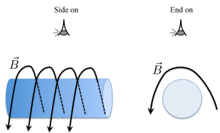
Figure 1: Wrapping of magnetic fields lines around a cylindrical filamentary structure (blue circle), as seen by the observer. This concept could provide an explanation for the observations seen in Orion-A, interacting with the Orion-Eridanus superbubble. The magnetic field line is represented as the curved black line.

We refer to this morphology, regardless of how it is formed, as a bow morphology. This general morphology has been recently investigated in some theoretical studies (Gómez et al. 2018; Inoue et al. 2018; Reissl et al. 2018), as well as observational studies (Liu et al. 2018), and has been also referred to as a U-shape or a pinched field.

Understanding the overall 3D magnetic field morphology, and consequently identifying which of these proposed magnetic configurations are responsible for the observed magnetic field reversals, can potentially help us answer questions pertaining to the role of magnetic fields in star formation. For example, helical fields can allow for more mass accumulation in the filamentary structure by stabilizing the cloud against self gravity (Buckle et al. 2012). Additionally, since the magnetic fields must form closed loops (zero-divergence), determining the 3D magnetic field morphology in and around these filaments can provide information regarding the influence that the surrounding environment has on the formation and evolution of filamentary structure.

In this paper we investigate the large-scale 3D magnetic field in Orion-A (the entire southern complex). For this purpose we use PXXXV dust polarization data and the TPBK18 B_∥ results. We discuss each of these datasets in Sec. 2 and describe our methodology to couple these two magnetic fields results in Sec. 3. Finally, we discuss our results and interpretation. The goals of TPBK18 and this paper are to provide techniques to obtain the large-scale structure of magnetic fields around star forming MCs. The broad-perspective intent is to show what can be done with the existing data, as well as to set the stage for future, higher sensitivity RM catalogs, which will be obtained by next generation surveys and telescopes.

2 Observations

Below we discuss the data we use for the line-of-sight and plane-of-sky components of the magnetic field in our study.

2.1 Line-of-sight magnetic field component

For the parallel component of the magnetic field (B_∥), we use the directions and magnitudes found in TPBK18. They calculate B_∥ using Taylor et al. (2009) rotation measure (RM) catalog, in combination with an electron column density estimated for each RM source from a chemical evolution code and Kainulainen et al. (2009) extinction maps. Additionally, they find B_∥ reversal across two regions of California and Orion-A molecular clouds. TPBK18 explains in detail how to find the B_∥ strengths and their uncertainty values. These uncertainties are calculated for each data point separately, and are due to the uncertainty propagation of all the required variables (input parameters) in determination of B_∥ strength.

In this paper, we consider only the magnetic field around Orion-A and use the data points that provide a solid direction for B_∥ (either towards or away from us). Consequently, if a B_∥ value has an uncertainty bigger than the value of B_∥ itself, we do not consider that data point in our analysis. That is, we use the B values with uncertainties $<$ 100% so that the direction of the field is well determined. For example, point 13 with $\text{B}_{\parallel}=-23\pm 38\,\mu$G (an uncertainty $>$ 100%) changes direction within its uncertainty range. We do not consider this point in our analysis, since its direction is highly uncertain. Fig. 2 shows all the data points determined in TPBK18. Points 3, 4, 6, 7, 8, 12, 15, 17, 18, 19, 29, 31, 32, and 34 in this figure have errors less than 100%. Points 4, 6, 12, 15, 17, 18, and 29, are considered in this study, since these are relatively close to the filament (filamentary structure) and are within the main axis length of the filament (see Sec. 3.1). In other words, these are the points with nearby B_⟂.

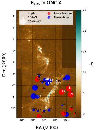
Figure 2: B_∥ in Orion-A. Blue (red) circles show magnetic fields toward (away from) us. The size of the circles indicate the magnitude of magnetic field. Sources numbered in bold white indicate the sources used for this study. Points 3, 4, 6, 7, 8, 12, 15, 17, 18, 19, 29, 31, 32, and 34 in this figure have errors less than 100%. Points 4, 6, 12, 15, 17, 18, and 29 are considered in this study.

2.2 Plane-of-sky magnetic field component

For the plane-of-sky component (B_⟂), we use the PXXXV determination of the magnetic field orientation as projected on the plane of the sky. As explained in PXXXV, we find the magnetic field lines from the thermal emission of interstellar dust observed by Planck at 353 GHz taken at an original resolution of $4^{\prime}.8$ and then smoothed with a $15^{\prime}$ FWHM Gaussian beam to guarantee signal-to-noise ratio of at least 3.

To find the average B_⟂ value in the Orion-A region we use the Planck dust polarization data along with the method of Davis-Chandrasekhar-Fermi (DCF) plus the structure function (DCF+SF) described by Hildebrand et al. (2009). To obtain the DCF components, we use the Planck 353 GHz data for the angle dispersion and CO observations for the density and line-of-sight velocity dispersion. The value we obtain is $180\pm 90\mu$G. This is a refined value tailored for Orion-A only, compared to what is mentioned in Table D.1 in PXXXV, which is for the entire Orion complex. Similar to B_∥, the B_⟂ uncertainty is as the result of uncertainty propagation of the input parameters (density and velocity dispersion) into determination of B_⟂. Even though these values do not represent B_⟂ magnitude for each data point of TPBK18 Orion-A map, where there is CO emission, the B_⟂ orientation at each point is determined from the Stokes parameters at that point.

3 Methodology

To investigate the validity of possible magnetic field morphologies, we model the different proposed configurations and compare the results of averaged magnetic fields along the LOS to those of observations.

3.1 Integrating the observations with models

In order to compare the modeled values with the observations, we need to find a B_⟂ value and orientation that can be associated with the B_∥ at each point from TPBK18. We do this by finding the closest PXXXV B_⟂ to the B_∥ points. If no B_⟂ value exists within $15^{\prime}$ (the size of the smoothed Planck polarization beam) of the B_∥ point, we discard that B_∥ point from our analysis. This also means that the B_∥ data point is too far from the filament (points 3, 8, 19 in Fig. 2). Points 31, 32, 34 and 7 are also too far away from the filament axis. Therefore, we carry out this study with points numbered 4, 6, 12, 15, 17, 18, and 29, as indicated by the white numbers in Fig. 2.

After finding the closest B_⟂ point to our B_∥ point, we find the orientation of B_⟂ by determining its polarization angle using:

$$\psi=\frac{1}{2}\arctan(-U,Q),$$ (1)

where $\psi$ is the polarization angle in the IAU convention, and U and Q are the Stokes parameters obtained from Planck observations of dust thermal radiation. We add a $\pi/2$ to $\psi$ to account for the fact that the magnetic field orientation ($\phi$) is orthogonal to the polarization angle. These angles are initially found with respect to the Galactic coordinate. To analyze the 3D geometry of the magnetic field with respect to the filament itself, we convert (rotate) these angles to the frame of reference of the filament itself.

We set the filament frame of reference such that the x-axis is radial to the filament and in the plane of the sky (i.e., the short axis of the filament in the plane of the sky from east to west), y-axis is parallel to the long axis of the filament in the plane of the sky, and z-axis is radial, towards the observer, as illustrated in Fig. 3. We can then write the magnetic field vector at each point in this frame of reference as ${\bf B}=(B_{x},B_{y},B_{z})$. Compared to the Galactic system, this new frame of reference is rotated by $\xi$, where $\xi$ is the angle the filament’s minor axis makes with decreasing Galactic longitude axis, i.e., the orientation of the x-axis of the filament with respect to East-West direction of the map measured in a clockwise direction.

In this system, $|B_{x}|=|B_{Planck}\sin(\xi+\phi)|$ and $|B_{y}|=|B_{Planck}\cos(\xi+\phi)|$, where $\phi$ is the magnetic angle in the plane of the sky and $B_{Planck}=180\pm 90\,\mu$G. The equations are cast as absolute values because we do not yet have any information regarding the positive/negative signs of $B_{x}$ and $B_{y}$ that provide the direction of B_⟂. While the orientation of B_⟂can be identified from the Stokes parameters, the actual direction (+ or $-$ along that orientation) cannot be determined. $B_{z}=$ B_∥ and does include the positive and negative signs of B_∥.

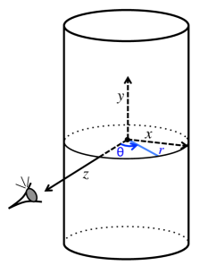
Figure 3: Geometry and coordinates for a filament. The x-axis is radial to the filament, and in the plane of the sky, y-axis is parallel to the long axis of the filament, and z-axis is radial, towards the observer.

Fig. 4 shows the resultant magnetic fields in the Cartesian frame illustrated in Fig. 3. In this figure, we take the ratio of the observed magnetic field components (i.e., $B_{x}$, $B_{y}$, $B_{z}$) to the total estimated observed magnetic field strength ($B_{total}=\sqrt{B_{x}^{2}+B_{y}^{2}+B_{z}^{2}}$). Considering the ratios helps us reduce the number of free parameters in the models. To distinguish between morphologies, we compare these observed magnetic field strengths to those predicted by our three models as described in sections below.

3.2 Modeling a toroidal and a helical 3D magnetic field

We model a filament with a simple toroidal or a helical magnetic field using the following set of equations:

$$B_{x}= \frac{B_{0}\text{R}\cos(\theta)}{r^{\alpha}}=\frac{B_{0}\text{R}z}{(x^{2}+z^{2})^{\frac{\alpha+1}{2}}},$$ (2)

$$B_{y}= \frac{B_{1}\text{R}}{r^{\alpha}}=\frac{B_{1}\text{R}}{(x^{2}+z^{2})^{\frac{\alpha}{2}}},$$

$$B_{z}= \frac{-B_{0}\text{R}\sin(\theta)}{r^{\alpha}}=\frac{-B_{0}\text{R}x}{(x^{2}+z^{2})^{\frac{\alpha+1}{2}}},$$

where the x, y, and z directions follow the convention set in Sec. 3.1 and Fig. 3. R is a scaling factor with units of [length]^α and $r=\sqrt{x^{2}+z^{2}}$ - the radial distance from the filament mid-plane in the X-Z plane (i.e., perpendicular to the long axis). $B_{0}$ and $B_{1}$ carry information about the strength of the toroidal and poloidal components of magnetic field respectively. The parameter $\alpha$ reflects the rate at which the magnetic field strength decreases with distance from the filament.

To have a purely toroidal magnetic field, or a helix with a small pitch angle, $B_{1}$ needs to be either zero or very small compared to $B_{0}$. In these equations, $\frac{x}{(x^{2}+z^{2})^{1/2}}$ and $\frac{z}{(x^{2}+z^{2})^{1/2}}$ replace $\sin\theta$ and $\cos\theta$.

Since a helical field threading a filament must be caused/produced by the filament itself, we assume its strength drops with distance from the filament’s main axis. The scaling factor R, therefore, arises from the relation between the strength of the magnetic field and its distance from the filament. This ensures that the units of both sides of these equations are identical (i.e., units of magnetic field strength).

To understand the rationale behind the magnetic strength decreasing with 1/r^α, we consider the following: the relation between the magnetic field and MC gas density; the observed density profile for the Orion-A filament; the necessity to keep the magnetic field divergence free.

The relationship between the magnetic field strength and the gas density has been investigated both theoretically and observationally. Theoretically, Tritsis et al. (2015) find that $B(\rho)\propto\rho^{1/2}$ is preferred, where $B(\rho)$ is the magnetic field as a function of the mass volume density and $\rho$ is the mass volume density. Observationally, Crutcher et al. (2010) propose a ratio of $B(\rho)\propto\rho^{2/3}$ when the magnetic energy is small compared to the effects of gravity. In our models, we consider both $B(\rho)\propto\rho^{1/2}$ and $B(\rho)\propto\rho^{2/3}$.

The density profile of the Orion-A filament has also been studied both observationally and theoretically and is proposed to have a Plummer-like form (e.g. Salji et al. 2015). The standard Plummer profile is described by:

$$\rho(r)=\frac{\rho_{c}}{\big{[}1+(r/r_{flat})^{2}\big{]}^{p/2}},$$ (3)

where $\rho_{c}$ is the central density of the filament, $r$ is the distance (radius) from the filament axis, and $r_{flat}$ is the characteristic radius defining the central region, where the density profile flattens. The exponent $p$ is observationally determined and sets the density drop-off rate. However, we use the more recently defined density profile suggested by Stutz & Gould (2016, See their equation 5), where they suggest that $\rho(r)\propto r^{-13/8}$. This density profile not only fits the observations, it also keeps our magnetic field divergence-free (i.e., $\frac{\partial B_{x}}{\partial x}+\frac{\partial B_{y}}{\partial y}+\frac{\partial B_{z}}{\partial z}=0$ in Equation 2). We extend this density profile to the larger Orion-A filamentary structure. Combining B$(\rho)$ with $\rho(r)$, we obtain a relation for B$(r)$ in which the magnetic field strength decreases as 1/r^α, where $\alpha$ can be either 13/16 or 13/12 depending on whether we use the Tritsis et al. (2015) or the Crutcher et al. (2010) relations.

3.3 Modeling a bow magnetic field morphology

The simplest divergence-free magnetic field relation one can use to describe a bow morphology is:

$$B_{x}= B_{1},$$ (4)

$$B_{y}= B_{2},$$

$$B_{z}= B_{0}\frac{x}{\text{R}^{\prime}},$$

where $B_{0}$, $B_{1}$, and $B_{2}$ are free parameters with positive values which provide the strength of magnetic field. R^′ is a free parameter with the unit of length to ensure that the relation for the z-component of magnetic field in equation 4 at both sides have the same units (see Sec. 4.3 for a range of values explored for these free parameters). $B_{x}$ and $B_{y}$ remain constant and in the direction of the ambient magnetic field, whereas $B_{z}$ varies with x. Since the value of the x-coordinate varies from positive to negative across the filament, this implies that $B_{z}$ reverses direction from one side of the filament to the other.

It is important to note that these equations represent single magnetic field lines. If we follow one field line as it wraps around a filament, we will see that the z-component (towards the observer) of the field is zero directly in front of, and behind, the filament. As we increase the radial distance from the filament (x-direction), the z-component will become larger. Thus, this relation of $B_{z}$ with $x$ represents the wrapping of the field lines around the filament, as well as the reversal.

Based on the model proposed by Heiles (1997), we assume that in the bow morphology the magnetic field components $(B_{x},B_{y},B_{z})$ represent field lines that do not penetrate the dense filament but, instead, represent the ambient magnetic field. Since they are ambient field lines, we do not expect a change of B-field strength as a function of distance from the filament’s long-axis. Therefore, we make the following assumptions: in the above set of equations for the bow model, the overall magnetic field strength does not decrease with distance; $B_{1}$ = $B_{2}$ represents the ambient magnetic field. Thus, we only explore different ratios of $B_{0}$ and $B_{1}$ (see Sec. 5).

If we forgo the $\nabla\cdot\mathbf{B}=0$ requirement, we can use the equations provided by Reissl et al. (2018), which model the bow morphology in a slightly different manner:

$$B_{x}= \frac{B_{0}(x,z)}{1+U^{2}(x,z)},$$ (5)

$$B_{y}= \leavevmode\nobreak\ 0,$$

$$B_{z}= \frac{B_{0}(x,z)U(x,z)}{1+U^{2}(x,z)},$$

with

$$U(x,z)=-5x(2-z)^{2}\leavevmode\nobreak\ e^{-8x^{2}},$$ (6)

$$B_{0}(x,z)=\frac{B_{0}}{(1+(r/r_{flat})^{2})^{-0.6\beta}}; r=\sqrt{x^{2}+z^{2}}.$$

$r_{flat}$ is the characteristic radius of the Plummer-like density profile (i.e., where the profile becomes flat close to the center of the filament). The parameter $\beta$ controls the slope of the density drop-off in the outer regions. Reissl et al. (2018) use $\beta$ = 1.6, which is the average value of $\beta$ from the Arzoumanian et al. (2011) density profile. $B_{0}$ controls the total strength of the magnetic field.

3.4 Comparing observed 3D magnetic field strengths with models

Since, along any given LOS we see a superposition of many different field lines, the observed magnetic field components $(B_{x},B_{y},B_{z})$ are averages over the LOS. To account for this in our models, we find the average magnetic field components along the LOS for each x, y, and z component of the field using the following integral:

$$<B_{i}>(x/\text{L})=\frac{\int^{+\frac{\text{L}}{2}}_{-\frac{\text{L}}{2}}B_{i}(x,z)dz}{\text{L}},$$ (7)

where L is the integration length along the LOS and $i$ indicates $x$, $y$, or $z$ components. Therefore, $<B_{i}>(x/L)$ is the average value of the $x$, $y$, or $z$ component of the magnetic field at a radial distance of $x$ from the filament long axis (the y-axis), and averaged over the line-of-sight distance of L. $B_{i}(x,z)$ is the magnetic field components from each models in equations 2, 4, and LABEL:Reissl. This calculation is performed for each of the models (toroidal/helical/bow) separately. Thus, equation 7 provides $<B_{x}>$, $<B_{y}>$, and $<B_{z}>$ as a function of $x$ (perpendicular distance to the filament axis) and L (integration path). We explore these averages as a function of $x$/L to avoid the need to convert $x$ and L to real distances and reduce the number of free parameters in the analysis. We set this integration distance (L) to be half of the distance of the point 17 from the filament axis, because we assume this distance represents the MC’s thickness along the LOS. One should note that finding the observed B_∥ values do not require the actual integration distance, since TPBK18 use the column density values in instead of the volume densities. Information about the line-of-sight integration distance is already embedded in the column densities.

To compare the models with the observed values, we determine the perpendicular distance (x) of each of our selected points in Fig. 2 from the filament axis. Additionally, we find the ratio of each x, y, and z component to the total (averaged along the LOS) magnetic field - both in the models and in the data, i.e., $(\frac{<B_{x}>}{<B_{total}>},\frac{<B_{y}>}{<B_{total>}},\frac{<B_{z}>}{<B_{total}>})$, where $B_{total}=\sqrt{<B_{x}>^{2}+<B_{y}>^{2}+<B_{z}>^{2}}$. These represent the ratios that should be observed ideally without experimental uncertainties and systematic observing biases. We then compare the above-mentioned ratios between the observed and modeled magnetic field components in order to determine which model is most consistent with the observed data. We perform this analysis in Sec. 4.

To compare the data with the models we employ a $\chi^{2}$ approach, using the following relation for each component of the magnetic field.

$$\chi^{2}_{i}=\sum_{j=1}^{N}\frac{\bigg{(}\text{observed }\frac{<B_{i}>}{<B_{tot}>}-\text{modeled}\frac{<B_{i}>}{{<B_{tot}>}}\bigg{)}^{2}_{j}}{\delta^{2}_{j}},$$ (8)

$$\chi^{2}_{tot}=\chi^{2}_{x}+\chi^{2}_{y}+\chi^{2}_{z},$$

where $i$ represents the $x$, $y$, or $z$ component of the magnetic field. N is the number of observational points in the study (in this paper $N=7$), and $\chi^{2}_{tot}$ is the total $\chi^{2}$. “Observed $\frac{<B_{i}>}{<B_{tot}>}$” is the observed ratio of each component of magnetic field to the total magnetic field as plotted in Fig. 4. “Modeled $\frac{<B_{i}>}{<B_{tot}>}$” is the LOS average of each model as explained in Sec. 3.4. $\delta$ represents the uncertainties of the magnetic field strengths determined in B_∥ and B_⟂ combined together. This $\delta$ is the unit-less relational uncertainty for the ratios as follows:

$$\delta=\sqrt{(\frac{\delta B_{||}}{B_{||}})^{2}+(\frac{\delta B_{\perp}}{B_{\perp}})^{2}},$$ (9)

where $\delta B_{||}$ is the uncertainty of B_∥ and $\delta B_{\perp}$ is the uncertainty of B_⟂. For example, for point number 29 in Fig. 2, with $\text{B}_{\parallel}=-418\pm 308\,\mu$G and $\text{B}_{\perp}=180\pm 90\,\mu$G, $\delta$ is calculated as follows:

$$\delta=\sqrt{(\frac{308}{418})^{2}+(\frac{90}{180})^{2}}=0.89.$$ (10)

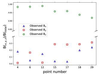
Figure 4: Observed $B_{x}$, $B_{y}$, and $B_{z}$ using the frame system depicted in Fig. 3 as well as B_⟂ and B_∥ values obtained by PXXXV and TPBK18  respectively. The y-axis shows the ratio of each component of magnetic field to the total value and the x-axis refers to the numbered data points labeled in Fig. 2.

4 Results of modeling

Fig. 4 demonstrates the ratio of the observed magnetic field components (i.e., $B_{x}$, $B_{y}$, $B_{z}$) to the total estimated observed magnetic field strength ($B_{total}=\sqrt{B_{x}^{2}+B_{y}^{2}+B_{z}^{2}}$), in the filament’s Cartesian frame shown in Fig. 3. To determine which of our three models best fits the data, we compare the predicted magnetic field strengths for each of the models to these observed values.

4.1 The toroidal morphology

We investigate the Toroidal model using equation 2 and setting $B_{1}=0$ (i.e., a helix with zero pitch angle). By considering the ratios of each component of the magnetic field to the total averaged magnetic field value, the free parameters R and $B_{0}$ cancel out and do not contribute to the final results.

The top row of Fig. 5 shows the results of the toroidal model for the two different assumptions of the relationship between magnetic field strength and density: alpha = 13/16 (left) and 13/12 (right). The symbols represent the observed values, and the lines depict the model results as described in Sec. 3.4. The blue, red, and green colors illustrate the x, y, and z components, respectively. Both alpha values produce identical model results, which indicates that the decrease of magnetic field strength with distance does not play a noticeable role.

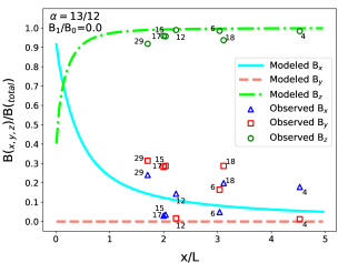
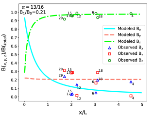
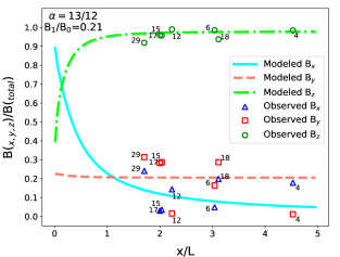
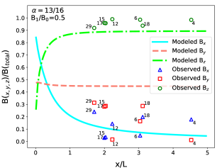
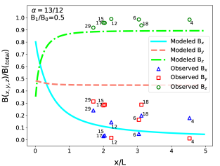
Figure 5: Best fits for modeled toroidal and helical fields. Colored lines represent the modeled x,y, and z components of the magnetic field. The colored symbols represent the x, y, and z components of the observed magnetic field. On the x-axis, X is the perpendicular distance from the filament’s long axis, and L is the LOS integration distance. The two $\alpha$ values are the parameters explained in Sec. 3.2. The different $B_{1}$/$B_{0}$ ratios arise from equation 2 and set the level of helicity, with $B_{1}$/$B_{0}=0$ indicating a purely toroidal field.

The top row of Fig. 5 suggests that while the toroidal model seems to provide a good match to the z-component of the magnetic field, the modeled x- and y-components do not. The corresponding $\chi^{2}$ value for each component are: $\chi^{2}_{x}=0.109$, $\chi^{2}_{y}=0.778$, $\chi^{2}_{z}=0.020$, and $\chi^{2}_{tot}=0.908$ for both $\alpha$ = 13/16 and 13/12.

4.2 The helical morphology

The pitch angle of a helix can be parameterised by the ratio of $B_{1}$/$B_{0}$ in equation 2. Increasing this ratio increases the pitch angle. After taking the LOS averages (see Sec. 3.4) $B_{1}$ and $B_{0}$ do not cancel out but instead remain as free parameters. Thus, to study a helical model, we use equation 2 and vary the ratio of $B_{1}$/$B_{0}$, from 0.0 to 1.49 in step sizes of 0.01. For each value of $B_{1}$/$B_{0}$ we calculate the corresponding $\chi^{2}$ value. The minimum $\chi^{2}$ is calculated as the sum of the $\chi^{2}$ for all the components (i.e., $\chi^{2}_{tot}$). We also pay particular attention to the y-component, since it sets the toroidal model apart from the helical one. The lowest $\chi^{2}$ occurs for $B_{1}$/$B_{0}=0.21$ (both with $\alpha$ = 13/16 and 13/12), with $\chi^{2}_{x}=0.109$, $\chi^{2}_{y}=0.193$, $\chi^{2}_{z}=0.008$, $\chi^{2}_{tot}=0.310$. The two bottom rows of Fig. 5 represent the modeled helical morphology for $\alpha$ = 13/16 (left) and 13/12 (right). The middle, and the bottom rows show $B_{1}$/$B_{0}$ value of 0.21 (the best $\chi^{2}$ fit result) and 0.5, respectively.

4.3 The bow morphology

To model the bow magnetic morphology, we use equation 4 and find the ratio of each magnetic field component to the total magnetic field (as explained in Sec. 3.4). Since the free parameters $B_{1}$, $B_{0}$, and R^′ do not cancel out, we explore different values of $B_{0}$/$B_{1}$ and R^′. To explore these free parameters, we first pick arbitrary values that result in a best visual fit with the data. For R^′, this initial value is equal to the integration distance, i.e., half of the perpendicular distance of point 17 from the filament axis. We then explore the influence of larger and smaller values of these free parameters in a quantitative manner. In addition, in equation 4, we assume $B_{2}$ = $B_{1}$, so that the x and y components of the magnetic field are equal, and then explore a range to find the lowest $\chi^{2}$ results. Since the observed B_∥ values are higher than the Planck B_⟂ average strength, we start from $B_{1}$/$B_{0}=0.5$ and calculate the $\chi^{2}$ for various R^′ values up to $B_{1}$/$B_{0}=15$, with step-size of 0.5. We take this range of parameters because we find that they fit the data better visually. In this range of $B_{1}$/$B_{0}$, we explore the R^′ values from 0.3 of the integration distance (0.3L) up to 3.2L, with step-size of 0.1. Fig. 6 shows the results for this bow model for two sets of free parameters, the left panel represents a set of parameters that produce the smallest $\chi^{2}$ result. The best-fit model is for $B_{0}$/$B_{1}=3.5$ and R${}^{\prime}=1.3$L with $\chi^{2}_{x}=0.158$, $\chi^{2}_{y}=0.181$, $\chi^{2}_{z}=0.007$, $\chi^{2}_{tot}=0.346$.

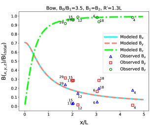
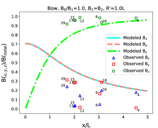
Figure 6: Bow magnetic morphology from equation 4. The magnetic fields are averaged along the LOS. Colored lines represent the modeled x,y, and z components of the magnetic field. The colored symbols represent the x, y, and z components of the observed magnetic field. On the x-axis, X is the perpendicular distance from the filament’s long axis, and L is the LOS integration distance. The parameters show different $B_{1}$/$B_{0}$ ratios from equation 4. Left panel shows the best fit for equation 4.

To explore the bow model further, we consider equation LABEL:Reissl, as described in Sec. 3.3. For this purpose we modify the equations slightly to represent a more general form and to be compatible with our filament setup (i.e., to account for the reversal in the scales observed in TPBK18 and to make sure the units in the right and left hand sides of equation LABEL:Reissl are the same [$\mu$G]). We set U(x,z) in equation 6 as:

$$U(x,z)=b_{R}x(c_{R}-z)^{2}\exp(a_{R}x^{2}),$$ (11)

where a_R, b_R, and c_R are free parameters. These parameters help the observed and modeled results to be close to each other visually.

To explore a range of free parameters, we set a_R, b_R, and c_R in form of $\frac{-8}{(a\text{L})^{2}}$, $\frac{-5}{(b\text{L})^{2}}$, and c${}_{R}=c$L, where a, b, and c are scalar values. In order to reduce the number of free parameters, we take the parameters as a function of L. These forms result in a unit of $\mu$G in equation LABEL:Reissl. We subsequently explore different a, b, and c values where $5\leq a\leq 17$ with step-sizes of 0.5, $0.2\leq b\leq 3$ with step-size of 0.2, and $1\leq c\leq 15$ with step-sizes of 1. Fig. 7 shows the results for [a${}_{R}=\frac{-8}{(9.5\text{L})^{2}}$, b${}_{R}=\frac{-5}{(2.2\text{L})^{2}}$, and c${}_{R}=10$L] and for [a${}_{R}=\frac{-8}{(8\text{L})^{2}}$, b${}_{R}=\frac{-5}{\text{L}^{2}}$, and c${}_{R}=3$L]. We notice that different values of r_flat do not generate any noticeable differences in final results, since we consider the ratios.

Since the B_y component is zero in this version of bow model, $\chi_{y}^{2}$ is constant and determined to be 0.778. This is lower than that of the Toroidal model, but higher than those of both the helical and bow models from equation 4. We find that a few sets of parameters with $a=9.5$ result in the lowest $\chi^{2}$with c in a range of 9 to 13 and b in range of 2.0 to 2.8. For example a = 9.5, b = 2.2, and c = 10 (i.e., a${}_{R}=\frac{-8}{(9.5\text{L})^{2}}$, b${}_{R}=\frac{-5}{(2.2\text{L})^{2}}$, and c${}_{R}=10$L) or a = 9.5, b = 2.4, and c = 11 produce $\chi^{2}$ result of $\chi^{2}_{x}=0.073$, $\chi^{2}_{y}=0.778$, $\chi^{2}_{z}=0.021$, $\chi^{2}_{tot}=0.872$. Given the small step-sizes having a range for the smallest $\chi^{2}$ is expected. For this bow model, we pick the set of parameter that when we consider more significant digits of $\chi^{2}$, they result in the smallest $\chi^{2}$. That is with a${}_{R}=\frac{-8}{(9.5\text{L})^{2}}$, b${}_{R}=\frac{-5}{(2.2\text{L})^{2}}$, and c${}_{R}=10$L.

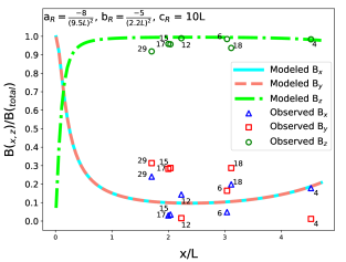
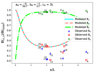
Figure 7: Bow magnetic morphology from equation LABEL:Reissl. The magnetic fields are averaged along the LOS. Colored lines represent the modeled x,y, and z components of the magnetic field. The colored symbols represent the x, y, and z components of the observed magnetic field. On the x-axis, X is the perpendicular distance from the filament’s long axis, and L is the LOS integration distance. Left panel shows the best fit for equation LABEL:Reissl.

Finally, we should note that in equations LABEL:Reissl and 6, the density is that of a Plummer-like profile to relate magnetic strength to r in $B_{0}(x,z)$. An alternative approach is to use the earlier proposed relation between the magnetic strength and r (see Sec. 3.2) of

$$B_{0}(x,z)=\frac{B_{0}}{(x^{2}+z^{2})^{\frac{-\alpha}{2}}}.$$ (12)

However, even with this density profile, equation LABEL:Reissl for this bow model is not divergence-free. We find that using the two different density profile does not provide noticeably different results.

Finally, we note that these results are based on magnetic field values that have large uncertainties and possibly have systematic biases. To alleviate the dependency of our interpretation of the 3D magnetic field morphology on sole values of B_⟂ and B_∥  we carry out a Monte-Carlo analysis in Sec. 5.

5 Discussion

In this section we explore the results further and propose the most likely magnetic field morphology for Orion-A. We then consider effects that may have biased our results.

5.1 A Monte-Carlo analysis

PXXXV provide a magnetic field value (B_⟂) that is averaged over the entire Orion-A region, whereas TPBK18 provide the B_∥ field values for very specific points with observed RMs. Thus, applying this single value of B_⟂ to every RM position comes with significant uncertainties. In addition, the values of B_∥ from TPBK18 come with their own, inherently large, uncertainties. To account for these uncertainties, we perform a Monte-Carlo error analysis to compare the models with the observed magnetic field components. In this approach, we randomly alter the B_∥ and B_⟂ strengths of each single data point separately within their uncertainty ranges and, for each iteration, compare the models with the data. More specifically, we

1. Randomly changed B_∥ for each data point within its uncertainty range (from TPBK18).

2. Randomly changed the strength of Planck magnetic field (B_⟂) for each data point separately within its uncertainty range ($\pm 90\,\mu$G).

3. Calculated the “new” $B_{x}$, $B_{y}$, and $B_{z}$ values, using the “new” B_⟂ and B_∥ values for each data point.

4. Found the differences ($\varsigma$) between the “new” $B_{x}$, $B_{y}$, and $B_{z}$ values and the best toroidal/helical/bow models found in Sec.4 using the equations:

   $$\varsigma_{x}=\sum_{i=1}^{N}(|B_{x,\text{ modeled}}|-|B_{x,\text{ observed}}|)_{i}^{2},$$ (13)

   $$\varsigma_{y}=\sum_{i=1}^{N}(|B_{y,\text{ modeled}}|-|B_{y,\text{ observed}}|)_{i}^{2},$$

   $$\varsigma_{z}=\sum_{i=1}^{N}(|B_{z,\text{ modeled}}|-|B_{z,\text{ observed}}|)_{i}^{2},$$

   $$\varsigma_{\text{total}}=\varsigma_{x}+\varsigma_{y}+\varsigma_{z},$$

   where N is the number of data points (N = 7).

5. Found which of our best toroidal/helical/bow models has the lowest $\varsigma_{\text{total}}$ value when compared against the “new” (i.e., randomly altered) data.

This Monte-Carlo analysis was done 50,000 times. Our bow model had the smallest difference (i.e., the bow model best fits the data) 34,177 times. The helical model had the smallest difference 15,823 times. In no cases did the toroidal model have the smallest difference.

5.2 Systematic biases

Since B_⟂ and B_∥ are derived in completely different ways (using Faraday rotation for B_∥ and dust polarization for B_⟂), we probe the effects of potential systematic biases between the results of the two methods. Additionally, we should note that our values of B_∥ are generally larger than the B_⟂ value and the B_⟂ value is an average for the region. Therefore, our B_⟂ could be systematically lower than B_∥. To investigate potential systematic biases, we explored a range of factors multiplied by our B_∥ and B_⟂ separately, and repeated a process similar to that presented in Sec. 5.1. In more details, we

1. Multiplied all of our B_∥ values by a randomly generated factor between 0.5 and 5 (same factor for all of the B_∥ values).

2. Multiplied the B_⟂ value by a randomly generated factor between 1 and 5.

3. Calculated the “new” $B_{x}$, $B_{y}$, and $B_{z}$ values, using the “new” B_⟂ and B_∥ values for each data point.

4. Using equation 13, found the differences ($\varsigma$) between the “new” $B_{x}$, $B_{y}$, and $B_{z}$ values and the best toroidal/helical/bow models found in Sec.4.

5. Found which of our best toroidal/helical/bow models has the lowest $\varsigma_{\text{total}}$ value when compared against the “new” data.

This analysis was done 50,000 times. Our bow model had the smallest difference (i.e., the bow model best fits the data) for 25002 times. The bow shape in form of equation 11 and the helical model had the smallest difference for 5195 and 19803 times, respectively. Therefore, considering this range of systematic biases, the bow model seems to be a better fit.

5.3 Selecting the best magnetic field morphology

To compare the toroidal and helical models we only need to compare the $\chi^{2}$ values of the two models with each other. This is because these two models are a single model with different parameters (one with $B_{1}$/$B_{0}=0$ and the other with $B_{1}$/$B_{0}=0.21$). Therefore, since $\chi^{2}_{tot}=$ 0.310 for the helical model and 0.908 for the toroidal model, we suggest a helical morphology fits the data better. Furthermore, since it is the y-component that sets the toroidal and helical models apart, visually comparing the y-component in the top panel of Fig. 5 with the middle-left panel illustrates that a helical model (with $B_{1}$/$B_{0}=0.21$) is a better fit to the data. This is borne out in the mathematical analysis which shows that $\chi^{2}_{y}=$ 0.193 for the helical model and 0.778 for the toroidal model.

To compare the bow morphology to the helical/toroidal one, we first compare the left panel of Fig. 6 and the left panel of Fig. 7 with the helical and toroidal models in Fig. 5. From these figures it is easy to see that the bow models fit the data better than a toroidal model. However, it is difficult to see if either of the bow models fit the data better than the helical model. Thus, a more robust comparison is required.

Since the bow and toroidal/helical morphologies are represented by two very different models, one cannot simply compare their $\chi^{2}$ values. Thus, to compare the bow morphology to the toroidal/helical one, we compare their probability values (i.e., p-values). P-values allow one to compare different models by providing the probability for a statistically relevant model. The probability value provides the likelihood that a hypotheses (toroidal, helical, or bow) is true (Sivia & Skilling 2006). In statistical analysis, p-values are normally used to reject a null hypothesis. If we assume that they represent a Gaussian distribution, it is a measure to understand whether the result from the hypothesis is closer to the peak of the distribution or its tail. A model/hypothesis can be ruled out if the p-value is less than a threshold, typically 0.05.

To find the p-values, we need the $\chi^{2}$ values and the degrees of freedom (DOF) of the model. For the helical model we take one degree of freedom (i.e., $B_{1}$/$B_{0}$) for the first bow model we take two degrees of freedom (i.e., $B_{0}$/$B_{1}$, and R^′) for the second bow model we take three degrees of freedom (i.e., a_R, b_R, and c_R). Our best fit bow model ($\chi^{2}_{tot}$ =0.346 with two DOFs) has a p-value of 0.84. Our best helical model ($\chi^{2}_{tot}=0.310$ with one DOF) has a p-value of 0.58. Based on these p-values none of the models can be ruled out. We should note that the Reissl et al. (2018) bow model ($\chi^{2}_{tot}$ = 0.872 with three DOF) has a p-value of 0.83 - similar to that of our bow model.

Therefore, it is likely that the bow morphology is more probable than both the helical and toroidal. Additionally, the results of the Monte-Carlo analysis and our systematic bias investigation lend support to our suggestion that the bow model is, overall, the most likely fit to the observed magnetic fields in the Orion-A filament.

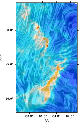
Figure 8: Column density and magnetic field toward the Orion region. The colors correspond to the dust opacity derived from the Planck observations. The drapery pattern corresponds to the orientation of the magnetic field projected on the plane of the sky and integrated along the line of sight, as inferred from the Planck 353-GHz observations. The yellow color between declination of about $-5^{\circ}$ and $-10^{\circ}$ show the Orion-A filamentary structure as illustrated in Fig. 2. The B_⟂ lines on one side of this filament are mostly perpendicular to the filament (representing a small pitch angle for a helical morphology) while, on the other side, they are more parallel to the filament.

Furthermore, as shown by the Planck results in Fig. 8, the B_⟂ lines on one side of the Orion-A filament are mostly perpendicular to the filament (representing a small pitch angle for a helical morphology) while, on the other side, they are more parallel to the filament. Therefore, if we assume a helical magnetic field morphology for the Orion-A region, we would have to consider completely different pitch angles for the two sides of the filament which is not sensible. Therefore, this simple visual analysis of the B_⟂ orientation also seems to suggest that a bow morphology is a more natural fit to the data.

5.4 Tilted models for Orion-A

Finally, we briefly explore the effects of 3D geometry on our results. Recent observations by Großschedl et al. (2018) show that the Orion-A filamentary structure is inclined along the LOS with respect to the observer. However, they show that different parts of this region have different inclination angles. The part of the Orion-A region that contains Orion KL has a close-to-zero tilt. In particular, the region that contains L1641-N in Orion-A, which is very close to 6 of the 7 data points taken in our analysis, has zero inclination in Fig. 3 of Großschedl et al. (2018). Due to this zero inclination at the region where our data points are accumulated, we suggest that we do not need to consider inclination of the Orion-A region along the line-of-sight for this study.

Consequently, the models of equations 2, 4, and LABEL:Reissl represent a filament that is assumed to be lying in the plane of the sky without being tilted away from, or towards, the observer. With future data sets, where the data points are accumulated all along the Orion-A region, considering a more complex 3D geometry incorporating the study of Großschedl et al. (2018), is required. In that case, if one considers a tilted filament, the equations representing the models will not change since the frame of reference is adjusted to the filament as illustrated in Fig. 3. However, when taking the average of each magnetic field component along the line-of-sight, one has to adjust $dz$ in equation 7, such that this $dz$ is the line-of-sight path length from the observer’s point of view and not in the filament’s reference frame.

6 Conclusions

We present 3D magnetic field modelling around the Orion-A molecular cloud using existing dust polarization observations, which provide the plane-of-sky magnetic field, combined with the line-of-sight magnetic fields obtained by the method presented in Tahani et al. (2018). We first construct models describing a toroidal, helical, and a bow-shape magnetic field morphology. While all three morphologies can explain the line-of-sight magnetic field reversal around Orion-A as observed by Tahani et al. (2018), we suggest that the bow morphology is the most natural magnetic field morphology for the Orion-A region.

This conclusion is based on the following arguments:

1. The bow model has the highest p-values.

2. Our bow model seems to be the most consistent model with the observational data and their uncertainty values in our Monte-Carlo analysis approach, as well as with our investigation of systematic biases.

3. Different B_⟂  angles on the eastern side of the filament compared to the western side suggests that the data cannot be properly modeled by a single helix with the same pitch angle on both sides of the filament.

The analysis in this paper utilises the best rotation measure data currently available in the entire Orion-A region. As such, it is limited to the number of available RM sources in the Taylor et al. (2009) catalog, as well as the sensitivity of those observations. This analysis is also limited by the fact that the Planck maps provide only one value for B_⟂ averaged across the entire region. Our results stress the need for more RM observations and higher-angular resolution dust polarization maps to further reconstruct the 3D magnetic field morphology.

Future RM catalogs from new generation surveys such as POSSUM and VLASS will allow for the detection of a higher number of B_∥ sources and with better sensitivity. Thus, these new catalogs will provide better-sampled maps of the large-scale B_∥ magnetic field with smaller errors. Combined with new and improved dust polarization maps (from instruments like APEX, ALMA, BLASTPOL2), future applications of the analyses presented in this work will allow us to map and model the 3D magnetic field geometry with better accuracy.