Abstract

In this paper we will show that one can summarize the major two particle reaction plane azimuthal correlations for Au + Au mid-central collisions at $\sqrt{s_{NN}}=$ 200 GeV by defining a 2D azimuthal space which is a summary of the event by event average.

1 Introduction to Three Particle and Reaction Plane Two Particle Azimuthal Correlations.

In this paper we are interested in four three particle azimuthal correlations. These correlations are defined by the four equations below

$$C_{112}=\langle cos(\phi_{1}+\phi_{2}-2\phi_{3})\rangle,$$ (1)

$$C_{123}=\langle cos(\phi_{1}+2\phi_{2}-3\phi_{3})\rangle,$$ (2)

$$C_{132}=\langle cos(\phi_{1}-3\phi_{2}+2\phi_{3})\rangle,$$ (3)

$$C_{143}=\langle cos(\phi_{1}-4\phi_{2}+3\phi_{3})\rangle,$$ (4)

where $\phi_{1}$, $\phi_{2}$, $\phi_{3}$ denote the azimuthal angles of the produced particle 1, produced particle 2 and produced particle 3.

For Au + Au mid-central collisions at $\sqrt{s_{NN}}=$ 200 GeV, the quadrupole flow from an impact angle defines the orientation Au + Au collision and defined the angle of $v_{2}$. This $v_{2}$ angle is charge independent only determined by geometry. If we choose $\phi_{3}$ to be charge independent and coming from particles which range over the whole event, we can replace $\phi_{3}$ with $\psi_{2}$ the quadrupole flow angle for the first and third equations. For each event there will also be a hexapole flow angle for $v_{3}$ which gives a $\psi_{3}$ which can be used in the second and fourth equations.

$$C_{112}=\langle cos(\phi_{1}+\phi_{2}-2\psi_{2})\rangle,$$ (5)

$$C_{123}=\langle cos(\phi_{1}+2\phi_{2}-3\psi_{3})\rangle,$$ (6)

$$C_{132}=\langle cos(\phi_{1}-3\phi_{2}+2\psi_{2})\rangle,$$ (7)

$$C_{143}=\langle cos(\phi_{1}-4\phi_{2}+3\psi_{3})\rangle,$$ (8)

For this paper we will choose $\psi_{2}$ to be zero. This requires that all events are rotated in azimuth such that $\psi_{2}$ becomes zero. In general the $\psi_{3}$ points in some other direction. With this choice of $\psi_{2}$, we show in Ref[1] that there is a mono jet effect with squeeze out flow of particles around the mono jet which gives a $\psi_{3}$ pointing in the $-90^{\circ}$ or -$\pi\over 2$ direction. This implies that the mono jet points in the $90^{\circ}$ or $\pi\over 2$ direction.

Also this paper will consider particles produced around central rapidity and concentrate on two particle azimuthal correlations(see above). There is an another two particle azimuthal correlation which does not depend on any axis

$$\delta=\langle cos(\phi_{1}-\phi_{2})\rangle.$$ (9)

There is a simple relationship between equation 5 and equation 9 since $\psi_{2}$ = 0..

$$C_{112}=\langle cos(\phi_{1}+\phi_{2})\rangle=\langle cos(\phi_{1})cos(\phi_{2})\rangle-\langle sin(\phi_{1})sin(\phi_{2})\rangle,$$ (10)

$$\delta=\langle cos(\phi_{1}-\phi_{2})\rangle=\langle cos(\phi_{1})cos(\phi_{2})\rangle+\langle sin(\phi_{1})sin(\phi_{2})\rangle.$$ (11)

Thus $\langle$ $cos(\phi_{1})$ $cos(\phi_{2})$ $\rangle$ and $\langle$ $sin(\phi_{1})$ $sin(\phi_{2})$ $\rangle$ are also values we calculate in this paper. .

Finally the quadrupole and the hexapole are global event objects while $\delta$ the two particle correlation is a more local effect. In the appendix we show that just the presents of $v_{2}$, $v_{3}$ and a $\delta$ can generate three particle correlation. In our analysis we are dealing with the Case II of the appendix which consider only particles produced around central rapidity and the results from Au + Au mid-central collisions at $\sqrt{s_{NN}}=$ 200 GeV are inconsistent with the appendix.

The paper is organized in the following manner:

Sec. 1 is the introduction to the two particle reaction plane azimuthal correlations for heavy ion Au + Au mid-central collisions. Sec. 2 the additions to Ref[1] same sign pairs correlation. Sec. 3 $\phi_{1}$ and $\phi_{2}$ azimuthal two particle plane. Sec. 4 the two particle correlation from the $\phi_{1}$ and $\phi_{2}$ azimuthal plane. Sec. 5 calculation of correlations using the distribution of the $\phi_{1}$ and $\phi_{2}$ azimuthal plane. Sec. 6 presents the summary and discussion.

2 Additions to Ref[1] Same Sign Pairs Correlation.

In this paper we where inspired by the squeeze out of particles around the mono jet of Ref[1] to establish an orientation of the hexapole flow axis with respect to the quadrupole flow axis. In the introduction we determined that $\langle$ $cos(\phi_{1})$ $cos(\phi_{2})$ $\rangle$ and $\langle$ $sin(\phi_{1})$ $sin(\phi_{2})$ $\rangle$ are very important correlations to be explored. Thus we see in Ref[1] when we compare to Ref[2] there is a systematic difference. In the flux tube model[3, 4] there is conservation of momentum between the flux tubes such that there is a negative correlation when one compares particles coming from tubes at different pseudo rapidity($\eta$). When we concentrate on like sign particle pairs this effect is much stronger than the model of Ref[1].

In Figure 1 we show the $\langle$ $cos(\phi_{1})$ $cos(\phi_{2})$ $\rangle$ and $\langle$ $sin(\phi_{1})$ $sin(\phi_{2})$ $\rangle$ for same sign pairs and opposite sign pairs as a function $\Delta\eta$($|\eta_{1}-\eta_{2}|$) of Ref[1]. This should be compared to FIG 8 of Ref[2]. For like sign particle pairs between a flux tube and other tubes there is a greater a negative correlation of momentum conservation at smaller $\Delta\eta$ than Ref[1] so we increase this negative correlation to become in agreement with Ref[2] see Figure 2. With the addition of this same negative correlation to the like sign particle pairs correlation for $\langle$ $cos(\phi_{1})$ $cos(\phi_{2})$ $\rangle$ and $\langle$ $sin(\phi_{1})$ $sin(\phi_{2})$ $\rangle$ we do not cause a change in the results of Ref[1]. This is because they depend on the difference between the two terms and thus subtract out.

Figure 1: An angular correlation $\langle cos(\phi_{1}(\eta_{1})+\phi_{2}(\eta_{2}))\rangle$ for like sign and unlike sign pairs is split up into in plane $\langle cos(\phi_{1}(\eta_{1}))cos(\phi_{2}(\eta_{2}))\rangle$ and out of plane $\langle sin(\phi_{1}(\eta_{1}))sin(\phi_{2}(\eta_{2}))\rangle$ parts. The in plane is the flux tubes while the out of plane is the CME(like sign) and the mono jet effect(both). The simulation is for mid-central Au-Au collision $\sqrt{s_{NN}}$ = 200.0 GeV

Figure 2: Like sign and unlike sign pairs as seen in Figure 1 is split up into in plane $\langle cos(\phi_{1}(\eta_{1}))cos(\phi_{2}(\eta_{2}))\rangle$ and out of plane $\langle sin(\phi_{1}(\eta_{1}))sin(\phi_{2}(\eta_{2}))\rangle$ parts. A negative correlation of momentum conservation is add to both in plane and out of plane like sign pairs only so it agrees with Ref[2]. The simulation is for mid-central Au-Au collision $\sqrt{s_{NN}}$ = 200.0 GeV

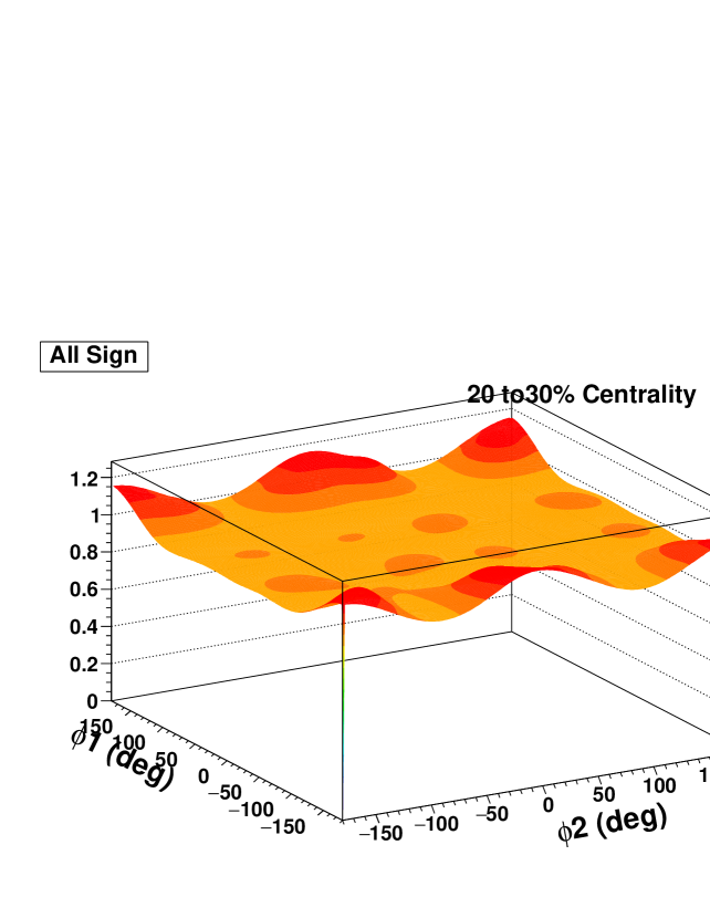
Figure 3: The reaction plane has two azimuthal angles $\phi_{1}$ and $\phi_{2}$ where geometry defined an $v_{2}$ axis to lie in the $0^{\circ}$ to $180^{\circ}$ axis. In Ref[1] the presence of out of plane mono jets then gives us a $v_{1}$ which we require to point along the $90^{\circ}$ axis. The squeeze out flow around the hot spot of mono jet causes the $v_{3}$ axis to point along the $-90^{\circ}$ axis. We show the distribution for all particle pairs.

3 $\phi_{1}$ and $\phi_{2}$ Azimuthal Two Particle Plane.

The main objective of this paper is to introduce the concept of summarizing the azimuthal two particle correlations with respect to the reaction plane for heavy ion Au + Au mid-central collisions, by using a $\phi_{1}$ and $\phi_{2}$ azimuthal two particle plane. For each mid-central collision we have a well defined $v_{2}$ axis given by geometry. We assign this well defined axis to lie in the $0^{\circ}$ to $180^{\circ}$ axis. In Ref[1] the presence of out of plane mono jets then gives us a $v_{1}$ which we require to point along the $90^{\circ}$ axis. The squeeze out flow around the hot spot of mono jet causes the $v_{3}$ axis to point along the $-90^{\circ}$ axis.

This paper contends that the event average of the azimuthal two particle angles $\phi_{1}$ and $\phi_{2}$ with respect to the reaction plane as defined above captures the azimuthal correlation structure of the Au + Au mid-central collisions. We use Ref[1] modified as pointed out in section 2 to generate a event average $\phi_{1}$ and $\phi_{2}$ plane distribution. In Figure 3 we show the event averaged $\phi_{1}$ and $\phi_{2}$ plane distribution for all particle pairs which we have generated from the above method.

In Figure 4 we show the event averaged $\phi_{1}$ and $\phi_{2}$ plane distribution for opposite charged particle pairs. Opposite charges are greatly influenced by the fragmentation of the charge neutral quark gluon plasma. We see an asymmetry in the $\phi_{1}$ and $\phi_{2}$ plane distribution, because once we choose one charge the distribution of the other charge is different due to fragmentation effects.

Finally in Figure 5 we show the event averaged $\phi_{1}$ and $\phi_{2}$ plane distribution for same charged particle pairs. The same charges must have a symmetry in the $\phi_{1}$ and $\phi_{2}$ plane, since we have Bose symmetry particle 1 and 2 are interchangeable.

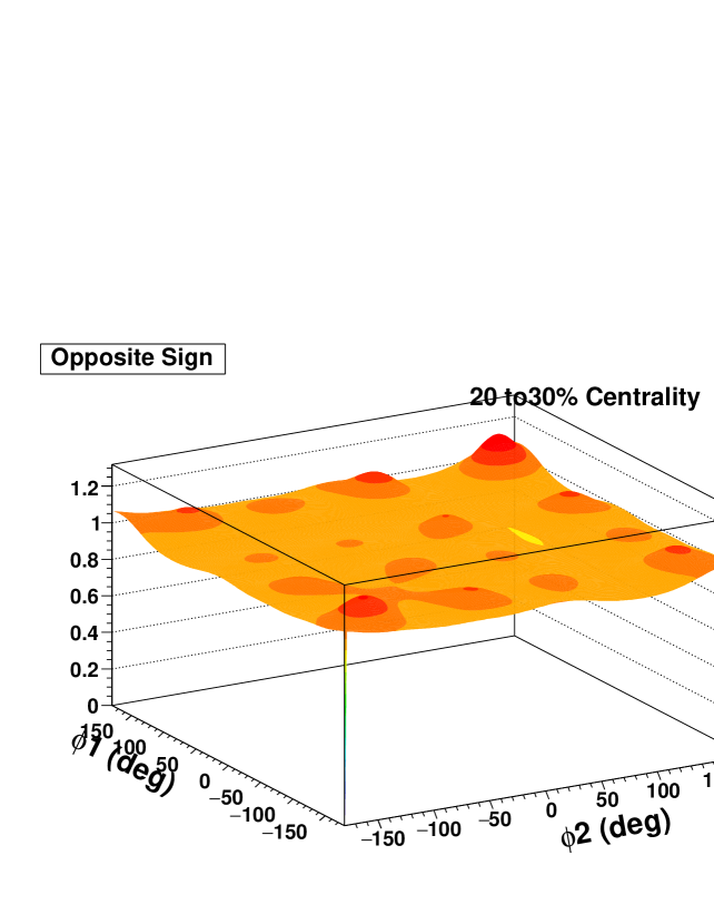
Figure 4: The reaction plane has two azimuthal angles $\phi_{1}$ and $\phi_{2}$ where geometry defined an $v_{2}$ axis to lie in the $0^{\circ}$ to $180^{\circ}$ axis. In Ref[1] the presence of out of plane mono jets then gives us a $v_{1}$ which we require to point along the $90^{\circ}$ axis. The squeeze out flow around the hot spot of mono jet causes the $v_{3}$ axis to point along the $-90^{\circ}$ axis. We show the distribution for unlike sign particle pairs.

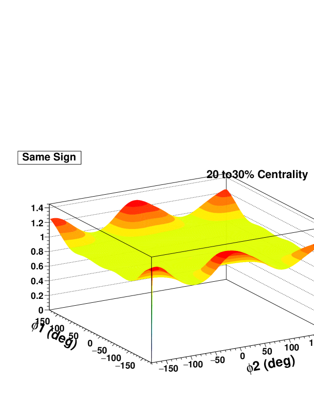
Figure 5: The reaction plane has two azimuthal angles $\phi_{1}$ and $\phi_{2}$ where geometry defined an $v_{2}$ axis to lie in the $0^{\circ}$ to $180^{\circ}$ axis. In Ref[1] the presence of out of plane mono jets then gives us a $v_{1}$ which we require to point along the $90^{\circ}$ axis. The squeeze out flow around the hot spot of mono jet causes the $v_{3}$ axis to point along the $-90^{\circ}$ axis. We show the distribution for like sign particle pairs.

Figure 6: The reaction plane has two azimuthal angles $\phi_{1}$ and $\phi_{2}$ where geometry defined an $v_{2}$ axis to lie in the $0^{\circ}$ to $180^{\circ}$ axis. In Ref[1] the presence of out of plane mono jets then gives us a $v_{1}$ which we require to point along the $90^{\circ}$ axis. The squeeze out flow around the hot spot of mono jet causes the $v_{3}$ axis to point along the $-90^{\circ}$ axis. The two particle correlation $\langle cos(\phi_{1}-\phi_{2})\rangle$ is shown for all particle pairs.

Figure 7: The reaction plane has two azimuthal angles $\phi_{1}$ and $\phi_{2}$ where geometry defined an $v_{2}$ axis to lie in the $0^{\circ}$ to $180^{\circ}$ axis. In Ref[1] the presence of out of plane mono jets then gives us a $v_{1}$ which we require to point along the $90^{\circ}$ axis. The squeeze out flow around the hot spot of mono jet causes the $v_{3}$ axis to point along the $-90^{\circ}$ axis. The two particle correlation $\langle cos(\phi_{1}-\phi_{2})\rangle$ is shown for unlike sign particle pairs.

Figure 8: The reaction plane has two azimuthal angles $\phi_{1}$ and $\phi_{2}$ where geometry defined an $v_{2}$ axis to lie in the $0^{\circ}$ to $180^{\circ}$ axis. In Ref[1] the presence of out of plane mono jets then gives us a $v_{1}$ which we require to point along the $90^{\circ}$ axis. The squeeze out flow around the hot spot of mono jet causes the $v_{3}$ axis to point along the $-90^{\circ}$ axis. The two particle correlation $\langle cos(\phi_{1}-\phi_{2})\rangle$ is shown for like sign particle pairs.

4 The Two Particle Correlation from the $\phi_{1}$ and $\phi_{2}$ Azimuthal Plane.

The two particle azimuthal correlation($\delta$) for all charged particle paairs is defined by

$$\delta=\langle cos(\phi_{1}-\phi_{2})\rangle,$$ (12)

which is independent of the reaction plane. this is because if any angle is added to the azimuth it will be subtracted away in the difference. In Figure 6 we plot $\delta$ for all charge particle pairs as a function $\Delta\phi$. $\Delta\phi$ is given by

$$\Delta\phi=(\phi_{1}-\phi_{2}).$$ (13)

Figure 6 show the presence of a dipole and a quadrupole. In Figure 7 we plot $\delta$ for unlike sign particle pairs as a function $\Delta\phi$. Figure 7 show the presence of a dipole, a quadrupole and a hexapole. In Figure 8 we plot $\delta$ for like sign particle pairs as a function $\Delta\phi$. Figure 8 shows the presence of a negative dipole and a quadrupole.

5 Calculation of Correlations using the Distribution of the $\phi_{1}$ and $\phi_{2}$ Azimuthal Plane

In this section we calculate the correlations introduce in section 1. This includes $C_{112}$, $C_{123}$, $C_{132}$, and $C_{143}$. We also calculate $\langle$ $cos(\phi_{1})$ $cos(\phi_{2})$ $\rangle$ and $\langle$ $sin(\phi_{1})$ $sin(\phi_{2})$ $\rangle$. For the calculation of $C_{112}$(equation 5) and $C_{132}$(equation 7) we use $\psi_{2}$ = 0 because the quadrupole flow angle in $\phi_{1}$ and $\phi_{2}$ azimuthal plane is in the the $0^{\circ}$ to $180^{\circ}$ axis. For the calculation of $C_{123}$(equation 6) and $C_{143}$(equation 8) we use $\psi_{3}$ = $-90^{\circ}$ axis because the hexapole flow angle in $\phi_{1}$ and $\phi_{2}$ azimuthal plane is caused by squeeze out flow around the hot spot of mono jets which is the $-90^{\circ}$ axis. Finally we calculate $\langle$ $cos(\phi_{1})$ $cos(\phi_{2})$ $\rangle$ and $\langle$ $sin(\phi_{1})$ $sin(\phi_{2})$ $\rangle$. The results of these calculations for unlike sign pairs are shown in Table I and Figure 9, where as the calculations for like sign pairs are shown in Table II and Figure 10.

Figure 9: Unlike Sign.

Figure 10: Like Sign.

Table I. Correlations for Unlike Sign Pairs.

Table I
correlation	unlike sign pairs
C112 = $<$cos($\phi_{1}$+$\phi_{2}$)$>$	-.0002
C132 = $<$cos($\phi_{1}$-3$\phi_{2}$)$>$	.0010
C123 = $<$cos($\phi_{1}$+2$\phi_{2}$-${\pi\over 2}$)$>$	.0003
C143 = $<$cos($\phi_{1}$-4$\phi_{2}$+${\pi\over 2}$)$>$	.0000
$<$cos($\phi_{1}$)cos($\phi_{2}$)$>$	.0030
$<$sin($\phi_{1}$)sin($\phi_{2}$)$>$	.0032

Table II. Correlations for Like Sign Pairs.

Table II
correlation	like sign pairs
C112 = $<$cos($\phi_{1}$+$\phi_{2}$)$>$	-.0024
C132 = $<$cos($\phi_{1}$-3$\phi_{2}$)$>$	.0000
C123 = $<$cos($\phi_{1}$+2$\phi_{2}$-${\pi\over 2}$)$>$	.0004
C143 = $<$cos($\phi_{1}$-4$\phi_{2}$+${\pi\over 2}$)$>$	.0000
$<$cos($\phi_{1}$)cos($\phi_{2}$)$>$	-.0021
$<$sin($\phi_{1}$)sin($\phi_{2}$)$>$	.0003

6 Summary and Discussion

The main objective of this paper is to introduce the concept of summarizing the azimuthal two particle correlations with respect to the reaction plane for heavy ion Au + Au mid-central collisions, by using a $\phi_{1}$ and $\phi_{2}$ azimuthal two particle plane. For each mid-central collision we have a well defined $v_{2}$ axis given by geometry. We assign this well defined axis to lie in the $0^{\circ}$ to $180^{\circ}$ axis. In Ref[1] the presence of out of plane mono jets then gives us a $v_{1}$ which points along the $90^{\circ}$ axis. The squeeze out flow around the hot spot of mono jet causes the $v_{3}$ axis to point along the $-90^{\circ}$ axis.

We use the squeeze out of particles around the mono jet of Ref[1] to establish an orientation of the hexapole flow axis with respect to the quadrupole flow axis. In section 1 we determined that $\langle$ $cos(\phi_{1})$ $cos(\phi_{2})$ $\rangle$ and $\langle$ $sin(\phi_{1})$ $sin(\phi_{2})$ $\rangle$ are very important correlations to be explored. Thus we see in Ref[1] when we compare to Ref[2] there is a systematic difference. In the flux tube model[3, 4] there is conservation of momentum between the flux tubes such that there is a negative correlation when one compares particles coming from tubes at different pseudo rapidity($\eta$). When we concentrate on like sign particle pairs this effect is seen to be stronger than the model of Ref[1]. In Figure 1 we show the $\langle$ $cos(\phi_{1})$ $cos(\phi_{2})$ $\rangle$ and $\langle$ $sin(\phi_{1})$ $sin(\phi_{2})$ $\rangle$ for same sign pairs and opposite sign pairs as a function $\Delta\eta$($|\eta_{1}-\eta_{2}|$) of Ref[1]. This should be compared to FIG 8 of Ref[2]. For like sign particle pairs between a flux tube and other tubes there is a greater a negative correlation of momentum conservation at smaller $\Delta\eta$ than Ref[1] so we increase this negative correlation to become in agreement with Ref[2] see Figure 2. With the addition of this same negative correlation to the like sign particle pairs correlation for $\langle$ $cos(\phi_{1})$ $cos(\phi_{2})$ $\rangle$ and $\langle$ $sin(\phi_{1})$ $sin(\phi_{2})$ $\rangle$ we do not cause a change in the results of Ref[1]. This is because they depend on the difference between the two terms and thus subtract out. In this paper we contend that the event average of the azimuthal two particle angles $\phi_{1}$ and $\phi_{2}$ with respect to the reaction plane as defined above captures the azimuthal correlation structure of the Au + Au mid-central collisions. We use Ref[1] modified as pointed out above to generate a event average $\phi_{1}$ and $\phi_{2}$ plane distribution. In Figure 3 we show the event averaged $\phi_{1}$ and $\phi_{2}$ plane distribution for all particle pairs which we have generated from the above method.

In Figure 4 we show the event averaged $\phi_{1}$ and $\phi_{2}$ plane distribution for opposite charged particle pairs. Opposite charges are greatly influenced by the fragmentation of the charge neutral quark gluon plasma. We see an asymmetry in the $\phi_{1}$ and $\phi_{2}$ plane distribution, because once we choose one charge the distribution of the other charge is different due to fragmentation effects. Finally in Figure 5 we show the event averaged $\phi_{1}$ and $\phi_{2}$ plane distribution for same charged particle pairs. The same charges must have a symmetry in the $\phi_{1}$ and $\phi_{2}$ plane, since we have Bose symmetry particle 1 and 2 are interchangeable.

We are interested in four three particle azimuthal correlations. These correlations are defined by the four equations below for Au + Au mid-central collisions at $\sqrt{s_{NN}}=$ 200 GeV. The quadrupole flow from an impact angle defines the orientation Au Au collision and defined the angle of $v_{2}$. This $v_{2}$ angle is charge independent only determined by geometry. If we choose $\phi_{3}$ to be charge independent and coming from particles which range over the whole event, we can replace $\phi_{3}$ with $\psi_{2}$ the quadrupole flow angle for the first and third equations. For each event there will also be a hexapole flow angle for $v_{3}$ which gives a $\psi_{3}$ which can be used in the second and fourth equations.

$$C_{112}=\langle cos(\phi_{1}+\phi_{2}-2\psi_{2})\rangle,$$ (14)

$$C_{123}=\langle cos(\phi_{1}+2\phi_{2}-3\psi_{3})\rangle,$$ (15)

$$C_{132}=\langle cos(\phi_{1}-3\phi_{2}+2\psi_{2})\rangle,$$ (16)

$$C_{143}=\langle cos(\phi_{1}-4\phi_{2}+3\psi_{3})\rangle,$$ (17)

From above we saw that $\psi_{2}$ is zero. This requires that all events are rotated in azimuth such that $\psi_{2}$ becomes zero. From above we see that $\psi_{3}$ points along the $-90^{\circ}$ axis once we make sure that the out of plane $v_{1}$ points along the $90^{\circ}$ axis.

We will consider particles produced around central rapidity and concentrate on two particle azimuthal correlations(see above). There is an another two particle azimuthal correlation which does not depend on any axis

$$\delta=\langle cos(\phi_{1}-\phi_{2})\rangle.$$ (18)

There is a simple relationship between equation 14 and equation 18 since $\psi_{2}$ = 0..

$$C_{112}=\langle cos(\phi_{1}+\phi_{2})\rangle=\langle cos(\phi_{1})cos(\phi_{2})\rangle-\langle sin(\phi_{1})sin(\phi_{2})\rangle,$$ (19)

$$\delta=\langle cos(\phi_{1}-\phi_{2})\rangle=\langle cos(\phi_{1})cos(\phi_{2})\rangle+\langle sin(\phi_{1})sin(\phi_{2})\rangle.$$ (20)

Thus $\langle$ $cos(\phi_{1})$ $cos(\phi_{2})$ $\rangle$ and $\langle$ $sin(\phi_{1})$ $sin(\phi_{2})$ $\rangle$ are also values we calculate.

Finally the quadrupole and the hexapole are global event objects while $\delta$ the two particle correlation is a more local effect. In the appendix we show that just the presents of $v_{2}$, $v_{3}$ and a $\delta$ can generate three particle correlation, but we are dealing with the Case II of the appendix which consider only particles produced around central rapidity and the results from Au + Au mid-central collisions at $\sqrt{s_{NN}}=$ 200 GeV are inconsistent with the appendix.

The two particle azimuthal correlation($\delta$) for all charged particles is defined by

$$\delta=\langle cos(\phi_{1}-\phi_{2})\rangle,$$ (21)

which is independent of the reaction plane. this is because if any angle is added to the azimuth it will be subtracted away in the difference. In Figure 6 we plot $\delta$ for all charge particle pairs as a function $\Delta\phi$. $\Delta\phi$ is given by

$$\Delta\phi=(\phi_{1}-\phi_{2}).$$ (22)

Figure 6 show the presence of a dipole and a quadrupole. In Figure 7 we plot $\delta$ for unlike sign particle pairs as a function $\Delta\phi$. Figure 7 shows the presence of a dipole, a quadrupole and a hexapole. In Figure 8 we plot $\delta$ for like sign particle pairs as a function $\Delta\phi$. Figure 8 shows the presence of a negative dipole and a quadrupole.

Finally using $\phi_{1}$ and $\phi_{2}$ azimuthal plane we calculate $C_{112}$, $C_{123}$, $C_{132}$, and $C_{143}$. We also calculate $\langle$ $cos(\phi_{1})$ $cos(\phi_{2})$ $\rangle$ and $\langle$ $sin(\phi_{1})$ $sin(\phi_{2})$ $\rangle$. The results of these calculations for unlike sign pairs are shown in Table I and Figure 9, where as the calculations for like sign pairs are shown in Table II and Figure 10. These are a prediction of these correlations and the $\phi_{1}$ and $\phi_{2}$ azimuthal plane can be used to summarize the azimuthal two particle correlations with respect to the reaction plane for heavy ion Au + Au mid-central collisions.

7 Acknowledgments

This research was supported by the U.S. Department of Energy under Contract No. DE-AC02-98CH10886.

8 Appendix

In this appendix we consider the three particle correlators $C_{112}$ and $C_{123}$ and how they can be generated from a pure two particle correlation by interacting with a $v_{2}$ and a $v_{3}$ of the overall system.

The starting point for our discussion is the definition $C_{112}$ and $C_{123}$[5].

$$C_{112}=\langle cos(\phi_{1}+\phi_{2}-2\phi_{3})\rangle,$$ (23)

$$C_{123}=\langle cos(\phi_{1}+2\phi_{2}-3\phi_{3})\rangle,$$ (24)

where $\phi_{1}$, $\phi_{2}$, $\phi_{3}$ denote the azimuthal angles of the produced particle 1, produced particle 2 and produced particle 3.

For the generated events used in this appendix no charge is used even though they are charged particles. Thus we are considering charge independent correlations. The events generated are modulated by $v_{2}$ with an axis at random plus a $v_{3}$ modulation which is at a different axis. $v_{2}$ is a factor four larger than the generated $v_{3}$. In the above equations the third particle is considered a reference. Equation 1 we are referring to the $v_{2}$ axis and equation 2 we are referring to the $v_{3}$ axis. If we want to consider referring to the $v_{2}$ axis in equation 2 we can define another equation.

$$C_{132}=\langle cos(\phi_{1}-3\phi_{2}+2\phi_{3})\rangle.$$ (25)

Let us consider Case I a system where two particles which are at a given $\eta$ have a two particle correlation given by

$$\delta=\langle cos(\phi_{1}-\phi_{2})\rangle.$$ (26)

This two particle correlation has no preferred axis. Particle three is at a different $\eta$ such there is no two particle correlation between it and the other two particles. However particle three will respond to the over all $v_{2}$ and $v_{3}$, thus being a good reference particle.

In general the two particle correlation has no axis and would not generate an effect in equation 1, 2 and 3, but with the modulation of $v_{2}$ and $v_{3}$ a correlation is pick up leading to

$$C_{112}=\delta v_{2},$$ (27)

and

$$C_{123}=\delta v_{3}$$ (28)

see Ref[6]. In $C_{112}$ particle 1 and 2 have the two particle correlation which is modulated by the $v_{2}$ and pick up by the second harmonic reference of the third particle. The same is true for $c_{123}$ where particle 1 and 2 have the two particle correlation which is modulated by the $v_{3}$ and pick up by the third harmonic reference of the third particle. These correlations will vanish if the over all modulations go to zero. The result we get for equation 3 is

$$C_{132}=\delta v_{2}.$$ (29)

In $C_{132}$ particle 1 and 2 have the two particle correlation which is modulated by the $v_{2}$ and pick up by the second harmonic reference of the third particle.

Let us consider Case II a system where all three particles which are at a given $\eta$ have a two particle correlation given by

$$\delta=\langle cos(\phi_{1}-\phi_{2})\rangle=\langle cos(\phi_{1}-\phi_{3})\rangle=\langle cos(\phi_{2}-\phi_{3})\rangle.$$ (30)

As before

$$C_{112}=\delta v_{2}.$$ (31)

This is true no matter which particles are pick for 1, 2 and 3. and by symmetry

$$C_{123}=C_{132}=\delta v_{2}.$$ (32)

Finally for this case we have

$$C_{112}=C_{123}=C_{132}=\delta v_{2}.$$ (33)

References

- [1] R.S. Longacre, arXiv:1709.00773[Nucl-th].
- [2] L. Adamczyk et al., Phys. Rev. C 88 (2013) 064911.
- [3] A. Dumitru, F. Gelis, L. McLerran, and R. Venugopalan, Nucl. Phys. A 810 (2008) 91.
- [4] Ron S. Longacre, arXiv:1105.5321[nucl-th].
- [5] L. Adamczyk et al., arXiv:1701.06496[nucl-ex].
- [6] The CMS Collaboration, arXiv:1708.01602[nucl-ex].