Two-loop thermal spectral functions with general kinematics

Abstract

Spectral functions at finite temperature and two-loop order are investigated, for a medium consisting of massless particles. We consider them in the timelike and spacelike domains, allowing the propagating particles to be any valid combination of bosons and fermions. Divergences (if present) are analytically derived and set aside for the remaining finite part to be calculated numerically. To illustrate the utility of these ‘master’ functions, we consider transverse and longitudinal parts of the QCD vector channel spectral function.

1 Introduction

In a relativistic plasma, the rates of processes like particle production and damping are derivable from the imaginary part of a particle’s self-energy Weldon1983jn ; Bodeker2015 . That quantity, also called the spectral function, depends on the energy $k_{0}$ and momentum $k$ which can occur only in the combination $K^{2}\equiv k_{0}^{2}-\text{\boldmath$k$}^{2}$ at zero-temperature. This is not so for thermal systems, where the medium’s rest frame is distinguished and the temperature $T\neq 0$ joins $k_{0}$ and $k=|\text{\boldmath$k$}|$ as an important scale in the problem. Introducing another scale can dramatically alter the naive weak coupling expansion: New infrared singularities foreshadow that next-to-leading order (NLO) corrections are large, or even that resummation is obligatory.

One such instance is the photon spectral function in hot QCD Baier1988 ; Altherr1989 ; Gabellini1989 . Truncating the perturbative result for the self-energy to order $e^{2}$ in the electromagnetic interactions, we denote by $\Pi_{(l)}$ the ensuing contribution from $g^{2l}\,$ to the strong coupling expansion. The series then takes the form

$$\Pi^{\mu\nu}(K) = e^{2}\,\big{[}\,\textstyle\sum_{l=0}^{\infty}\,g^{2l}\,\Pi_{(l)}^{\mu\nu}\,\big{]}\ +\ {\cal O}(e^{4})\,,$$ (1.1)

with a supposed ordering by powers of $g^{2}$. For a strict loop expansion, the ‘coefficients’ of $g^{2l}$ are themselves functions of $k_{0}$ and $k$ but independent of $g$. However their dependence on the external momentum $K$ can (and does) spoil this power counting, e. g. when $|K^{2}|\mathrel{\hbox to0.0pt{\lower 2.5pt\hbox{$\sim$}\hss}\raise 1.99997pt\hbox{$<$}}g^{2}T^{2}$. In particular, for high-energy real photons (i.e. $k_{0}=k\sim T$) resummation of thermal loops is a minimal requirement to prevent an unphysical log-singularity Kapusta1991 ; Baier1991 ; Arnold2001 ; Aurenche2002 ; Ghiglieri2014 .

For many observables only leading-order (LO) or partial NLO results are known, making it unclear where (1.1) actually breaks down. To obtain an approximation that is justified for all $k_{0}\,$, the fixed order expansion can be ‘matched’ with the resummed approach (which works near the light cone). That was the idea put forward in Ref. dileptons , where it was tested for $\hbox{Im}\,\Pi_{\ \mu}^{\mu}$ with $k_{0}>k\,$. Here we also consider energies below the light cone and separately the polarisation state $\hbox{Im}\,\Pi_{(1)}^{00}\,$, as inspired by Ref. Brandt2017 .

Our goal is to assist in the effort of quantifying another order in perturbation theory by cataloging a general class of two-loop spectral functions. (One of the earliest attempts in this spirit provided the first correction to the gluon plasma frequency Schulz1993 .) What follows is rather technical, but lays out a generic approach to evaluate those integrals frequently needed in NLO computations. All code used for determining the finite thermal parts (defined as specified below) is supplied in Ref. code . The primary task of that code is a phase space integration of amplitudes squared, with thermal weightings appropriate to each process.

To compute loop integrals at finite temperature, we apply the imaginary time formalism for massless particles. Free scalar propagators, carrying either bosonic ($s=+1$) or fermionic ($s=-1$) momentum, are denoted by

$$\Delta_{s}(P) = \frac{1}{p_{0}^{2}-p^{2}}\ ;\quad p_{0}\ =\ i\,[2n+\Theta(-s)]\pi T\,.$$ (1.2)

The integer $n$ specifies the Matsubara frequencies and $\Theta$ is the Heaviside step function.

We regularise the spatial momentum in $d=3-2\epsilon$ dimensions with the modified minimal subtraction (${\overline{\mbox{\rm MS}}}$) scheme and renormalisation scale $\bar{\mu}$. The trace over momentum $P=(p_{0},\text{\boldmath$p$})$ at finite temperature is defined by

$${\hbox{$\textstyle\sum$}\!\!\!\!\!\!\!\int\,}_{\!\!\!\!\raise-1.50694pt\hbox{$\scriptstyle{\,P}$}}=\int_{\text{\boldmath$p$}}\,T\sum_{p_{0}}\ ;\qquad\int_{\text{\boldmath$p$}}=\left(\frac{e^{\gamma}\bar{\mu}^{2}}{4\pi}\right)^{\epsilon}\int\!\!\frac{d^{d}p}{(2\pi)^{d}}\,,$$

where $\gamma$ is Euler’s constant. We follow BP to carry out the sums over $p_{0}\,$, defined in (1.2).

This paper is organised as follows. In section 2 a general class of master sum-integrals is introduced and those considered here are specified. They are then evaluated, one by one, in sections 3, 4, 5 and 6. (For completeness, and as an important cross-check on our results, the $K^{2}\gg T^{2}$ behaviour of each sum-integral is derived analytically in Appendix D.) Finally, we ‘sum up’ in section 7 and mention some potential applications.

2 List of integrals

Let us define, for generic sum-integrals ${\cal I}$ as functions of the external four-momentum $K=(k_{0},\text{\boldmath$k$})\,$, a uniform notation (for $m=n=0$, cf. laine1 )

$${\cal I}_{abcde}^{(m,n)}(K) = {\hbox{$\textstyle\sum$}\!\!\!\!\!\!\!\int\,}_{\!\!\!\!\raise-1.50694pt\hbox{$\scriptstyle{\,P,Q}$}}\,p_{0}^{m}\,q_{0}^{n}\,\Delta_{1}^{a}\Delta_{2}^{b}\Delta_{3}^{c}\Delta_{4}^{d}\Delta_{5}^{e}\,,$$ (2.1)

where $\Delta_{i}\equiv\Delta_{s_{i}}(P_{i})\,$. The case $n=0$ is abbreviated by ${\cal I}_{abcde}^{(m)}\,$. Together with $P$ and $Q$, the integration variables, $K$ determines all the propagating momenta (as depicted in Fig. 1),

$$P_{1}\equiv P\ ,\quad P_{2}\equiv Q\ ,\quad P_{3}\equiv R=K-P-Q\ ,$$

$$P_{4}\equiv L=K-P\ ,\quad P_{5}\equiv V=K-Q\ .$$

(We introduced $P,Q$ etc.​ to avoid the proliferation of subscripts.) The statistical signatures $s_{0}$ (for $K$), $s_{1}$ and $s_{2}$ fully determine the others by their connections at each vertex:

$$s_{3}=s_{0}s_{1}s_{2}\ ,\quad s_{4}=s_{0}s_{1}\quad{\rm and}\quad s_{5}=s_{0}s_{2}\,.$$

Thus we summarise the statistical content of (2.1) by $(s_{0},s_{1},s_{2})=(\pm,\pm,\pm)\,$, not including it explicitly on the notation.

Figure 1: Labelling of momenta and statistics for (2.1).

At $T=0\,$, the statistics play no role and these integrals can be evaluated using well-known methods ItzyksonZuber . The vacuum contributions will dominate over the thermal ones for large $K^{2}$. Relative corrections are suppressed by powers of $K^{2}$ that can be formally organised with an operator product expansion (OPE) CaronHuot2009ns . Thermal effects are important for $K^{2}$ being of similar order to $T^{2}$, the regime we consider here to calculate the imaginary part of (2.1). The remaining limit, $K^{2}\ll T^{2}\,$, is frequently associated with the need to resum all orders in perturbation theory to cure a diverging spectral function. With that in mind, we shall often also discuss the master integrals for $K^{2}\approx 0\,$.

2.1 Strategy: $m,n\geq 1$

To take care of the powers of the energy in the numerator of (2.1), namely $p_{0}^{m}$ and $q_{0}^{n}$ with positive integers $m$ and $n\,$, we employ the following strategy. In special cases, the corresponding graph has a symmetry in momenta $P$ and $Q$ (i. e. if $a=b$ and $d=e$), and one can take advantage of the same symmetry for the powers of $p_{0}$ and $q_{0}\,$. But in general, one should make use of the Fourier representation of the (massive) scalar propagator

$$\Delta_{s}(\tau,\text{\boldmath$p$}) = -\,\frac{1}{2E_{p}}\sum_{v=\pm}f^{v}_{s}(E_{p})e^{-vE_{p}\tau}\,,$$ (2.2)

where $E_{p}=\sqrt{\lambda^{2}+p^{2}}$ and $\lambda$ is the particle mass. Here we also introduced $f_{s}^{-}=sn_{s}$, $f_{s}^{+}=1+sn_{s}$ and the distribution function $n_{s}(E)=[\exp(E/T)-s]^{-1}$.

Beginning with the case $m=1$ and differentiating with respect to $\tau$ under the Fourier transformation, one effectively multiplies by the conjugate variable,

$$p_{0}\,\Delta_{s}(P) = -\int_{0}^{T^{-1}}\!d\tau\,e^{p_{0}\tau}\partial_{\tau}\big{(}\,\Delta_{s}(\tau,\text{\boldmath$p$})\,\big{)}\,.$$ (2.3)

This is inserted into (2.1) before carrying out the frequency sum. It is straightforward to differentiate (2.2) with respect to $\tau$. Hence (2.3) provides an extra factor of $(vE_{p})$, counting the minus sign from integrating by parts.

The case $m=2$ is also elementary from the relation

$$p_{0}^{2}\,\Delta_{s}(P) = 1+E_{p}^{2}\,\Delta_{s}(P)\,.$$ (2.4)

By applying (2.4) and (2.3) in sequence one can reduce $p_{0}^{m}$ for $m\geq 2$ in (2.1) to a sum of powers of $(vE_{p})$ with simpler masters. (And the same strategy works for $q_{0}^{n}\,$.) The benefit of all this, is that the frequency sums are relatable to cases with $m=n=0\,$; any complications will move to the integration over the three momenta $p$ and $q$ that follows.

2.2 Example: A QCD spectral function

Integrals of the form (2.1) [with statistics $(+,-,-)$] can be used to express the NLO photon self-energy in an equilibrated QCD plasma at zero chemical potential. The emission rate is derived from the (contracted) spectral function $\hbox{Im}\,\Pi^{\ \mu}_{\mu}$ McLerran1985 ; Weldon1990iw , but here we also study $\Pi^{00}\,$. Due to the Ward identity at non-zero temperature, the polarisation tensor has two independent components. identified with the longitudinal and transverse polarisations:

$$\Pi{{}_{\rm L}}=\frac{K^{2}}{\text{\boldmath$k$}^{2}}\,\Pi^{00}\ , \Pi{{}_{\rm T}}=-\,\frac{1}{2}\Big{(}\,\Pi_{\mu}^{\ \mu}+\frac{K^{2}}{\text{\boldmath$k$}^{2}}\Pi^{00}\,\Big{)}\,.$$ (2.5)

The difference between $\Pi_{{}_{\rm L}}$ and $\Pi_{{}_{\rm T}}$ is purely thermal, at zero temperature there is none Brandt2017 . Accordingly, $\Pi_{\ \mu}^{\mu}$ and $\Pi^{00}$ are enough to completely specify $\Pi^{\mu\nu}$ at finite temperature.

Denoting the number of colours by $N$ and the group factor by $C_{\mbox{\rm\scriptsize F}}\equiv(N^{2}-1)/(2N)\,$, they read (with $\epsilon\to 0$)

$$g_{\mu\nu}\Pi_{(1)}^{\mu\nu} = -8(1-\epsilon)NC_{\mbox{\rm\scriptsize F}}\Big{\{}\ 2(1-\epsilon)$$

$$\times \big{[}\,{\cal I}_{00120}^{(0)}-{\cal I}_{01020}^{(0)}+K^{2}\big{(}{\cal I}_{11020}^{(0)}-{\cal I}_{10120}^{(0)}\big{)}\,\big{]}+2\,{\cal I}_{11010}^{(0)}+2\epsilon\,\big{(}{\cal I}_{11100}^{(0)}-{\cal I}_{01110}^{(0)}-{\cal I}_{10110}^{(0)}\big{)}$$

$$- \tfrac{1}{2}(3+2\epsilon)K^{2}{\cal I}_{11011}^{(0)}-2(1-\epsilon){\cal I}_{1111(-1)}^{(0)}+4K^{2}{\cal I}_{11110}^{(0)}-K^{4}{\cal I}_{11111}^{(0)}\ \Big{\}}\ ,$$

$$\Pi_{(1)}^{00} = -4NC_{\mbox{\rm\scriptsize F}}\Big{\{}\$$

$$2(1-\epsilon)\Big{[}\,{\cal I}_{00120}^{(0)}-{\cal I}_{01020}^{(0)}+K^{2}\big{(}{\cal I}_{11020}^{(0)}-{\cal I}_{10120}^{(0)}\big{)}-4k_{0}\big{(}{\cal I}_{11020}^{(1)}-{\cal I}_{10120}^{(1)}\big{)}$$

$$+ 4\big{(}{\cal I}_{11020}^{(2)}-{\cal I}_{10120}^{(2)}\big{)}\,\Big{]}+2(1-\epsilon){\cal I}_{10110}^{(0)}+2\epsilon\,\big{(}{\cal I}_{11100}^{(0)}-{\cal I}_{01110}^{(0)}\big{)}+(1+\epsilon)k^{2}\,{\cal I}_{11011}^{(0)}$$

$$- 2(1-\epsilon){\cal I}_{1111(-1)}^{(0)}+4\big{[}\,(1-2\epsilon)k_{0}^{2}-k^{2}\,\big{]}\,{\cal I}_{11110}^{(0)}+8\epsilon\,k_{0}\,{\cal I}_{11110}^{(1)}-8(1-\epsilon)k_{0}\,{\cal I}_{11110}^{(0,1)}$$

$$+ \big{[}\,(1-2\epsilon)k_{0}^{2}+k^{2}\,\big{]}\,K^{2}{\cal I}_{11111}^{(0)}+4\epsilon\,K^{2}\,{\cal I}_{11111}^{(1,1)}-4(1-\epsilon)K^{2}\,{\cal I}_{11111}^{(2)}\ \Big{\}}\ .$$

As part of the procedure to reduce $\Pi_{00}$ and $\Pi_{\mu}^{\ \mu}$ to a minimal set of integrals, we removed angular variables in the numerator thanks to relations like $\text{\boldmath$p$}\cdot\text{\boldmath$k$}=p_{0}k_{0}+\frac{1}{2}((K-P)^{2}-P^{2}-K^{2})\,.$ These replacements put frequencies in the numerator and bring about other (usually) simpler master integrals.

This motivates our study of the following set of master functions. [Values for $m,n$ are from (2.2) and (2.2).]

We have grouped the master integrals into classes (designated by the numeral on the graph), according to the associated topology. The topology of the class does not necessarily follow directly from the assignment of loop momenta in Fig. 1. A change of integration variables is sometimes required to relate them. The first three classes are all presented together in Sec. 3 because they consist of simpler one-loop subgraphs that factorise. Classes IV, V and VI can be considered genuinely two-loop and will receive the most attention, being discussed in Secs. 4, 5 and 6 respectively.

Before moving on, a brief comment on one-loop diagrams is in order. They have been studied extensively in the literature and are usually considered in the hard thermal loop (HTL) approximation. (Higher order HTL results have also been investigated, cf. Ref. Mirza2013 .) This is common in the high temperature limit BP because it affords analytic expressions for the self energy, and supplies results that are automatically gauge invariant. If one relaxes the HTL assumption that the external momentum $K^{2}$ is much smaller than $T^{2}\,,$ the complete self-energies must be evaluated numerically Peshier1998 . Effective field theory methods have also been developed recently to compute associated power corrections Manuel2016 . The imaginary parts involve phase space integrals for $1\leftrightarrow 2$ ‘decays’ which are needed for our master diagrams II and III as well as certain terms arising in V and VI. Appendix A gives details on the integration measure, where we also discuss the $2\leftrightarrow 2$ and $1\leftrightarrow 3$ processes to be utilised when more intermediate states can go on-shell.

3 Diagrams I-III (factorisable topologies)

Those diagrams we assigned to classes I, II and III are reducible to products of simpler one-loop integrals. They can all be recast as those having $c=0$ in (2.1), which implies that $P$ and $Q$ dependence of the integrand does not mix. It is thus useful to recap a general one-loop function, defined by

$${\cal J}_{\ ab}^{(m)}(K) = {\hbox{$\textstyle\sum$}\!\!\!\!\!\!\!\int\,}_{\!\!\!\!\raise-1.50694pt\hbox{$\scriptstyle{\,P}$}}p_{0}^{m}\,\Delta^{a}_{s_{1}}(P)\Delta^{b}_{s_{2}}(K-P)\,.$$ (3.1)

The frequency sum over $p_{0}$ is well known BP , and we organise the subsequent integration over spatial momentum $p$ according to Appendix A .

The cases where $b=0$ are local contributions. For the one with $a=1$ we abbreviate the integral by

$$I_{m}(s_{1})\equiv{\cal J}_{\ 10}^{(m)}=T^{2}\Big{[}\,\frac{\Theta(-s_{1})}{2^{m+1}}-1\,\Big{]}\,(2\pi T)^{m}\zeta(-m-1)\,,$$

where $\zeta$ is the Riemann zeta function Schroder . Type I self-energies are then constant and we need not discuss them because they have no imaginary part. Moreover, since $I_{n}$ is zero in vacuum (for $m\geq 0$), the type II integrals are entirely thermal corrections.

For $a=b=1\,$, integrals of the form (3.1) are usually considered in the limit $k_{0}\sim k\,$ for which the HTL functions can be used. But in general, the emerging integral expressions must be evaluated numerically Peshier1998 . Only when taking the imaginary part, thus putting internal momenta on-shell, is the integral doable analytically.

Let us introduce three useful functions $F,\ G$ and $H$ that make the statistics explicit,

$$F_{m}(K;\,s_{1},s_{2})\ =\ \hbox{Im}\ {\cal J}_{\ 12}^{(m)}\,; \quad m=\{0,1,2\}\,,$$ (3.2)

$$G_{m}(K;\,s_{1},s_{2})\ =\ \hbox{Re}\ {\cal J}_{\ 11}^{(m)}\,,$$

$$H_{m}(K;\,s_{1},s_{2})\ =\ \hbox{Im}\ {\cal J}_{\ 11}^{(m)}\,; \quad m=\{0,1\}\,.$$

With help from these intermediate functions, the imaginary part of our relevant two-loop master integrals can be written

$$\hbox{Im}\ {\cal I}_{11020}^{(m,n)} = I_{n}(s_{2})F_{m}(K;\,s_{1},s_{4})\,,$$ (3.3)

$$\hbox{Im}\ {\cal I}_{11011}^{(m,n)} = \big{[}G_{m}(K;\,s_{1},s_{4})H_{n}(K;\,s_{2},s_{5})\big{]}\ +\big{[}\,m\leftrightarrow n\,,\ s_{1}\leftrightarrow s_{2}\,,\ s_{4}\leftrightarrow s_{5}\,\big{]}\,.$$

(The same spectral functions in Ref. laine2 were labelled by a ‘d’ and ‘g’ respectively.)

Since $I_{n}$ was given above, we now turn to the $K$-dependence of $F_{m}\,$, for the particular cases needed. As derived in Appendix B (and applicable for both $k_{0}>k$ and $k_{0}<k$)

$$F_{m}(K;\,s_{1},s_{2})\ =\ -\,s_{1}s_{2}\,\frac{n_{0}^{-1}}{64\pi\,k}$$ (3.4)

$$\qquad\times\,\Big{(}\,\frac{k_{+}^{m}}{k_{-}}n_{s_{1}}(k_{+})n_{s_{2}}(k_{-})-\frac{k_{-}^{m}}{k_{+}}n_{s_{1}}(k_{-})n_{s_{2}}(k_{+})\,\Big{)}\,,$$

where the distribution function $n_{s}$ was defined below (2.2) and is evaluated at light cone momenta $k_{\pm}=(k_{0}\pm k)/2\,$. We abbreviated the quantity $s_{0}n_{s_{0}}(k_{0})$ by $n_{0}\,$.

Figure 2 shows the associated master integral with $m=n=0\,$. We display all permutations of $s_{0}$ and $s_{1}\,$; the value of $s_{2}$ plays no role other than to change the vertical scale via $I_{n}(s_{2})$ in Eq. (3.3). ($F_{m}$ is evaluated at $s_{1}$ and $s_{4}=s_{0}s_{1}\,$.) Note that the entire master has been multiplied by $k_{-}^{2}\,$, which clarifies the nature of the pole at $k_{0}=k\,$: It is simple if $s_{1}=-1$ and repeated if $s_{1}=+1\,$.

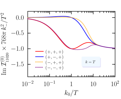
Figure 2: Energy dependence of the type II master integral with $m=n=0\,$, for various statistics at $k=T\,$.

Moving along to the functions $H_{m}\,$, for $m=\{0,1,2\}$, after the frequency sum we have

$$H_{m} = -\sum_{v}\int_{\text{\boldmath$p$},\text{\boldmath$q$}}\ \frac{(2\pi)^{d+1}}{4E_{1}E_{2}}\delta^{(d+1)}(K-v_{1}P-v_{2}Q)$$ (3.5)

$$\times \big{(}\,f_{s_{1}}^{v_{1}}f_{s_{2}}^{v_{2}}-f_{s_{1}}^{-v_{1}}f_{s_{2}}^{-v_{2}}\,\big{)}\,(v_{1}E_{1})^{m}\,,$$

where the summation extends over $v_{1,2}=\pm 1$ [a definition of $f_{s}^{v}$ is given below Eq. (2.2)]. The strategy discussed in Sec. 2 was applied to cover the cases $m\geq 0\,$. Dimensional regularisation is adopted because the related function $G_{m}$ will include a customary ultraviolet divergence: Take $G_{0}$ and $H_{0}$ for instance, which are real and imaginary parts (respectively) of the same function. Their zero temperature limits can be read from

$$\lim_{T\to 0}{\cal J}_{\ 11}^{(0)} = \frac{1}{(4\pi)^{2}}\Big{[}\,\frac{1}{\epsilon}+\kappa+2+{\cal O}(\epsilon)\,\Big{]}\,;$$ (3.6)

$$\kappa \equiv \log\frac{\bar{\mu}^{2}}{K^{2}}-i\,\pi\Theta(K^{2})\,.$$

Branches of the logarithm are made explicit; we write $\log X$ to mean $\log|X|$ . Thus $G_{0}$ bears an ultraviolet divergence and so ${\cal O}(\epsilon)$ terms must be kept in $H_{0}$ when multiplying them together. For that reason we write

$$G_{m} = \,\frac{1}{(4\pi)^{2}}\Big{[}\ G_{m}^{[-1]}\,\Big{(}\,\frac{1}{\epsilon}+\log\frac{\bar{\mu}^{2}}{K^{2}}+2\,\Big{)}+G_{m}^{[0]}+\ldots\ \Big{]}\,,$$

$$H_{m} = -\,\frac{1}{16\pi}\Big{[}\ H_{m}^{[0]}\,\Big{(}\,1+\epsilon\log\frac{\bar{\mu}^{2}}{K^{2}}\,\Big{)}+\epsilon\,H_{m}^{[1]}+\ldots\ \Big{]}\,,$$ (3.7)

to make the dependence on the scale $\bar{\mu}$ explicit. Setting $d=3$ in (3.5) allows us to find $H_{m}^{[0]}$: With help from the moments $\psi^{(m)}$, provided in Eq. (LABEL:psi) of Appendix A, one can express

$$H_{m}(K;s_{1},s_{2})\big{|}_{\epsilon\to 0}=-k_{0}^{m}\,\psi^{(m)}_{s_{1},s_{2}}\,\big{/}\,(16\pi)\ .$$

Thus $H_{m}^{[0]}=k_{0}^{m}\psi_{s_{1},s_{2}}^{(m)}$ is easily read off. Also needed are $G_{0}^{[-1]}=1$ and $G_{1}^{[-1]}=\tfrac{1}{2}k_{0}\,$. The order $\epsilon$ terms $H_{m}^{[1]}$ are presented in Appendix B, as is the function $G_{m}^{[0]}$ for $m=\{0,1\}\,$.

Turning to the class III integral, according to Eq. (3.3) it can be written

$$\hbox{Im}\ {\cal I}_{11011}^{(m,n)}\ =\ \frac{-1}{4(4\pi)^{3}} \Big{[} G_{m}^{[-1]}H_{n}^{[0]}\Big{(}\,\frac{1}{\epsilon}+2\log\frac{\bar{\mu}^{2}}{K^{2}}+4\,\Big{)}$$

$$- \big{(}2\,G_{m}^{[-1]}-G_{m}^{[0]}\big{)}H_{n}^{[0]}+G_{m}^{[-1]}H_{n}^{[1]}+\,{\rm sym.}\,\Big{]}\,,$$

where the last term is from a symmetry as specified in (3.3). The first line above includes all divergences and yields the entire result for $T=0\,$. The second line is purely a finite thermal function which is not present in vacuum. Note that the divergent first line is also a function of the temperature and we omit it in Fig. 3, where the master integral is displayed.

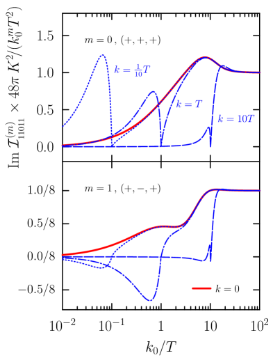
Figure 3: The finite part of the type III master integral, as a function of energy. We show here, for $k=\{0,\tfrac{1}{10},1,10\}T\,$, the two cases $m=0$ (upper) and $m=1$ (lower).

On the light cone, a logarithmic singularity in this thermal part may arise from $\psi\,$. This divergence is softened by the extra weight $K^{2}/T^{2}$ that was used in Fig. 3, and the plotted function is zero at $k_{0}=k\,$. We note that if $s_{0}=1$ (implying $s_{1}=s_{4}$ and $s_{2}=s_{5}$), some simplifying relations hold

$${\cal I}_{11011}^{(1)}\ =\ {\cal I}_{11011}^{(0,1)}\ =\ \frac{k_{0}}{2}\,{\cal I}_{11011}^{(0)}\,.$$

4 Diagram IV (setting sun)

We now consider the first genuine two-loop structure, specifically the integral ${\cal I}^{(0)}_{11100}\,$, which gives e. g. the first non-zero contribution to the imaginary part of the self energy in a scalar $\varphi^{4}$-theory Ramond . Another master of the same class, ${\cal I}^{(0)}_{01110}=0\,$, is identically zero due to integration by parts identities Schroder . The ‘setting sun’ graph is given in vacuum by

$$\lim_{T\to 0}\,{\cal I}^{(0)}_{11100}\!\! = \!\frac{-K^{2}}{4(4\pi)^{4}}\Big{[}\,\frac{1}{\epsilon}+2\,\kappa+\frac{13}{2}+{\cal O}(\epsilon)\,\Big{]}\,,\quad$$ (4.1)

where $\kappa$ was introduced in Eq. (3.6). This vacuum result has an imaginary part for $K^{2}>0$, associated with the threshold for massless particle production. In a thermal medium, the Landau-damping mechanism explains why this imaginary part also builds up below the light cone Wang1995qf . Explicitly,

$$\hbox{Im}\ {\cal I}^{(0)}_{11100} = \sum_{v}\int_{\text{\boldmath$p$},\text{\boldmath$q$},\text{\boldmath$r$}}\frac{(2\pi)^{6}}{8E_{1}E_{2}E_{3}}$$

$$\times \delta^{(4)}(K-v_{1}P-v_{2}Q-v_{3}R)\,\Big{(}\ f_{s_{1}}^{v_{1}}f_{s_{2}}^{v_{2}}f_{s_{3}}^{v_{3}}-f_{s_{1}}^{-v_{1}}f_{s_{2}}^{-v_{2}}f_{s_{3}}^{-v_{3}}\ \Big{)}\,,$$

where $f_{s}^{v}$ was defined just below (2.2) and takes the arguments at energies $E_{1}=|\text{\boldmath$p$}|$, $E_{2}=|\text{\boldmath$q$}|$ and $E_{3}=|\text{\boldmath$r$}|$ which are on-shell. This integral is labelled ‘f’ in Ref. laine2 .

Let us clarify the physical content of Eq. (4). The sum over the signs $v_{i}=\pm 1$ enumerates eight distinct physical interactions, with external momentum $K=(k_{0},\text{\boldmath$k$})$ . We denote the corresponding fields $\phi_{i}$ for argument’s sake with $s_{i}=+1$. As an example, the term with $v_{1}=v_{2}=v_{3}=+1$ represents the probability for decay $\phi_{0}\to\phi_{1}\phi_{2}\phi_{3}$, with a statistical weight of $(1+n_{{}_{B}})(1+n_{{}_{B}})(1+n_{{}_{B}})$ for spontaneous emission, minus the probability for creation $\phi_{1}\phi_{2}\phi_{3}\to\phi_{0}$, with a weight $n_{{}_{B}}n_{{}_{B}}n_{{}_{B}}$ for absorption. There are many other processes, such as $\phi_{0}\phi_{2}\phi_{3}\to\phi_{1}$ minus $\phi_{1}\to\phi_{0}\phi_{2}\phi_{3}$ and so on Weldon1983jn .

Equation (4) may be simplified into a two-dimensional integral (now for general $s_{i}$)

$$\hbox{Im}\ {\cal I}^{(0)}_{11100} = \frac{n_{0}^{-1}}{(4\pi)^{3}}\int\!dp\,dq\ W_{\rm I\!V}(p,q)\ n_{1}\,n_{2}\,n_{3}\ ,$$ (4.3)

where we abbreviated $n_{i}=s_{i}n_{s_{i}}\,$ and agree that the arguments of the distribution functions may be negative. The ‘kernel’ $W_{\rm I\!V}$ (defined below) also depends on $k_{0}$ and $k\,$, but not on the temperature. The momentum moduli $p$ and $q$ have been generalised to negative values, which implicitly incorporates the sum over the signs $\{v_{i}\}$. And the statistical weight has accordingly been re-expressed using

$$f_{s_{1}}^{+}f_{s_{2}}^{+}f_{s_{3}}^{+}-f_{s_{1}}^{-}f_{s_{2}}^{-}f_{s_{3}}^{-} = \ n_{0}^{-1}\,n_{1}\,n_{2}\,n_{3}\ ,$$ (4.4)

An explanation that starts with Eq. (4) is given in appendix C, where we also show how to calculate $W_{\rm I\!V}$ from kinematic constraints. Here we simply state the result:

$$W_{\rm I\!V}(p,q)\ =\ \frac{1}{2k} \Big{\{} |p-k_{+}|+|q-k_{+}|-|p+q-k_{+}|$$

$$- |p-k_{-}|-|q-k_{-}|+|p+q-k_{-}|-\min[k_{0},k]\ \,\Big{\}}\,,$$

where $k_{\pm}=(k_{0}\pm k)/2\,$ are the light cone momenta.

Of note is that $W_{\rm I\!V}(p,q)\simeq p/k$ for $p\to 0$, which suppresses the log divergence from $n_{{}_{B}}(p)$ . Furthermore, $W_{\rm I\!V}=0$ in regions that are kinematically forbidden, providing limits on the $p$ and $q$ integrals. Continuity of $\hbox{Im}\ {\cal I}^{(0)}_{11100}$ at $k_{0}=k$ follows from the very same property in (4). We note that the limit $k\to 0$ is also well-defined and leads to ${W_{\rm I\!V}=\hbox{sgn}\text{\boldmath$($}\,pq(k_{0}-p-q)\,\text{\boldmath$)$}}$ where it has non-zero support.

The statistical factor (4.4) includes the vacuum contribution for $v_{1}=v_{2}=v_{3}=+1\,$, i.e. where $p$ and $q$ are positive and $p+q<k_{0}\,$. It is the leading term in Eq. (4.4), after expanding in combinations of the distribution functions

$$f_{s_{1}}^{+}f_{s_{2}}^{+}f_{s_{3}}^{+}-f_{s_{1}}^{-}f_{s_{2}}^{-}f_{s_{3}}^{-}=1+\textstyle\sum_{i}n_{i}+\sum_{i<j}n_{i}n_{j}\ .$$

In Fig. 4, the energy dependence of $\hbox{Im}\ {\cal I}_{11100}^{(0)}$ is shown for $k=\{0,\tfrac{1}{10},1,10\}\times T$. Here the vacuum result (4.1) was subtracted, i. e. we actually plot

$$\hbox{Im}\ {\cal I}_{11100}^{(0)}-\Theta(K^{2})\,\frac{K^{2}}{8(4\pi)^{3}}\,.$$ (4.6)

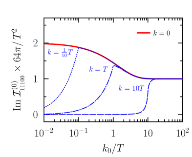
Figure 4: The imaginary part of the scalar self energy (with $s_{i}=+1$), according to Eq. 4.6. Shown here is the dependence on $k_{0}$ for various values of the external momentum.

Because the master integrals are holomorphic in the upper half of the complex $k_{0}$-plane, (4) is an odd function of real energies. (Meaning, in particular, that it is zero for $k_{0}=0\,$.) The exception, for massless particles, occurs when $\text{\boldmath$k$}=0$ so that there is an essential singularity at $k_{0}=0$ Weldon2001vt . Hence the zero momentum curve in Fig. 4 is finite for $k_{0}\to 0$ and not equal to the same limit at fixed $|\text{\boldmath$k$}|>0\,$.

4.1 Kinematics

The region(s) where Eq. (4) provides non-zero support for $W_{\rm I\!V}$ can be understood by elementary kinematic reasoning. It is necessary to belabour this point because the argument will reveal why it holds in general for the real corrections. To illustrate, we first consider the simpler case $k\to 0$ and then explain what happens when $k<k_{0}$ and $k>k_{0}$ separately.

The function $W_{\rm I\!V}$ is not Lorentz invariant – if it were, we could perform the whole calculation in the rest frame. Nevertheless, specialising to $k=0$ will be useful as a starting point. For example, in the channel with $v_{1}=v_{2}=v_{3}=+1$ we require vectors $p$ and $q$ that satisfy

$$k_{0} = |\text{\boldmath$p$}|+|\text{\boldmath$q$}|+|\text{\boldmath$p$}+\text{\boldmath$q$}|\,.$$ (4.7)

Clearly $p+q\leq k_{0}$ in general, with equality if and only if $\text{\boldmath$p$}=-\text{\boldmath$q$}$ and $|\text{\boldmath$p$}|=\frac{1}{2}k_{0}$. Moreover, by the triangle inequality we have $|p-q|<|\text{\boldmath$p$}+\text{\boldmath$q$}|<p+q$ (here $p,q>0$). The upper limit thus gives $\frac{1}{2}k_{0}<p+q$, while the lower limit leads to $p<\frac{1}{2}k_{0}$ if $p>q$ and $q<\frac{1}{2}k_{0}$ if $p<q$. That defines the relevant domain in the $(p,q)$-plane; see ‘1’ in Fig. 5, where $W_{\rm I\!V}=+1$.

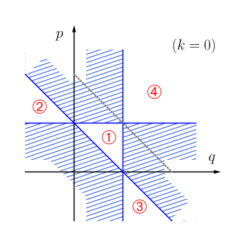
Figure 5: The boundaries to the integration regions for the four (real) corrections. Each region corresponds to a physical process, e. g. ‘1’ is described in the paragraph below (4). The dashed line represents momenta that satisfy $p+q=k_{0}\,$.

If $v_{1}=v_{2}=+1=-v_{3}$, instead of (4.7) we need

$$k_{0}=|\text{\boldmath$p$}|+|\text{\boldmath$q$}|-|\text{\boldmath$p$}+\text{\boldmath$q$}|\,.$$ (4.8)

This time $p+q\geq k_{0}$ and the very same triangle inequalities give $p>\frac{1}{2}k_{0}$ if $q>p$ and $q>\frac{1}{2}k_{0}$ if $q<p$. Similar results hold if $v_{3}=+1$ and if exactly one of $v_{1}$, $v_{2}$ is equal to $-1$. However if two or more of $\{v_{1},v_{2},v_{3}\}$ are negative, the equivalent of (4.7) cannot be satisfied (for $k_{0}>0$). Hence in the sum over $\{v_{i}\}$, only half of the summands contribute.

This is summarised by the wedge-shaped regions ‘2’, ‘3’ and ‘4’ in Fig. 5. In each of these three regions, $W_{\rm I\!V}=-1$. Although they include arbitrary large momenta (in absolute value), those much larger than the temperature are cut off by the thermal distribution functions.

We now consider $k>0$, but still less than $k_{0}$ so that $k_{-}=\frac{1}{2}(k_{0}-k)$ is positive. The external vector $k$ now plays a role, i. e. (4.7) is supplanted by

$$k_{0} = |\text{\boldmath$p$}|+|\text{\boldmath$q$}|+|\text{\boldmath$k$}-\text{\boldmath$p$}-\text{\boldmath$q$}|\,.$$ (4.9)

Of course $p+q\leq k_{0}$ still holds, but now equality can occur for all $q\in[k_{-},k_{+}]$. The triangle inequality gives $k+|\text{\boldmath$p$}+\text{\boldmath$q$}|>|\text{\boldmath$k$}-\text{\boldmath$p$}-\text{\boldmath$q$}|$, and therefore

$$2k_{-}=(k_{0}-k) < |\text{\boldmath$p$}|+|\text{\boldmath$q$}|+|\text{\boldmath$p$}+\text{\boldmath$q$}|\ <\ 2(p+q)\,.$$

Hence the lower bound on $p+q$ is diminished to $k_{-}$. Similarly, the other side of the triangle inequality gives $|\text{\boldmath$k$}-\text{\boldmath$p$}-\text{\boldmath$q$}|>|\text{\boldmath$p$}+\text{\boldmath$q$}|-k$. That produces $k_{+}\geq\max(p,q)$, which is higher than the upper bound for $k=0$. Generalising to other channels is trivial; see Fig. 6. These restrictions are reflected in the function $W_{\rm I\!V}$. In the ‘new’ bands that open up for $p,q,r\in[k_{-},k_{+}]$, tilted facets make $W_{\rm I\!V}$ a continuous function compared to the case where $k=0$. Moreover, the exact form (4) renders the product of distribution functions integrable.

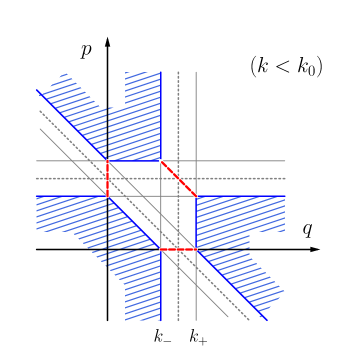
Figure 6: As before, now with $0<k<k_{0}$. The red dashed lines give the boundaries between different channels; i. e. where one of $p$, $q$ or $r=(k_{0}-p-q)$ changes sign.

As $k$ is increased beyond $k_{0}$, the virtuality $K^{2}=4k_{+}k_{-}$ becomes negative. The channel with $v_{1}=v_{2}=v_{3}=+1$ ceases to be accessible; conservation of energy (4.9) cannot be satisfied if $k_{0}<k$. This simply means that there is no vacuum contribution below the light cone, as expected.

New wedges open up in the $(p,q)$-plane – they correspond to having exactly two of $\{v_{1},v_{2},v_{3}\}$ equal to $-1$. In Fig. 7 they are labelled ‘5‘, ‘6’ and ‘7’. Regions ‘2’, ‘3’ and ‘4’ are carried over from the case $k<k_{0}$, with modified boundaries: For example in ‘2’, the same triangle inequality as before gives $|\text{\boldmath$q$}|<-k_{-}$ . Region ‘5’ has $v_{1}=v_{2}=-1$ and $v_{3}=+1$ , so in some sense it is the intersection of ‘2’ and ‘3’. In ‘5’ we have $p$ and $q$ negative such that $p+q<k_{-}$ . (And there are similar constraints for ‘6’ and ‘7’.) We note that adjacent regions are separated by lines where $p$, $q$ or $r$ is zero. These boundaries are important because they mark the location of potential singularities coming from bosonic distribution functions.

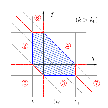
Figure 7: As before, now with $k>k_{0}$ so that $k_{-}<0$. (The blue hatched region is forbidden by kinematics. It is, incidently, also where the vacuum contribution comes from.)

The expression in (4) can be simplified in each of the demarcated regions discussed for $k_{0}>k$ and $k_{0}<k\,$. In the former case, we recover Eqs. (33-43) of Appendix B in Ref. laine2 (with an adjustment in variables, namely $p\to k_{0}-p$). For the more complicated master integrals still to be studied, the same regions must be considered, though the kernel functions will be different. Hence, the foregoing analysis serves to spell out what must be included for the task of numerical integration.

5 Diagram V (the squint)

In the previous section there is only one ‘contribution’ to the imaginary part: all of the three internal energies are set to their on-shell value giving (4). But more generally, the discontinuity may always be written in terms of products of two amplitudes that are separated by on-shell ‘cut’ propagators Weldon1983jn . For classes V and VI, there is more than one way to do this; see Fig. 8. These contributions, which may be readily identified after carrying out the Matsubara sums, are separately infrared divergent. They differ by one extra loop momentum being on-shell in the real case, yielding a tree-level decay that may be treated in a similar manner to that of the previous section. The virtual correction has an internal loop due to one fewer final state particle than before and includes a two-body phase space integration. The latter is also ultraviolet divergent, seen in the vacuum result [$\kappa$ was introduced in Eq. (3.6)]

$$\lim_{T\to 0}\,{\cal I}^{(0)}_{11110} = \frac{1}{(4\pi)^{4}}\Big{[}\ \frac{1}{2\epsilon^{2}}\,+\,\frac{2\kappa+5}{2\epsilon}\,+\,\kappa(\kappa+5)+\,\frac{19}{2}\,-\,\frac{\pi^{2}}{12}\,+\,{\cal O}(\epsilon)\,\Big{]}\,,$$ (5.1)

which, for $K^{2}$ positive, contains an imaginary part $\propto 1/\epsilon\,$. This divergence will then acquire a temperature dependence in the medium. When assembled together, these infinite parts cancel in actual observables.

Figure 8: Cut type II diagrams. Real (a) and virtual (b).

The two terms shown in Fig. 8 also have separate collinear divergences which exactly compensate only in their sum. This cancellation is somewhat intricate at finite temperature and affirms the Kinoshita-Lee-Nauenberg (KLN) theorem, in this case applied to individual graphs kln1 ; kln2 . The amplitude (a) in Fig. 8 may contain a large ‘eikonal factor’ if the denominator of an internal line is zero,

$$L^{2}\ =\ K^{2}-2(v_{1}p)\,\big{(}\,k_{0}-k\cos\theta_{kp}\,\big{)}\ \approx\ 0\,,$$ (5.2)

where $\theta_{kp}$ is the angle between $p$ and $k$. Such configurations exhibit two collinear outgoing (massless) particles that should be removed from the definition of a physical production rate, i. e. by including (b) from Fig. 8. The conditions for some $\theta_{kp}$ to satisfy Eq. (5.2) are inferred according to the sign of $K^{2}\,$: If $K^{2}>0$ then $(v_{1}p)$ must be in the interval $\Omega=[k_{-},k_{+}]$ (spanned by the light cone momenta). While if $K^{2}<0$, (5.2) can be satisfied if and only if $(v_{1}p)$ is in the complementary region $\Omega^{c}=\mathbb{R}\backslash\Omega\,$.

A fictitious mass $\lambda\,$ (for the momentum $R$) is convenient to use as a calculational tool ItzyksonZuber . It prevents $L^{2}\to 0$ in (5.2) and proves that the whole expression

$$\hbox{Im}\ {\cal I}^{(m,n)}_{11110} \!\!\!\!\!=\frac{n_{0}^{-1}}{(4\pi)^{3}}\int\!dp\,p^{m}\,\Big{[}$$ (5.3)

$$\int\!dq \!\!\!\!\!\!q^{n}\,W_{\rm V}(p,q\,;\lambda)\ n_{1}n_{2}n_{3}+U^{(n)}_{\rm V}(p\,;\lambda)\ n_{1}n_{4}\ \Big{]}\,,$$

is rendered finite as $\lambda\to 0\,$. [See ahead (6.3) for the abbreviations $n_{i}\,$.] The first term above represents the real correction, and involves the thermal weight (4.4) from before. Virtual corrections lead to the second term and depend on the mass $\lambda$ so as to compensate for the contingent singularity in the first. Equation (5.3) is valid for $m,n\leq 1$, otherwise there could be more terms.

We may obtain $W_{\rm V}(p,q\,;\lambda)$ by the techniques laid out in Appendix C. A compact formula for it can be given with the help of some funny notation:

$$\hat{p}=\max\big{[}\,k_{-},\,\min[k_{+},p]\,\big{]}\,.$$

To also indicate whether $p$ is in the interval $\Omega=[k_{-},k_{+}]$, we define

$$o_{p}=\Theta\big{(}(k_{+}-p)(p-k_{-})\big{)}=\left\{\begin{array}[]{ll}1&{\rm if}\ p\in\Omega\\ 0&{\rm otherwise.}\end{array}\right.$$

Thus the complementary set $\Omega^{c}=\mathbb{R}\backslash\Omega$ contains $p$ if the value of $\bar{o}_{p}=1-o_{p}\,$ is equal to unity. Using $o_{p}$ and $\bar{o}_{p}$ will signal terms that are included or not, depending on the relative ordering of $k\,$, $k_{0}$ and $p\,$. With these definitions, and regulating through $\lambda\to 0$, the weight function can be expressed as

$$W_{\rm V}(p,q;\lambda)\ =\ \frac{1}{4k\,\ell}\!\! \Big{\{} \log W_{\rm V}^{\prime}+\Theta(k_{-})\log W_{\rm V}^{\prime\prime}$$

$$+ \bar{o}_{p}\log W_{\rm V}^{\prime\prime\prime}+\big{(}\Theta(k_{-})-\bar{o}_{p}\big{)}\log\frac{4\ell r}{\lambda^{2}}\,\Big{\}}\,,$$

where we have introduced the ratios

$$\displaystyle W^{\prime}_{\rm V}=\frac{(\ell-\hat{q})(\ell-\hat{r})}{\hat{q}\,\hat{r}}\,,\qquad W^{\prime\prime}_{\rm V}=\frac{k_{-}}{p-k_{+}}\,,\qquad\displaystyle W^{\prime\prime\prime}_{\rm V}=\frac{k_{0}-\hat{p}}{p-\hat{p}}\,.$$

An explicit log-divergence in (5) lingers if $p\in\Omega$ (for $k_{0}>k$) or if $p\in\Omega^{c}$ (for $k_{0}<k$). This implies that it is too soon to set $\lambda=0$ in those domains of the $(p,q)$-plane and brings us to incorporate the missing virtual pieces.

Again deferring details to Appendix C, we write, for $\lambda\to 0$,

$$U^{(0)}_{\rm V}(p\,;\lambda)=\frac{\bar{o}_{p}-\Theta(k_{-})}{4k}\!\! \Big{[}$$

$$- \frac{1}{\ell}\int_{-\infty}^{+\infty}\!\!dq\Big{\{}\,\frac{n_{2}n_{3}}{n_{4}}\log\frac{\lambda^{2}}{4\ell q}+s_{3}\hbox{sgn}(r)n_{s_{3}}\big{(}|r|\big{)}\log\frac{q^{2}}{r^{2}}\,\Big{\}}$$

$$+ \frac{1}{\epsilon}+2\log\frac{\bar{\mu}^{2}}{K^{2}}+\log\frac{K^{2}k^{2}}{4\ell^{2}(p-k_{-})(p-k_{+})}+2\,\Big{]}\,.$$

This reveals how the anticipated ultraviolet divergence in (5.1) emerges from the loop in (b) of Fig. 8. At the same time, it can be seen that the $\lambda$-dependence in (5.3) cancels for $\lambda=0$, with the logarithmic mass singularities compensating perfectly,

$$\log\frac{4\ell r}{\lambda^{2}}+\log\frac{\lambda^{2}}{4\ell q}=\log\frac{r}{q}\,,$$

and in exactly the domains where (5.2) is satisfied. They coalesce in this way both above and below the light cone.

For the purpose of plotting, we subtract a piece that is ultraviolet divergent from (5.3) and coincides with its vacuum result for $T=0$. What remains is thus finite and proportional to $T^{2}$ for large photon virtualities, see Fig. 9. The function is continuous across the light cone unless it diverges there, in which instance the singularity is the same if $k_{0}\to k$ is approached from either above or below. That is why, in Fig. 9, we multiply the whole function by $|K^{2}|$ which is enough to render the blow-up finite on the light cone. (It also gives the whole master integral a dimension of $T^{2}$.) To be clear, and following laine2 (in which this master is labelled ‘h’), the part subtracted is

$$\hbox{Im}\ {\cal I}^{(0)}_{11110}\Big{|}_{\rm div.} = -\frac{\psi^{(0)}_{s_{1},s_{4}}}{4(4\pi)^{3}}\Big{(}\,\frac{1}{\epsilon}+2\log\frac{\bar{\mu}^{2}}{K^{2}}+5\,\Big{)}\,,$$ (5.6)

where $\psi$ is defined in Eq. LABEL:psi of the appendices. The large $k_{0}$-expansion of the whole master integral is given in Eq. (D.12).

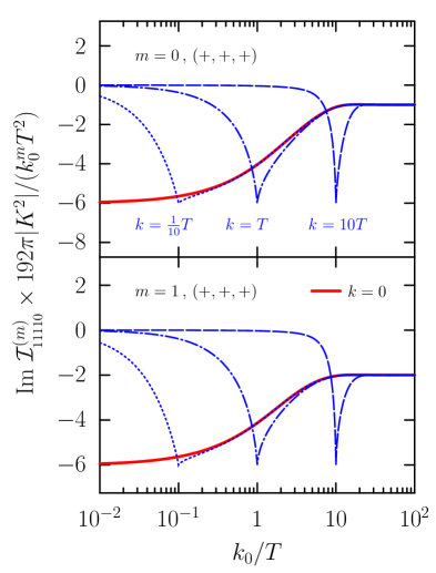
Figure 9: The imaginary part of the type V master (with all $s_{i}=+1$), in units of the asymptotic result. Shown here is the dependence on $k_{0}$ for various values of the external momentum, including $k=0$.

Next, let us consider the case $m=1$ and $n=0\,$. The modification in (5.3) is trivial; only an extra factor of $p$ needs to be included in the integrand. The kernels $W_{\rm V}$ and $U_{\rm V}^{(0)}$ are unaffected and hence the $\lambda$-dependence (and ultimate lack thereof) is the same as before. For plotting in Fig. 9, we subtract

$$\hbox{Im}\ {\cal I}^{(1)}_{11110}\Big{|}_{\rm div.} = -\frac{k_{0}\psi^{(1)}_{s_{1},s_{4}}}{4(4\pi)^{3}}\Big{(}\,\frac{1}{\epsilon}+2\log\frac{\bar{\mu}^{2}}{K^{2}}+\frac{11}{2}\,\Big{)}$$ (5.7)

from the result. The shape is similar to $\hbox{Im}\ {\cal I}^{(0)}_{11110}\,$, but ratios of the large-$k_{0}$ limit to its value on the light cone are different.

For $m=0$ and $n=1\,$, the virtual parts need to be reconsidered. The result, with details available in Appendix C, can be written, for $\lambda\to 0\,$,

$$U^{(1)}_{\rm V}(p\,;\lambda)=\frac{\bar{o}_{p}-\Theta(k_{-})}{4k}\!\! \Big{[}$$

$$- \int_{-\infty}^{+\infty}\!dq\,\frac{q}{\ell}\Big{\{}\,\frac{n_{2}n_{3}}{n_{4}}\log\frac{\lambda^{2}}{4\ell q}+s_{3}\hbox{sgn}(r)n_{s_{3}}\big{(}|r|\big{)}\log\frac{q^{2}}{r^{2}}\,\Big{\}}$$

$$+ \frac{\ell}{2}\,\Big{\{}\,\frac{1}{\epsilon}+2\log\frac{\bar{\mu}^{2}}{K^{2}}+\log\frac{K^{2}k^{2}}{4\ell^{2}(p-k_{-})(p-k_{+})}+1\,\Big{\}}\ \Big{]}\,.$$

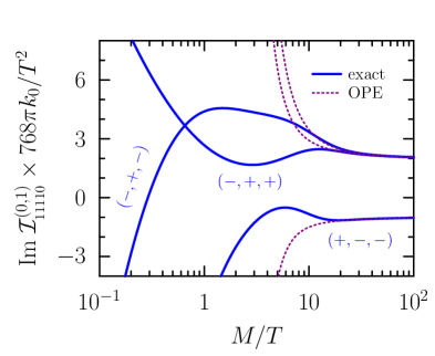
Figure 10: Here we display the type V master with $m=0$ and $n=1\,$, minus the divergent part.Various statistical configurations are shown with $s_{0}\neq s_{1}$ (so that these cannot be reduced to a linear combination of master integrals with $n=0$). The first two orders from the OPE asymptotics, Eq. (D), start agreeing from about $M\mathrel{\hbox to0.0pt{\lower 2.5pt\hbox{$\sim$}\hss}\raise 1.99997pt\hbox{$>$}}30T\,$.

Figure 10 displays the result as a function of positive invariant mass $M=\sqrt{k_{0}^{2}-k^{2}}\,$. We have followed Refs. laine1 ; laine2 by using $M$ to define

$$k_{\rm ave}^{2}(M) \equiv \frac{3MTK_{3}\big{(}M/T\big{)}}{K_{2}\big{(}M/T\big{)}}\,,$$ (5.9)

as a proxy for the average three momentum squared. ($K_{\nu}$ are modified Bessel functions.) This quantity assumes Boltzmann distribution functions to average $k^{2}$ for a fixed mass. The curves shown in Fig. 10 use $k\to\sqrt{k_{\rm ave}^{2}(M)}$ as a rather crude substitute for ‘typical’ momenta. As $M\to 0\,$, we note the clear log-divergent behaviour of the master integral for the statistics shown in the figure.

The divergent piece that was subtracted is given by [note the ordering of $s_{4}$ and $s_{1}$ on $\psi^{(1)}$ ]

$$\hbox{Im}\ {\cal I}^{(0,1)}_{11110}\Big{|}_{\rm div.} = -\frac{k_{0}\psi^{(1)}_{s_{4},s_{1}}}{8(4\pi)^{3}}\Big{(}\,\frac{1}{\epsilon}+2\log\frac{\bar{\mu}^{2}}{K^{2}}+\frac{9}{2}\,\Big{)}\,.$$

We have also checked numerically that $\hbox{Im}\ {\cal I}_{11110}^{(0,1)}=\frac{1}{2}\big{(}k_{0}\,\hbox{Im}\ {\cal I}_{11110}^{(0)}-\hbox{Im}\ {\cal I}_{11110}^{(1)}\big{)}$ provided $s_{2}=s_{3}\,$. This relation follows by a shift of integration variables, but it seems difficult to discern this rule by simply looking at the explicit form of the integrand.

In Sec. 2 we listed among the type V integrals, one with a propagator of negative power $e=-1\,$. It is significant because of a logarithmic divergence for $K^{2}\ll T^{2}$ that makes it dominant over those that are merely finite on the light cone (when scaled by $K^{2}$ to have the appropriate dimension). This brings about its appearance in many applications. Moreover, the continuity across the light cone (that some previous masters seemed to enjoy) is no longer guaranteed. This issue reveals itself explicitly in the QCD corrections to the photon spectral function (2.2) [used in (1.1)],

$$\hbox{Im}\,\Pi_{\mu}^{\ \mu} \simeq e^{2}g^{2}\,T^{2}\ \frac{NC_{\mbox{\rm\scriptsize F}}}{16\pi}\big{[}\,1+2\,n_{{}_{-}}(k_{0})\,\big{]}\log\frac{T^{2}}{K^{2}}$$ (5.10)

for $K^{2}\ll T^{2}$ Baier1988 ; Altherr1989 ; Gabellini1989 . This is the singularity alluded to in the Introduction, which mandates screening effects to be incorporated through resummation. The log-singularity on the light cone can be traced back to the integral we are about to discuss.

Let us consider the particular combination of master integrals defined by

$${\cal I}_{11110}^{\text{\,\large$\star$}} \equiv {\cal I}_{10110}^{(0)}+K^{2}\,{\cal I}_{11110}^{(0)}-{\cal I}_{1111(-1)}^{(0)}$$

$$= {\hbox{$\textstyle\sum$}\!\!\!\!\!\!\!\int\,}_{\!\!\!\!\raise-1.50694pt\hbox{$\scriptstyle{\,P,Q}$}}\frac{2\,K\cdot Q}{P^{2}\,Q^{2}\,(K-P-Q)^{2}\,(K-P)^{2}}\,.$$

(This one is labelled by ‘h^′ ’ in Ref. laine2 .) After carrying out the Matsubara sum, one arrives at Eq. (C) in the Appendix. Along the same lines as (5.3), this can be expressed by

$$\hbox{Im}\ {\cal I}_{11110}^{\text{\,\large$\star$}}\,=\,\frac{n_{0}^{-1}}{(4\pi)^{3}}\int\!dp\!\! \Big{[} \int\!dq\,W_{\text{\large$\star$}}(p,q\,;\lambda)\,n_{1}n_{2}n_{3}+U_{\text{\large$\star$}}(p\,;\lambda)\,n_{1}n_{4}\ \Big{]}\ ,$$ (5.12)

where the two terms are the real and virtual parts respectively. The first weight includes the same manner of $\lambda$-dependence as that previously defined in (5), which allows the previous argument to be partially recycled here. To explicitly define $W_{\text{\large$\star$}}\,$, let

$$g(x)\equiv(k_{0}^{2}+k^{2}-2k_{0}p-2k\ell x)^{2}\,.$$

Accordingly, in the first summand of (5.12), we have

$$W_{\text{\large$\star$}}(p,q;\lambda)\,=\,\frac{q}{\ell}\,\Big{\{}K^{2}\,W_{\rm V}-\frac{\hbox{sgn}(p)}{4k\,\ell}\big{(}\,\sqrt{g(x_{2}^{\rm max})}-\sqrt{g(x_{2}^{\rm m\i n})}\,\big{)}\ \Big{\}}\,.$$ (5.13)

The arguments of $g$ are defined in Appendix C; see Eq. (C.9). Virtual corrections in (5.12) require the function

$$U_{\text{\large$\star$}}(p\,;\lambda) = \frac{1}{\ell}\,K^{2}U_{\rm V}^{(1)}+\frac{\bar{o}_{p}-\Theta(k_{-})}{4k}\big{(}\,K^{2}-2\ell\,k_{0}\,\big{)}$$ (5.14)

$$\times \Big{[}\,1-\frac{2}{\ell^{2}}\int_{-\infty}^{+\infty}\!\!dq\,q\ \frac{n_{2}n_{3}}{n_{4}}\,\Big{]}\,.$$

We see that the auxiliary mass $\lambda$ enters only in the previously defined functions, $W_{\rm V}$ and $U_{\rm V}^{(1)}$, so that the pattern of cancellation is unchanged and allows us to set $\lambda=0\,$. The divergent piece that we choose to subtract is

$$\hbox{Im}\ {\cal I}^{\text{\large$\star$}}_{11110}\Big{|}_{\rm div.} = -\frac{\psi^{(0)}_{s_{1},s_{4}}}{8(4\pi)^{3}}\Big{(}\,\frac{1}{\epsilon}+2\log\frac{\bar{\mu}^{2}}{K^{2}}+\frac{9}{2}\,\Big{)}\,.$$

We have checked numerically that $\hbox{Im}\ {\cal I}_{11110}^{\text{\large$\star$}}=\frac{1}{2}\big{(}K^{2}\,\hbox{Im}\ {\cal I}_{11110}^{(0)}+\hbox{Im}\ {\cal I}_{11100}^{(0)}\big{)}$ if $s_{2}=s_{3}\,$. As far as the nature of the function across the light cone is concerned in this case, it may be discontinuous if $\hbox{Im}\ {\cal I}_{11110}^{(0)}$ is singular; see the earlier discussion about that master integral. The master $\hbox{Im}\ {\cal I}_{11100}^{(0)}$ is continuous.

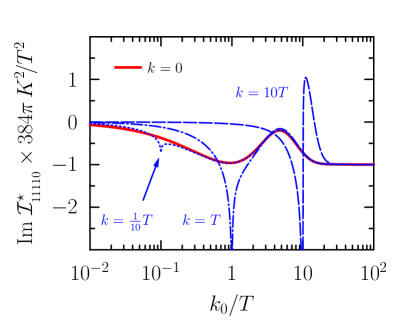
Figure 11: The special master diagram defined in (5), for $s_{0}=+1$ and $s_{1}=s_{2}=-1\,$. With these statistical factors, the function cannot be reduced to any masters already discussed. It also bears a logarithmic divergence on the light cone.

That brings us to the case $s_{2}\neq s_{3}\,$, shown for $s_{0}=+1$ and $s_{1,2}=-1$ in Fig. 11, for which this master integral is a new object. Indeed the outstanding $q$-integral in (5.14) can be found by recalling $s_{4}=s_{2}s_{3}$ and mapping the arguments of the distribution functions to positive values, viz.

$$\int_{-\infty}^{+\infty}\!\!dq\,q\ \frac{n_{s_{2}}n_{s_{3}}}{n_{s_{4}}} = \int_{0}^{\ell}\!\!dq\,q\,+\,2\int_{0}^{\infty}\!\!dq\,q\,\big{(}\,s_{2}n_{s_{2}}(q)-s_{3}n_{s_{3}}(q)\,\big{)}$$

$$= \frac{\ell^{2}}{2}+T^{2}(s_{2}-s_{3})\frac{\pi^{2}}{4}\,.$$

This makes the square brackets in (5.14) a difference between two thermal moments; see (D.20), for the particular statistics $s_{2}$ and $s_{3}\,$. If they are the same, it gives zero. A noteworthy feature is the behaviour for $K^{2}\to 0\,$, where the functions $W_{\text{\large$\star$}}$ and $U_{\text{\large$\star$}}$ simplify. There is a discontinuity due to the latter, cf. Ref. JL , defined by the function’s limit $k_{0}\to k+0^{+}$ minus $k_{0}\to k-0^{+}\,$. For a general statistical configuration, it is given by

$$\hbox{Im}\ {\cal I}^{\text{\large$\star$}}_{11110}\,\Big{|}_{\rm disc.} = T^{2}(s_{3}-s_{2})\,\frac{n_{0}^{-1}}{256\,\pi}\,\int_{-\infty}^{+\infty}\!\!dp\ \frac{n_{1}n_{4}}{k_{0}-p}\,,$$ (5.15)

where the integration is meant in the principal valued sense.

6 Diagram VI (cat’s eye)

The most complicated form of (2.1) that we consider here is $a=b=c=d=e=1\,$, which requires a careful cancellation of real and virtual diagrams. We can deploy the same strategy as in Sec. 5, albeit now with two real and two virtual amplitudes. (Each is related by the symmetry $s_{1}\leftrightarrow s_{4}$ and $s_{2}\leftrightarrow s_{5}\,$.) An auxiliary mass $\lambda$ is again attached to $E_{3}=\sqrt{r^{2}+\lambda^{2}}$ so that collinear singularities can be regulated.

In Ref. laine1 , the function $\hbox{Im}\ {\cal I}_{11111}^{(0)}$ (it was labelled with ‘j’ there) was computed above the light cone. For that case, with $m=n=0\,$, we do not need to worry about ultraviolet divergences. The vacuum result, given by

$$\lim_{T\to 0}\,{\cal I}^{(0)}_{11111} = \frac{6\zeta(3)}{(4\pi)^{4}\,K^{2}}+{\cal O}(\epsilon)\,,$$ (6.1)

is finite and has no imaginary part. The leading contribution to $\hbox{Im}\ {\cal I}^{(0)}_{11111}$ is therefore thermal. Those masters with $m,n\neq 0$ are more complicated, and can have non-zero vacuum parts with ultraviolet divergences.

For $m,n\leq 1\,$, one can directly use (2.3) to express

$$\hbox{Im}\ {\cal I}^{(m,n)}_{11111}=\frac{n_{0}^{-1}}{(4\pi)^{3}} \bigg{[} \int\!dpdq\,p^{m}\,q^{n}\,\Big{(}\,W_{\rm V\!I}(p,q\,;\lambda)n_{1}n_{2}+W_{\rm V\!I}(\ell,v\,;\lambda)n_{4}n_{5}\,\Big{)}\,n_{3}$$ (6.2)

$$+\int\!dp\,p^{m}U_{\rm V\!I}^{(n)}(p\,;\lambda)\,n_{1}n_{4}+\int\!dq\,q^{n}U_{\rm V\!I}^{(m)}(q\,;\lambda)\,n_{2}n_{5}\ \bigg{]}\,.$$

The real (virtual) contributions are in the first (second) line above, inheriting the notation from earlier sections. As before, $p$ and $q$ may take on negative values. Here the arguments of the distribution functions were omitted, they are

$$n_{0} =\ s_{0}n_{s_{0}}(k_{0})$$ , (6.3)

$$n_{1} =\ s_{1}n_{s_{1}}(p)$$ ,

$$n_{2} =\ s_{2}n_{s_{2}}(q)$$ ,

$$n_{3} =\ s_{3}n_{s_{3}}(r) ;\quad r=k_{0}-p-q\,,$$

$$n_{4} =\ s_{4}n_{s_{4}}(\ell) ;\quad\ell=k_{0}-p\,,$$

$$n_{5} =\ s_{5}n_{s_{5}}(v) ;\quad v=k_{0}-q\,.$$

The weight function $W_{\rm V\!I}$ that is needed in (6.2), carrying over some notation from (5.13), reads for $k_{0}>k$ and $\lambda\to 0\,$,

$$W_{\rm V\!I}(p,q;\,\lambda)\ =\ \frac{1}{4kK^{2}r}\!\!\! \Big{\{} \log W_{\rm V\!I}^{\prime}+\bar{o}_{p}\log W_{\rm V\!I}^{\prime\prime}+\bar{o}_{q}\log W_{\rm V\!I}^{\prime\prime\prime}$$

$$+ o_{p}\log\frac{K^{2}r^{2}(p-q)(p-k_{-})}{\lambda^{2}p\ell(q-k_{-})(q-k_{+})}+o_{q}\log\frac{K^{2}r^{2}(p-q)(q-k_{-})}{\lambda^{2}qv(p-k_{-})(p-k_{+})}\,\Big{\}}\,.$$

Below the light cone ($k_{0}<k$), the function should instead be

$$W_{\rm V\!I}(p,q;\,\lambda)\,=\,\frac{1}{4kK^{2}r}\Big{\{}\log W_{\rm V\!I}^{\prime\prime\prime\prime}-\bar{o}_{p}\log\frac{K^{2}r^{2}(p-\hat{p})}{\lambda^{2}p\ell(v-\hat{p})}-\bar{o}_{q}\log\frac{K^{2}r^{2}(q-\hat{q})}{\lambda^{2}qv(\ell-\hat{q})}\ \Big{\}}\,.$$

In Eq. (6) the following ratios were defined:

$$\displaystyle W^{\prime}_{\rm V\!I}=\frac{(\ell-\hat{r})(v-\hat{r})}{(q-\hat{p})(p-\hat{q})}\,,\qquad W^{\prime\prime}_{\rm V\!I}=\frac{p-k_{-}}{p-\hat{p}}\,,$$

$$\displaystyle W^{\prime\prime\prime}_{\rm V\!I}=\frac{q-k_{-}}{q-\hat{q}}\,,\qquad W^{\prime\prime\prime\prime}_{\rm V\!I}=\frac{(\ell-\hat{r})(v-\hat{r})}{pq}\,.$$

We note the appearance of a log-divergence, just where expected and signaled by the coefficients $o_{p}$ and $o_{q}$ . The formulas for $W_{\rm V\!I}$ are symmetric in arguments $p$ and $q\,$, as is (then) the other real correction, which comes from $p\to k_{0}-p$ and $q\to k_{0}-q\,$.

The case $m=2$ and $n=0$ can also be written in the form of (6.2). One way of seeing this, is to follow (2.4) and rewrite

$${\cal I}_{11111}^{(2)}\ =\ {\cal I}_{01111}^{(0)}+{\hbox{$\textstyle\sum$}\!\!\!\!\!\!\!\int\,}_{\!\!\!\!\raise-1.50694pt\hbox{$\scriptstyle{\,P,Q}$}}E_{1}^{2}\Delta_{1}\Delta_{2}\Delta_{3}\Delta_{4}\Delta_{5}\,,$$

where the explicit integrands for the two terms can be found in Appendix C. (After $s_{1}$ is interchanged with $s_{5}\,$ in the first term above.) Equation (6.2) can be recovered after some manipulations of integration variables.

The virtual corrections are triangle diagrams, one of which is given by the second line of (C) in the Appendices. Their calculation is similar to those studied in the previous section and is given explicitly in Appendix C. Taking up the first term in the second line of Eq. (6.2) (the other term follows analogously), for $\lambda\to 0$ it can be expressed by

$$U_{\rm VI}^{(n)}(p;\lambda)\ =\ \frac{\bar{o}_{p}-\Theta(k_{-})}{4kK^{2}}\int\!\!\frac{dq\,q^{n}}{r}\!\! \Big{[} \big{(}n_{2}-n_{5}\big{)}\log\frac{(q-k_{-})(q-k_{+})}{qv}$$

$$+ \frac{n_{2}n_{3}}{n_{4}}\log\frac{\lambda^{2}\ell v}{K^{2}r^{2}}\ -\ \frac{n_{3}n_{5}}{n_{1}}\log\frac{\lambda^{2}pq}{K^{2}r^{2}}\ \Big{]}\ .$$

Together, the last two terms in (6.2) are seen to combine with the real corrections [see (6)] so that the complete expression is $\lambda$-independent.

We show the case $m=n=0$ in Fig. 12, for all bosonic statistics. (This figure confirms Ref. laine1 above the light cone.) The curves appear continuous across the light cone because we multiplied the whole function by $\hbox{sgn}(K^{2})K^{4}=|K^{2}|K^{2}\,$. That supports the symmetrical nature of the discontinuity at $k_{0}=k\,$. No subtraction is necessary for large-$k_{0}\,$, since according to (6.1) the whole master has no imaginary part in vacuum.

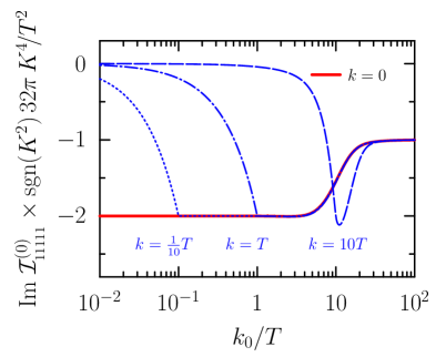
Figure 12: The imaginary part of the type VI master (with $s_{i}=+1$), in units of the asymptotic result. Shown here is the dependence on $k_{0}$ for various values of the external momentum.

If we consider $m=1$ and $n=0\,$, see (D), no vacuum subtraction is necessary. The symmetric case $m=0$ and $n=1$ is obtained by an appropriate exchange of statistics: $s_{1}\leftrightarrow s_{2}$ and $s_{4}\leftrightarrow s_{5}\,$. Moreover, the case $s_{0}=+1$ implies $s_{1}=s_{4}$ and $s_{2}=s_{5}$ which allows a change of integration variables to show $\hbox{Im}\,{\cal I}_{11111}^{(1)}=\frac{1}{2}k_{0}\,\hbox{Im}\,{\cal I}_{11111}^{(0)}$ . We have checked this numerically.

For $m=n=1\,$, there is a leading vacuum term in (D.18). At finite temperature it originates from the two symmetrical virtual expressions. They do not diverge, but we subtract them nonetheless:

$$\hbox{Im}\ {\cal I}^{(1,1)}_{11111} - \frac{\psi^{(0)}_{s_{1},s_{4}}+\psi^{(0)}_{s_{2},s_{5}}}{32(4\pi)^{3}}\ .$$ (6.6)

Based on a numerical study, I conjecture that the discontinuity across the light cone takes the simple form

$$K^{2}\ \hbox{Im}\ {\cal I}^{(1,1)}_{11111}\,\Big{|}_{\rm disc.}=\frac{T^{2}}{512\pi}(s_{1}+s_{2}+2)(s_{3}+1)\,.$$

There thus seems to only be a discontinuity in the statistical configurations: $(+,+,+)\,$, $(-,+,-)$ and $(-,-,+)\,$, the first of which case is shown in Fig. 13, plotted after Eq. (6.6)’s subtraction was made.

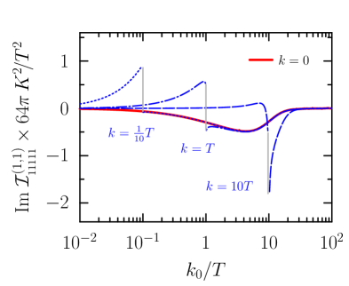
Figure 13: Like Fig. 12, but with $m=n=1$ and with all $s_{i}=+1\,$. The discontinuity is indicated by a vertical line. Large $k_{0}$ behaviour was subtracted according to (6.6).

One needs to be careful for $m=2$ because a genuine ultraviolet divergence must be subtracted. That divergence is temperature dependent and originates from the virtual contribution $U_{\rm VI}^{(2)}(q)\,$. It is equal to

$$\hbox{Im}\ {\cal I}^{(2)}_{11111}\Big{|}_{\rm div.} = -\frac{\psi^{(0)}_{s_{2},s_{5}}}{16(4\pi)^{3}}\Big{(}\,\frac{1}{\epsilon}+2\log\frac{\bar{\mu}^{2}}{K^{2}}+\frac{11}{2}\,\Big{)}\,,$$ (6.7)

which we subtract for plotting purposes. (For the related master integral with $m=0$ and $n=2\,$, one replaces $s_{2}\to s_{1}$ and $s_{5}\to s_{4}$ in the above.) Figure 14 depicts $\hbox{Im}\ {\cal I}^{(2)}_{11111}$ as a function of energy. Although not shown, this quantity also seems to be discontinuous across the light cone. The figure uses an average three momentum-squared, defined in Eq. (5.9), and the energy $k_{0}=\sqrt{M^{2}+k_{\rm ave}^{2}}\,$.

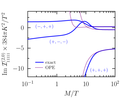
Figure 14: The dependence of the type VI master, with $m=2$ and $n=0\,$, on the invariant mass. An ultraviolet divergent part was subtracted, see Eq. (6.7).

7 Results and conclusions

We have computed a list of spectral functions that originate from self-energy diagrams with two loops, generalising the results of Refs. laine1 ; laine2 to below the light cone and considering a larger set of master integrals with $m,n>0\,$. In so doing, we have separated the ultraviolet divergence where appropriate and shown how to determine the finite remainder numerically. Validity of the KLN theorem was explicitly demonstrated in Secs. 5 and 6, by careful analysis of the collinear phase space. We considered any arrangement of propagating bosons or fermions allowed by the diagram’s topology. The code used for our numerical evaluation is publicly available at Ref. code .

Returning at last to the QCD corrections for the photon spectral function, which was our original motivation, the imaginary parts of Eqs. (2.2) and (2.2) can now be evaluated. Firstly, all the temperature dependent divergences that were individually isolated end up cancelling and the vacuum NLO result is recovered. Since the thermal parts carry no ultraviolet difficulties, zero-temperature counterterms suffice for renormalisation. Some integrals give zero because they have no $k_{0}$-dependence prior to taking the imaginary part, specifically

$$\hbox{Im}\,{\cal I}_{01020}^{(0)}=\hbox{Im}\,{\cal I}_{00120}^{(0)}=\hbox{Im}\,{\cal I}_{01110}^{(0)}=0\ .$$

Other terms in (2.2) and (2.2) also do not contribute, in particular those proportional to $\epsilon$ without a compensating divergence in the master integral. It is important to keep some of these terms so that the vacuum result is recovered, but $\hbox{Im}\,{\cal I}_{11100}^{(0)}$ and $\hbox{Im}\,{\cal I}_{11111}^{(1,1)}$ end up not contributing at all. And (2.2) can be simplified thanks to exact relations like

$$K^{2}\,\hbox{Im}\,{\cal I}_{11020}^{(0)}-4k_{0}\,\hbox{Im}\,{\cal I}_{11020}^{(1)}+4\,\hbox{Im}\,{\cal I}_{11020}^{(2)} = 0\,.$$ (7.1)

At finite temperature the spectral function for the current-current correlator is specified by two scalar functions, $\rho_{{}_{\rm T,L}}=\hbox{Im}[\Pi_{{}_{\rm T,L}}]$ according to (2.5). Figure 15 shows the energy dependence of the NLO spectral functions for several momenta. The behaviour in (5.10) prevails near the light cone for the transverse polarisation, while the factor of $K^{2}$ is enough to ensure that $\rho_{{}_{\rm L}}$ is zero there. Both functions approaches zero for $k_{0}\to 0\,$, as they should. The large $K^{2}$ behaviour (of the NLO parts) can be found in Eq. (D.21) of the Appendix.

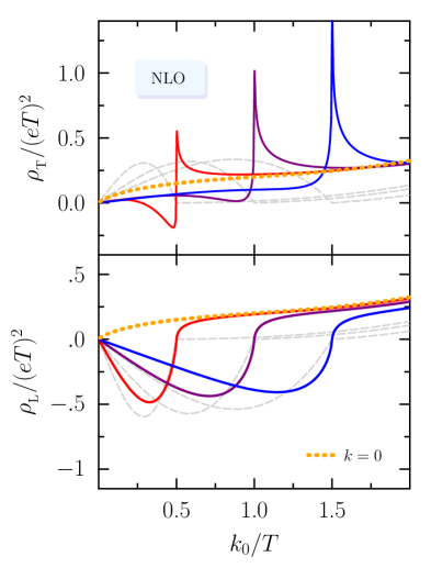
Figure 15: Transverse (upper panel) and longitudinal (lower panel) spectral functions for $k/T=0.5,1,1.5$ . Since $\rho_{{}_{\rm T}}=\rho_{{}_{\rm L}}$ for a photon at rest, the curves with $k=0$ are identical. As defined in Eq. (1.1), $e^{2}$ was factored out and we used a fixed strong coupling $g=3$ for illustration. The thin dashed lines are the LO result (i. e. $g=0$).

In heavy-ion collisions McLerran1985 ; Weldon1990iw , the observable photon and dilepton rates are proportional to $-\hbox{Im}\,\Pi^{\mu}_{\ \mu}=2\rho_{{}_{\rm T}}+\rho_{{}_{\rm L}}$ for $K^{2}=0$ and $K^{2}\geq 4m^{2}_{l}$ respectively ($m_{l}$ is the lepton’s mass), where perturbative studies have hitherto focused. The complementary region, $K^{2}<0\,$, is not merely academic: It provides an opportunity to cross-check the weak coupling framework, e. g. with non-perturbative Euclidean correlators (of either polarisation) provided by lattice QCD Brandt2017 .

As noted in the Introduction, our results are relevant for deploying (fixed-order) perturbation theory in contexts where simplifying kinematic assumptions are not justified. It is nevertheless worthwhile, e. g. if analytic expressions are available, to check that these numerical results reproduce the correct behaviour in those limits. We have done this using the OPEs in Appendix D for $K^{2}\gg T^{2}$ in each integral studied. Our results are also compatible with recent HTL self-energies at NLO, in the limit $k_{0},\,k\ll T$ Carignano2019 .

It is worth recalling that the individual masters are not (usually) themselves physical, rather they supply a convenient ‘basis’ from which observables can be built. That ubiquity makes a dedicated study constructive because of the valuable resource it provides for future NLO developments at finite-$T\,$. Although by no means all-inclusive, the list of loop integrals compiled here should satisfy a wide variety of needs or take little generalising to do so.

Appendix A Thermal Phase Space

In this appendix, we discuss two important phase space integrals which were used in the main text. The following results are valid both above and below the lightcone: $k_{0}\mathrel{\hbox to0.0pt{\lower 2.5pt\hbox{$>$}\hss}\raise 2.5pt\hbox{$<$}}|\text{\boldmath$k$}|\,$. Without loss of generality, we assume $k_{0}$ is positive. Energy conservation is imposed by cutting the diagram, handled with the replacement

$$\hbox{Im}\,\frac{1}{k_{0}+i0^{+}-A}\,\to\,-\pi\delta(k_{0}-A)\,.$$

A.1 Two-particle decay

The production rate due to binary encounters, e.g. $q\bar{q}\to\gamma^{*}$ (the asterisk indicates a virtual photon), is given by a phase-space integration over the momenta of interacting partons. For a given external momentum $K=(k_{0},\text{\boldmath$k$})$, we simplify the integration measure

$$\int_{[1,2]} \equiv \sum_{v}\int_{\text{\boldmath$p$},\text{\boldmath$q$}}\frac{(2\pi)^{d+1}}{4E_{1}E_{2}}\delta^{(d+1)}(K-v_{1}P-v_{2}Q)\,,$$ (A.1)

with the (on-shell) energies $E_{1}=|\text{\boldmath$p$}|$, $E_{2}=|\text{\boldmath$q$}|$ . The $v_{i}=\pm 1$ are summed over, for $i=\{1,2\}$, so that in (A.1) each channel is represented. Here we also used dimensional regularisation for the terms ${\cal O}(\epsilon)$ needed later. Integrating over $d^{d}\text{\boldmath$q$}$ is trivial; momentum conservation fixes $\text{\boldmath$q$}=v_{2}(\text{\boldmath$k$}-v_{1}\text{\boldmath$p$})$ . The on-shell energy is therefore

$$E_{2} = |\text{\boldmath$k$}-v_{1}\text{\boldmath$p$}|\ =\ \sqrt{k^{2}+p^{2}-2v_{1}p\,k\,\cos\theta_{kp}}\,,$$ (A.2)

where $\theta_{kp}$ is the angle between $k$ and $p$ .

The external vector $k$ distinguishes an orientation with which to organise the remaining $d^{d}\text{\boldmath$p$}$-integration. We choose to align the $p_{z}$ axis with $k$, so that the azimuthal integration is also trivial. And instead of a polar integration over $\theta_{kp}$, we integrate over the magnitude $q=E_{2}$ given by (A.2). The angular limits accordingly translate into a kinematic restriction; $|k-v_{1}p|<q<|k+v_{1}p|$ (see Fig. 16). Let us therefore express the angular integration by

$$\bar{\mu}^{2\epsilon}\int\displaylimits_{0}^{\infty}\!\!dp\,p^{2-2\epsilon}\int\displaylimits_{0}^{\pi}\!\!d\theta_{kp}\ \sin^{1-2\epsilon}\theta_{kp} = \int\displaylimits_{0}^{\infty}\!\!dp\int\displaylimits_{|k-v_{1}p|}^{|k+v_{1}p|}\!\!dq\,\frac{pq}{k}\Big{(}\frac{4k^{2}\,\bar{\mu}^{2}}{4p^{2}q^{2}-(k^{2}-p^{2}-q^{2})^{2}}\Big{)}^{\epsilon}\,.$$

All the necessary scalar products can be formed in terms of these variables.

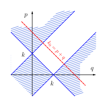
Figure 16: Allowable integration region in (A.1), where $p=v_{1}E_{1}$ and $q=v_{2}E_{2}$. The dashed line is the energy constraint $k_{0}=p+q$, while the blue shading is forbidden by the on-shell condition for $P$ and $Q=K-P$. (Here $K^{2}>0$.)

The combination $v_{1}p$ and $v_{2}q$ appears repeatedly above, suggesting that we formally extend the magnitudes $p$ and $q$ to negative values in lieu of summing over $\{v_{i}\}\,$. Thus the subsequent $(p,q)$-integration covers all channels, see Fig. 16, and reads

$$\sum_{v}\int\!\!dp\,dq = \int_{-\infty}^{+\infty}\!dp\,\Big{[}\,\int_{-|k+p|}^{-|k-p|}\!dq+\int_{|k-p|}^{|k+p|}\!dq\,\Big{]}\,.$$ (A.3)

When the internal lines are on-shell, energy conservation implies that $k_{0}=p+q$ allowing the $q$ integration in (A.3) to be carried out. Therefore the final result is supported only along dashed line shown in Fig. 16, and reads

$$\int_{[1,2]} = \frac{1}{8\pi\,k}\int^{\prime}\!\!\!dp\,\Big{(}\,1+\epsilon\log\frac{\bar{\mu}^{2}\,k^{2}}{K^{2}(p-k_{-})(p-k_{+})}+{\cal O}(\epsilon^{2})\,\Big{)}\,.$$ (A.4)

The $p$-integral was flagged with a prime as it depends on whether $K^{2}$ is positive or negative. In the former case (with $k_{0}>0$), only the channel having $v_{1}=v_{2}=+1$ contributes in (A.3). Precisely one of $v_{1}$ and $v_{2}$ equals $-1$ in the latter case.

Altogether, one has

$$\int^{\prime}\!\!dp \equiv \Theta(k_{-})\int_{k_{-}}^{k_{+}}\!\!dp-\Theta(-k_{-})\Big{[}\ \int_{-\infty}^{k_{-}}\!\!dp+\int_{k_{+}}^{\infty}\!\!dp\ \Big{]}\,.$$ (A.5)

The discontinuity at $k_{0}=k$ is thus given by an integral over all real $p\,$, in the principal valued sense. In the rest frame, $\text{\boldmath$k$}=0\,$, (A.4) has the net effect of setting $p=k_{0}/2$ .

As an application of the foregoing discussion, define

$$\psi_{s_{1},s_{2}}^{(\nu)} = \frac{n_{s_{0}}^{-1}}{k}\int^{\prime}\!\!dp\,n_{s_{1}}(p)n_{s_{2}}(k_{0}-p)\Big{(}\frac{p}{k_{0}}\Big{)}^{\nu}\ ,$$

and consider it for $\nu=\{0,1,2\}$ in particular. This function, which is needed for the one-loop discontinuity, was also used in the virtual parts of our two-loop calculations.

Letting the exponentials be abbreviated by

$${\cal E}_{\pm}\equiv\exp[\,-\beta|k_{\pm}|\,]\,,$$

we find that

$$\psi_{s_{1},s_{2}}^{(0)} = \Theta(k_{-})\ +\ \frac{T}{k}\log\frac{(1-s_{1}{\cal E}_{+})(1-s_{2}{\cal E}_{+})}{(1-s_{1}{\cal E}_{-})(1-s_{2}{\cal E}_{-})}\ ,$$ (A.7)

$$\psi_{s_{1},s_{2}}^{(1)} = \frac{1}{2}\Theta(k_{-})\ +\ \frac{T}{kk_{0}}\,\bigg{[}\ k_{0}\log\frac{1-s_{2}{\cal E}_{+}}{1-s_{2}{\cal E}_{-}}+k_{+}\log\frac{1-s_{1}{\cal E}_{+}}{1-s_{2}{\cal E}_{+}}-k_{-}\log\frac{1-s_{1}{\cal E}_{-}}{1-s_{2}{\cal E}_{-}}$$

$$\ -\ T\Big{(}\,\hbox{Li}_{2}(s_{1}{\cal E}_{+})+\hbox{sgn}(k_{-})\hbox{Li}_{2}(s_{1}{\cal E}_{-})-\hbox{Li}_{2}(s_{2}{\cal E}_{+})-\hbox{sgn}(k_{-})\hbox{Li}_{2}(s_{2}{\cal E}_{-})\,\Big{)}\ \bigg{]}\ ,$$

$$\psi_{s_{1},s_{2}}^{(2)} = \frac{1}{4k_{0}^{2}}\Big{(}\,k_{0}^{2}+\frac{k^{2}}{3}\,\Big{)}\Theta(k_{-})\ +\ \frac{T}{kk_{0}^{2}}\,\bigg{[}\ k_{+}^{2}\log\frac{1-s_{1}{\cal E}_{+}}{1-s_{2}{\cal E}_{-}}-k_{-}^{2}\log\frac{1-s_{1}{\cal E}_{-}}{1-s_{2}{\cal E}_{+}}$$ (A.9)

$$\ -\ 2Tk_{+}\Big{(}\,\hbox{Li}_{2}(s_{1}{\cal E}_{+})+\hbox{sgn}(k_{-})\hbox{Li}_{2}(s_{2}{\cal E}_{-})\,\Big{)}+2Tk_{-}\Big{(}\,\hbox{Li}_{2}(s_{2}{\cal E}_{+})+\hbox{sgn}(k_{-})\hbox{Li}_{2}(s_{1}{\cal E}_{-})\,\Big{)}$$

$$\ -\ 2T^{2}\Big{(}\,\hbox{Li}_{3}(s_{1}{\cal E}_{+})-\hbox{Li}_{3}(s_{1}{\cal E}_{-})+\hbox{Li}_{3}(s_{2}{\cal E}_{+})-\hbox{Li}_{3}(s_{2}{\cal E}_{-})\,\Big{)}\ \bigg{]}\ .$$

These quantities are discontinuous on the light cone, explicitly with

ψ(ν)s1,s2|k0=k+0+−ψ(ν)s1,s2|k0=k−0+112+2T2k2(Li2(s1)−Li2(s2))13−4T2k2Li2(s2).fragments fragmentsψ𝜈subscript𝑠1subscript𝑠2|subscript𝑘0𝑘superscript0ψ𝜈subscript𝑠1subscript𝑠2|subscript𝑘0𝑘superscript01fragments122superscript𝑇2superscript𝑘2(Li2(s1)Li2(s2))fragments134superscript𝑇2superscript𝑘2Li2(s2)\displaystyle\begin{tabular}[]{c || c | c | c }$\nu$&$0$&$1$&$2$\\ \hline\cr&&&\\[-11.38109pt] $\displaystyle\psi^{(\nu)}_{s_{1},s_{2}}\big{|}_{k_{0}=k+0^{+}}-\psi^{(\nu)}_{s_{1},s_{2}}\big{|}_{k_{0}=k-0^{+}}$&$1$&$\displaystyle\frac{1}{2}+2\frac{T^{2}}{k^{2}}\big{(}\hbox{Li}_{2}(s_{1})-\hbox{Li}_{2}(s_{2})\big{)}$&$\displaystyle\frac{1}{3}-4\frac{T^{2}}{k^{2}}\hbox{Li}_{2}(s_{2})$\\[5.69054pt] \end{tabular}\ .

ν012ν012

A.2 Three-particle decay

It is sufficient to work in $d=3$ dimensions for phase space integrations of the real two-loop corrections (those where three propagating particles are put on-shell). Extending (A.1), we define

$$\int_{[1,2,3]} \equiv \sum_{v}\int_{\text{\boldmath$p$},\text{\boldmath$q$},\text{\boldmath$r$}}\frac{(2\pi)^{4}}{8E_{1}E_{2}E_{3}}\delta^{(4)}(K-v_{1}P-v_{2}Q-v_{3}R)\,,$$ (A.11)

with the (on-shell) energies $E_{1}=|\text{\boldmath$p$}|$, $E_{2}=|\text{\boldmath$q$}|$ and $E_{3}=\sqrt{\text{\boldmath$r$}^{2}+\lambda^{2}}$. (The regulator $\lambda$ is necessary to observe the cancelling divergence between real and virtual corrections.) The $v_{i}=\pm 1$ are summed over, for $i=\{1,2,3\}$ . One of the integrals may be simplified using energy and momentum conservation; we choose the $r$-integral, and complete it by writing

$$\int_{\text{\boldmath$r$}}\frac{1}{2E_{3}} = 2\pi\int_{\text{\boldmath$r$}}\int_{-\infty}^{+\infty}\!\frac{dr_{0}}{2\pi}\delta(R^{2}-\lambda^{2})\Theta(r_{0})\,.$$

Hence, by fixing $\underline{R}=v_{3}(K-v_{1}P-v_{2}Q)$, we are left with

$$\int_{[1,2,3]} = 2\pi\sum_{v}\int_{\text{\boldmath$p$},\text{\boldmath$q$}}\frac{v_{3}}{4E_{1}E_{2}}\,\Theta(\underline{r}_{0})\delta\big{(}\underline{R}^{2}-\lambda^{2}\big{)}\,.$$ (A.12)

Let us now specify a coordinate system in order to proceed. We choose, following Ref. Peigne2007 , to align the $z$-axis along the direction of $k$ and orient the $zy$-plane to contain $p$, viz.

$$k = k(0,0,1)\,,$$

$$p = p(0,\sin\theta_{1},\cos\theta_{1})\,,$$

$$q = q(\sin\theta_{2}\sin\phi,\sin\theta_{2}\cos\phi,\cos\theta_{2})\,.$$ (A.13)

The integral over the azimuthal angle $\phi$ can then be performed in (A.12). To do so, express the argument of the $\delta$-function by $\underline{R}^{2}-\lambda^{2}=A+B\cos\phi$, where

$$A = K^{2}-\lambda^{2}+2\big{[}v_{1}p\,v_{2}q(1-x_{1}x_{2})-v_{1}p(k_{0}-x_{1}k)-v_{2}q(k_{0}-x_{2}k)\big{]}\,,$$

$$B = -2\Big{(}\,v_{1}p\sqrt{1-x_{1}^{2}}\,\Big{)}\Big{(}\,v_{2}q\sqrt{1-x_{2}^{2}}\,\Big{)}\,.$$ (A.14)

Here we have abbreviated $x_{i}=\cos\theta_{i}\,$. Consider then the integral of a function $g(\phi)\,$,

$$\int_{0}^{2\pi}\!d\phi\ \delta\big{(}\underline{R}^{2}-\lambda^{2}\big{)}\,g(\phi)=\frac{\Theta(h)}{\sqrt{h}}\sum_{\pm}g(\phi_{\pm})\,,$$

where $h=B^{2}-A^{2}$ and the angles $\phi_{\pm}=\pi\pm{\rm acos}(A/B)$. For our purposes, the function $g$ depends on $\phi$ via $\cos\phi$ and hence $\sum_{\pm}g(\phi_{\pm})\to 2g(\phi_{\pm})$ .

We have accomplished five of the nine integrals in (A.11), and are left with

$$\int_{[1,2,3]} = \frac{1}{4(2\pi)^{4}}\sum_{v}\int\!\!dp\,dx_{1}\int\!\!dq\,dx_{2}\hbox{sgn}(k_{0}-p-q)\,pq\frac{\Theta(h)}{\sqrt{h}}\,,$$ (A.15)

which cannot be simplified further in general. The combination $v_{1}p$ and $v_{2}q$ in (A.14) once again suggests that we formally extend the magnitudes $p$ and $q$ to negative values. The factor of $\Theta(\underline{r}_{0})$ in (A.12) has been dropped because $\underline{r}_{0}=v_{3}(k_{0}-v_{1}p-v_{3}q)$ and so exactly one term in the sum over $v_{3}=\pm 1$ will contribute. (The relevant value for $v_{3}$ is determined for a given $p$ and $q$ – extended to take negative values.) And then, as before, we can just forget the sum over $\{v_{i}\}$.

The $h$-function of (A.15) is quadratic in each of its arguments $p$, $x_{1}$, $q$, and $x_{2}$. Requiring $h\geq 0$ (equivalent to taking the real part of $\sqrt{h}$) summarises the allowable phase space.

Appendix B One-loop Auxiliary Functions

B.1 $F_{m}$ for $m=0,1,2$

The formula for $F_{0}$ was already given in the main text: see (3.4). Here we derive that result after discussing some simple properties. The expansion of the function $F_{0}$ about the light cone energy, $k_{0}=k\,$, is

$$F_{0}(K;s_{1},s_{2}) = \frac{-1}{32\pi k(k_{0}-k)}\bigg{[}\,T\frac{1+s_{2}}{(k_{0}-k)}+\big{(}\,\tfrac{1}{2}+s_{1}n_{s_{1}}(k)\,\big{)}\,+\,{\cal O}(k_{0}-k)\,\bigg{]}\,.$$ (B.1)

Whether the leading term has a double-pole depends upon $s_{2}=+1\,$, implying the propagator that appears twice is bosonic. If rather $s_{2}=-1\,$, then the pole is only simple. Equation (3.4) includes the vacuum result $-1/(16\pi K^{2})\,$, which we subtract in Fig. 17. Therefore the vertical intercept (at $k_{0}=0$) in this figure is merely $k^{2}/T^{2}\,$.

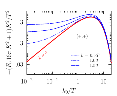
Figure 17: The thermal part (i.e. we subtracted the $T\to 0$ limit) of the function $F_{0}(K;+,+)$, for several values of the three momentum. The continuity in the function at $k_{0}=k$ for $k>0$ is an aspect of the repeated pole in (B.1).

A mass regulator $\lambda$ helps to evaluate $F_{0}\,$, by writing the repeated propagator as

$$\Delta^{2}_{s_{2}}(L)\ =\ \partial_{\lambda^{2}}\text{\boldmath$($}\Delta_{s_{2}}(L_{\lambda})\text{\boldmath$)$}\big{|}_{\lambda\to 0}\,,$$

where $L_{\lambda}=(\ell_{0},\,\text{\boldmath$\ell$}_{\lambda})$ is a four momentum with $|\text{\boldmath$\ell$}_{\lambda}|=\sqrt{\ell^{2}+\lambda^{2}}\,$. This calls for the one-loop results, provided in Appendix A, to be endowed with a mass on one of the propagators.

The integration methods are only slightly modified by the presence of a mass term above. On-shell energies are then $E_{1}=|\text{\boldmath$p$}|$ and $E_{2}=|\text{\boldmath$\ell$}_{\lambda}|\,$, and the integration limits are determined by energy conservation. We find, by generalising definition (A.1) to massive particles,

$$\hbox{Im}\,{\hbox{$\textstyle\sum$}\!\!\!\!\!\!\!\int\,}_{\!\!\!\!\raise-1.50694pt\hbox{$\scriptstyle{\,L}$}}\Delta_{s_{1}}(K-L)\Delta_{s_{2}}(L_{\lambda}) = \!-\int_{[1,2]}\big{(}f_{s_{1}}^{v_{1}}f_{s_{2}}^{v_{2}}-f_{s_{1}}^{-v_{1}}f_{s_{2}}^{-v_{2}}\big{)}$$

$$= \!-\frac{n_{s_{0}}^{-1}}{8\pi k}\int\!\!dp\,d\ell\frac{p\,\ell}{E_{1}E_{2}}\delta(k_{0}-e_{1}-e_{2})\,n_{s_{1}}(e_{1})n_{s_{2}}(e_{2})\,.$$

The signed energies introduced are $e_{1}=\hbox{sgn}(p)E_{1}$ and $e_{2}=\hbox{sgn}(q)E_{2}\,$. It is necessary to take the derivative of (B.1) with respect to $\lambda^{2}$ (and evaluate it at $\lambda=0$). For this purpose the integration variables are changed to $e_{1}$ and $e_{2}$ so that $\lambda$-dependence is swept into the limits of integration. The $\delta$-function then imposes the following limits on the $p$-integration:

$$\left\{\begin{array}[]{l}\displaystyle p>k_{-}+\frac{\lambda^{2}}{4k_{-}}\quad{\rm and}\quad p<k_{+}+\frac{\lambda^{2}}{4k_{+}}\\[11.38092pt] \displaystyle p<k_{-}+\frac{\lambda^{2}}{4k_{-}}\quad\ {\rm or}\ \quad p>k_{+}+\frac{\lambda^{2}}{4k_{+}}\\ \end{array}\right.\quad{\rm for}\quad k\mathrel{\hbox to0.0pt{\lower 2.5pt\hbox{$>$}\hss}\raise 2.5pt\hbox{$<$}}k_{0}\,.$$ (B.5)

We only need to evaluate the integrand at the appropriate boundary values (with $\lambda=0$), to obtain $F\,$. The result is stated in Eq. (3.4), in a way that is valid for either sign of $K^{2}$.

Using the approach stated in Sec. 2.1 to include powers of $p_{0}$ into the above derivation, one obtains expressions for $F_{1}$ and $F_{2}\,$. Casting them altogether gives (3.4). The resulting functions are plotted in Fig. 18, omitting the large-$k_{0}$ behaviour of (3.4), namely [see also Eq. (D.9)]

$$F_{0}=-1/(16\pi\,K^{2})\,,\qquad F_{1}=-k_{0}/(16\pi\,K^{2})\,,$$

$$F_{2}=-3k_{0}^{2}/(64\pi\,K^{2})\ ;\quad k_{0}\to\infty\,.$$

We note that in this limit, the coefficient of the $T^{2}$ thermal contribution is zero. (Which is also the case for the statistical combinations not plotted.)

Some relations can be derived for these functions. For the special case that $s_{1}=s_{2}\,$, one has $F_{1}=k_{0}\,F_{0}\,$. In general, $F_{2}$ is actually expressible by $F_{1}$ and $F_{0}$ due to the identity:

$$K^{2}\,F_{0}-4(k_{0}\,F_{1}-F_{2})=0\,,$$

which can be used in (3.3) for the first of the two master integrals when $m=2\,$.

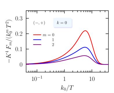
Figure 18: The energy dependence of the family of functions $F_{m}$ for $m=\{0,1,2\}$ at $k=0\,$. We show here the functions for $s_{1}=-1$ and $s_{2}=+1\,$, with their $k_{0}\to\infty$ limits subtracted out. The $m=0$ curve was also shown in Fig. 17.

B.2 $H_{m}$ and its ${\cal O}(\epsilon)$ contribution

In this section, we explain the functions $H_{m}^{[0,1]}$ as defined by Eq. (3.7) of the main text. To first establish $H_{m}$ from (3.5), it can be written as

$$H_{m}(K;s_{1},s_{2}) = -\int_{[1,2]}\big{(}f_{s_{1}}^{v_{1}}f_{s_{2}}^{v_{2}}-f_{s_{1}}^{-v_{1}}f_{s_{2}}^{-v_{2}}\big{)}(v_{1}E_{1})^{m}\,,$$ (B.6)

for $m=0,1,2$ with the special notation of Appendix A.1. In the special case that $s_{1}=s_{2}\,$, one may show that $H_{1}=\tfrac{1}{2}k_{0}H_{0}$ by a change of integration variables. But in general, one must adhere to (A.4) for the integration. According to that formulation we can set $v_{1}=v_{2}=+1$ enabling the distribution functions to be written

$$f_{s_{1}}^{+}f_{s_{2}}^{+}-f_{s_{1}}^{-}f_{s_{2}}^{-}\ =\ \text{\boldmath$($}e^{k_{0}/T}-s_{1}s_{2}\text{\boldmath$)$}\,n_{s_{1}}n_{s_{2}}\ ,$$

where the arguments were omitted.

The results are immediate: [The primed integral is defined in (A.5).]

$$H_{m}^{[0]} = k_{0}^{m}\,\psi^{(m)}_{s_{1},s_{2}}\ ,$$ (B.7)

$$H_{m}^{[1]} = \frac{n_{0}^{-1}}{k}\int^{\prime}\!\!dp\ p^{m}\,n_{1}n_{2}\log\frac{k^{2}}{(p-k_{-})(p-k_{+})}\ .$$

B.3 Finite part of $G_{m}$

We now consider $G_{m}^{[0]}$, defined in Eq. (3.7) of the main text, for $m=\{0,1\}$.

The whole function $G_{0}$ is equal to the real part of

$$-\sum_{v}\int_{\text{\boldmath$p$}}\frac{1}{4E_{1}E_{2}}\frac{v_{1}(\tfrac{1}{2}+s_{2}n_{s_{2}}(E_{2}))+v_{2}(\tfrac{1}{2}+s_{1}n_{s_{1}}(E_{1}))}{k_{0}-v_{1}E_{1}-v_{2}E_{2}}\ .$$

In the sum above, where $v_{1}=v_{2}$ the ‘$\tfrac{1}{2}$’-terms combine into what becomes the vacuum result. Anything proportional to the distribution functions gives thermal effects, and we use a symmetry to write $n_{s_{2}}$ with the argument $E_{1}\,$. Making use of (A.3), without imposing the energy constraint, it is necessary to also add the contribution coming from ${k_{0}\to-k_{0}}\,$. We can complete all but one of the integrations to obtain

$$G_{0}^{[0]}(K;s_{1},s_{2}) = \frac{1}{k}\int_{0}^{\infty}\!dp\big{(}s_{1}n_{s_{1}}(p)+s_{2}n_{s_{2}}(p)\big{)}\Gamma_{0}(p,k_{0},k)\ ,$$

$$\Gamma_{0}(p,k_{0},k) \equiv \log\frac{(k_{+}+p)(k_{-}-p)}{(k_{+}-p)(k_{-}+p)}\,.$$ (B.8)

For small $p$ relative to the external momentum, $\Gamma_{0}\simeq-8p\,k/K^{2}\,$ and therefore the integral is finite even if one of the distribution functions is bosonic. We have decided to work with all logarithms taking the absolute values of their arguments, but if we were careful to keep the correct sign one could use the imaginary part of (B.8) to determine $H_{0}\,$.

The function $G_{1}^{[0]}$ reads

$$G_{1}^{[0]}(K;s_{1},s_{2}) = \frac{k_{0}}{k}\int_{0}^{\infty}\!\!dp\,\Big{\{}\,s_{2}n_{s_{2}}(p)\Gamma_{0}(p,k_{0},k)+\big{(}s_{1}n_{s_{1}}(p)-s_{2}n_{s_{2}}(p)\big{)}\Gamma_{1}(p,k_{0},k)\,\Big{\}}\ ,$$

$$\Gamma_{1}(p,k_{0},k) \equiv \frac{p}{k_{0}}\log\frac{k_{+}^{2}(k_{-}^{2}-p^{2})}{k_{-}^{2}(k_{+}^{2}-p^{2})}\,,$$ (B.9)

and $\Gamma_{0}$ is as before, see (B.8). We note that $G^{[0]}_{1}=\tfrac{1}{2}G^{[0]}_{0}$ if $s_{1}=s_{2}\,$, as can be derived from the integral expression for $G_{1}\,$.

Appendix C Two-loop Kernels

In the diagrams labelled IV, V and VI, index $c$ is nonzero and therefore the momenta running in the loop do not decouple. After carrying out the sums over $p_{0}$ and $q_{0}$ in (2.1), following e. g. Ref. BP , the terms can be sensibly collected according to which energies are on-shell. The main virtue of our strategy for $m,n\geq 0$ (discussed in Sec. 2) is that it means we can perform the frequency sums assuming $m=n=0\,$.

For IV, the outcome is (4) with all intermediate particles on-shell. That is generally the form the ‘real’ corrections will take. Having more propagators (via $d,e\neq 0$) will facilitate other permutations of cuts. The type-V master integral has more, which are represented by the two terms in the following expression for the imaginary part:

$$\hbox{Im}\ {\cal I}_{11110}^{(0)}\! = \int_{[1,4]}\big{(}\,f_{s_{1}}^{v_{1}}f_{s_{4}}^{v_{4}}-f_{s_{1}}^{-v_{1}}f_{s_{4}}^{-v_{4}}\,\big{)}$$

$$\times \Big{\{}\,\sum_{v_{2}}\int_{\text{\boldmath$q$}}\frac{\frac{1}{2}+s_{2}n_{2}(E_{2})}{2E_{2}(R^{2}-\lambda^{2})}\,+\sum_{v_{3}}\int_{\text{\boldmath$r$}}\frac{\frac{1}{2}+s_{3}n_{3}(E_{3})}{2E_{3}(v_{4}L-v_{3}R)^{2}}\,\Big{\}}$$

$$- \int_{[1,2,3]}\frac{f_{s_{1}}^{v_{1}}f_{s_{2}}^{v_{2}}f_{s_{3}}^{v_{3}}-f_{s_{1}}^{-v_{1}}f_{s_{2}}^{-v_{2}}f_{s_{3}}^{-v_{3}}\ }{(K-v_{1}P)^{2}}\ .$$

(The notation of the outermost integrals was defined in Appendix A.) Three momenta are put on-shell in the third line, now with an internal propagator that was not needed before. The virtual correction [equal to the part of (C)] has factored into a binary decay amplitude multiplying a one-loop vertex amplitude. Note that the ‘mass’ $\lambda^{2}$ has been introduced as a regulator, so that $R$ has on-shell energy $E_{3}=\sqrt{r^{2}+\lambda^{2}}$. Later we will take the limit $\lambda\to 0$ and find that the real and virtual pieces dovetail together, leaving a result that is both finite and $\lambda$-independent. The other energies are as before: $E_{1}=|\text{\boldmath$p$}|$ and $E_{2}=|\text{\boldmath$q$}|$, and we also denoted $L=K-v_{1}P$ and $R=K-v_{1}P-v_{2}Q$.

The imaginary part of the special integral in (5) is given explicitly by

$$\!\!\!\!\!\!\hbox{Im}\ {\cal I}_{11110}^{\text{\,\large$\star$}}=\int_{[1,4]}\big{(}\,f_{s_{1}}^{v_{1}}f_{s_{4}}^{v_{4}}-f_{s_{1}}^{-v_{1}}f_{s_{4}}^{-v_{4}}\,\big{)}$$

$$\times \bigg{\{}\,\sum_{v_{2}}\int_{\text{\boldmath$q$}}\frac{\frac{1}{2}+s_{2}n_{2}(E_{2})}{2E_{2}(R^{2}-\lambda^{2})}(2v_{2}\,K\cdot Q)\,+\sum_{v_{3}}\int_{\text{\boldmath$r$}}\frac{\frac{1}{2}+s_{3}n_{3}(E_{3})}{2E_{3}(v_{4}L-v_{3}R)^{2}}(2v_{4}\,K\cdot L-2v_{3}\,K\cdot R)\,\bigg{\}}$$

$$- \int_{[1,2,3]}\big{(}\,f_{s_{1}}^{v_{1}}f_{s_{2}}^{v_{2}}f_{s_{3}}^{v_{3}}-f_{s_{1}}^{-v_{1}}f_{s_{2}}^{-v_{2}}f_{s_{3}}^{-v_{3}}\,\big{)}\frac{2v_{2}\,K\cdot Q}{(K-v_{1}P)^{2}}\,.$$

The most intricate two-loop topology, yet benefiting from the most symmetry, as four different cuts contribute to the discontinuity, given by the following expression:

Im $$\!\!\!\!\!\!\!\!\!\!{\cal I}^{(0)}_{11111}\,=\,\bigg{[}\int_{[1,4]}\big{(}\,f_{s_{1}}^{v_{1}}f_{s_{4}}^{v_{4}}-f_{s_{1}}^{-v_{1}}f_{s_{4}}^{-v_{4}}\,\big{)}$$

$$\times \bigg{\{}\,\sum_{v_{2}}\!\int_{\text{\boldmath$q$}}\frac{\frac{1}{2}+s_{2}n_{s_{2}}(E_{2})}{2E_{2}(R^{2}-\lambda^{2})V^{2}}+\sum_{v_{5}}\!\int_{\text{\boldmath$v$}}\frac{\frac{1}{2}+s_{5}n_{s_{5}}(E_{5})}{2E_{5}(R^{2}-\lambda^{2})Q^{2}}+\sum_{v_{3}}\!\int_{\text{\boldmath$r$}}\frac{\frac{1}{2}+s_{3}s_{s_{3}}(E_{3})}{2E_{3}Q^{2}V^{2}}\,\bigg{\}}$$

$$- \int_{[1,2,3]}\frac{f_{s_{1}}^{v_{1}}f_{s_{2}}^{v_{2}}f_{s_{3}}^{v_{3}}-f_{s_{1}}^{-v_{1}}f_{s_{2}}^{-v_{2}}f_{s_{3}}^{-v_{3}}\ }{(K-v_{1}P)^{2}(K-v_{2}Q)^{2}}\,\bigg{]}+\bigg{[}\quad s_{1}\leftrightarrow s_{5}\,,\ s_{2}\leftrightarrow s_{4}\quad\bigg{]}\ .$$

The meaning of the third line should be clear, the second line is one of the virtual corrections. It possess three terms which ought to be clarified. The momenta $P$ and $L=v_{4}(K-v_{1}P)$ are on-shell with $E_{1}=|\text{\boldmath$p$}|$ and $E_{4}=|\text{\boldmath$\ell$}|\,$. Inside the curly braces we have defined

$$R\ = v_{4}L-v_{2}Q\ =\ v_{5}V-v_{1}P\ ,$$

$$V\ = K-v_{2}Q\ =\ v_{3}R-v_{1}P\ ,$$

$$Q\ = K-v_{5}V\ =\ v_{4}L-v_{3}R\ ,$$ (C.4)

together with the energies $E_{2}=|\text{\boldmath$q$}|$, $E_{3}=\sqrt{\text{\boldmath$r$}^{2}+\lambda^{2}}$ and $E_{5}=|\text{\boldmath$v$}|\,$. (The necessary form to use should be clear from the $v$-sum and spatial integrals.)

C.1 Real corrections, $W(p,q)$

Here we derive the expression given in (4), by explicitly carrying out the angular integrals from (4). The result of Appendix A, and specifically Eq. (A.15), shows that we can identify

$$W_{\rm I\!V}(p,q) = \hbox{sgn}(k_{0}-p-q)\frac{pq}{\pi}\int\!dx_{2}\,dx_{1}\frac{\Theta(h)}{\sqrt{h}}\,.$$ (C.5)

The meaning of $h$ and the boundaries on the integrals were given there. One may safely set $\lambda=0$ (it does not generate the collinear logarithms), which simplifies the kinematical constraints from $h\geq 0$. Starting with the angular integration over $x_{1}=\cos\theta_{kp}$ in (A.15), we write the function $h=h(x_{1})$ as a quadratic: $ax_{1}^{2}+bx_{1}+c$ Peigne2007 . The coefficients, which can be calculated from (A.14), are

$$a\! = \!-4p^{2}(k^{2}+2kqx_{2}+q^{2})\ ,$$

$$b\! = \!4p(k-qx_{2})\big{[}k_{0}^{2}+k^{2}-2(k_{0}-p)(k_{0}-q)-2kqx_{2}\big{]}\,,$$

$$c\! = \!4p^{2}q^{2}(1-x_{2}^{2})-\big{(}K^{2}+2[pq-k_{0}p-q(k_{0}-kx_{2})]\big{)}^{2}\,.$$ (C.6)

Because $a<0\,$, the $\Theta$-function in (C.5) dictates the upper and lower limits on the $x_{1}$ integration. We can parametrise $x_{1}$ in terms of the ‘angle’ $\xi\in(0,\pi)$ with

$$x_{1}(\xi) = \frac{-b+\cos\xi\sqrt{\Delta}}{2a}\,,$$ (C.7)

where $\Delta=b^{2}-4ac$ is the discriminant. Changing the integration variable from $x_{1}$ to $\xi$ thus removes the $\Theta$-function and yields

$$\int_{-1}^{+1}\!dx_{1}\frac{\Theta(h)}{\sqrt{h}}F(x_{1}) = |a|^{-\nicefrac{{1}}{{2}}}\!\int_{0}^{\pi}\!d\xi F\text{\boldmath$($}x_{1}(\xi)\text{\boldmath$)$}\,.$$

It turns out that $\Delta\geq 0$ summarises the allowable phase space, which we have elaborated previously (in the momenta $p$ and $q$). We already assumed a permissible $(p,q)$ configuration by writing out the $x_{1}$-integral.

Returning to (C.5), this gives

$$W_{\rm I\!V}(p,q) = \hbox{sgn}\Big{(}p(k_{0}-p-q)\Big{)}\frac{q}{2}\int_{x_{2}^{\rm min}}^{x_{2}^{\rm max}}\!\!\frac{dx_{2}}{\sqrt{k^{2}-2kpx_{2}+p^{2}}}\,.$$ (C.8)

The limits above follow from requiring $\Delta\geq 0$ in (C.7), so that the integral has non-zero support. They are, for sanctioned $p$ and $q$ values,

$$x_{2}^{\rm max} = \,\min\Big{[}+1,\max\big{[}X,Y\big{]}\Big{]}\ ,$$

$$x_{2}^{\rm min} = \max\Big{[}-1,\,\min\big{[}X,Y\big{]}\Big{]}\ .$$ (C.9)

where

$$X=\frac{2k_{0}q-K^{2}}{2kq}\quad{\rm and}\quad Y=X+\frac{2}{kq}p(k_{0}-p-q)\,.$$

One may check that this reproduces the formula in (4).

The same approach works for calculating $W_{\rm V}$ and $W_{\rm VI}\,$, however $\lambda\neq 0$ must be kept wherever a log-divergence may occur. Determining $h$ and the limits $x_{2}^{\rm min}$ and $x_{2}^{\rm max}$ in each of the regions defined by Figs. 6 and 7 leads to the expressions (5.13) and (6).

Let us note that the angular limits in (C.9) apply to all the real two-loop contributions. Harking back to Figs. 6 and 7, these limits are specifiable in each region of the $(p,q)$-plane. Considering them individually reveals how for $k_{0}\simeq k\,$, the prima facie incompatible regions interchange when moving from above to below the light cone: If one takes the limit $k_{0}\to k+0^{+}$ (see Fig. 19), the $x_{2}$-limits coincide thus giving zero precisely where $p$ and $q$ are kinematically forbidden in the spacelike region. A similar argument works out for $k_{0}\to k-0^{+}\,$. Moreover, the angular limits are well-defined for $k_{0}=k$ in the nontrivial regions that remain (i.e. ‘2’, ‘3’ and ‘4’ from Fig 5). That implies the functions $W(p,q)$ that we calculate are continuous at $k_{0}=k\,$.

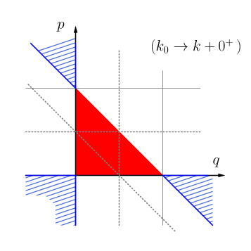
Figure 19: The allowable integration region in variables $p$ and $q\,$, as $k_{0}$ approaches $k$ from above. Region ‘1’ from Fig. 5 has been coloured (red) and is excluded by observing that the upper and lower limits in the $x_{2}$-integration coincide.

This does not preclude the final master integrals from being infinite on the light cone. However, for those that are, the singularity must be the same whether approached from above or below. Some of the master integrals are finite at $k_{0}=k\,$, others diverge either logarithmically or due to a pole.

C.2 Virtual corrections, $U_{\rm V}(p\,;\lambda)$

The two terms in the second line of (C) may be calculated by a standard Feynman parametrisation. Let us manipulate these terms assuming $v_{1}=v_{4}=+1$ (it does not lose any generality). We find

$$\sum_{v_{2}} \!\!\!\!\!\int_{\text{\boldmath$q$}}\frac{\frac{1}{2}+s_{2}n_{2}(E_{2})}{2E_{2}(R^{2}-\lambda^{2})}\,=\,\frac{1}{(4\pi)^{2}\ell}\int_{-\infty}^{+\infty}\!\!dq\big{(}\,\tfrac{1}{2}+s_{2}n_{s_{2}}(q)\,\big{)}\log\frac{\lambda^{2}}{4\ell q+\lambda^{2}}\,,$$ (C.10)

where $L=(\ell_{0},\text{\boldmath$\ell$})=K-P$ and $R=L-v_{2}Q\,$. (Here, as before, we absorb the sum over $v_{2}$ into the sign of $q$.) Similarly,

$$\sum_{v_{3}} \!\!\!\!\!\!\!\!\!\int_{\text{\boldmath$r$}}\frac{\frac{1}{2}+s_{3}n_{3}(E_{3})}{2E_{3}(L-v_{3}R)^{2}}\,=\,\frac{1}{(4\pi)^{2}\ell}$$

$$\times \int_{-\infty}^{+\infty}\!\!dr\frac{r}{e_{3}}\big{(}\,\tfrac{1}{2}+s_{3}n_{s_{3}}(e_{3})\,\big{)}\log\frac{\lambda^{2}-2\ell(e_{3}-r)}{\lambda^{2}-2\ell(e_{3}+r)}\,,$$

with a signed energy $e_{3}=\hbox{sgn}(r)\sqrt{\lambda^{2}+r^{2}}$. In this term, we change integration variables from $r$ to $q=k_{0}-p-e_{3}$ so that (C.2) and (C.10) are ready to be combined. But before doing that, a divergent contribution needs to be salvaged from this vertex correction. It is handily isolated (and underlined in what follows) by writing

$$\big{(}\,\tfrac{1}{2}+s_{2}n_{s_{2}}(q)\,\big{)}\ =\ \underline{\hbox{sgn}(q)\tfrac{1}{2}}+\hbox{sgn}(q)s_{2}n_{s_{2}}\big{(}|q|\big{)}\ .$$

in (C.10), and similarly a term like $\hbox{sgn}(r)\frac{1}{2}$ in (C.2). The other parts lead to momentum integrals that are rendered finite by the thermal weights. But the divergent vacuum result, using dimensional regularisation, is equal to

$$\int_{Q}\ \frac{1}{Q^{2}[(L-Q)^{2}-\lambda^{2}]} = \frac{1}{(4\pi)^{2}}\Big{(}\ \frac{1}{\epsilon}+\log\frac{\bar{\mu}^{2}}{\lambda^{2}}+1\ \Big{)}\,,$$

where $L^{2}=(K-P)^{2}=0$ was needed. This is what the curly braces in (C) produce in vacuum. With a large cut-off $\Lambda$ on the magnitude of $\text{\boldmath$q$}\,,$ it is easy to show how the same type of divergence arises. The restricted integral,

$$\int_{-\Lambda}^{+\Lambda}\frac{dq}{2}\,\Big{[}\,\hbox{sgn}(q)\log\frac{\lambda^{2}}{4\ell\,q}+\hbox{sgn}(\ell-q)\log\frac{\lambda^{2}q}{4\ell\,(\ell-q)^{2}}\,\Big{]}$$

$$=-\ell\,\Big{(}\,\log\frac{4\Lambda^{2}}{\lambda^{2}}+1+{\cal O}(\ell^{2}/\Lambda^{2})\,\Big{)}\,,$$

where we assumed $\lambda\to 0\,$. In this limit $e_{3}=r+\frac{\lambda^{2}}{2r}+\ldots$ , which enabled the arguments of the logarithms to be simplified. Hence using $\log 4\Lambda^{2}=\epsilon^{-1}+\log\bar{\mu}^{2}$ is the choice consistent with the two-point function in (LABEL:C2_-_6).

Returning to Eqs. (C.10) and (C.2), these two contributions can be drawn up against their real counterparts, by substituting

$$\big{(}\,\tfrac{1}{2}+s_{2}n_{s_{2}}\,\big{)}\ =\ -\big{(}\,\tfrac{1}{2}+s_{3}n_{s_{3}}\,\big{)}+\frac{n_{s_{2}}n_{s_{3}}}{n_{s_{4}}}\,,$$

where we identified $\ell=p+e_{3}$ and omitted arguments of the distribution functions. ($\ell$ is the argument of $n_{s_{4}}$ and $s_{4}=s_{0}\,s_{1}$.) For small $\lambda$, the expression in curly braces from (C) thus simplifies,

$$\lim_{\lambda\to 0}\big{\{}\ \cdots\ \big{\}} = \frac{1}{(4\pi)^{2}\ell}\int\!\!dq\ \Big{[}\ \frac{n_{s_{2}}n_{s_{3}}}{n_{s_{4}}}\log\frac{\lambda^{2}}{4\ell q}+\big{(}\,\tfrac{1}{2}+s_{3}n_{s_{3}}\,\big{)}\log\frac{q^{2}}{r^{2}}\ \Big{]}\,.$$ (C.13)

The first summand combines with the real corrections to remove any dependence on $\lambda$ overall. In the second, we again single out the divergent part and calculate it with a cut-off regulator. Namely, from

$$\int_{-\Lambda}^{+\Lambda}\!dq\ \hbox{sgn}(\ell-q)\log\frac{q^{2}}{(\ell-q)^{2}}=-2\ell\Big{(}\,\frac{1}{\epsilon}+\log\frac{\bar{\mu}^{2}}{4\ell^{2}}+2+{\cal O}(\ell^{2}/\Lambda^{2})\,\Big{)}\,,$$

which was converted to dimensional regularisation. Now ${\cal O}(\epsilon)$ terms in Eq. (A.4) must be kept for the outer integration. The sequestered part of (C.13) therefore generates

$$\frac{-1}{(4\pi)^{2}}\Big{[}\,\frac{1}{\epsilon}+2\log\frac{\bar{\mu}^{2}}{K^{2}}+\log\frac{K^{2}\,k^{2}}{4\ell^{2}(p-k_{-})(p-k_{+})}+2\,\Big{]}\,.$$ (C.14)

Equation (C.14) contains an ultraviolet divergence, which will end up being multiplied by a function of the temperature in the final expression. The first term in (C) can be written, after using signed momenta to incorporate the sum over the $\{v_{i}\}$,

$$\frac{1}{4(4\pi)^{3}\,k}\int^{\prime}\!dp\,\big{(}\,f_{s_{1}}^{+}f_{s_{4}}^{+}-f_{s_{1}}^{-}f_{s_{4}}^{-}\,\big{)}\big{\{}\ \cdots\ \big{\}}\ =\ \frac{n_{s_{0}}^{-1}}{(4\pi)^{3}}\int\!dp\,U^{(0)}_{\rm V}(p\,;\lambda)\,n_{s_{1}}n_{s_{4}}\,.$$

The formula for $U^{(0)}_{\rm V}$ was given in (5) of the main text.

Including an extra power of $q=v_{2}E_{2}$ [from $n=1$ in (5.3)] is a simple matter. None of the Feynman parametrisations or angular integrals are modified. The $\lambda$-singularities are also unchanged in (C.13), apart from an extra factor of $q\,$. The vacuum result

$$\int_{Q}\ \frac{q_{0}}{Q^{2}[(L-Q)^{2}-\lambda^{2}]} = \frac{\ell_{0}}{4(4\pi)^{2}}\Big{(}\ \frac{1}{\epsilon}+\log\frac{\bar{\mu}^{2}}{\lambda^{2}}+\frac{1}{2}\ \Big{)}\,,$$ (C.15)

must be recovered by our regularisation procedure. This can be checked by redoing the calculation with a cut-off, as before. But now one finds that $\log 4\Lambda^{2}=\epsilon^{-1}+\log\bar{\mu}^{2}+2$ is needed to consistently convert the restricted integral,

$$\int_{-\Lambda}^{+\Lambda}\!dq\ q\,\hbox{sgn}(\ell-q)\log\frac{q^{2}}{(\ell-q)^{2}}=-\ell^{2}\,\Big{(}\,\log\frac{\Lambda^{2}}{\ell^{2}}-1+{\cal O}(\ell^{2}/\Lambda^{2})\,\Big{)}\,,$$

to dimensional regularisation. The argument is otherwise unchanged, and altogether leads to the formula for $U^{(1)}_{\rm V}(p\,;\lambda)$ that was given in (5).

The special master integral, defined in (5), also follows along the lines above. Here we give some more details: The curly braces of Eq. (C) give, for $\lambda\to 0\,$,

$$\big{\{}\ \cdots\ \big{\}}\ =\ \frac{1}{(4\pi)^{2}\ell^{2}}\int\!dq\, \bigg{[} q\,\big{(}\,\tfrac{1}{2}+s_{2}n_{s_{2}}\,\big{)}\Big{(}\,2(K^{2}-2\ell k_{0})+K^{2}\log\frac{\lambda^{2}}{4\ell q}\,\Big{)}$$

$$- \!\!\big{(}\,\tfrac{1}{2}+s_{3}n_{s_{3}}\,\big{)}\Big{(}\,2r(K^{2}-2\ell k_{0})-qK^{2}\log\frac{\lambda^{2}q}{4\ell r^{2}}\,\Big{)}\ \bigg{]}\,.$$

Anything in the integrand that is proportional to a distribution function $n_{s_{2}}(|q|)$ or $n_{s_{3}}(|r|)$ (evaluated at positive arguments) will be finite. The divergent terms are easily isolated using the same approach as for $U_{\rm V}^{(0)}$ and $U_{\rm V}^{(1)}$. They can be calculated by a cut-off regulator, and altogether must give

$$\int_{Q}\ \frac{2\,K\cdot Q}{Q^{2}[(L-Q)^{2}-\lambda^{2}]} = \frac{-K^{2}}{2(4\pi)^{2}}\Big{(}\ \frac{1}{\epsilon}+\log\frac{\bar{\mu}^{2}}{\lambda^{2}}+\frac{1}{2}\ \Big{)}\,.$$

Once again, the hard cut-off integral can be given explicitly:

$$\int_{-\Lambda}^{+\Lambda}\!dq\,\Big{[}\,\hbox{sgn}(q)\Big{(}\,2q(K^{2}-2\ell k_{0})+qK^{2}\log\frac{\lambda^{2}}{4\ell q}\,\Big{)}$$

$$\qquad\quad-\,\hbox{sgn}(r)\Big{(}\,2r(K^{2}-2\ell k_{0})-qK^{2}\log\frac{\lambda^{2}q}{4\ell r^{2}}\,\Big{)}\,\Big{]}$$

$$=-\ell^{2}\,\Big{(}\,K^{2}\log\frac{4\Lambda^{2}}{\lambda^{2}}+\frac{1}{2}K^{2}-4k_{0}\ell+{\cal O}(\ell^{2}/\Lambda^{2})\,\Big{)}\,.$$

This part of (C.2) should give the complete vacuum result for the vertex correction and consequently, should be converted to dimensional regularisation using $\log 4\Lambda^{2}=\epsilon^{-1}+\log\bar{\mu}^{2}+4k_{0}\ell/K^{2}\,$. Going back to (C.2) and rearranging the distribution functions, the quantity in curly braces becomes, for $\lambda\to 0\,$,

$$\big{\{}\ \cdots\ \big{\}}\ =\ \frac{1}{(4\pi)^{2}\ell^{2}}\int\!dq \bigg{[} q\,\frac{n_{s_{2}}n_{s_{3}}}{n_{s_{4}}}\Big{(}\,2(K^{2}-2\ell k_{0})+K^{2}\log\frac{\lambda^{2}}{4\ell q}\,\Big{)}$$

$$+ \big{(}\,\tfrac{1}{2}+s_{3}n_{s_{3}}\,\big{)}\Big{(}\,-2\ell\,(K^{2}-2\ell k_{0})+qK^{2}\log\frac{q^{2}}{r^{2}}\,\Big{)}\ \bigg{]}\,.$$

The first line above will combine with the real corrections; cf. Eq. (5.13). A remnant, which is proportional to $\hbox{sgn}(r)\frac{1}{2}$ in the second line, diverges and can now be calculated with a regulator,

$$\int_{-\Lambda}^{+\Lambda}\! \displaystyle dq \!\hbox{sgn}(r)\,\Big{[}\,2\ell\,\Big{(}\,\frac{2\ell k_{0}}{K^{2}}-1\,\Big{)}+q\log\frac{q^{2}}{r^{2}}\,\Big{]}\ =\ -\ell^{2}\,\Big{(}\,\frac{1}{\epsilon}+\log\frac{\bar{\mu}^{2}}{4\ell^{2}}+3-\frac{4\ell k_{0}}{K^{2}}\,\Big{)}\,.$$

With that, inserted into (C.2), we are able to single out a fragment that is the same as $U_{\rm V}^{(1)}$ up to a factor of $K^{2}/\ell$. We thus arrive at Eq. (5.14) of the main text, after using the principal valued integral

$${\cal P}\!\int_{-\infty}^{+\infty}\!dq\ \hbox{sgn}(\ell-q)\,n_{s_{3}}(|\ell-q|)=0\,,$$

to drop some polynomial parts of the thermal proportion.

C.3 Virtual corrections, $U_{\rm VI}(p\,;\lambda)$

Moving along to the function $U_{\rm VI}^{(n)}(p\,;\lambda)$ needed in (6.2), we derive it from (C). Let us focus on the three terms in curly braces and consider them individually. The first, for $\lambda\to 0\,$, is

$$\sum_{v_{2}}\int_{\text{\boldmath$q$}}\frac{\text{\boldmath$($}\frac{1}{2}+s_{2}n_{s_{2}}(E_{2})\text{\boldmath$)$}\,q^{n}}{2E_{2}(R^{2}-\lambda^{2})V^{2}} = \frac{1}{(4\pi)^{2}K^{2}}\int_{-\infty}^{+\infty}\!\!\frac{dq\,q^{n}}{k_{0}-p-q}$$

$$\times \big{(}\,\tfrac{1}{2}+n_{2}\,\big{)}\log\frac{\lambda^{2}(k_{0}-p)(k_{-}-q)(k_{+}-q)}{K^{2}\,q(k_{0}-p-q)^{2}}\ .$$

To carry out the $v_{i}$-sums, the momenta $p$ and $q$ were extended to negative values. [Here only the $q$ integration is made plain, the impending outer $p$-integration takes the form of (A.4).] Similarly we find, for $\lambda\to 0\,$,

$$\sum_{v_{5}}\int_{\text{\boldmath$v$}}\frac{\text{\boldmath$($}\frac{1}{2}+s_{5}n_{s_{5}}(E_{5})\text{\boldmath$)$}q^{n}}{2E_{5}(R^{2}-\lambda^{2})Q^{2}} = \frac{1}{(4\pi)^{2}K^{2}}\int_{-\infty}^{+\infty}\!\frac{dv(k_{0}-v)^{n}}{v-p}$$

$$\times \big{(}\,\tfrac{1}{2}+n_{5}\,\big{)}\log\frac{K^{2}\,v(v-p)^{2}}{\lambda^{2}p(k_{-}-v)(k_{+}-v)}\ ,$$

where the integration variable $v$ has been extended to negative values. For the term where ‘particle-3’ is on-shell, we use the integration variable $r=v_{3}E_{3}$. Then, for $\lambda\to 0\,$,

$$\sum_{v_{3}}\int_{\text{\boldmath$r$}}\frac{\text{\boldmath$($}\frac{1}{2}+s_{3}s_{s_{3}}(E_{3})\text{\boldmath$)$}\,q^{n}}{2E_{3}\,Q^{2}\,V^{2}} = \frac{1}{(4\pi)^{2}K^{2}}\bigg{(}\!\int_{-\infty}^{-\lambda}\!dr+\!\int_{+\lambda}^{+\infty}\!dr\bigg{)}\ \frac{(\ell-r)^{n}}{r}$$

$$\times \!\!\big{(}\,\tfrac{1}{2}+n_{3}\,\big{)}\log\frac{\lambda^{4}\,p\,(k_{0}-p-r)\,(k_{0}-p)(r+p)}{K^{4}\,r^{4}}\ .$$

The restriction $E_{3}\geq\lambda$ assists to explicitly regulate the $r\approx 0$ singularity. Unlike in (C.3) and (C.3), where the corresponding integral may be understood in the principle valued sense, the risk that $s_{3}=+1$ in (C.3) would make this futile. Therefore we keep $\lambda$ to control the exclusion of this integration interval.

Let us change integration variables to $q=k_{0}-v$ instead of $v$ and $q=k_{0}-p-r$ instead of $r$ in (C.3) and (C.3) respectively. The distribution functions can be rewritten in a way that the singular terms coalesce with their real counterparts. We do this by using an identity to rewrite the integrand of (C.3),

$$\big{(}\tfrac{1}{2}+n_{3}\big{)}\log\frac{\lambda^{4}\,pq\ell v}{K^{4}\,r^{4}} = \Big{[}-\big{(}\tfrac{1}{2}+n_{2}\big{)}+\frac{n_{2}n_{3}}{n_{4}}\,\Big{]}\log\frac{\lambda^{2}\ell v}{K^{2}r^{2}}$$

$$+ \Big{[}+\big{(}\tfrac{1}{2}+n_{5}\big{)}-\frac{n_{3}n_{5}}{n_{1}}\,\Big{]}\log\frac{\lambda^{2}pq}{K^{2}r^{2}}\ .$$

The two lines above are related by the exchange $p\leftrightarrow\ell$ and $q\leftrightarrow v$ (together with same swap in statistics). Combining the result with (C.3) and (C.3) gives, for the curly braces in (C),

$$\big{\{}\,\cdots\,\big{\}}\ \to\ \frac{1}{(4\pi)^{2}K^{2}}\int\!\frac{dq\,q^{n}}{r}\!\! \Big{[} \big{(}\,n_{2}-n_{5}\,\big{)}\log\frac{(k_{-}-q)(k_{+}-q)}{qv}$$ (C.21)

$$+ \frac{n_{2}n_{3}}{n_{4}}\log\frac{\lambda^{2}\ell v}{K^{2}r^{2}}\ -\ \frac{n_{3}n_{5}}{n_{1}}\log\frac{\lambda^{2}pq}{K^{2}r^{2}}\ \Big{]}\,.$$

And therefore, taking into account the outer limits of integration [e.g. by using (A.4)], it is clear that (C.21) contributes to a subregion of the available $(p,q)$-plane in the real corrections. This is exactly where $o_{p}=1$ if $k_{0}>k$, and the dependence on $\lambda^{2}$ in the second line of (C.21) disappears when combined with the two real corrections in Eq. (6.2). (The same occurs if $k<k_{0}$, but then the cancellation happens when $\bar{o}_{p}=1$.) Note that the second term in the second line of (6.2) is to be included in the whole result.

The case $n=2$ needs to be handled with some care, as the subsequent $q$-integral diverges. [Equation (D) of Appendix D also exposes this fact.] That can be seen from the ultraviolet behaviour of the first line in (C.21), since for $q\to\pm\infty$ the difference $(n_{2}-n_{5})$ becomes $\pm 1\,$, and the logarithm

$$\log\frac{(k_{-}-q)(k_{+}-q)}{qv}\ \simeq\ \frac{K^{2}}{4q^{2}}\,\Big{[}\,1+\frac{k_{0}}{q}+\frac{7k_{0}^{2}+k^{2}}{8q^{2}}+\ldots\,\Big{]}\,.$$

Hence the integration in (C.21) will be log-divergent for $n=2\,$, due to the $1/r=1/(k_{0}-p-q)$ left over. It can be attributed to the vertex correction, i. e. the three-point function studied in Ref. PV . The entry of the rank-2 tensor that we need, is given by

$$\lim_{\lambda\to 0}\int_{Q}\ \frac{q_{0}^{2}}{Q^{2}\,V^{2}(R^{2}-\lambda^{2})} = \frac{1}{(4\pi)^{2}\,K^{2}}\Big{[}\,\frac{K^{2}}{4}\Big{(}\,\frac{1}{\epsilon}+4+\frac{k^{2}-6p\ell}{K^{2}}+\log\frac{\bar{\mu}^{2}}{K^{2}}\,\Big{)}$$

$$+ \big{(}\,\tfrac{3}{2}k_{0}^{2}-5k_{0}p+3p^{2}\,\big{)}\Big{(}\,1+\log\frac{\lambda^{2}}{K^{2}}\,\Big{)}\ -\ \frac{\ell^{2}}{2}\,\Big{(}\,\frac{\pi^{2}}{3}-\log^{2}\frac{\lambda^{2}}{K^{2}}\,\Big{)}\,\Big{]}\,.$$

The ‘$\tfrac{1}{2}$’-terms next to the distribution functions in Eqs. (C.3)-(C.3) concomitantly ought to reproduce this vacuum result. Explicitely taking these equations together, with an imposed cut-off for large-$q$ and an infrared regulator for $q\simeq\ell\,$, we find, for $\lambda\to 0\,$,

$$\bigg{(} \!\int^{\ell-\lambda}_{-\Lambda}\!dq+\!\int_{\ell+\lambda}^{+\Lambda}\!dq\bigg{)}\frac{q^{2}}{2(\ell-q)}\Big{[}\ \hbox{sgn}(q)\log\frac{\lambda^{2}\ell(k_{+}-q)(k_{-}-q)}{K^{2}qr^{2}}$$

$$\quad\qquad+\ \hbox{sgn}(v)\log\frac{K^{2}vr^{2}}{\lambda^{2}p(k_{+}-q)(k_{-}-q)}+\ \hbox{sgn}(r)\log\frac{\lambda^{4}pq\ell v}{K^{4}r^{4}}\quad\Big{]}$$

$$= -\,\frac{K^{2}}{4}\Big{(}\,\log\frac{4\Lambda^{2}}{K^{2}}+2+\frac{k^{2}-6p\,\ell}{K^{2}}\,\Big{)}$$

$$-\,\big{(}\,\tfrac{3}{2}k_{0}^{2}-5k_{0}p+3p^{2}\,\big{)}\Big{(}\,1+\log\frac{\lambda^{2}}{K^{2}}\Big{)}+\,\frac{\ell^{2}}{2}\,\Big{(}\,\frac{\pi^{2}}{3}-\log^{2}\frac{\lambda^{2}}{K^{2}}\,\Big{)}\ .$$

Terms that vanish as $\Lambda\to\infty$ were omitted. This integral appears in $U_{\rm VI}^{(2)}(p\,;\lambda)\,$, to give (C.3) once the dust has settled and all factors are collected. This means that the cut-off regulator should be replaced by

$$\log 4\Lambda^{2}\to\epsilon^{-1}+2\log\bar{\mu}^{2}+2\,.$$

Appendix D Large-$K^{2}$ expansions

For external energies $k_{0}\,$, that are much larger than both the temperature $T$ and momentum $k$ , spectral functions can be studied by OPE techniques CaronHuot2009ns . The resulting approximations are applicable in the deeply virtual regime $K^{2}\gg T^{2}\,$ and may also be obtained systematically from the master sum-integrals themselves Laine2010 .

Carrying out the Matsubara sums of (2.1) produces terms, besides the vacuum result, with different loop momenta put ‘on-shell’ and weighted by a thermal distribution. These thermal contributions are multiplied by coefficients that resemble $T=0$ amplitudes of a simpler kind. In general, we can relabel and shift integration variables until the result is in the form: (omitting $a,b,c,d,e$ and $m,n$)

$${\cal I} = \lim_{T\to 0}\,\Big{(}\,{\cal I}\,\Big{)}$$

$$+ {\textstyle\sum}_{i}\int_{\text{\boldmath$p$}}n_{s_{i}}(p)\Big{[}\,{\cal A}_{i}(P)\,\Big{]}_{p_{0}=\pm p}+{\textstyle\sum}_{i<j}\int_{\text{\boldmath$p$},\,\text{\boldmath$q$}}n_{s_{i}}(p)n_{s_{j}}(q)\Big{[}\,{\cal B}_{ij}(P,Q)\,\Big{]}_{p_{0}=\pm p,q_{0}=\pm q}\ .$$

Above, within the first square bracket one may set $P^{2}=0$ and in the second one may set both $P^{2}=0$ and $Q^{2}=0\,$. The presentation in (D) folds together all the physical reactions described by the Boltzmann equation, thus only linear and quadratic terms in the distribution functions are present. The former, proportional to ${\cal A}_{i}$ (given below), contain leading thermal corrections of the OPE.

For general $a$, $b$, $d$, $c$ and $d$,

$${\cal A}_{1} = \phi_{a}(p)\,p_{0}^{m}\Delta_{K-P}^{d}\int_{Q}q_{0}^{n}\Delta_{Q}^{b}\Delta_{K-P-Q}^{c}\Delta_{K-Q}^{e}\,,$$

$${\cal A}_{2} = \phi_{b}(p)\,p_{0}^{n}\Delta_{K-P}^{e}\int_{Q}q_{0}^{m}\Delta_{Q}^{a}\Delta_{K-P-Q}^{c}\Delta_{K-Q}^{d}\,,$$

$${\cal A}_{3} = \phi_{c}(p)\int_{Q}(k_{0}-p_{0}-q_{0})^{m}q_{0}^{n}\Delta_{Q}^{b}\Delta_{K-P-Q}^{a}\Delta_{P+Q}^{d}\Delta_{K-Q}^{e}\,,$$

$${\cal A}_{4} = \phi_{d}(p)\,(k_{0}-p_{0})^{m}\Delta_{K-P}^{a}\int_{Q}(k_{0}-q_{0})^{n}\Delta_{Q}^{e}\Delta_{K-P-Q}^{c}\Delta_{K-Q}^{b}\,,$$

$${\cal A}_{5} = \phi_{e}(p)\,(k_{0}-p_{0})^{n}\Delta_{K-P}^{b}\int_{Q}(k_{0}-q_{0})^{m}\Delta_{Q}^{d}\Delta_{K-P-Q}^{c}\Delta_{K-Q}^{a}\,$$

These five terms are compatible with the original symmetry of the diagram, e.g. ${\cal A}_{2}$ with $P\leftrightarrow Q$ gives a result with $Q$ (associated with $\Delta_{Q}^{b}$ in the original labelling) being the on-shell momenta. In ${\cal A}_{1}\,$, $\phi_{a}(p)$ denotes the residue of $\Delta_{P}^{a}$ at its positive pole $p_{0}=p\,$, viewing the scalar propagator $\Delta(P)=(p_{0}^{2}-p^{2})^{-1}$ as a function the complex energy. It may be expressed using the gamma function as

$$\phi_{a}(p) \equiv \frac{(-1)^{a-1}}{\sqrt{\pi}}\frac{\Gamma(a+\tfrac{1}{2})}{\Gamma(a)p^{2a-1}}\,.$$ (D.2)

For the vacuum-like $Q$ integrations it is safe to expand the integrand in $P=(p_{0},p)\,$. Doing just that, for what we need (dropping any terms we can, thanks to $P^{2}=0$)

$$\Delta_{K-P}^{a} \simeq \frac{1}{K^{2a}}\Big{\{}\,1+2a\frac{K\cdot P}{K^{2}}+2a(a+1)\frac{(K\cdot P)^{2}}{K^{4}}+\,\ldots\,\Big{\}}\,,$$

$$\Delta_{K-P-Q}^{a} \simeq \frac{1}{(K-Q)^{2a}}\Big{\{}\,1+2a\frac{(K-Q)\cdot P}{(K-Q)^{2}}+2a(a+1)\frac{\big{(}(K-Q)\cdot P\big{)}^{2}}{(K-Q)^{4}}+\,\ldots\,\Big{\}}\,,$$

$$\Delta_{P+Q}^{a} \simeq \frac{1}{Q^{2a}}\Big{\{}\,1-2a\frac{Q\cdot P}{Q^{2}}+2a(a+1)\frac{(Q\cdot P)^{2}}{Q^{4}}+\,\ldots\,\Big{\}}\,.$$ (D.3)

After the necessary expansion is inserted into the definitions of each ${\cal A}_{i}\,$, one finds a variety of ordinary vacuum integrals. These types of integrals are all derivable from a class of 1-loop tensors PV , viz. (not the same $m$, $n$ as before)

$${\cal J}^{\mu_{1}\mu_{2}\,\cdots}_{m,n}\equiv\int_{Q}\frac{Q^{\mu_{1}}Q^{\mu_{2}}\,\cdots}{Q^{2m}(K-Q)^{2n}}\ .$$

In particular, Lorentz invariance implies that they are each linear combinations of independent tensor (of appropriate rank) that can be constructed from just $K^{\mu}$ and $g^{\mu\nu}\,$. We need only those with up to four indices, denoted

$${\cal J}^{\mu}_{m,n} = A_{m,n}\,K^{\mu}\,,$$

$${\cal J}^{\mu\nu}_{m,n} = C_{m,n}\,g^{\mu\nu}+B_{m,n}\,K^{\mu}K^{\nu}\,,$$

$${\cal J}^{\mu\nu\rho}_{m,n} = E_{m,n}\,\big{(}K_{m}\,g^{\nu\rho}+\,{\rm sym.}\,\big{)}+D_{m,n}\,K^{\mu}K^{\nu}K^{\rho}\,,$$

$${\cal J}^{\mu\nu\rho\sigma}_{m,n} = H_{m,n}\,\big{(}\,g^{\mu\nu}g^{\rho\sigma}+\,{\rm sym.}\,\big{)}+G_{m,n}\,\big{(}\,K^{\mu}K^{\nu}g^{\rho\sigma}+\,{\rm sym.}\,\big{)}+F_{m,n}\,K^{\mu}K^{\nu}K^{\rho}K^{\sigma}\,.$$

The coefficients $A,B,C,D,E,F,G$ and $H$ can all be related to the fundamental scalar integral ${\cal J}_{m,n}$ (it has no powers of $q_{0}$ in the numerator).

Without loss of generality, we assume $m\geq n$ so that the pairs $(m,n)$ of interest here are $(0,0)$, $(1,0)$, $(1,1)$ and $(2,0)\,$. Therefore the contractions needed are as follows.

$$P_{\mu}{\cal J}^{\mu}_{m,n} = (K\cdot P)A_{m,n}$$

$${\cal J}^{0}_{m,n} = k_{0}A_{m,n}$$ (D.4)

$$P_{\mu}P_{\nu}{\cal J}^{\mu\nu}_{m,n} = (K\cdot P)^{2}B_{m,n}$$

$$P_{\mu}{\cal J}^{\mu 0}_{m,n} = p_{0}C_{m,n}+k_{0}(K\cdot P)B_{m,n}$$

$${\cal J}^{00}_{m,n} = C_{m,n}+k_{0}^{2}B_{m,n}$$ (D.5)

$$P_{\mu}P_{\nu}{\cal J}^{\mu\nu 0}_{m,n} = 2p_{0}(K\cdot P)E_{m,n}+k_{0}(K\cdot P)^{2}D_{m,n}$$

$$P_{\mu}{\cal J}^{\mu 00}_{m,n} = \big{[}\,(K\cdot P)+2k_{0}p_{0}\,\big{]}E_{m,n}+k_{0}(K\cdot P)^{2}D_{m,n}$$ (D.6)

$$P_{\mu}P_{\nu}{\cal J}^{\mu\nu 00}_{m,n} = 2p_{0}^{2}H_{m,n}+(K\cdot P)\big{[}\,(K\cdot P)+4k_{0}p_{0}\,\big{]}G_{m,n}+k_{0}^{2}(K\cdot P)^{2}\,F_{m,n}$$ (D.7)

These expressions still depend on the relative angle between $k$ and $p$ . That is to be taken into account when performing the integrals in (D), which we carry out using e. g.

$$\int_{\text{\boldmath$p$}}\,f(p)\Big{[}\,(K\cdot P)^{2}\,\Big{]}_{p_{0}=\pm p}\!\!\!\! = 2\int_{\text{\boldmath$p$}}\,f(p)p^{2}\,\Big{(}\,k_{0}^{2}+\frac{k^{2}}{3-2\epsilon}\,\Big{)}\,,$$

$$\int_{\text{\boldmath$p$}}\,f(p)\Big{[}\,p_{0}(K\cdot P)\,\Big{]}_{p_{0}=\pm p}\!\!\!\! = 2\int_{\text{\boldmath$p$}}\,f(p)p^{2}\,k_{0}\,,$$

and any other angular averaging useful for simplifying what comes from implementing Eqs. (D.3). (For example, terms in the square bracket that are odd in $p_{0}$ will vanish after summing over $p_{0}=\pm p\,$.) Such manipulations will put the spectral function from (D) into the form

$$\hbox{Im}\ {\cal I}\ \sim\ \omega_{0}\,K^{2}+\omega_{2}\,T^{2}+\omega_{4}\,\frac{T^{4}}{K^{2}}+\,\ldots\,,\ (K^{2}/T^{2}\to\infty)$$

where $\omega_{i}$ will depend on details of the master integral. The first coefficient, $\omega_{0}\,$, is exactly the vacuum result and therefore might contain a term $(\epsilon^{-1}+2\log\bar{\mu}^{2}/K^{2})\,$. Coefficients of powers of $T^{2}\,$, which are all finite, arise from moments of equilibrium distribution functions. So, for instance, $\omega_{4}$ stems from $\int_{\text{\boldmath$p$}}pn_{s_{i}}(p)={\cal O}(T^{4})\,$. Only $\omega_{0}$ is independent of the statistical nature (via $s_{i}=\pm 1$) of the propagators.

With the abbreviation $n_{i}\equiv s_{i}n_{s_{i}}(p)\,$, we list some of those integrals now:

The masters that factor into a product with a tadpole diagram are zero in vacuum: they only start at ${\cal O}(T^{2})\,$. It turns out that they also have no $T^{4}$-term,

$$\hbox{Im}\ {\cal I}_{10110}^{(0)} = +\int_{\text{\boldmath$p$}}\frac{n_{3}}{16\pi p}\,+\,{\cal O}\Big{(}\frac{T^{6}}{K^{4}}\Big{)}\,,$$ (D.8)

$$K^{2}\,\hbox{Im}\ {\cal I}_{10120}^{(0)} = -\int_{\text{\boldmath$p$}}\frac{n_{3}}{16\pi p}\,+\,{\cal O}\Big{(}\frac{T^{6}}{K^{4}}\Big{)}\,.$$ (D.9)

For the cases with $m\geq 1$ they can be expressed in terms of the results above. The following equalities are only valid to ${\cal O}(T^{6}/K^{4})\,$, although the first is true in general if $s_{1}=s_{4}\,$,

$$\hbox{Im}\ {\cal I}_{10110}^{(1)} = \frac{1}{2}\,k_{0}\,\hbox{Im}\ {\cal I}_{10110}^{(0)}\,,$$

$$\hbox{Im}\ {\cal I}_{10120}^{(1)} = {k_{0}}\,\hbox{Im}\ {\cal I}_{10120}^{(0)}\,,$$

$$\hbox{Im}\ {\cal I}_{10120}^{(2)} = \frac{3}{4}\Big{(}\,k_{0}^{2}+\frac{k^{2}}{3}\,\Big{)}\,\hbox{Im}\ {\cal I}_{10120}^{(0)}\,.$$

One may also obtain the masters ${\cal I}_{11010}$ and ${\cal I}_{11020}$ by replacing $s_{3}$ with $s_{2}$ in the above.

The sunset integral has the expansion

$$\hbox{Im}\ {\cal I}_{11100}^{(0)} = \frac{K^{2}}{8(4\pi)^{3}}\,+\,\int_{\text{\boldmath$p$}}\frac{n_{1}+n_{2}+n_{3}}{16\pi p}\,+\,{\cal O}\Big{(}\frac{T^{6}}{K^{4}}\Big{)}\,,$$ (D.10)

which is evidently symmetric in $\{s_{i}\}$ for the indices $i=1,2$ and $3\,$. It also has no $T^{4}$-term, and the $T^{2}$-term can equal zero if only one of the particles is bosonic, the rest fermionic.

For the spectacle diagram, which bears an ultraviolet divergence (from the 1-loop factor) that persists after taking the imaginary part, we find

$$K^{2}\,\hbox{Im}\ {\cal I}_{11011}^{(0)} = -\frac{K^{2}}{2(4\pi)^{3}}\Big{(}\,\frac{1}{\epsilon}+2\log\frac{\bar{\mu}^{2}}{K^{2}}+4\,\Big{)}$$

$$+ \int_{\text{\boldmath$p$}}\frac{n_{1}+n_{2}+n_{4}+n_{5}}{16\pi p}+\int_{\text{\boldmath$p$}}\frac{p(n_{1}+n_{2}+n_{4}+n_{5})}{4\pi\,K^{4}}\Big{(}\,k_{0}^{2}+\frac{k^{2}}{3}\,\Big{)}+{\cal O}\Big{(}\frac{T^{6}}{K^{4}}\Big{)}\,.$$

The result is symmetric in $\{s_{i}\}$ for $i=1,2,3$ and $4\,$. Moreover, given any combination of statistics, the $T^{2}$- and $T^{4}$-order corrections are not zero.

Considering next the squint two-loop diagrams (with $a=b=c=d=1$ and $e=0$), the simplest yields

$$K^{2}\,\hbox{Im}\ {\cal I}_{11110}^{(0)} = -\frac{K^{2}}{4(4\pi)^{3}}\Big{(}\,\frac{1}{\epsilon}+2\log\frac{\bar{\mu}^{2}}{K^{2}}+5\,\Big{)}+\int_{\text{\boldmath$p$}}\frac{n_{1}-(n_{2}+n_{3})}{16\pi p}$$ (D.12)

$$+ \int_{\text{\boldmath$p$}}\frac{p\,\text{\boldmath$($}3n_{1}-(n_{2}+n_{3})\text{\boldmath$)$}}{12\pi\,K^{4}}\Big{(}\,k_{0}^{2}+\frac{k^{2}}{3}\,\Big{)}+{\cal O}\Big{(}\frac{T^{6}}{K^{4}}\Big{)}\,,$$

which is symmetric in $s_{2}$ and $s_{3}\,$. The master with $m=1$ ($n=0$) has the same symmetry:

$$\frac{K^{2}}{k_{0}}\,\hbox{Im}\ {\cal I}_{11110}^{(1)} = -\frac{K^{2}}{8(4\pi)^{3}}\Big{(}\,\frac{1}{\epsilon}+2\log\frac{\bar{\mu}^{2}}{K^{2}}+\frac{11}{2}\,\Big{)}\,-\,\int_{\text{\boldmath$p$}}\frac{n_{2}+n_{3}}{16\pi p}$$

$$- \int_{\text{\boldmath$p$}}\frac{p}{12\pi\,K^{4}}\bigg{[}(n_{2}+n_{3})\Big{(}\,k_{0}^{2}+\frac{k^{2}}{3}\,\Big{)}-\frac{1}{2}(3n_{1}+n_{2}+n_{3})K^{2}\bigg{]}\,+\,{\cal O}\Big{(}\frac{T^{6}}{K^{4}}\Big{)}\,.$$

So do all ${\cal I}_{11110}^{(m)}$ (with $n=0\,$, for any $m$), but those with $n\geq 1$ have no such symmetry in the statistical factors. Indeed consider $m=0$ and $n=1\,$, which has the expansion

$$\frac{K^{2}}{k_{0}}\,\hbox{Im}\ {\cal I}_{11110}^{(0,1)} = -\frac{K^{2}}{16(4\pi)^{3}}\Big{(}\,\frac{1}{\epsilon}+2\log\frac{\bar{\mu}^{2}}{K^{2}}+\frac{9}{2}\,\Big{)}\,+\,\int_{\text{\boldmath$p$}}\frac{n_{1}}{32\pi p}$$

$$+ \int_{\text{\boldmath$p$}}\frac{p}{24\pi\,K^{4}}\bigg{[}3n_{1}\Big{(}\,k_{0}^{2}+\frac{k^{2}}{3}\,\Big{)}-\frac{1}{2}\text{\boldmath$($}3(n_{1}+n_{2})-n_{3}\text{\boldmath$)$}K^{2}\bigg{]}\,+\,{\cal O}\Big{(}\frac{T^{6}}{K^{4}}\Big{)}\,.$$

Within the same class of master integrals, having $a=b=c=d=1\,$, it is also useful to cater for $e=-1\,$. Then let us consider the particular combination

$$\hbox{Im}\ {\cal I}_{11110}^{\text{\,\large$\star$}} \equiv \hbox{Im}\big{[}\,{\cal I}_{10110}^{(0)}+K^{2}\,{\cal I}_{11110}^{(0)}-{\cal I}_{1111(-1)}^{(0)}\,\big{]}$$

$$= -\frac{K^{2}}{8(4\pi)^{3}}\Big{(}\,\frac{1}{\epsilon}+2\log\frac{\bar{\mu}^{2}}{K^{2}}+\frac{9}{2}\,\Big{)}\,+\,\int_{\text{\boldmath$p$}}\frac{n_{1}}{16\pi p}$$

$$+ \int_{\text{\boldmath$p$}}\frac{p}{24\pi\,K^{4}}\text{\boldmath$($}3(n_{1}-n_{2})+n_{3}\text{\boldmath$)$}\Big{(}\,k_{0}^{2}+\frac{k^{2}}{3}\,\Big{)}\,+\,{\cal O}\Big{(}\frac{T^{6}}{K^{4}}\Big{)}\,.$$

Finally, it remains to discuss the cats-eye topology. The simplest case ($m=n=0$) is actually zero in vacuum, and the expansion starts at ${\cal O}(T^{2})\,$:

$$K^{4}\,\hbox{Im}\ {\cal I}_{11111}^{(0)} = -\int_{\text{\boldmath$p$}}\frac{n_{1}+n_{2}+2n_{3}+n_{4}+n_{5}}{16\pi p}$$

$$- \int_{\text{\boldmath$p$}}\frac{p}{24\pi\,K^{4}}\text{\boldmath$($}11(n_{1}+n_{2}+n_{4}+n_{5})+6n_{3}\text{\boldmath$)$}\Big{(}\,k_{0}^{2}+\frac{k^{2}}{3}\,\Big{)}\,+\,{\cal O}\Big{(}\frac{T^{6}}{K^{4}}\Big{)}\,,$$

which has, as it should, a total symmetry in $\{s_{i}\}$ for $i=1,2,4$ and $5\,$. We may assume $m\geq n$ without loss of generality, due to the symmetry in $s_{1}$ and $s_{2}\,$. Those integrals with $m<n$ follow from those with $m>n$ under this exchange. We give the first such case, (with $m=1$ and $n=0\,$)

$$\frac{K^{4}}{k_{0}}\,\hbox{Im}\ {\cal I}_{11111}^{(1)} = \,-\,\int_{\text{\boldmath$p$}}\frac{n_{2}+n_{3}+n_{4}}{16\pi p}-\int_{\text{\boldmath$p$}}\frac{p}{24\pi\,K^{4}}\bigg{[}$$

$$\!\!\!\!\!\!\!\text{\boldmath$($}11(n_{2}+n_{4})+3n_{3}\text{\boldmath$)$}\Big{(}\,k_{0}^{2}+\frac{k^{2}}{3}\,\Big{)}+\frac{1}{2}\text{\boldmath$($}9(n_{1}-n_{4})-5(n_{2}-n_{5})\text{\boldmath$)$}K^{2}\bigg{]}\,+\,{\cal O}\Big{(}\frac{T^{6}}{K^{4}}\Big{)}\,.$$

And the closely related ${\cal I}_{11111}^{(0,1)}$ may be obtained by simultaneously swapping $s_{1}$ with $s_{2}$ and $s_{4}$ with $s_{5}\,$. (The latter is automatic if we enforce $s_{4}=s_{0}s_{1}$ and $s_{5}=s_{0}s_{2}\,$.) For some integrals with higher powers of energies, we obtain (with $m=n=1$)

$$K^{2}\,\hbox{Im}\ {\cal I}_{11111}^{(1,1)} = +\frac{K^{2}}{16(4\pi)^{3}}\,+\,\int_{\text{\boldmath$p$}}\frac{p}{48\pi\,K^{4}}\bigg{[}\frac{1}{2}\text{\boldmath$($}3(n_{1}+n_{2}+n_{4}+n_{5})-2n_{3}\text{\boldmath$)$}K^{2}$$ (D.18)

$$- \text{\boldmath$($}9(n_{1}+n_{2})+2n_{3}+5(n_{4}+n_{5})\text{\boldmath$)$}k_{0}^{2}\bigg{]}\,+\,{\cal O}\Big{(}\frac{T^{6}}{K^{4}}\Big{)}\,,$$

and (with $m=2$ and $n=0$)

$$K^{2}\,\hbox{Im}\ {\cal I}_{11111}^{(2)} = -\frac{K^{2}}{16(4\pi)^{3}}\Big{(}\,\frac{1}{\epsilon}+2\log\frac{\bar{\mu}^{2}}{K^{2}}+\frac{11}{2}\,\Big{)}-\int_{\text{\boldmath$p$}}\frac{1}{16\pi p\,K^{2}}\Big{(}\,(n_{2}+n_{3}+n_{4})k_{0}^{2}$$

$$- \frac{1}{4}(n_{2}+n_{5})K^{2}\,\Big{)}-\int_{\text{\boldmath$p$}}\frac{p}{24\pi\,K^{4}}\bigg{[}\frac{1}{2}\text{\boldmath$($}3(n_{1}+n_{4})+2(n_{2}+n_{3}+n_{5})\text{\boldmath$)$}K^{2}$$

$$- \text{\boldmath$($}7n_{2}+n_{3}+9n_{4}+2n_{5}\text{\boldmath$)$}k_{0}^{2}+\text{\boldmath$($}11(n_{2}+n_{4})+3n_{3}\text{\boldmath$)$}\frac{k_{0}^{2}}{K^{2}}\Big{(}k_{0}^{2}+\frac{k^{2}}{3}\Big{)}\bigg{]}\,+\,{\cal O}\Big{(}\frac{T^{6}}{K^{4}}\Big{)}\,.$$

In all the explicit expansions above, we have left the momentum integrals (over $p$ ) in the coefficients $\omega_{2}$ and $\omega_{4}$ as is. But they are trivial to carry out for given $s_{0}\,$, $s_{1}$ and $s_{2}\,$. They are all of the form

$$\int_{\text{\boldmath$p$}}p^{\nu-2}\,n_{i} = \frac{s_{i}T^{\nu+1}}{2\pi^{2}}\Big{[}\,1-\frac{\Theta(-s_{i})}{2^{\nu}}\,\Big{]}\,\Gamma(\nu+1)\zeta(\nu+1)\,,$$ (D.20)

where $\nu=\{1,3\}\,$.

These expansions can be used for the photon spectral funcion in a QCD medium, given in Eqs. (2.2) and (2.2). The expansions for large $K^{2}$ are

$$\hbox{Im}\big{[}\,g_{\mu\nu}\Pi_{(1)}^{\mu\nu}\,]\,= - NC_{\mbox{\rm\scriptsize F}}\,\Big{\{}\,\frac{3K^{2}}{(4\pi)^{3}}+\frac{\pi\,T^{4}}{9K^{4}}\Big{(}\,k_{0}^{2}+\frac{k^{2}}{3}\,\Big{)}\,\Big{\}}+\,\ldots\ ,$$

$$\hbox{Im}\big{[}\,\Pi_{(1)}^{00}\,]\,= \!\!\!\!\!\!\!\!NC_{\mbox{\rm\scriptsize F}}\,k^{2}\,\Big{\{}\,\frac{1}{(4\pi)^{3}}+\frac{\pi\,T^{4}}{27K^{4}}\,\Big{\}}+\,\ldots\ .$$ (D.21)

The leading term is the vacuum result and thermal corrections would start at ${\cal O}(T^{2})$, but this term is absent in accordance with CaronHuot2009ns .

References

- (1) H. A. Weldon, Simple rules for discontinuities in finite temperature field theory, Phys. Rev. D28 (1983) 2007.
- (2) D. Bödeker, M. Sangel and M. Wörmann, Equilibration, particle production, and self-energy, Phys. Rev. D93 (2016) 045028, [1510.06742].
- (3) R. Baier, B. Pire and D. Schiff, Dilepton production at finite temperature: Perturbative treatment at order , Phys. Rev. D38 (1988) 2814.
- (4) T. Altherr and P. Aurenche, Finite temperature QCD corrections to lepton pair formation in a quark-gluon plasma, Z. Phys. C45 (1989) 99.
- (5) Y. Gabellini, T. Grandou and D. Poizat, Electron-positron annihilation in thermal QCD, Annals Phys. 202 (1990) 436–466.
- (6) J. I. Kapusta, P. Lichard and D. Seibert, High-energy photons from quark-gluon plasma versus hot hadronic gas, Phys. Rev. D44 (1991) 2774–2788.
- (7) R. Baier, H. Nakkagawa, A. Niégawa and K. Redlich, Production rate of hard thermal photons and screening of quark mass singularity, Z. Phys. C53 (1992) 433–438.
- (8) P. B. Arnold, G. D. Moore and L. G. Yaffe, Photon emission from quark gluon plasma: Complete leading order results, JHEP 12 (2001) 009, [hep-ph/0111107].
- (9) P. Aurenche, F. Gelis, G. D. Moore and H. Zaraket, Landau-Pomeranchuk-Migdal resummation for dilepton production, JHEP 12 (2002) 006, [hep-ph/0211036].
- (10) J. Ghiglieri and G. D. Moore, Low Mass Thermal Dilepton Production at NLO in a Weakly Coupled Quark-Gluon Plasma, JHEP 12 (2014) 029, [1410.4203].
- (11) I. Ghisoiu and M. Laine, Interpolation of hard and soft dilepton rates, JHEP 10 (2014) 83, [1407.7955].
- (12) B. B. Brandt, A. Francis, T. Harris, H. B. Meyer and A. Steinberg, An estimate for the thermal photon rate from lattice QCD, EPJ Web Conf. 175 (2018) 07044, [1710.07050].
- (13) H. Schulz, Gluon plasma frequency: The Next-to-leading order term, Nucl. Phys. B413 (1994) 353–395, [hep-ph/9306298].
- (14) G. Jackson. 2019, (Online). http://doi.org/10.5281/zenodo.3478144.
- (15) E. Braaten and R. D. Pisarski, Soft amplitudes in hot gauge theories: A general analysis, Nucl. Phys. B337 (1990) 569–634.
- (16) M. Laine, Thermal 2-loop master spectral function at finite momentum, JHEP 05 (2013) 083, [1304.0202].
- (17) C. Itzykson and J.-B. Zuber, Quantum Field Theory. Dover, 2006.
- (18) S. Caron-Huot, Asymptotics of thermal spectral functions, Phys. Rev. D79 (2009) 125009, [0903.3958].
- (19) L. D. McLerran and T. Toimela, Photon and dilepton emission from the quark-gluon plasma: Some general considerations, Phys. Rev. D31 (1985) 545.
- (20) H. A. Weldon, Reformulation of finite temperature dilepton production, Phys. Rev. D42 (1990) 2384–2387.
- (21) A. Mirza and M. E. Carrington, Thermal field theory at next-to-leading order in the hard thermal loop expansion, Phys. Rev. D87 (2013) 065008, [1302.3796].
- (22) A. Peshier, K. Schertler and M. H. Thoma, One-loop self energies at finite temperature, Annals Phys. 266 (1998) 162–177, [hep-ph/9708434].
- (23) C. Manuel, J. Soto and S. Stetina, On-shell effective field theory: A systematic tool to compute power corrections to the hard thermal loops, Phys. Rev. D94 (2016) 025017, [1603.05514].
- (24) M. Nishimura and Y. Schröder, IBP methods at finite temperature, JHEP 09 (2012) 051, [1207.4042].
- (25) M. Laine, Thermal right-handed neutrino production rate in the relativistic regime, JHEP 08 (2013) 138, [1307.4909].
- (26) P. Ramond, Field Theory: A Modern Primer. Addison-Wesley, 1981.
- (27) E.-k. Wang and U. W. Heinz, The plasmon in hot theory, Phys. Rev. D53 (1996) 899–910, [hep-ph/9509333].
- (28) H. A. Weldon, Analytic properties of finite temperature self-energies, Phys. Rev. D65 (2002) 076010, [hep-ph/0203057].
- (29) T. Kinoshita, Mass singularities of Feynman amplitudes, J. Math. Phys. 3 (1962) 650–677.
- (30) T. D. Lee and M. Nauenberg, Degenerate systems and mass singularities, Phys. Rev. 133 (1964) 1549–1562.
- (31) G. Jackson and M. Laine, Testing thermal photon and dilepton rates, JHEP 11 (2019) 144, [1910.09567].
- (32) S. Carignano, M. E. Carrington and J. Soto, The HTL Lagrangian at NLO: the photon case, 1909.10545.
- (33) S. Peigné and A. Peshier, Collisional Energy Loss of a Fast Muon in a Hot QED Plasma, Phys. Rev. D77 (2008) 014015, [0710.1266].
- (34) G. Passarino and M. J. G. Veltman, One loop corrections for annihilation into in the Weinberg model, Nucl. Phys. B160 (1979) 151–207.
- (35) M. Laine, M. Vepsäläinen and A. Vuorinen, Ultraviolet asymptotics of scalar and pseudoscalar correlators in hot Yang-Mills theory, JHEP 10 (2010) 010, [1008.3263].