Anomaly Inflow, Accidental Symmetry, and Spontaneous Symmetry Breaking

Abstract

We consider the 6d (1,0) SCFT on a stack of $N$ M5-branes probing a $\mathbb{C}^{2}/\mathbb{Z}_{2}$ singularity. In particular, we study its compactifications to four dimensions on a smooth genus-$g$ Riemann surface with non-trivial flavor flux, yielding a family of 4d CFTs. By tracking the M-theory origin of the global symmetries of the 4d CFTs, we detect the emergence of an accidental symmetry and the spontaneous symmetry breaking of a $U(1)$ generator. These effects are visible from geometric considerations and not apparent from the point of view of the compactification of the 6d field theory. These phenomena leave an imprint on the ’t Hooft anomaly polynomial of the 4d CFTs, which is obtained from recently developed anomaly inflow methods in M-theory Bah:2019rgq . In the large-$N$ limit, we identify the gravity dual of the 4d setups to be a class of smooth $AdS_{5}$ solutions first discussed by Gauntlett-Martelli-Sparks-Waldram. Using our anomaly polynomial, we compute the conformal central charge and a non-Abelian flavor central charge at large $N$, finding agreement with the holographic predictions.

1 Introduction and summary

Quantum field theory (QFT) provides a powerful framework to describe a variety of physical phenomena, ranging from particle physics, to condensed matter systems and cosmology. Symmetries and spontaneous symmetry breaking play a fundamental role in countless examples of applications of the QFT formalism. It is particularly interesting to investigate the symmetries and dynamics of QFTs in strongly coupled non-perturbative regimes. Geometric engineering is a remarkable tool in the construction and analysis of strongly coupled QFTs in various dimensions. Several non-trivial QFTs can be studied by examining the low-energy limit of brane configurations in string theory and M-theory. A prominent example is furnished by 6d (2,0) theories of type $A_{N-1}$, which emerge in the long-wavelength dynamics of a stack of $N$ M5-branes extending along a flat worldvolume Witten:1995zh ; Strominger:1995ac . By a similar token, an interesting class of 6d (1,0) theories is obtained by considering a stack of M5-branes probing an orbifold singularity Brunner:1997gk ; Blum:1997fw ; Blum:1997mm ; Intriligator:1997dh ; Brunner:1997gf ; Hanany:1997gh . A rich variety of 4d QFTs can be constructed by considering M-theory setups in which a stack of M5-branes is wrapped on a Riemann surface. These 4d QFTs are generically strongly coupled and fit into the larger Class $\mathcal{S}$ program, in which 6d superconformal field theories (SCFTs) are compactified to four dimensions on a Riemann surface, possibly with defects. The reduction of 6d (2,0) theories to 4d $\mathcal{N}=2$ QFTs was first analyzed in Gaiotto:2009we ; Gaiotto:2009hg , and reduction to 4d $\mathcal{N}=1$ QFTs has been studied in Maruyoshi:2009uk ; Benini:2009mz ; Bah:2011je ; Bah:2011vv ; Bah:2012dg . The compactification of 6d (1,0) theories has been addressed in Gaiotto:2015usa ; Ohmori:2015pua ; DelZotto:2015rca ; Ohmori:2015pia ; Razamat:2016dpl ; Bah:2017gph ; Kim:2017toz ; Kim:2018bpg ; Kim:2018lfo ; Razamat:2018gro ; Zafrir:2018hkr ; Ohmori:2018ona ; Chen:2019njf ; Razamat:2019mdt ; Pasquetti:2019hxf ; Razamat:2019ukg .

’t Hooft anomalies are among the most important observables to compute in a geometrically engineered QFT, especially if a Lagrangian description of the theory is not available. It is worth emphasizing that anomalies are naturally geometric quantities. For the case of continuous 0-form symmetries—which is the case relevant for this work—the anomalies of a $d$-dimensional QFT (with $d$ even) are encoded in the anomaly polynomial, which is a $(d+2)$-form constructed with the curvatures of the background fields associated to the symmetries AlvarezGaume:1983ig ; AlvarezGaume:1984dr ; Bardeen:1984pm . The geometric nature of ’t Hooft anomalies makes them particularly amenable to computation in the framework of geometric engineering. Building on seminal papers on anomaly inflow for M5-branes Duff:1995wd ; Witten:1996hc ; Freed:1998tg ; Harvey:1998bx , a systematic toolkit for the computation of anomalies of QFTs from M5-branes has been developed in Bah:2018gwc ; Bah:2018jrv ; Bah:2019jts ; Bah:2019rgq .

By investigating ’t Hooft anomalies we can cast light on other interesting physical phenomena. To illustrate this point, and to exemplify the power of geometric methods in QFT, we consider a class of 4d $\mathcal{N}=1$ theories, obtained from compactification on a Riemann surface of the worldvolume theory of a stack of M5-branes probing a $\mathbb{C}^{2}/\mathbb{Z}_{2}$ singularity. In the reduction from six to four dimensions, we encounter accidental global symmetries as well as spontaneous symmetry breaking. Both features can be detected by a careful analysis of the M-theory origin of the global symmetries of the 4d QFT.

In order to describe in more detail the class of 4d theories we study in this work, let us recall some salient features of the 6d (1,0) SCFT on a stack of $N$ M5-branes probing a $\mathbb{C}^{2}/\mathbb{Z}_{2}$ singularity. Before modding out by $\mathbb{Z}_{2}$, the stack is surrounded in its five transvervse directions by a 4-sphere $S^{4}$. After quotienting by $\mathbb{Z}_{2}$, $S^{4}$ is replaced by $S^{4}/\mathbb{Z}_{2}$. The $\mathbb{Z}_{2}$ action has two fixed points, located at the north and south poles of $S^{4}$, which yield two orbifold singularities on $S^{4}/\mathbb{Z}_{2}$. The theory has global symmetry $SU(2)_{L}\times SU(2)_{R}\times SU(2)_{\mathrm{N}}\times SU(2)_{\mathrm{S}}$. The factors $SU(2)_{L}\times SU(2)_{R}$ originate from isometries of $S^{4}/\mathbb{Z}_{2}$, while $SU(2)_{\mathrm{N}}\times SU(2)_{\mathrm{S}}$ originate from the two orbifold points (labeled N, S for “north”, “south”). The factor $SU(2)_{R}$ is the 6d R-symmetry, while the other factors are flavor symmetries.

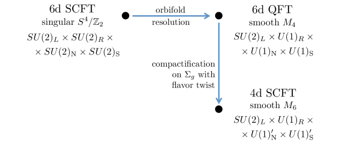
Figure 1: Schematic representation of the construction considered in this work. The starting point is the 6d (1,0) SCFT living on a stack of M5-branes probing the singularity $\mathbb{C}^{2}/\mathbb{Z}_{2}$. We move away from the 6d conformal point by resolving the two orbifolds points of $S^{4}/\mathbb{Z}_{2}$ while preserving 6d (1,0) supersymmetry. Finally, we compactify on the Riemann surface $\Sigma_{g}$ with a suitable flavor twist. For each theory we give the associated internal space and the global symmetry group. The factors $U(1)^{\prime}_{\mathrm{N}}\times U(1)^{\prime}_{\mathrm{S}}$ are defined in (1.1).

The orbifold singularities at the north and south poles can be resolved in a canonical way preserving 6d (1,0) supersymmetry. The orbifold $S^{4}/\mathbb{Z}_{2}$ is replaced by a smooth internal space $M_{4}$. In the resolved phase, the flavor symmetry $SU(2)_{\mathrm{N}}\times SU(2)_{\mathrm{S}}$ is broken to its Cartan subgroup $U(1)_{\mathrm{N}}\times U(1)_{\mathrm{S}}$. The 4d theories of interest in this work are obtained by reducing the 6d theory in its resolved phase by compactification on a smooth genus-$g$ Riemann surface $\Sigma_{g}$ (with $g\neq 1$). The compactification includes a twist for the $U(1)_{\mathrm{N}}\times U(1)_{\mathrm{S}}$ flavor symmetry, while $SU(2)_{L}$ is untwisted. The resulting 4d theories are then labelled by the genus $g$ and three flux quanta $N$, $N_{\mathrm{N}}$, $N_{\mathrm{S}}$, with $N$ the number of M5-branes in the stack, and $N_{\rm N,S}$ the twist parameter for the flavor symmetry $U(1)_{\rm N,S}$. The internal space $M_{4}$ of the resolved 6d theory is non-trivially fibered over the Riemann surface, yielding a 6d space $M_{6}$, with $M_{4}\hookrightarrow M_{6}\rightarrow\Sigma_{g}$. Our construction is summarized schematically in figure 1.

The global symmetries of the 4d QFT are encoded in the geometry and topology of the space $M_{6}$. We notice that the global symmetries of the 4d QFT correspond to gauge symmetries of the 5d supergravity obtained by reduction of M-theory on the internal space $M_{6}$. In this 5d supergravity theory, we have a massless gauge field for each isometry generator of $M_{6}$. Furthermore, additional 5d gauge fields are obtained by expanding the M-theory 3-form $C_{3}$ onto harmonic 2-forms in $M_{6}$.

The space $M_{6}$ has isometry group $U(1)_{R}\times SU(2)_{L}$, which is simply identified with the subgroup of the 6d isometry group $SU(2)_{R}\times SU(2)_{L}$ that is preserved by twisting over the Riemann surface. The space $M_{6}$ also admits three harmonic 2-forms, denoted $\omega_{\mathrm{N}}$, $\omega_{\mathrm{S}}$, $\omega_{\mathrm{C}}$. The 2-forms $\omega_{\rm N,S}$ can be traced back to the resolution of the orbifold singularities of $S^{4}/\mathbb{Z}_{2}$ of the parent 6d theory. The 2-form $\omega_{\mathrm{C}}$, on the other hand, only emerges after reduction to four dimensions, by fibering $M_{4}$ non-trivially over $\Sigma_{g}$. From a field theory point of view, the existence of a third harmonic 2-form in the 4d setup is interpreted as the emergence of an accidental $U(1)_{C}$ global symmetry, which is not visible in six dimensions.

A crucial feature of the 5d supergravity theory obtained from compactification on $M_{6}$ is the following. While all three harmonic 2-forms $\omega_{\mathrm{N}}$, $\omega_{\mathrm{S}}$, $\omega_{\mathrm{C}}$ yield a 5d vector, one linear combination of such vectors gets massive via Stückelberg mechanism, by coupling to a 5d axion. This phenomenon is described in greater detail in Bah:2019rgq . From a field theory perspective, the symmetry group $U(1)_{\mathrm{N}}\times U(1)_{\mathrm{S}}\times U(1)_{\mathrm{C}}$ is spontaneouly broken to a $U(1)^{\prime}_{\mathrm{N}}\times U(1)^{\prime}_{\mathrm{S}}$ subgroup. The connection between Stückelberg mechanism in 5d supergravity, and spontaneous symmetry breaking of global symmetries in the 4d theory, is well-established in the holography literature, see e.g. Gubser:2008px ; Hartnoll:2008vx . To summarize,

$$U(1)_{\mathrm{N}}\times U(1)_{\mathrm{S}}\;\xrightarrow[\;\;\;\;\phantom{l}\text{symmetry}\phantom{l}\;\;\;\;]{\phantom{p}\text{accidental}\phantom{p}}\;U(1)_{\mathrm{N}}\times U(1)_{\mathrm{S}}\times U(1)_{\mathrm{C}}\;\xrightarrow[\text{symm.~{}breaking}]{\text{spontaneous}}\;U(1)^{\prime}_{\mathrm{N}}\times U(1)^{\prime}_{\mathrm{S}}\ ,$$

with the generators $T^{\prime}_{\rm N,S}$ of $U(1)^{\prime}_{\rm N,S}$ given in terms of the generators $T_{\rm N,S,C}$ of $U(1)_{\rm N,S,C}$ as

$$T^{\prime}_{\mathrm{N}}=T_{\mathrm{N}}-\frac{N_{\mathrm{N}}}{N}\,T_{\mathrm{C}}\ ,\qquad T^{\prime}_{\mathrm{S}}=T_{\mathrm{S}}-\frac{N_{\mathrm{S}}}{N}\,T_{\mathrm{C}}\ .$$ (1.1)

The naïve symmetry $U(1)_{\mathrm{N}}\times U(1)_{\mathrm{S}}$ visible in 6d dimensions is replaced by $U(1)^{\prime}_{\mathrm{N}}\times U(1)^{\prime}_{\mathrm{S}}$. Even though the rank is unchanged, this process has deep implications for the ’t Hooft anomalies of the theory, due to the non-trivial mixing of generators in (1.1).

We perform a careful analysis of the ’t Hooft anomalies of the 4d QFT, using the techniques developed in Bah:2019rgq , based on anomaly inflow from the M-theory ambient space. The main idea in Bah:2019rgq is to obtain the inflow anomaly polynomial $I_{6}^{\rm inflow}$ of the 4d QFT by integrating a 12-form characteristic class $\mathcal{I}_{12}$, which encodes the anomalous variation of the M-theory action in the presence of the M5-brane stack. Crucially, $I_{6}^{\rm inflow}$ counterbalances the anomalies of all degrees of freedom living on the stack, which in the IR can be organized into the interacting QFT of interest, plus possible decoupled sectors. We may then write

$$I_{6}^{\rm inflow}=\int_{M_{6}}\mathcal{I}_{12}\ ,\qquad I_{6}^{\rm inflow}+I_{6}^{\rm QFT}+I_{6}^{\rm decoupl}=0\ .$$ (1.2)

While we do not have a complete understanding of decoupled sectors, we can assume that their contribution to the ’t Hooft anomalies is subleading in the large-$N$ limit, which is taken as $N,N_{\rm N,S}\rightarrow\infty$, keeping $N_{\rm N,S}/N$ finite. Under this assumption, the term $I_{6}^{\rm decoupl}$ in (1.2) can be neglected at leading order at large $N$, and we can infer the anomaly polynomial of the interacting QFT from $I_{6}^{\rm inflow}$.

In order to test our large-$N$ result, we investigate the gravity duals of our 4d field theory constructions. As it turns out, we identify the gravity duals to be a well-known class of $AdS_{5}$ solutions in M-theory, first discussed in Gauntlett-Martelli-Sparks-Waldram (GMSW) Gauntlett:2004zh . These solutions are warped products $AdS_{5}\times_{w}M_{6}^{\rm hol}$, where the internal space $M_{6}^{\rm hol}$ is smooth and has exactly the same topology and isometries as $M_{6}$ in the probe M5-brane picture. The existence of smooth dual geometries provides evidence that our construction yields a non-trivial interacting 4d SCFT in the IR, at least at large $N$.

To give more supporting evidence for our claims, we carry out two quantitative checks, by computing the central charge $c$ and the flavor central charge for the global symmetry $SU(2)_{L}$ of the 4d theory. These quantities can be computed holographically at large $N$ from the supergravity effective action. On the field theory side, they can be extracted from the anomaly polynomial, because the superconformal algebra relates them to ’t Hooft anomalies coefficients involving the $SU(2)_{L}$ generators and the superconformal R-symmetry Anselmi:1996dd ; Anselmi:1997rd . The latter is the linear combination of $U(1)_{R}\times U(1)^{\prime}_{\mathrm{N}}\times U(1)^{\prime}_{\mathrm{S}}$ determined by $a$-maximization Intriligator:2003jj . We find a perfect agreement between the supergravity and field theory computations, at leading order in the large-$N$ expansion.

The outcome of $a$-maximization depends crucially on the mixing (1.1) of the naïve symmetry generators $T_{\rm N,S}$ of $U(1)_{\rm N,S}$ with the generator $T_{\mathrm{C}}$ of the emergent $U(1)_{\mathrm{C}}$ symmetry. In particular, in order to match the supergravity results it is essential to take into account emergent symmetries and spontaneous symmetry breaking in the computation of the ’t Hooft anomalies of the 4d theory. The methods of Bah:2019rgq provide a streamlined, geometric way of addressing these phenomena. Indeed, if we integrate the anomaly polynomial of the parent 6d SCFT of $\Sigma_{g}$, we do not reproduce the correct large-$N$ central charge from holography.

The rest of this paper is organized as follows. In section 2 we describe the 6d M-theory setup with a stack of $N$ M5-branes probing a $\mathbb{C}^{2}/\mathbb{Z}_{2}$ singularity. Section 3 is devoted to the reduction of the 6d theory to four dimensions on $\Sigma_{g}$, and to the global symmetries of the 4d QFT. In section 4 we compute the anomalies of the 4d QFT using inflow. In section 5 we identify the gravity duals and we perform the aforementioned quantitative tests involving the central charges of the 4d theories. We conclude with a brief discussion in section 6. The computations in supergravity are collected in appendix A.

2 Six-dimensional setup

The main setup of interest is a stack of $N$ M5-branes probing a $\mathbb{C}^{2}/\mathbb{Z}_{2}$ orbifold singularity in M-theory. First, we discuss some general aspects where the M5-branes are probing a $\mathbb{C}^{2}/\mathbb{Z}_{k}$ orbifold fixed point.

2.1 Aspects of M-theory on $\mathbb{C}^{2}/\mathbb{Z}_{k}$

First we consider the M-theory background with the orbifold $\mathbb{C}^{2}/\mathbb{Z}_{k}$. Let $(x^{0},\cdots,x^{5})$ be the coordinates along an $\mathbb{R}^{6}$ plane, and $(y^{1},\cdots,y^{5})$ be the coordinates along the transverse directions. The latter parametrize a five-dimensional space $\mathbb{C}^{2}\times\mathbb{R}$ with complex coordinates $(z_{1}=y^{1}+iy^{2},z_{2}=y^{3}+iy^{4})$. The orbifold action is

$$(z_{1},z_{2},y^{5})\sim(e^{\frac{2\pi i}{k}}z_{1},e^{-\frac{2\pi i}{k}}z_{2},y^{5}).$$ (2.1)

A local metric for the M-theory background is given as

$$ds^{2}_{11} =ds^{2}(\mathbb{R}^{6})+dr^{2}+r^{2}\,ds^{2}(S^{4}/\mathbb{Z}_{k})$$ (2.2)

$$ds^{2}(S^{4}/\mathbb{Z}_{k}) =\frac{d\mu^{2}}{1-\mu^{2}}+(1-\mu^{2})\left[\frac{1}{k^{2}}\,D\varphi^{2}+\frac{1}{4}\,ds^{2}(S^{2}_{\psi})\right],$$ (2.3)

$$ds^{2}(S^{2}_{\psi}) =d\theta^{2}+\sin^{2}\theta\,d\psi^{2},\qquad D\varphi=d\varphi+\frac{k}{2}\cos\theta\,d\psi.$$ (2.4)

The radius $r$ is constructed from $y^{5}$ and the radii of the two complex planes, in particular we have $y^{5}=r\mu$. The circle coordinates have periodicity $(\Delta\psi=2\pi,\Delta\varphi=2\pi)$. For $k=1$, the metric (2.3) is that of round four-sphere. When $k>1$, the orbifold action admits two $\mathbb{R}^{4}/\mathbb{Z}_{k}$ fixed points at the poles of the sphere at $\mu=\pm 1$. At constant values of $\mu$, the three dimensional sections of the four-sphere are $S^{1}_{\phi}$ bundles over $S^{2}_{\psi}$ with degree $k$. The isometries of $S^{1}_{\varphi}$ and $S^{2}_{\psi}$ lead to a $U(1)_{\varphi}\times SU(2)_{\psi}$ gauge symmetry on the extended seven-dimensional directions of the M-theory background. This is the subgroup of the $SO(5)$ isometry of the sphere preserved by the orbifold action.

The region near an orbifold fixed point of the sphere corresponds to a single center Taub-NUT space, the metric near each pole is

$$ds^{2}\cong\frac{1}{V}\,D\varphi^{2}+V\,\left[dR^{2}+R^{2}\,ds^{2}(S^{2}_{\psi})\right]\ ,\quad V=\frac{k}{2R}\ ,\quad R=\frac{1}{k}\,(1\mp\mu)\ ,\quad\mbox{for}\quad\mu=\pm 1\ .$$ (2.5)

The orbifold singularities can be resolved locally by replacing the single center Taub-NUT space to a Gibbons-Hawking space with $k$ sources of unit charge. Such spaces are $S^{1}_{\varphi}$ bundles over $\mathbb{R}^{3}$ with metric given as

$$ds^{2}=V^{-1}\left(d\varphi+A\right)^{2}+V\left(dX^{2}+dY^{2}+dZ^{2}\right)\ ,\qquad\mbox{with}\quad dV=\star_{\mathbb{R}^{3}}dA\ ,$$ (2.6)

where $V$ is a potential on the 3D base space and $A$ is a connection one-form for the circle bundle. The potential satisfies Laplace’s equation on the $\mathbb{R}^{3}$ base. A general solution of Gibbons-Hawking space is given by inserting $k$ centers at positions $\vec{X}_{I}=(X_{I},Y_{I},Z_{I})$ with charge $n^{I}$. The potential is

$$V=v_{0}+\frac{1}{2}\sum_{I}\frac{n^{I}}{\big{|}\vec{X}-\vec{X}_{I}\big{|}}\ .$$ (2.7)

The parameter $v_{0}$ fixes the asymptotic size of the circle. The coordinate $\varphi$ has period $2\pi$. The space is Asymptotically Locally Flat (ALF) when $v_{0}\neq 0$ with topology of $S^{1}\times\mathbb{R}^{3}$, and asymptotically Locally Euclidean (ALE) when $v_{0}=0$ with topology of $\mathbb{R}^{4}$.

The region near each center is described by a $\mathbb{R}^{4}/\mathbb{Z}_{n^{I}}$ orbifold fixed point where $S^{1}_{\varphi}$ shrinks. A two-cycle can be obtained by taking $S^{1}_{\varphi}$ with a segment on $\mathbb{R}^{3}$ that connects two singularities. There are $k-1$ independent two-cycles with harmonic representatives, $\omega^{i}$ $(i\in\{1,\cdots,k-1\})$. When all $n^{I}=1$, the space is smooth with $k-1$ two-cycles. This corresponds to a resolution of the orbifold singularity. The $S^{1}_{\psi}$ circle of $S^{2}_{\psi}$ in 2.5, is identified with the rotation on the $(X,Y)$ plane. Resolving the singularity breaks the $SU(2)_{\psi}$ isometry of $S^{2}_{\psi}$ to a $U(1)_{\psi}$ corresponding to the rotations of $S^{1}_{\psi}$.

M-theory, in the supergravity limit, can be studied on the space (2.2) where we replace the two orbifold singularities with their smooth resolutions. This local deformation is always possible since the asymptotic space of Gibbons-Hawking is fixed by the total charge. M-theory has a 2-form gauge symmetry with a 3-form potential, $C_{3}$. There are massless fluctuations of the $C_{3}$ potential on the extended seven-dimensional space coming from the resolutions of the singularities. In reducing M-theory on the compact space, we can add terms to $C_{3}$ as

$$C_{3}=a_{i}^{\mathrm{N}}\wedge\omega^{i}_{\mathrm{N}}+a_{i}^{\mathrm{S}}\wedge\omega^{i}_{\mathrm{S}}+\cdots$$ (2.8)

where $(\omega_{\mathrm{N}}^{i},\omega_{\mathrm{S}}^{i})$ are the resolution harmonic two-forms for the north and south singularities, respectively. The one-forms $(a^{\mathrm{N}}_{i},a^{\mathrm{S}}_{i})$ are massless gauge field on the seven-dimensional space. Each orbifold fixed point leads to a $U(1)^{k-1}$ gauge symmetry in M-theory which enhances to an $SU(k)$ gauge symmetry in the singular limit Sen:1997kz . To summarize, the M-theory background admits an $SU(2)_{\psi}\times SU(k)_{\mathrm{N}}\times SU(k)_{\mathrm{S}}\times U(1)_{\varphi}$ bosonic gauge symmetry.

We are interested in the field theory that describe the low energy dynamics of a stack of $N$ M5-branes probing the M-theory singularity at $r=0$ in (2.2). The gauge symmetry of the M-theory background induces a global symmetry on the worldvolume directions of the M5-branes. The $SU(2)_{\psi}$ symmetry from $S^{2}_{\psi}$ corresponds to an $SU(2)_{\mathcal{R}}$ R-symmetry, whiles the rest $SU(k)_{\mathrm{N}}\times SU(k)_{\mathrm{S}}\times U(1)_{\varphi}$ imprints as a flavor symmetry. In particular, the 7d gauge fields $(a^{\mathrm{N}}_{i},a^{\mathrm{S}}_{i})$ yield 6d background connections $(A^{\mathrm{N}}_{6d\,i},A^{\mathrm{S}}_{6d\,i})$. This configuration preserves eight supercharges leading to a six-dimensional superconformal field theory with a $(1,0)$ supersymmetry Brunner:1997gk ; Blum:1997fw ; Blum:1997mm ; Intriligator:1997dh ; Brunner:1997gf ; Hanany:1997gh .

2.2 The case $k=2$

The resolution space of $S^{4}/\mathbb{Z}_{2}$ has an enhanced symmetry. The $U(1)_{\varphi}$ isometry of $S^{1}_{\varphi}$ in $S^{4}/\mathbb{Z}_{2}$ enhances to an $SU(2)_{\varphi}$ isometry group as can be seen by rewriting the metric as

$$ds^{2}(S^{4}/\mathbb{Z}_{2})=\frac{d\mu^{2}}{1-\mu^{2}}+\frac{1}{4}\,(1-\mu^{2})\,\left[D\psi^{2}+d\theta^{2}+\sin^{2}\theta\,d\varphi^{2}\right],\quad D\psi=d\psi+\cos\theta\,d\psi.$$ (2.9)

The resolution of the orbifold singularities at $\mu=\pm 1$ preserve the isometries of $S^{2}_{\varphi}$ composed of $(\theta,\psi)$ in the metric of $S^{4}/\mathbb{Z}_{2}$ above. This follows from the fact that the resolution space of $\mathbb{R}^{4}/\mathbb{Z}_{2}$ is the Eguchi-Hanson space Eguchi:1978xp . To see this more explicitly, write the potentials for the two center Gibbons-Hawking space with unit charge as

$$V =\frac{1}{2R_{+}}+\frac{1}{2R_{-}},\qquad A=\frac{1}{2}\left(\frac{Z_{+}}{R_{+}}+\frac{Z_{-}}{R_{-}}\right)d\tan^{-1}\left(Y/X\right)\ ,$$ (2.10)

$$R_{\pm}^{2} =X^{2}+Y^{2}+Z_{\pm}^{2}\ ,\qquad Z_{\pm}=Z\pm Z_{0}\ .$$ (2.11)

The centers are sitting at $(0,0,\pm Z_{0})$. The metric of the resolved space can be written as

$$ds^{2}=\frac{R^{4}}{R^{4}-a^{4}}\,dR^{2}+\frac{R^{2}}{4}\,\left[d\theta^{2}+\sin^{2}\theta\,d\varphi^{2}+\frac{R^{4}-a^{4}}{R^{4}}\left(d\psi+\cos\theta\,d\varphi\right)^{2}\right]\ ,$$ (2.12)

where we have made the coordinate transformation Prasad:1979kg

$$Z=\frac{R^{2}}{4}\,\cos\theta\ ,\quad X=\frac{\sqrt{R^{4}-a^{4}}}{4}\,\sin\theta\,\cos\psi\ ,\quad Y=\frac{\sqrt{R^{4}-a^{4}}}{4}\,\sin\theta\,\sin\psi\ .$$ (2.13)

The space smoothly caps off at $R=a$ where the $S^{1}_{\psi}$ circle shrinks. The two-sphere, $S^{2}_{\varphi}$, composed of $(\theta,\varphi)$ in the resolved space has a finite size of $a/2$ at $R=a$. The two-sphere in this region also corresponds to the two-cycle of the resolution of the $\mathbb{R}^{4}/\mathbb{Z}_{2}$.

The singularities of $S^{4}/\mathbb{Z}_{2}$ are resolved by excising the singular region and gluing in the Eguchi-Hanson space describe in (2.12). The $S^{2}_{\varphi}$ of (2.12) is identified with the $S^{2}_{\varphi}$ of $S^{4}/\mathbb{Z}_{2}$ in (2.9). In this sense, the resolution of the singularities on the sphere preserves its isometries.

The smooth geometry obtained from the resolution of $S^{4}/\mathbb{Z}_{2}$ is denoted as $M_{4}$. It has the topology of $S^{2}\times S^{2}$ and corresponds to the Hirzebruch surface $\mathbb{F}_{2}$. It is useful to write a local metric for the space $M_{4}$,

$$ds^{2}(M_{4})=h_{1}(\mu)\,ds^{2}(S^{2}_{\varphi})+h_{2}(\mu)\,d\mu^{2}+h_{3}(\mu)\,D\psi^{2}\ ,\qquad D\psi =d\psi+\cos\theta\,d\varphi\ .$$ (2.14)

The coordinate $\mu$ takes value in the interval $[\mu_{\mathrm{S}},\mu_{\mathrm{N}}]$. The boundary conditions of the $h$’s are fixed by regularity of the metric at the bounds, and in particular, $h_{3}$ must vanish on them. The two-sphere $S^{2}_{\varphi}$ is not shrinking at the north and south poles of $M_{4}$ where the $S^{1}_{\psi}$ is shrinking. The two-spheres at the tip of the $\mu$-interval correspond to two-cycles denoted as $(\mathcal{S}^{2}_{\mathrm{S}},\mathcal{S}^{2}_{\mathrm{N}})$ respectively. The volume of these cycles are then $(h_{1}(\mu_{\mathrm{S}}),h_{1}(\mu_{\mathrm{N}}))$ respectively.

The sizes of the two-cycles $(\mathcal{S}^{2}_{\mathrm{S}},\mathcal{S}^{2}_{\mathrm{N}})$ are moduli parameters of $M_{4}$. In the singular limit where they vanish, $M_{4}\to S^{4}/\mathbb{Z}_{2}$. The four-sphere admits a left $SU(2)$ and a right $SU(2)$ action; these are preserved by the $\mathbb{Z}_{2}$ orbifold action, and are related to the isometries of $SU(2)_{\psi}\times SU(2)_{\varphi}$ rotations. The $U(1)_{\psi}\times SU(2)_{\varphi}$ are manifest as isometries of $S^{1}_{\psi}\times S^{2}_{\varphi}$ of the metric (2.9). The total gauge symmetry in seven dimensions is $SU(2)_{\psi}\times SU(2)_{\varphi}\times SU(2)_{\mathrm{N}}\times SU(2)_{\mathrm{S}}$.

Anomalies of the 6d setup

Anomaly inflow for flat M5-branes probing orbifold singularities was studied in Ohmori:2014kda . See also Bah:2019rgq for a review of the computation. The inflow computation yields an 8-form $I_{8}^{\rm inflow}$ which captures the variation of the M-theory action in the presence of the M5-brane stack. The inflow anomaly polynomial counterbalances the anomalies of the worldvolume degrees of freedom, which at low energies consists of an interacting SCFT and of modes that decouple in the IR,

$$I_{8}^{\rm inflow}+I_{8}^{\rm SCFT}+I_{8}^{\rm decoupl}=0\ .$$ (2.15)

The inflow anomaly polynomial reads

$$-I_{8}^{\rm inflow} =\frac{N^{3}}{6}\,\big{[}c_{2}^{\varphi}-c_{2}^{\psi}\big{]}^{2}+\frac{N}{12}\,\big{[}4\,c_{2}^{\varphi}-3\,c_{2}^{\psi}\big{]}\,c_{2}^{\psi}+\frac{N}{24}\,\big{[}2\,c_{2}^{\varphi}-\,c_{2}^{\psi}\big{]}\,p_{1}(TW_{6})$$

$$-\frac{1}{32\,N}\,\bigg{[}\frac{{\rm tr}\,(F_{6d}^{\rm N})^{2}}{(2\pi)^{2}}-\frac{{\rm tr}\,(F_{6d}^{\rm S})^{2}}{(2\pi)^{2}}\bigg{]}^{2}+\frac{N}{4}\,\big{[}c_{2}^{\varphi}-c_{2}^{\psi}\big{]}\,\bigg{[}\frac{{\rm tr}\,(F_{6d}^{\rm N})^{2}}{(2\pi)^{2}}+\frac{{\rm tr}\,(F_{6d}^{\rm S})^{2}}{(2\pi)^{2}}\bigg{]}$$

$$+\frac{N}{192}\big{[}p_{1}(TW_{6})^{2}-4\,p_{2}(TW_{6})\big{]}\ .$$ (2.16)

We have introduced the compact notation

$$c_{2}^{\varphi}\equiv c_{2}(SU(2)_{\varphi})\ ,\qquad c_{2}^{\psi}\equiv c_{2}(SU(2)_{\psi})\ .$$ (2.17)

The anomaly of the decoupling modes is given by

$$I_{8}^{\rm decoupl} =I^{\rm tensor}_{8}+\frac{1}{2}\,I_{8}^{\rm vec,N}+\frac{1}{2}\,I_{8}^{\rm vec,S}\ .$$ (2.18)

The 8-form $I^{\rm tensor}_{8}$ is the anomaly polynomial of a 6d (1,0) tensor multiplet,

$$I_{8}^{\rm tensor}=\frac{1}{24}\,(c_{2}^{\psi})^{2}+\frac{1}{48}\,c_{2}^{\psi}\,p_{1}(TW_{6})+\frac{23}{5760}\,p_{1}(TW_{6})^{2}-\frac{29}{1440}\,p_{2}(TW_{6})\ .$$ (2.19)

The 8-form $I_{8}^{\rm vec,N}$ is the anomaly polynomial of a 6d (1,0) vector multiplet of $SU(2)_{\mathrm{N}}$,

$$I_{8}^{\rm vec,N} =-\frac{1}{8}\,(c_{2}^{\psi})^{2}-\frac{1}{16}\,c_{2}^{\psi}\,p_{1}(TW_{6})-\frac{1}{1920}\big{[}7\,p_{1}(TW_{6})^{2}-4\,p_{2}(TW_{6})\big{]}$$

$$-\frac{1}{2}\,c_{2}^{\psi}\,\frac{{\rm tr}\,(F_{6d}^{N})^{2}}{(2\pi)^{2}}-\frac{1}{24}\,p_{1}(TW_{6})\,\frac{{\rm tr}\,(F_{6d}^{N})^{2}}{(2\pi)^{2}}-\frac{1}{12}\,\bigg{[}\frac{{\rm tr}\,(F_{6d}^{N})^{2}}{(2\pi)^{2}}\bigg{]}^{2}\ .$$ (2.20)

The quantity $I_{8}^{\rm vec,S}$ is completely analogous.

3 Four-dimensional setup

In this section we describe aspects of the geometric setup when a stack of $N$ M5-branes wrapping a genus, $g$, Riemann Surface $\Sigma_{g,n}$ with $n$ punctures, probe a $\mathbb{C}^{2}/\mathbb{Z}_{2}$ singularity in M-theory. We will discuss various aspects of the geometric setup in M-theory and the symmetries they induce for the field theory that describe the low-energy dynamics of the branes. We will then use the geometric set-up and compute the anomaly polynomial of the field theory by using anomaly inflow techniques developed in Bah:2019rgq .

3.1 Geometric setup for 4d systems

We consider an eleven-dimensional background given as

$$M_{11}=W_{4}\times\Sigma_{g,n}\times\mathbb{C}^{2}/\mathbb{Z}_{2}\times\mathbb{R}.$$ (3.1)

The M-theory background preserves supersymmetry when the space $\Sigma_{g,n}\times\mathbb{C}^{2}/\mathbb{Z}_{2}$ satisfies the Calabi-Yau threefold condition, i.e. the first Chern class of the space must vanish. The worldvolume of the branes decompose as $W_{6}=W_{4}\times\Sigma_{g,n}$ where $W_{4}$ is the external spacetime. The low-energy dynamics of the branes is captured by a field theory that live on $W_{4}$. In the region near the branes, the spacetime decomposes as

$$M_{11}=\mathbb{R}^{+}\times M_{10},\quad\mbox{where}\quad M_{6}\hookrightarrow M_{10}\rightarrow W_{4},\quad M_{4}\hookrightarrow M_{6}\rightarrow\Sigma_{g,n}.$$ (3.2)

The line $\mathbb{R}^{+}$ is the overall radius of the transverse directions of the worldvolume spacetime $W_{4}$. The space $M_{10}$ describes the tubular neighborhood of the branes, it also corresponds to an internal boundary of the M-theory spacetime near the branes. Finally, $M_{4}$ is the resolution space of $S^{4}/\mathbb{Z}_{2}$ describe in section 2.2.

The Calabi-Yau condition on the M-theory background is satisfied by twisting the R-symmetry circle $S^{1}_{\psi}$ over the Riemann surface. This twist breaks the six-dimensional $SU(2)_{\mathcal{R}}$ R-symmetry to a $U(1)_{\mathcal{R}}$ symmetry for the worldvolume theory on $W_{4}$. At the level of the geometry, this is achieved by shifting the connection of $S^{1}_{\psi}$ as

$$D\psi\;\to\;\widehat{D}\psi=d\psi+\cos\theta\,d\varphi-2\pi\,\chi\,A_{\Sigma}\ ,\quad\mbox{with}\quad\int_{\Sigma_{g,n}}dA_{\Sigma}=1\ ,\quad\chi=-2(g-1)-n\ .$$ (3.3)

The Euler characteristic of the Riemann surface is denoted by $\chi$. The twisting, $A_{\Sigma}$, is a nontrivial component of the six-dimensional gauging of the R-symmetry of the 6d theory.

In addition to twisting the R-symmetry, a large family of four-dimensional SCFTs can be engineered by turn on background fields along the Riemann surface for the Cartan elements of the $SU(2)_{\mathrm{N}}\times SU(2)_{\mathrm{S}}\times SU(2)_{\varphi}$ flavor symmetry. Such background fields break the flavor symmetry of the six-dimensional theory to $U(1)_{\mathrm{N}}\times U(1)_{\mathrm{S}}\times U(1)_{\varphi}$ for the four-dimensional theory. At the level of the M-theory background, this is achieved by turning on the following flux parameters

$$d\varphi\to\widehat{D}\varphi =d\varphi+2\pi\,z\,A_{\Sigma}$$ (3.4)

$$C_{3}\to\widehat{C}_{3} =C_{3}+2\pi\,(N_{\mathrm{N}}\,A_{\Sigma}\wedge\omega_{\mathrm{N}}+N_{\mathrm{S}}\,A_{\Sigma}\wedge\omega_{\mathrm{S}})\ .$$ (3.5)

The connection forms $(N_{\mathrm{N}}\,A_{\Sigma},N_{\mathrm{S}}\,A_{\Sigma})$ are background fields for the $U(1)$ gauge fields discussed in (2.8) in the case of $k=2$. The two-forms $(\omega_{\mathrm{N}},\omega_{\mathrm{S}})$ are the closed representatives that measure the volumes of the resolution two-cycles $(\mathcal{S}_{\mathrm{N}}^{2},\mathcal{S}_{\mathrm{S}}^{2})$ in $M_{4}$. For every choice of a Riemann surface, $\Sigma_{g,n}$, there is a family of four-dimensional systems labeled by the three flux parameters $(z,N_{\mathrm{N}},N_{\mathrm{S}})$ and the number of branes, $N$.

In this paper, we restrict to four-dimensional theories that preserve the $SU(2)_{\varphi}$ symmetry, this corresponds to fixing $z=0$. We will also restricted to cases with no punctures, i.e. $n=0$, and non-vanishing curvature, $g\neq 0$. For this family, a local metric for $M_{6}$ can be written as

$$ds^{2}(M_{6})=h_{0}(\mu)ds^{2}(\Sigma_{g})+h_{1}(\mu)ds^{2}(S^{2}_{\varphi})+h_{2}(\mu)d\mu^{2}+h_{3}(\mu)\widehat{D}\psi^{2}.$$ (3.6)

The interval $\mu$ takes value in $[\mu_{\mathrm{S}},\mu_{\mathrm{N}}]$ where the endpoints are fixed by the loci where $h_{3}$ vanish. The functions $(h_{0},h_{1})$ parametrize the radii of $\Sigma_{g}$ and $S^{2}_{\varphi}$ in $M_{6}$, they are non-vanishing on the interval of $\mu$.

At a fixed point on the surface $\Sigma_{g}$, there is a fiber that is a copy of $M_{4}$ composed of $S^{2}_{\varphi}$, the circle $S^{1}_{\psi}$ and the interval $\mu$. Similarly, we can consider a fixed point on the sphere $S^{2}_{\psi}$, there are four-dimensional fibers which are copies of a space $M_{4}^{\Sigma}$ which are composed of the Riemann surface $\Sigma_{g}$, the circle $S^{1}_{\psi}$ and the interval $\mu$. These fibers do not shrink in $M_{6}$.

3.2 Flux quantization and four-cycles of $M_{6}$

One of the main object of interest is the boundary condition for the four-flux $G_{4}$ when the branes wrap the Riemann surface. Following Freed:1998tg ; Harvey:1998bx , we can write the boundary term for $G_{4}$ by using a bump function $\rho(r)$ as

$$G_{4}=2\pi\rho(r)\,\overline{G}_{4}+\dots,\qquad\mbox{with}\qquad\int_{M_{4}}\overline{G}_{4}=N\ .$$ (3.7)

The flux $\overline{G}_{4}$ supports the non-trivial geometry $M_{6}$.

The space $M_{4}$ is the fiber over the Riemann Surface, $\Sigma_{g}$. Since it is non-shrinking, we can thread $N$ units of flux on it at a fixed point of the Riemann surface. Similarly, at a fixed point of the sphere, $S^{2}_{\varphi}$, we can thread flux on the fiber $M_{4}^{\Sigma}$ given as

$$\int_{M_{4}}\overline{G}_{4}=N_{\Sigma}.$$ (3.8)

The space $M_{6}$ also admits four-cycles localized at the north and south poles of the $\mu$ interval where $S^{1}_{\psi}$ shrinks. These correspond to the product of the resolution cycles of the original orbifold singularities of the $S^{4}/\mathcal{Z}_{2}$ with the Riemann surface, $\Sigma_{g}$. They are denoted as

$$\mathcal{C}_{\mathrm{N}}^{4} =\mathcal{S}^{2}_{\mathrm{N}}\times\Sigma_{g} \mbox{localized at}\qquad\mu=\mu_{\mathrm{N}}\ ,$$ (3.9)

$$\mathcal{C}_{\mathrm{S}}^{4} =\mathcal{S}^{2}_{\mathrm{S}}\times\Sigma_{g} \mbox{localized at}\qquad\mu=\mu_{\mathrm{S}}\ .$$ (3.10)

We can thread flux on these cycles given as

$$\int_{\mathcal{C}_{\mathrm{N}}^{4}}\overline{G}_{4}=N_{\mathrm{N}}\in\mathbb{Z},\qquad\int_{\mathcal{C}_{\mathrm{S}}^{4}}\overline{G}_{4}=N_{\mathrm{S}}\in\mathbb{Z}.$$ (3.11)

It seems then that there exist four flux quanta $(N,N_{\Sigma},N_{\mathrm{N}},N_{\mathrm{S}})$ that label the class of $\overline{G}_{4}$ in $M_{6}$. These flux parameters are not all independent. This reflects the fact that the space $M_{6}$ actually admits only three four-cycles denoted as $(\mathcal{C}_{\mathrm{N}}^{4},\mathcal{C}_{\mathrm{S}}^{4},\mathcal{C}_{\mathrm{C}}^{4})$. The last one $\mathcal{C}_{\mathrm{C}}^{4}$ is not localized on $M_{6}$. It consists of $S^{2}_{\varphi}\times S^{2}_{\mu\psi}$ at a generic point on $\Sigma_{g}$.

To see that there are only three independent flux parameters, we consider the most general local expression for $\overline{G}_{4}$ that is closed and consistent with the symmetries of $M_{6}$

$$\overline{G}_{4}=\bigg{[}d\gamma_{\varphi}\wedge V_{2}^{\varphi}+d\gamma_{\Sigma}\wedge V_{2}^{\Sigma}\bigg{]}\wedge\frac{\widehat{D}\psi}{2\pi}-(\chi\,\gamma_{\varphi}+2\,\gamma_{\Sigma})\,V_{2}^{\varphi}\wedge V_{2}^{\Sigma}\ ,$$ (3.12)

where $\gamma_{\varphi}$, $\gamma_{\Sigma}$ are functions of $\mu$ only and $V^{\varphi}_{2}$, $V^{\Sigma}_{2}$ are proportional to the volume forms of $S^{2}_{\varphi}$ and the Riemann surface, respectively, normalized according to

$$\int_{S^{2}_{\varphi}}V_{2}^{\varphi}=1\ ,\qquad\int_{\Sigma_{g}}V^{\Sigma}_{2}=1\ .$$ (3.13)

The flux parameters are given as

$$\gamma_{\varphi}^{\mathrm{N}}-\gamma_{\varphi}^{\mathrm{S}}=N\ ,\quad\gamma_{\Sigma}^{\mathrm{N}}-\gamma_{\Sigma}^{\mathrm{S}}=N_{\Sigma}\ ,\quad\chi\,\gamma_{\varphi}^{\mathrm{N}}+2\,\gamma_{\Sigma}^{\mathrm{N}}=-N_{\mathrm{N}}\ ,\quad\chi\,\gamma_{\varphi}^{\mathrm{S}}+2\,\gamma_{\Sigma}^{\mathrm{S}}=-N_{\mathrm{S}}\ ,$$ (3.14)

where the $\gamma$ parameters are defined as $\gamma_{\bullet}^{\rm N,S}\equiv\gamma_{\bullet}(\mu_{\rm N,S})$. The $\gamma$ relations imply

$$2N_{\Sigma}+\chi N=-(N_{\mathrm{N}}-N_{\mathrm{S}})\ .$$ (3.16)

The class $G_{4}$ is labeled by three flux parameters that we denote as $(N,N_{\mathrm{N}},N_{\mathrm{S}})$. The flux parameter $N$ can be associated with the four-cycle $\mathcal{C}_{\mathrm{C}}^{4}$.

The flux parameters can be equivalently regarded as the coefficients of the expansion of $\overline{G}_{4}$ onto coholomogy classes of $M_{6}$,

$$\overline{G}_{4}=N\,\mathcal{V}_{4}^{\mathrm{C}}+N_{\mathrm{N}}\,\mathcal{V}_{4}^{\mathrm{N}}+N_{\mathrm{S}}\,\mathcal{V}_{4}^{\mathrm{S}}+\text{(exact terms)}\ .$$ (3.17)

The 4-forms $\mathcal{V}_{4}^{\alpha}$, $\alpha={\rm N,S,C}$ are closed but not exact, and define a basis of cohomology classes in $M_{6}$. We can parametrize them uniformly by writing

$$\mathcal{V}_{4}^{\alpha}=d\bigg{[}U_{\varphi}^{\alpha}\,V_{2}^{\varphi}\wedge\frac{\widehat{D}\psi}{2\pi}+U_{\Sigma}^{\alpha}\,V_{2}^{\Sigma}\wedge\frac{\widehat{D}\psi}{2\pi}\bigg{]}+C^{\alpha}\,V_{2}^{\varphi}\wedge V_{2}^{\Sigma}\ .$$ (3.18)

In the above expression, $U_{\varphi}^{\alpha}$, $U_{\Sigma}^{\alpha}$ are functions of $\mu$, while $C^{\alpha}$ is constant. The parametrization (3.18) is subject to a 2-parameter redundancy, related to shifts of $U_{\varphi}^{\alpha}$, $U_{\Sigma}^{\alpha}$ by constants. A way to fix this redundancy is to demand

$$(U_{\varphi}^{\alpha})^{\mathrm{N}}+(U_{\varphi}^{\alpha})^{\mathrm{S}}=0\ ,\qquad(U_{\Sigma}^{\alpha})^{\mathrm{N}}+(U_{\Sigma}^{\alpha})^{\mathrm{S}}=0\ .$$ (3.19)

We want the 4-forms $\mathcal{V}_{4}^{\alpha}$ to be dual to the 4-cycles $\mathcal{C}^{4}_{\alpha}$ defined above,

$$\int_{\mathcal{C}^{4}_{\alpha}}\mathcal{V}_{4}^{\beta}=\delta^{\beta}_{\alpha}\ .$$ (3.20)

This condition determines the constants $C^{\alpha}$ and the quantities $(U_{\varphi}^{\alpha})^{\mathrm{N}}$, $(U_{\Sigma}^{\alpha})^{\mathrm{N}}$, according to the following table,

$$\begin{array}[]{l || c | c | ccc}&\phantom{l}(U_{\varphi}^{\alpha})^{\mathrm{N}}\phantom{l}&\phantom{l}(U_{\Sigma}^{\alpha})^{\mathrm{N}}\phantom{l}&\phantom{l}C^{\alpha}\phantom{l}\\[2.84526pt] \hline\cr\alpha=\mathrm{C}\phantom{l}&\frac{1}{2}&-\frac{\chi}{4}&0\\[2.84526pt] \alpha=\mathrm{N}\phantom{l}&0&-\frac{1}{4}&\frac{1}{2}\\[2.84526pt] \alpha=\mathrm{S}\phantom{l}&0&\frac{1}{4}&\frac{1}{2}\end{array}$$ (3.21)

Another way to interpret the fluxes $(N_{\mathrm{N}},N_{\mathrm{S}})$ is to consider the fate of the fluctuations of the $C_{3}$ potential from the $SU(2)_{\mathrm{N}}\times SU(2)_{\mathrm{S}}$ symmetry before the compactification on the Riemann surface. The curvatures associated to $SU(2)_{\mathrm{N}}\times SU(2)_{\mathrm{S}}$ are $(F_{6d}^{\mathrm{N}},F_{6d}^{\mathrm{S}})$. We use the notation $(n_{6d}^{\mathrm{N}},n_{6d}^{\mathrm{S}})$ for the corresponding Chern roots. Since these forms have legs on the worldvolume directions of the M5-branes, $W_{6}$, when we compactify on the Riemann surface, they decompose as Bah:2017gph

$$n^{\mathrm{N}}_{6d}=N_{\mathrm{N}}\,V_{2}^{\Sigma}+N\,\frac{F^{\mathrm{N}}}{2\pi},\qquad n^{\mathrm{S}}_{6d}=N_{\mathrm{S}}\,V_{2}^{\Sigma}+N\,\frac{F^{\mathrm{S}}}{2\pi}\ .$$ (3.22)

The quantities $(F^{\mathrm{N}},F^{\mathrm{S}})$ are 4d external connections. We have introduced a factor $N$ in such a way that both terms on the RHSs of (3.22) scale linearly with the flux parameters $N$, $N^{\mathrm{N}}$, $N^{\mathrm{S}}$. In the reduction, this decomposition implies the flux terms in $\overline{G}_{4}$ as

$$\overline{G}_{4}=N_{\mathrm{N}}\,V_{2}^{\Sigma}\wedge\omega_{\mathrm{N}}+N_{\mathrm{S}}\,V_{2}^{\Sigma}\wedge\omega_{\mathrm{S}}+\dots$$ (3.23)

In field theory, the flux correspond to twisting the Cartan elements of the six-dimensional $SU(2)_{\mathrm{N}}\times SU(2)_{\mathrm{S}}$ symmetry over the Riemann surface.

There are three harmonic two-forms associated to the four-cycles by Poincaré duality, we denote them as $(\omega_{\mathrm{N}},\omega_{\mathrm{S}},\omega_{\mathrm{C}})$. Indeed, the first two are just the resolution two cycles of $M_{4}$ which are preserved in $M_{6}$. The flux quantization conditions can be equivalently written as

$$\int_{M_{6}}\overline{G}_{4}\wedge\omega_{\mathrm{N}}=N_{\mathrm{N}},\qquad\int_{M_{6}}\overline{G}_{4}\wedge\omega_{\mathrm{S}}=N_{\mathrm{S}},\qquad\int_{M_{6}}\overline{G}_{4}\wedge\omega_{\mathrm{C}}=N.$$ (3.24)

These formulas will be useful in the computation of the anomalies for the four-dimensional theories of interest.

In the reduction of M-theory on $M_{6}$, there are a class of fluctuations we can add for the $C_{3}$ potential. For each of the harmonic two-forms, we can add a gauge field in the external spacetime given as $(a^{\mathrm{N}},a^{\mathrm{S}},a^{\mathrm{C}})$ with field strength $(f^{\mathrm{N}},f^{\mathrm{S}},f^{\mathrm{C}})$. We are using lowercase letters to emphasize that these are gauge fields in 7d supergravity. Naively, each one of these fields should lead to a $U(1)$ gauge symmetry on the external spacetime which then induces a $U(1)$ flavor symmetry on the worldvolume theory on the branes. However, the $C_{3}$ potential can also have a three-form fluctuation, $c_{3}$, on the external spacetime with field strength, $g_{4}=dc_{3}$. These terms can be collected as

$$C_{3}=a^{\mathrm{N}}\wedge\omega_{\mathrm{N}}+a^{\mathrm{S}}\wedge\omega_{\mathrm{S}}+a^{\mathrm{C}}\wedge\omega_{\mathrm{C}}+c_{3}+\dots$$ (3.25)

When we reduce the effective action of M-theory, the effective action of the seven-dimensional theory will have terms

$$S=\int b_{1}g_{4}\wedge\star g_{4}+b_{2}N_{\alpha}a^{\alpha}\wedge g_{4}+\dots$$ (3.26)

where the $b$’s are numbers. We observe that $g_{4}$ couples to a linear combination of the gauge field. This coupling implies that $g_{4}$ can be dualized to a Stückelberg field which is eaten by the gauge field $N_{\alpha}a^{\alpha}$. Here and in what follows, the index $\alpha$ enumerates harmonic 2-forms and takes the values $\alpha=\mathrm{N},\mathrm{S},\mathrm{C}$. We refer the reader to Bah:2019rgq for a more detailed discussion of this Stückelberg mechanism.

Symmetries of the system

The low-energy quantum field preserves a $U(1)_{\mathcal{R}}$ R-symmetry and the $SU(2)_{\varphi}$ flavor symmetries corresponding to the isometries of $S^{1}_{\psi}$ and $S^{2}_{\varphi}$. Naively there is an $U(1)_{\mathrm{N}}\times U(1)_{\mathrm{S}}\times U(1)_{\mathrm{C}}$ corresponding to the fluctuations of $C_{3}$ along the harmonic two-forms $(\omega_{\mathrm{N}},\omega_{\mathrm{S}},\omega_{\mathrm{C}})$. One linear combination is broken and only a $U(1)^{2}$ is preserved, which we denote as $U(1)_{\mathrm{N}}\times U(1)_{\mathrm{S}}$. In the special cases when $g=0$, the Riemann surface is a two-sphere, in the low-energy limit it can admit an $SU(2)$ isometry group. The flavor symmetry will further enhance by an $SU(2)$ flavor symmetry.

Now we are in a position to construct the gauge invariant and globally defined boundary condition for the $G_{4}$ flux in presences of curved branes. We have the action of the symmetries in $\overline{G}_{4}$ by adding suitable connection forms and curvature terms to make it closed:

$$\overline{G}_{4}\,\to\,E_{4} =\big{(}d\gamma_{\varphi}\wedge e_{2}^{\varphi}+d\gamma_{\Sigma}\wedge e_{2}^{\Sigma}\big{)}\wedge\,\frac{\widetilde{D}\psi}{2\pi}+\big{(}\gamma_{\varphi}\,e_{2}^{\varphi}+\gamma_{\Sigma}\,e_{2}^{\Sigma}\big{)}\wedge\bigg{(}-2\,e_{2}^{\varphi}-\chi\,e_{2}^{\Sigma}+2\,\frac{F^{\psi}}{2\pi}\bigg{)}$$

$$+N\,\frac{F^{\mathrm{N}}}{2\pi}\wedge\widetilde{\omega}_{\mathrm{N}}+N\,\frac{F^{\mathrm{S}}}{2\pi}\wedge\widetilde{\omega}_{\mathrm{S}}+N\,\frac{F^{\mathrm{C}}}{2\pi}\wedge\widetilde{\omega}_{\mathrm{C}}\ ,\qquad\mbox{with}\quad F^{\alpha}N_{\alpha}=0\ .$$ (3.27)

The last condition imposes the fact that one of gauge fields in the fluctuations of the $C_{3}$ potential is massive. In the expression for $E_{4}$ we have gauged the isometry group as

$$\frac{\widetilde{D}\psi}{2\pi}=\frac{d\psi}{2\pi}-2\,\mathcal{A}^{\varphi}-\chi\,\mathcal{A}^{\Sigma}+2\,\frac{A^{\psi}}{2\pi}\ ,\qquad dA^{\psi}=F^{\psi},\qquad d\mathcal{A}^{\varphi}=e_{2}^{\varphi},\qquad d\mathcal{A}^{\Sigma}=e^{\Sigma}_{2}\ .$$ (3.28)

The quantity $A_{\psi}$ is the 4d connection for $U(1)_{\psi}$. The two-forms, $e^{\varphi}_{2}$ and $e_{2}^{\Sigma}$ are the closed and gauge invariant volume forms of $S^{2}_{\psi}$ and $\Sigma_{g}$ respectively. The expression for $e_{2}^{\varphi}$ is

$$e_{2}^{\varphi}=\frac{1}{8\pi}\,\epsilon_{abc}\,(Dy^{a}\wedge Dy^{b}\,y^{c}-F^{ab}\,y^{c})\ ,\qquad Dy^{a}=dy^{a}-A^{ab}\,y_{b}\ .$$ (3.29)

The indices $a,b,c=1,2,3$ are vector indices of $SO(3)_{\varphi}$, raised and lowered with $\delta_{ab}$. The three quantities $y^{a}$ are constrained coordinates on $S^{2}_{\varphi}$, with $y^{a}\,y_{a}=1$. The 1-forms $A^{ab}$ are the components of the external $SO(3)_{\varphi}$ connection, and $F^{ab}$ are the components of the field strength. When $g>1$, $e_{2}^{\Sigma}$ is simply the volume form on the Riemann surface, $e_{2}^{\Sigma}=V_{2}^{\Sigma}$. When $g=0$ and the surface is a sphere, $e_{2}^{\Sigma}$ is given similarly as (3.29). We need the integrals

$$\int_{\Sigma_{g}}e_{2}^{\Sigma}=1\ ,\qquad\int_{S^{2}}e_{2}^{2s+2}=0\ ,\quad\int_{S^{2}}e_{2}^{2s+1}=2^{-2s}\left[p_{1}(SO(3))\right]^{s},\quad s=0,1,2,\dots$$ (3.31)

where $p_{1}(SO(3)_{\varphi})$ is the first Pontryagin class of the $SO(3)_{\varphi}$ bundle over $W_{4}$.

The tilde over the harmonic 2-forms $\omega_{\mathrm{N},\mathrm{S},\mathrm{C}}$ in (3.2) signals the fact that we have gauged the isometry group and we have restored closure, as explained below.

Harmonic 2-forms

Before gauging the isometry group, the harmonic 2-forms $\omega_{\alpha}$, $\alpha=\mathrm{N},\mathrm{S},\mathrm{C}$, can be uniformly parametrized as

$$\omega_{\alpha}=d\bigg{[}H_{\alpha}(\mu)\,\frac{\widehat{D}\psi}{2\pi}\bigg{]}+t^{\varphi}_{\alpha}\,V_{2}^{\varphi}+t^{\Sigma}_{\alpha}\,V^{\Sigma}_{2}\ ,$$ (3.32)

where $t_{\alpha}^{\varphi}$, $t_{\alpha}^{\Sigma}$ are suitable constants and $H_{\alpha}$ is a suitable function of $\mu$. We promote $\omega_{\alpha}$ to $\widetilde{\omega}_{\alpha}$ by writing

$$\widetilde{\omega}_{\alpha}=d\bigg{[}H_{\alpha}(\mu)\,\frac{\widetilde{D}\psi}{2\pi}\bigg{]}+t^{\varphi}_{\alpha}\,e_{2}^{\varphi}+t^{\Sigma}_{\alpha}\,e^{\Sigma}_{2}\ .$$ (3.33)

This object is indeed manifestly closed and gauge-invariant.

Our parametrization of $\omega_{\alpha}$ is subject to a 1-parameter redundancy related to shifts of $H_{\alpha}$ by a constant. We fix this redundancy by demanding

$$H_{\alpha}^{\mathrm{N}}+H_{\alpha}^{\mathrm{S}}=0\ .$$ (3.34)

Moreover, we want to basis $\omega_{\alpha}$ to be dual to the basis $\mathcal{V}^{\alpha}_{4}$ of 4-forms defined in (3.18), in the sense that

$$\int_{M_{6}}\mathcal{V}_{4}^{\alpha}\wedge\omega_{\beta}=\delta^{\alpha}_{\beta}\ .$$ (3.35)

This is achieved by fixing the quantities $H_{\alpha}^{\mathrm{N}}$, $t_{\alpha}^{\varphi}$, $t_{\alpha}^{\Sigma}$ according to

$$\begin{array}[]{l || c | c | ccc}&\phantom{l}H_{\alpha}^{\rm N}\phantom{l}&\phantom{l}t_{\alpha}^{\varphi}\phantom{l}&\phantom{l}t_{\alpha}^{\Sigma}\phantom{l}\\[2.84526pt] \hline\cr\alpha=\mathrm{C}\phantom{l}&0&0&1\\[2.84526pt] \alpha=\mathrm{N}\phantom{l}&\frac{1}{2}&-1&-\frac{\chi}{2}\\[2.84526pt] \alpha=\mathrm{S}\phantom{l}&\frac{1}{2}&1&\frac{\chi}{2}\end{array}$$ (3.36)

This table summarize all information about $\omega_{\alpha}$ that is needed for the computation of anomaly inflow in the next section.

4 Anomalies for the low energy QFT

Now we are in a position to compute anomalies for M5-branes probing the $k=2$ orbifold singularity. The construction of the boundary data above will allow for an explicit computation for the anomaly polynomial for the field theories that describe the low energy dynamics of the branes Bah:2018gwc ; Bah:2019jts ; Bah:2019rgq . These are captured by a 12-form M-theory anomaly polynomial given as

$$\mathcal{I}_{12}=-\frac{1}{6}E_{4}^{3}-E_{4}\wedge X_{8},\qquad X_{8}=\frac{1}{192}\left[p_{1}(TM_{11})^{2}-4\,p_{2}(TM_{11})\right]\ ,$$ (4.1)

where $p_{1}(TM_{11})$, and $p_{2}(TM_{11})$ are the first and second Pontryagin classes of the tangent bundle of the eleven-dimensional M-theory spacetime, $TM_{11}$. The four-form $E_{4}$ is precisely the gauge invariant boundary and globally defined boundary condition for the $G_{4}$ flux. The anomaly six-form for the four-dimensional theories discussed above is given as

$$I_{6}^{\rm inflow}=\int_{M_{6}}\mathcal{I}_{12}\ ,$$ (4.2)

where we use the corresponding $E_{4}$ given in (3.2).

The task at hand is the computation of the 8-form $X_{8}$ for the geometry (3.6) and of the integrals $\int_{M_{6}}E_{4}\,X_{8}$, $\int_{M_{6}}E_{4}^{3}$ with $E_{4}$ as in (3.2). The full derivation is reported in detail in Bah:2019rgq . Here we point out some salient features of the analysis.

The 8-form $X_{8}$ is constructed with the first and second Pontryagin classes of the 11d tangent bundle $TM_{11}$, see (4.1). For the class of 4d theories under examination, these classes can be computed using the following splitting of $TM_{11}$,

$$TM_{11}\rightarrow TW_{4}\oplus T\Sigma_{g}\oplus TS^{2}_{\varphi}\oplus TS^{2}_{\mu\psi}\ .$$ (4.3)

The above expression is motivated recalling that the space $M_{6}$ is a fibration of $M_{4}$ (the resolved orbifold $S^{4}/\mathbb{Z}_{2}$) over $\Sigma_{g}$, and that $M_{4}$ is a fibration of the 2-sphere $S^{2}_{\mu\psi}$ spanned by $\mu$, $\psi$ over the 2-sphere $S^{2}_{\varphi}$. The gauging of the isometry $SO(3)_{\varphi}$ shifts the Chern root of $TS^{2}_{\varphi}$ with a contribution with legs along $W_{4}$. By a similar token, the Chern root of $TS^{2}_{\mu\psi}$ is shifted by the fact that $S^{1}_{\psi}$ is non-trivially fibered over $S^{2}_{\varphi}$, $\Sigma_{g}$, and $W_{4}$, as can be inferred from the expression of $\widetilde{D}\psi$ in (3.28). The split (4.3) implies

$$p_{1}(TM_{11}) =p_{1}(TW_{4})+p_{1}(SO(3)_{\varphi})+\bigg{[}d\frac{\widetilde{D}\psi}{2\pi}\bigg{]}^{2}\ ,$$

$$p_{2}(TM_{11}) =\big{[}p_{1}(TW_{4})+p_{1}(SO(3)_{\varphi})\big{]}\,\bigg{[}d\frac{\widetilde{D}\psi}{2\pi}\bigg{]}^{2}\ .$$ (4.4)

We noticed that terms with more than six external legs, such as $p_{1}(TW_{4})\,p_{1}(SO(3)_{\varphi})$, can be dropped, because they cannot contribute to the the inflow anomaly polynomial. We notice that, if the Riemann surface is a sphere, we can keep track of its $SO(3)_{\Sigma}$ isometry. To this end, we simply have to replace $p_{1}(SO(3)_{\varphi})$ with $p_{1}(SO(3)_{\varphi})+p_{1}(SO(3)_{\Sigma})$ in (4).

As pointed out earlier, the background curvatures for the $U(1)$ symmetries associated to harmonic 2-forms are subject to the constraint $F^{\alpha}N_{\alpha}=0$. This is due to the argument given around (3.26) for the emergence of a massive vector in 7d supergravity. This argument, however, is valid under the technical assumption

$$\int_{M_{6}}\overline{G}_{4}\wedge\omega_{\psi}=0\ .$$ (4.5)

In the previous expression $\overline{G}_{4}$ is as in (3.12) and the 2-form $\omega_{\psi}$ is the coefficient of the linear term in $F^{\psi}$ inside $E_{4}$,

$$E_{4}=F^{\psi}\wedge\omega_{\psi}+\dots\ ,\qquad\omega_{\psi}=2\,(2\pi)^{-1}\,(\gamma_{\varphi}\,e_{2}^{\varphi}+\gamma_{\Sigma}\,e_{2}^{\Sigma})\ .$$ (4.6)

The requirement (4.5) ensures that the linear combination of 7d $U(1)$ vectors that gets massive via Stückelberg mechanism is built exclusively with the vectors associated to harmonic 2-forms, without any mixing with the vector $A^{\psi}$ associated to the isometry $U(1)_{\psi}$. The interested reader can find a more detailed discussion of this point in Bah:2019rgq . If we combine (4.5) with the relations (3.14), we can express the four quantities $\gamma_{\varphi}^{\mathrm{N}}$, $\gamma_{\varphi}^{\mathrm{S}}$, $\gamma_{\Sigma}^{\mathrm{N}}$, $\gamma_{\Sigma}^{\mathrm{S}}$ in terms of the three flux quanta $(N,N_{\mathrm{N}},N_{\mathrm{S}})$,

$$\gamma_{\varphi}^{\rm N,S} =-\frac{N\,(N_{\mathrm{N}}+N_{\mathrm{S}})}{2\,(2\chi N+N_{\mathrm{N}}-N_{\mathrm{S}})}\pm\frac{1}{2}\,N\ ,$$ (4.7)

$$\gamma_{\Sigma}^{\rm N,S} =-\frac{(N_{\mathrm{N}}+N_{\mathrm{S}})(\chi N+N_{\mathrm{N}}-N_{\mathrm{S}})}{4\,(2\chi N+N_{\mathrm{N}}-N_{\mathrm{S}})}\mp\frac{1}{4}(\chi N+N_{\mathrm{N}}-N_{\mathrm{S}})\ .$$ (4.8)

It is worth noticing that the values of the integrals $\int_{M_{6}}E_{4}\,X_{8}$, $\int_{M_{6}}E_{4}^{3}$ are insensitive to the specific profile of the functions $\gamma_{\varphi}$, $\gamma_{\Sigma}$, $H_{\alpha}$ entering $E_{4}$, but only depend on the values that these functions attain at the endpoints of the $\mu$ interval. For $\gamma_{\varphi}$ and $\gamma_{\Sigma}$ these values are given in (4.7), while for $H_{\alpha}$ they are collected in (3.36). We also notice that integration over $S^{2}_{\varphi}$ of powers of $e_{2}^{\varphi}$ is conveniently preformed making use of (3.31), and similarly for integration along the Riemann surface.

After these preliminary remarks, we can give the full expression for the inflow anomaly polynomial $I_{6}^{\rm inflow}$ computed via (4.2). We solve the constraint $F^{\alpha}N_{\alpha}=0$ by expressing $F^{\mathrm{C}}$ in (3.2) in terms of $F^{\rm N,S}$, $F^{\mathrm{C}}=-\frac{1}{N}\,(N_{\mathrm{N}}\,F^{\mathrm{N}}+N_{\mathrm{S}}\,F^{\mathrm{S}})$. We introduce the notation

$$c_{1}^{\psi}\equiv c_{1}(U(1)_{\psi})=\frac{F^{\psi}}{2\pi}\ ,\qquad c_{1}^{\rm N,S}\equiv c_{1}(U(1)_{\rm N,S})=\frac{F^{\rm N,S}}{2\pi}\ ,$$ (4.9)

and we write $I_{6}^{\rm inflow}$ in terms of the quantities

$$N_{\Sigma}=-\frac{1}{2}(N\,\chi+N_{\mathrm{N}}-N_{\mathrm{S}})\ ,\qquad M=\frac{1}{2}(N_{\mathrm{N}}+N_{\mathrm{S}})\ .$$ (4.10)

We find

$$-I_{6}^{\rm inflow} =\bigg{[}\frac{N^{2}N_{\Sigma}(\chi N-2N_{\Sigma}+2M)(\chi N-2N_{\Sigma}-2M)}{(\chi N-2N_{\Sigma})^{2}}+\frac{\chi N}{2}\bigg{]}\,(c_{1}^{\psi})^{2}\,(c_{1}^{\mathrm{N}}+c_{1}^{\mathrm{S}})$$ (4.11)

$$-\frac{N^{2}(\chi N-2N_{\Sigma}+2M)(\chi N+2N_{\Sigma}-2M)}{2(\chi N-2N_{\Sigma})}\,c_{1}^{\psi}\,(c_{1}^{\mathrm{N}})^{2}$$

$$-\frac{N^{2}(\chi N+2N_{\Sigma}+2M)(\chi N-2N_{\Sigma}-2M)}{2(\chi N-2N_{\Sigma})}\,c_{1}^{\psi}\,(c_{1}^{\mathrm{S}})^{2}$$

$$-\frac{N^{2}(\chi^{2}N^{2}-4N_{\Sigma}^{2}-4M^{2})}{\chi N-2N_{\Sigma}}\,c_{1}^{\psi}\,c_{1}^{\mathrm{N}}\,c_{1}^{\mathrm{S}}$$

$$+\frac{1}{6}N^{2}(\chi N-6N_{\Sigma}+6M)\,(c_{1}^{\mathrm{N}})^{3}+\frac{1}{6}N^{2}(\chi N-6N_{\Sigma}-6M)\,(c_{1}^{\mathrm{S}})^{3}$$

$$+\frac{1}{2}N^{2}(\chi N+2N_{\Sigma}+2M)\,(c_{1}^{\mathrm{N}})^{2}\,c_{1}^{\mathrm{S}}+\frac{1}{2}N^{2}(\chi N+2N_{\Sigma}-2M)\,(c_{1}^{\mathrm{S}})^{2}\,c_{1}^{\mathrm{N}}$$

$$+\frac{\chi N+2N_{\Sigma}}{24}\,c_{1}^{\psi}\,p_{1}(TW_{4})-\frac{\chi N}{24}(c_{1}^{\mathrm{N}}+c_{1}^{\mathrm{S}})\,p_{1}(TW_{4})-\frac{\chi N+2N_{\Sigma}}{6}\,(c_{1}^{\psi})^{3}$$

$$+\bigg{[}-\frac{N^{2}(\chi^{2}N^{2}-12N_{\Sigma}^{2}+4\chi NN_{\Sigma}+12M^{2})}{24(\chi N-2N_{\Sigma})}-\frac{\chi N}{12}\bigg{]}\,c_{1}^{\psi}\,p_{1}(SO(3)_{\varphi})$$

$$+\frac{1}{8}N^{2}(\chi N+2N_{\Sigma}-2M)\,c_{1}^{\mathrm{N}}\,p_{1}(SO(3)_{\varphi})+\frac{1}{8}N^{2}(\chi N+2N_{\Sigma}+2M)\,c_{1}^{\mathrm{S}}\,p_{1}(SO(3)_{\varphi})$$

$$+\bigg{[}-\frac{N_{\Sigma}^{2}(3N^{2}-N_{\Sigma}^{2}-2NN_{\Sigma}-3M^{2})}{12(N-N_{\Sigma})}-\frac{N_{\Sigma}}{6}\bigg{]}\,c_{1}^{\psi}\,p_{1}(SO(3)_{\Sigma})$$

$$+\frac{1}{4}N_{\Sigma}(N+M)(N+N_{\Sigma}-M)\,c_{1}^{\mathrm{N}}\,p_{1}(SO(3)_{\Sigma})$$

$$+\frac{1}{4}N_{\Sigma}(N-M)(N+N_{\Sigma}+M)\,c_{1}^{\mathrm{S}}\,p_{1}(SO(3)_{\Sigma})\ .$$

In the last three lines we have collected the terms related to the symmetry $SO(3)_{\Sigma}$, which is only present if the Riemann surface is a sphere.

5 Holographic solutions

In the previous sections we have adopted a UV point of view: we fixed the supersymmetric M-theory background (3.1) and we inserted a stack of M5-branes extended along $W_{4}\times\Sigma_{g}$ and sitting at the origin of $\mathbb{C}^{2}/\mathbb{Z}_{2}\times\mathbb{R}$, specifying also the appropriate background fluxes along the Riemann surface. In this section we argue that, in the large-$N$ limit, this class of UV setups corresponds in the IR to a well-known class of $AdS_{5}$ solutions in M-theory, first described in GMSW Gauntlett:2004zh .

In the vicinity of the M5-branes, the UV picture of 11d spacetime is described in (3.2). Our expectation for the near-horizon IR picture, based on Gauntlett:2006ux , is that the overall radial direction $\mathbb{R}^{+}$ combines with $W_{4}$ to yield an $AdS_{5}$ factor, leaving the geometry $M_{6}$ as internal space. Taking into account backreaction effects, the Ansatz for the 11d metric in the near-horizon limit has the form

$$ds^{2}(M_{11})=e^{2\lambda}\,\big{[}ds^{2}(AdS_{5})+ds^{2}(M_{6})\big{]}\ ,$$ (5.1)

with $ds^{2}(M_{6})$ of the form (3.6), and $\lambda$ a warp factor depending on $M_{6}$. Let us stress that all metric functions in the ansatz (3.6) for the metric on $M_{6}$ depend on the interval coordinate $\mu$ only. It is natural to also demand that the warp factor $\lambda$ be a function of $\mu$ only.

In Gauntlett:2004zh a class of solutions is described, in which $M_{6}$ and $\lambda$ have exactly the properties described in the previous paragraph. More precisely, the fully backreacted geometry of $M_{6}$ is

$$ds^{2}(M_{6})=e^{-6\lambda}\Big{[}F_{\varphi}\,ds^{2}(S^{2}_{\varphi})+F_{\Sigma}\,ds^{2}(\Sigma_{g})\Big{]}+\frac{e^{-6\lambda}}{\cos^{2}\zeta}\,d\mu^{2}+\frac{\cos^{2}\zeta}{9}\,\widehat{D}\psi^{2}\ ,$$ (5.2)

where the warp factor $\lambda$ and the metric functions $F_{\varphi}$, $F_{\Sigma}$, $\cos\zeta$ depend on $\mu$ only. Their expressions are recorded in appendix A, where we summarize some key features of the GMSW solutions. The $G_{4}$-flux configuration of the holographic solution is given in (A.1). As expected, it has exactly the same structure as $\overline{G}_{4}$ in (3.12).

The fact that the topology of the internal space $M_{6}$ in the GMSW solutions matches exactly with the topology of $M_{6}$ in our UV setup is a strong hint that the GMSW solution provides the gravity dual to the field theory setups we discussed in section 3. Furthermore, the GMSW solutions provide evidence for the fact that the 4d construction yields a non-trivial IR fixed point, at least at large $N$.

In the remainder of this section we perform two quantitative checks of our proposed field theory interpretation of the GMSW solutions. Before entering the details of the computation, let us briefly discuss our stategy.

On the field theory side, the inflow anomaly polynomial (4.11) is expected to be exact in $N$, but to contain both the anomalies of the interacting SCFT of interest and of decoupled sectors. It is natural to assume that the decoupled sectors do not contribute to the leading order $N^{3}$. As a result, from (4.11) we can safely extract the anomaly polynomial for the interacting SCFT at large $N$. We then perform $a$-maximization Intriligator:2003jj at large $N$ in order to identify which linear combination of $U(1)_{\psi}$, $U(1)_{\rm N,S}$ is the superconformal R-symmetry. Once the latter is determined, its ’t Hooft anomaly coefficients give us the central charge $c$ and the flavor central charge $B$ for the $SO(3)_{\varphi}$ symmetry originating from isometries of $S^{2}_{\varphi}$. The quantities $c$ and $B$ can also be computed holographically in the GMSW solutions. This supergravity computation is reported in appendix A. We find a perfect agreement with the field theory results.

Let us discuss in greater detail the field theory derivation of the quantities $c$, $B$. The first step is simply to isolate the leading terms in (4.11) at large $N$. For simplicity, in this section we do not keep track of the $SO(3)_{\Sigma}$ symmetry that is present in the case in which the Riemann surface is a sphere. We may then write

$$I_{6}^{\text{SCFT, large $N$}} =\frac{N^{2}N_{\Sigma}(\chi N-2N_{\Sigma}+2M)(\chi N-2N_{\Sigma}-2M)}{(\chi N-2N_{\Sigma})^{2}}\,(c_{1}^{\psi})^{2}\,(c_{1}^{\mathrm{N}}+c_{1}^{\mathrm{S}})$$ (5.3)

$$-\frac{N^{2}(\chi N-2N_{\Sigma}+2M)(\chi N+2N_{\Sigma}-2M)}{2(\chi N-2N_{\Sigma})}\,c_{1}^{\psi}\,(c_{1}^{\mathrm{N}})^{2}$$

$$-\frac{N^{2}(\chi N+2N_{\Sigma}+2M)(\chi N-2N_{\Sigma}-2M)}{2(\chi N-2N_{\Sigma})}\,c_{1}^{\psi}\,(c_{1}^{\mathrm{S}})^{2}$$

$$-\frac{N^{2}(\chi^{2}N^{2}-4N_{\Sigma}^{2}-4M^{2})}{\chi N-2N_{\Sigma}}\,c_{1}^{\psi}\,c_{1}^{\mathrm{N}}\,c_{1}^{\mathrm{S}}$$

$$+\frac{1}{6}N^{2}(\chi N-6N_{\Sigma}+6M)\,(c_{1}^{\mathrm{N}})^{3}+\frac{1}{6}N^{2}(\chi N-6N_{\Sigma}-6M)\,(c_{1}^{\mathrm{S}})^{3}$$

$$+\frac{1}{2}N^{2}(\chi N+2N_{\Sigma}+2M)\,(c_{1}^{\mathrm{N}})^{2}\,c_{1}^{\mathrm{S}}+\frac{1}{2}N^{2}(\chi N+2N_{\Sigma}-2M)\,(c_{1}^{\mathrm{S}})^{2}\,c_{1}^{\mathrm{N}}$$

$$-\frac{N^{2}(\chi^{2}N^{2}-12N_{\Sigma}^{2}+4\chi NN_{\Sigma}+12M^{2})}{24(\chi N-2N_{\Sigma})}\,c_{1}^{\psi}\,p_{1}(SO(3)_{\varphi})$$

$$+\frac{1}{8}N^{2}(\chi N+2N_{\Sigma}-2M)\,c_{1}^{\mathrm{N}}\,p_{1}(SO(3)_{\varphi})+\frac{1}{8}N^{2}(\chi N+2N_{\Sigma}+2M)\,c_{1}^{\mathrm{S}}\,p_{1}(SO(3)_{\varphi})\ .$$

Next, we perform $a$-maximization. The trial superconformal R-symmetry is a linear combination of $U(1)_{\psi}$ with $U(1)_{\rm N,S}$, parametrized as

$$R=T_{\psi}+s^{\mathrm{N}}\,T_{\mathrm{N}}+s^{\mathrm{S}}\,T_{\mathrm{S}}\ ,$$ (5.4)

where $T_{\psi}$, $T_{\rm N,S}$ denote the generators of $U(1)_{\psi}$, $U(1)_{\rm N,S}$, and $s^{\rm N,S}$ are parameters to be fixed. At leading order at large $N$,

$$I_{6}^{\text{SCFT}}=\frac{1}{6}\,{\rm tr}\,R^{3}\,(c_{1}^{R})^{3}\ ,\qquad a=c=\frac{9}{32}\,{\rm tr}\,R^{3}\ ,\qquad\qquad\text{(large $N$)}$$ (5.5)

where $c_{1}^{R}$ is the first Chern class of the background curvature for the superconformal R-symmetry. At the level of the anomaly polynomial, (5.4) is equivalent to the replacements

$$c_{1}^{\psi}\rightarrow c_{1}^{R}\ ,\qquad c_{1}^{\rm N,S}\rightarrow s^{\rm N,S}\,c_{1}^{R}\ .$$ (5.6)

It follows that $a$-maximization at large $N$ can be carried out by taking (5.3), performing the replacements (5.6), and maximizing the coefficient of $(F^{R})^{3}$ with respect to the parameters $s^{\rm N,S}$. The result of this computation is most conveniently written in terms of the quantities $N_{\Sigma}$, $M$ defined in (4.10). The central charge reads

$$c =\frac{9N^{2}N_{\Sigma}^{2}\,\Big{[}\chi^{2}N^{2}+2\chi NN_{\Sigma}+4\,N_{\Sigma}^{2}-3M^{2}\Big{]}^{3/2}}{4\left(3M^{2}+2\chi NN_{\Sigma}\right){}^{2}}$$

$$-\frac{9N^{2}N_{\Sigma}^{2}\left(2N_{\Sigma}+\chi N\right)\left(2\chi^{2}N^{2}+2\chi NN_{\Sigma}+8N_{\Sigma}^{2}-9M^{2}\right)}{8\left(3M^{2}+2\chi NN_{\Sigma}\right){}^{2}}\ .$$ (5.7)

For completeness, let us also record the values of the parameters $s^{\rm N,S}$,

$$s^{\rm N,S} =\frac{2\chi^{2}N^{2}N_{\Sigma}-8N_{\Sigma}^{3}\pm M\,(\chi^{2}N^{2}-4\chi NN_{\Sigma}-4N_{\Sigma}^{2})\mp 6M^{3}}{2\,(\chi N-2N_{\Sigma})\,(3M^{2}+2\chi NN_{\Sigma})}$$

$$-\frac{2N_{\Sigma}\mp M}{2\,(3M^{2}+2\chi NN_{\Sigma})}\,\sqrt{\chi^{2}N^{2}+2\chi NN_{\Sigma}+4\,N_{\Sigma}^{2}-3M^{2}}\ .$$ (5.8)

Let us now discuss the flavor central charge $B$ for the $SO(3)_{\varphi}$ symmetry. The quantity $B$ appears in the 2-point function of two $SO(3)_{\varphi}$ symmetry currents. For its normalization, we follow the conventions of Freedman:1998tz . The superconformal algebra relates $B$ to the ’t Hooft anomaly between the superconformal R-symmetry and $SO(3)_{\varphi}$ Anselmi:1996dd ; Anselmi:1997rd . Let us define the ’t Hooft anomaly coefficient $\mathcal{A}_{SO(3)_{\varphi}}$ by

$$I_{6}^{\rm SCFT}=\mathcal{A}_{SO(3)_{\varphi}}\,c_{1}^{R}\,p_{1}(SO(3)_{\varphi})+\dots$$ (5.9)

We then have

$$B=4\,\mathcal{A}_{SO(3)_{\varphi}}\ .$$ (5.10)

The quantity $\mathcal{A}_{SO(3)_{\varphi}}$ is extracted from (5.3) by performing the replacements (5.6) and using (5). The result for $B$ then reads

$$B =\frac{N^{2}\left(4\chi^{2}N^{2}N_{\Sigma}+12\chi NN_{\Sigma}^{2}+24N_{\Sigma}^{3}-30M^{2}N_{\Sigma}-9\chi M^{2}N\right)}{6\left(3M^{2}+2\chi NN_{\Sigma}\right)}$$

$$-\frac{N^{2}\left(\chi NN_{\Sigma}+2N_{\Sigma}^{2}-M^{2}\right)}{3M^{2}+2\chi NN_{\Sigma}}\,\sqrt{\chi^{2}N^{2}+2\chi NN_{\Sigma}+4\,N_{\Sigma}^{2}-3M^{2}}\ .$$ (5.11)

For definiteness, the supergravity computation of appendix A is performed in the case in which the Riemann surface has genus $g\geq 2$ and the flux parameter $M$ is set to zero. The results for $c$ and $B$ are given in (A.25), (A.26) in terms of the quantity $\tilde{r}=-2N_{\Sigma}/(N\chi)$. They agree perfectly with (5), (5), respectively.

5.1 Comments on the reduction of the 6d anomaly polynomial

In this section we contrast the approach of section 4 with the direct reduction on the Riemann surface of the anomaly polynomial of the parent 6d (1,0) theory. More precisely, let us consider the inflow anomaly polynomial $I_{8}^{\rm inflow}$ in (2.2), and let us integrate it on $\Sigma_{g}$. To this end, it is useful to express $c_{2}^{\psi}$ and ${\rm tr}(F^{\rm N,S}_{6d})^{2}$ in terms of 6d Chern roots. Following Bah:2017gph , we have

$$c_{2}^{\psi}=-(n^{\psi}_{6d})^{2}\ ,\qquad{\rm tr}\,\frac{(F^{\rm N,S}_{6d})^{2}}{(2\pi)^{2}}=-4\,(n^{\rm N,S}_{6d})^{2}\ .$$ (5.12)

The 6d Chern roots split as

$$n^{\psi}_{6d}=c_{1}^{\psi}-\frac{\chi}{2}\,V_{2}^{\Sigma}\ ,\qquad n^{\rm N,S}_{6d}=N\,c_{1}^{\rm N,S}+N_{\rm N,S}\,V_{2}^{\Sigma}\ ,$$ (5.13)

with $V_{2}^{\Sigma}$ normalized as in (3.13). We are not twisting $SU(2)_{\varphi}$, whose connection is thus purely external. Upon integration on $\Sigma_{g}$, we obtain

$$-\int_{\Sigma_{g}}I_{8}^{\rm inflow} =-\frac{1}{3}\,\chi\,\left(N^{3}-\frac{3}{2}\,N\right)\,(c_{1}^{\psi})^{3}-2\,N^{2}\,(N_{\mathrm{N}}\,c_{1}^{\mathrm{N}}+N_{\mathrm{S}}\,c_{1}^{\mathrm{S}})\,(c_{1}^{\psi})^{2}$$

$$+\chi\,N^{3}\,c_{1}^{\psi}\,\big{[}(c_{1}^{\mathrm{N}})^{2}+(c_{1}^{\mathrm{S}})^{2}\big{]}-2\,N^{2}\,\big{[}N_{\mathrm{N}}\,(c_{1}^{\mathrm{N}})^{3}+N_{\mathrm{S}}\,(c_{1}^{\mathrm{S}})^{3}\big{]}$$

$$+2\,N^{2}\,\big{[}N_{\mathrm{N}}\,c_{1}^{\mathrm{N}}\,(c_{1}^{\mathrm{S}})^{2}+N_{\mathrm{S}}\,c_{1}^{\mathrm{S}}\,(c_{1}^{\mathrm{N}})^{2}\big{]}-\frac{1}{24}\,\chi\,N\,c_{1}^{\psi}\,p_{1}(TW_{4})$$

$$-\frac{1}{3}\,\chi\,(N^{3}-N)\,c_{1}^{\psi}\,c_{2}^{\varphi}-2\,N^{2}\,(N_{\mathrm{N}}\,c_{1}^{\mathrm{N}}+N_{\mathrm{S}}\,c_{1}^{\mathrm{S}})\,c_{2}^{\varphi}\ .$$ (5.14)

If we perform $a$-maximization at large $N$ using (5.1) as an input, we get a central charge $c$ that does not agree with (5). Working for simplicity in the case $M=0$, or equivalently $N^{\mathrm{N}}+N^{\mathrm{S}}=0$, we obtain the results

$$c=-\frac{9\,N\,(5\chi^{2}N^{2}+12\chi NN_{\Sigma}+12N_{\Sigma}^{2})}{32\chi}\ ,\qquad s^{\rm N,S}=\mp\frac{N_{\Sigma}}{\chi N}\mp\frac{1}{2}\ ,\qquad(M=0)$$ (5.15)

which have a different structure compared to (5), (5) at $M=0$, due to the absence of radicals. We have verified numerically in a few examples that the discrepancy between the correct central charge (5) and the central charge obtained from (5.1) persists for $M\neq 0$. This test can be regarded as a basis-independent check that (5.1) and (4.11) are inequivalent anomaly polynomials.

If the Riemann surface has genus $g\geq 2$, we can consider the limit $M=0$, $N_{\Sigma}=-\frac{\chi}{2}\,N$. This is equivalent to setting $N^{\rm N,S}=0$. As a result, we are blowing down the resolution 2-cycles, and the geometry re-develops orbifold singularities. In this scenario, the reduction of the 6d anomaly polynomial gives a large-$N$ central charge that agrees with our 4d inflow anomaly polynomial (4.11). We detect, however, a mismatch in the ’t Hooft anomaly coefficients for $U(1)_{\rm N,S}$. We interpret this discrepancy as being due to decoupled modes in the resolved phase, which have to be re-included in the limit $N^{\rm N,S}\rightarrow 0$.

6 Discussion

In this work we have mainly focused on the 6d (1,0) theory living on a stack of $N$ M5-branes probing a $\mathbb{C}^{2}/\mathbb{Z}_{2}$ singularity. We expect, however, that many features of this setup should persist for branes probing $\mathbb{C}^{2}/\mathbb{Z}_{k}$ for $k\geq 3$. By resolving the orbifold singularities at the north and south poles of $S^{4}/\mathbb{Z}_{k}$, the flavor symmetry $SU(k)_{\mathrm{N}}\times SU(k)_{\mathrm{S}}$ is broken to $[U(1)^{k-1}]_{\mathrm{N}}\times[U(1)^{k-1}]_{\mathrm{S}}$. We can then compactify on a Riemann surface with a non-trivial twist for this symmetry. We expect the emergence of an accidental $U(1)$ symmetry and the spontaneous breaking of a $U(1)$ generator to occur in such setups.

In the case $k=2$ the geometry of the resolution of $S^{4}/\mathbb{Z}_{2}$ is particularly simple. This facilitates the identification of the gravity duals. Nonetheless, it would be interesting to investigate the gravity duals also for $k\geq 3$. In this case, the internal geometry $M_{4}$, associated to the 6d QFT in its resolved phase, is expected to have a smaller $U(1)_{\psi}\times U(1)_{\varphi}$ isometry, and a more complicated topology. The identification of the dual $AdS_{5}$ solutions would be particularly useful, since it would allow us to perform large-$N$ supergravity tests similar to the ones considered in this work for $k=2$. These solutions should be obtained from BPS system described in Bah:2015fwa .

The examples studied in this paper show the power of geometric methods in the study of strongly coupled dynamics of 4d QFTs. In particular, by constructing the 4-form $E_{4}$ that governs anomaly inflow from the M-theory ambient space, we are able to track directly the emergence of accidental symmetries and spontaneous symmetry breaking. Our analysis fits into a broader geometrization program, aimed at using geometric and string theoretic tools define and classify non-trivial QFTs, and to uncover their non-perturbative dynamics.

Appendix A Supergravity computations

A.1 Review of the GMSW solutions

In this appendix we review a class of M-theory solutions with 4d $\mathcal{N}=1$ superconformal symmetry, first described in GMSW Gauntlett:2004zh . The 11d metric reads

$$ds^{2}_{11} =e^{2\lambda}\,\Big{[}ds^{2}(AdS_{5})+ds^{2}(M_{6})\Big{]}\ ,$$

$$ds^{2}(M_{6}) =e^{-6\lambda}\Big{[}F_{\varphi}\,ds^{2}(S^{2}_{\varphi})+F_{\Sigma}\,ds^{2}(\Sigma_{g})\Big{]}+\frac{e^{-6\lambda}}{\cos^{2}\zeta}d\mu^{2}+\frac{\cos^{2}\zeta}{9}\widehat{D}\psi^{2}\ ,$$

$$d\widehat{D}\psi =(2\pi)\,(-2\,V_{2}^{\varphi}-\chi\,V_{2}^{\Sigma})\ ,\qquad\int_{S^{2}_{\varphi}}V_{2}^{\varphi}=1\ ,\qquad\int_{\Sigma_{g}}V_{2}^{\Sigma}=1\ .$$ (A.1)

We have set the $AdS_{5}$ radius to 1, so that the Ricci scalar of $AdS_{5}$ is $R=-20$. The metric on the Riemann surface $\Sigma_{g}$ has curvature $k=\pm 1$, with Ricci scalar $R=2\,k$. Compared with Gauntlett:2004zh , we have flipped the sign of $\psi$ and we have renamed $y$ into $\mu$. All metric functions depend on $\mu$ only. They are given by

$$e^{6\lambda} =\frac{2\left(a_{\varphi}-\mu^{2}\right)\left(a_{\Sigma}-k\,\mu^{2}\right)}{a_{\Sigma}+k\,a_{\varphi}+2\,k\,\mu\,\left(\mu-3\,\gamma_{0}\right)}\ ,\qquad F_{\varphi}=\frac{1}{3}(a_{\varphi}-\mu^{2})\ ,\qquad F_{\Sigma}=\frac{1}{3}(a_{\Sigma}-k\,\mu^{2})\ ,$$ (A.2)

where $a_{\varphi}$, $a_{\Sigma}$, $\gamma_{0}$ are constant parameters. The quantity $0\leq\cos\zeta\leq 1$ is determined by

$$e^{3\lambda}\,\sin\zeta=2\,\mu\ .$$ (A.3)

The $G_{4}$-flux configuration is given by

$$G_{4} =2\pi\,d\Big{[}\big{(}\widetilde{\gamma}_{\varphi}\,V_{2}^{\varphi}+\widetilde{\gamma}_{\Sigma}\,V_{2}^{\Sigma}\big{)}\wedge\widehat{D}\psi\Big{]}$$

$$=2\pi\,\Big{[}d\widetilde{\gamma}_{\varphi}\wedge V_{2}^{\varphi}+d\widetilde{\gamma}_{\Sigma}\wedge V_{2}^{\Sigma}\Big{]}\wedge\widehat{D}\psi-(2\pi)^{2}\,(2\,\widetilde{\gamma}_{\Sigma}+\chi\,\widetilde{\gamma}_{\varphi}+2\,\chi\,\gamma_{0})\,V_{2}^{\varphi}\wedge V_{2}^{\Sigma}\ ,$$ (A.4)

with the functions $\widetilde{\gamma}_{\varphi}$, $\widetilde{\gamma}_{\Sigma}$ given as

$$\widetilde{\gamma}_{\varphi} =2\,\frac{2\,k\,a_{\Sigma}\,\mu-6\,k\,a_{\Sigma}\,\gamma_{0}+a_{\varphi}\,\mu+\mu^{3}}{9\,k\,\left(a_{\Sigma}-k\,\mu^{2}\right)}\ ,$$

$$\widetilde{\gamma}_{\Sigma} =\chi\,\frac{2\,k\,a_{\varphi}\,\mu-6\,k\,a_{\varphi}\,\gamma_{0}+a_{2}\,y+k\,\mu^{3}}{9\,k\,\left(a_{\varphi}-\mu^{2}\right)}\ .$$ (A.5)

We have put a tilde on $\widetilde{\gamma}_{\varphi}$, $\widetilde{\gamma}_{\Sigma}$ to distinguish these functions, coming from the holographic solution, from the functions $\gamma_{\varphi}$, $\gamma_{\Sigma}$ that enter the parametrization (3.2) of $E_{4}$ in the main text. In this appendix, we are adopting conventions in which the quantization of $G_{4}$ flux reads

$$\int_{\mathcal{C}_{4}}\frac{G_{4}}{(2\pi\ell_{p})^{3}}\in\mathbb{Z}\ ,$$ (A.6)

where $\mathcal{C}_{4}$ is a 4-cycle and $\ell_{p}$ is the 11d Planck length.

Let us now focus on solutions with $\gamma_{0}=0$. We verify that in this class of solutions the fluxes $N^{\rm N,S}$ defined in (3.11) satisfy

$$N^{\mathrm{N}}+N^{\mathrm{S}}=0\ .$$ (A.7)

The range of the coordinate $\mu$ is determined from the zeros of $\cos\zeta$ and has the form $[-\mu_{\rm N},\mu_{\rm N}]$, with $\mu_{\rm N}>0$. We find it useful to distinguish the cases in which the genus $g$ of the Riemann surface is $g\geq 2$ contrasted to $g=0$. We find

$$g =0\;: \mu_{\rm N}^{2} =-\frac{1}{2}\,(a_{\varphi}+a_{\Sigma})+\frac{1}{2}\,\sqrt{(a_{\varphi}+a_{\Sigma})^{2}+\frac{4}{3}\,a_{\varphi}\,a_{\Sigma}}\ , a_{\varphi},a_{\Sigma}>0\ ,$$

$$g \geq 2\;: \mu_{\rm N}^{2} =\frac{1}{2}\,(a_{\Sigma}-a_{\varphi})-\frac{1}{2}\,\sqrt{(a_{\Sigma}-a_{\varphi})^{2}-\frac{4}{3}\,a_{\varphi}\,a_{\Sigma}}\ , a_{\Sigma}>3\,a_{\varphi}>0\ .$$ (A.8)

Recall that the fluxes $N$ and $N_{\Sigma}$ are defined as

$$N=\int_{S^{2}_{\varphi}\times S^{2}_{\mu\psi}}\frac{G_{4}}{(2\pi\ell_{p})^{3}}\ ,\qquad N_{\Sigma}=\int_{\Sigma_{g}\times S^{2}_{\mu\psi}}\frac{G_{4}}{(2\pi\ell_{p})^{3}}\ .$$ (A.9)

We can express the ratio $a_{\Sigma}/a_{\varphi}$ in terms of the ratio $N_{\Sigma}/N$,

$$g =0\;: \frac{a_{\Sigma}}{a_{\varphi}} =\frac{2\,r^{2}-r+2+2\,(r-1)\,\sqrt{r^{2}+r+1}}{3\,r}\ , r :=\frac{N_{\Sigma}}{N}\ ,$$

$$g \geq 2\;: \frac{a_{\Sigma}}{a_{\varphi}} =\frac{2\,\tilde{r}^{2}+\tilde{r}+2+2\,\sqrt{\tilde{r}^{4}+\tilde{r}^{3}+\tilde{r}+1}}{3\,\tilde{r}}\ , \tilde{r} :=-\frac{2\,N_{\Sigma}}{\chi\,N}>1\ .$$ (A.10)

Moreover, we can express the ratio between the Planck length and the $AdS_{5}$ scale (which was set to 1 in the line element) in terms of $a_{\Sigma}$, $a_{\varphi}$, $\mu_{\rm N}$, $N$,

$$g =0\;: \frac{\ell_{p}^{3}}{L_{AdS}^{3}} =\frac{2\,\mu_{\rm N}\,(2\,a_{\Sigma}+a_{\varphi}+\mu_{\rm N}^{2})}{9\,\pi\,N\,(a_{\Sigma}-\mu_{\rm N}^{2})}\ ,$$

$$g \geq 2\;: \frac{\ell_{p}^{3}}{L_{AdS}^{3}} =\frac{2\,\mu_{\rm N}\,(2\,a_{\Sigma}-a_{\varphi}-\mu_{\rm N}^{2})}{9\,\pi\,N\,(a_{\Sigma}+\mu_{\rm N}^{2})}\ .$$ (A.11)

A.2 Effective action in five dimensions

In order to compute holographically the central charge $c$ and the flavor central charge for the $SO(3)_{\varphi}$ isometry of $S^{2}_{\varphi}$, we need to extract the coefficients of the Einstein-Hilbert term in the 5d effective action, as well as the coefficient of the kinetic terms for the $SO(3)_{\varphi}$ vectors. To this end, we only need two terms in the 11d M-theory action,

$$S_{11}=\frac{1}{2\kappa_{11}^{2}}\,\int_{M_{11}}\bigg{[}R_{(11)}\,*_{11}1-\frac{1}{2}\,G_{4}\wedge*_{11}G_{4}+\dots\bigg{]}\ ,\qquad 2\kappa_{11}^{2}=(2\pi)^{8}\,\ell_{p}^{9}\ .$$ (A.12)

The dimensional reduction from 11d to 5d is performed activating the external 5d metric and the gauge fields for $SO(3)_{\varphi}$. The 11d line element then reads

$$ds^{2}_{11} =e^{2\lambda}\,\Big{[}ds^{2}(M_{5})+ds^{2}(M_{6})\Big{]}\ ,$$

$$ds^{2}(M_{6}) =e^{-6\lambda}\Big{[}F_{\varphi}\,ds^{2}(S^{2}_{\varphi})^{\rm g}+F_{\Sigma}\,ds^{2}(\Sigma_{g})\Big{]}+\frac{e^{-6\lambda}}{\cos^{2}\zeta}d\mu^{2}+\frac{\cos^{2}\zeta}{9}\widetilde{D}\psi^{2}\ ,$$

$$d\widetilde{D}\psi =(2\pi)\,(-2\,e_{2}^{\varphi}-\chi\,V_{2}^{\Sigma})\ ,\qquad\int_{S^{2}_{\varphi}}e_{2}^{\varphi}=1\ ,\qquad\int_{\Sigma_{g}}V_{2}^{\Sigma}=1\ ,$$

$$ds^{2}(S^{2}_{\varphi})^{\rm g} =Dy^{a}\,Dy_{a}\ ,\qquad y^{a}\,y_{a}=1\ ,\qquad Dy^{a}=dy^{a}-A^{ab}\,y_{b}\ ,\qquad A^{ab}\equiv\epsilon^{abc}\,A_{c}\ .$$ (A.13)

The 2-form $e_{2}^{\varphi}$ is defined in (3.29). The gauge fields $A^{a}$ for $SO(3)_{\varphi}$ also enter $G_{4}$, as described around (3.2). We replace $V_{2}^{\varphi}$ with $e_{2}^{\varphi}$, and $\widehat{D}\psi$ with $\widetilde{D}\psi$. Therefore, the form of $G_{4}$ we use for the reduction is

$$G_{4} =2\pi\,d\Big{[}\big{(}\widetilde{\gamma}_{\varphi}\,e_{2}^{\varphi}+\widetilde{\gamma}_{\Sigma}\,V_{2}^{\Sigma}\big{)}\wedge\widetilde{D}\psi\Big{]}\ .$$ (A.14)

The dimensional reduction of the 11d Ricci scalar yields

$$R_{(11)} =e^{-2\lambda}\,R_{(5)}-\frac{1}{4}\,e^{-4\lambda}\,\bigg{[}\frac{1}{9}\,e^{2\lambda}\,\cos^{2}\zeta\,y^{a}\,y^{b}+e^{-4\lambda}\,F_{\varphi}\,(\delta^{ab}-y^{a}\,y^{b})\bigg{]}\,F^{a}_{mn}\,F^{b\,mn}+\dots$$ (A.15)

where $m,n=0,\dots,4$ are indices in external 5d spacetime, $R_{(5)}$ is the Ricci scalar of the external 5d metric, and we have only written down the terms that are relevant for our discussion. We also have

$$*_{11}1=\frac{1}{3}\,e^{-4\lambda}\,F_{\varphi}\,F_{\Sigma}\,(4\pi\,V_{2}^{\varphi})\wedge(-2\pi\chi\,V_{2}^{\Sigma})\wedge d\mu\wedge d\psi\wedge(*_{5}1)\ ,$$ (A.16)

with $V_{2}^{\varphi}$, $V_{2}^{\Sigma}$ normalized as in (A.1), and $*_{5}$ denoting the Hodge star with respect to the external 5d metric. Finally, one computes

$$G_{4}\wedge*_{11}G_{4} =\frac{e^{-6\lambda}\,F_{\varphi}}{12\,\chi^{2}\,F_{\Sigma}}\,\bigg{[}9\,\chi^{2}\,F_{\Sigma}^{2}\,\bigg{(}\frac{d\widetilde{\gamma}_{\varphi}}{d\mu}\bigg{)}^{2}+e^{6\lambda}\,(2\,\widetilde{\gamma}_{\Sigma}+\chi\,\widetilde{\gamma}_{\varphi})^{2}\bigg{]}\,z^{a}\,z^{b}\,F_{a}\wedge*_{5}F_{b}\wedge{}$$

$$\wedge(4\pi\,V_{2}^{\varphi})\wedge(-2\pi\chi\,V_{2}^{\Sigma})\wedge d\mu\wedge d\psi+\dots$$ (A.17)

where we have only written down the terms that can saturate the integration along the internal directions. Notice that our conventions for the Hodge star is such that $F^{a}\wedge*_{5}F_{a}=\frac{1}{2}\,F^{a}_{mn}\,F_{a}^{mn}\,*_{5}1$.

We are now in a position to perform the integral over the internal directions. The result reads

$$\int_{M_{11}}\bigg{[}R_{(11)}*_{11}1-\frac{1}{2}\,G_{4}\wedge*_{11}G_{4}\bigg{]}=\int_{M_{5}}\bigg{[}\alpha_{1}\,R_{(5)}*_{5}1+\alpha_{2}\,F^{a}\wedge*_{5}F_{a}+\dots\bigg{]}\ ,$$ (A.18)

with the coefficients $\alpha_{1}$, $\alpha_{2}$ given by

$$\alpha_{1} =\bigg{[}-\frac{8}{81}\,\pi^{3}\,\mu\,\chi\,\Big{(}3\,a_{\Sigma}+3\,k\,a_{\varphi}+2\,k\,\mu^{2}\Big{)}\bigg{]}_{-\mu_{\rm N}}^{+\mu_{\rm N}}\ ,$$

$$\alpha_{2} =\bigg{[}\frac{4\pi^{3}\mu\chi}{2187\left(a_{\Sigma}-k\mu^{2}\right){}^{3}}\,\bigg{(}6k\mu^{6}a_{\Sigma}-15k\mu^{2}a_{\Sigma}a_{\varphi}^{2}+k\mu^{2}a_{\Sigma}^{3}+3ka_{\Sigma}a_{\varphi}^{3}+45ka_{\Sigma}^{3}a_{\varphi}$$

$$+18\mu^{6}a_{\varphi}+15\mu^{4}a_{\Sigma}^{2}+9\mu^{4}a_{\varphi}^{2}-9\mu^{2}a_{\Sigma}^{2}a_{\varphi}-\mu^{2}a_{\varphi}^{3}+24a_{\Sigma}^{2}a_{\varphi}^{2}+24a_{\Sigma}^{4}+8\mu^{8}\bigg{)}\bigg{]}_{-\mu_{\rm N}}^{+\mu_{\rm N}}\ .$$ (A.19)

We adopt the following parametrization of the 5d effective action,

$$S_{5}=\int_{M_{5}}\bigg{[}\frac{1}{16\pi G_{N}^{(5)}}\,R_{(5)}*_{5}1+\frac{1}{g_{SG}^{2}}\,{\rm Tr}_{\rm f}(F\wedge*_{5}F)+\dots\bigg{]}\ ,$$ (A.20)

where the trace is in the fundamental representation of $SU(2)_{\varphi}$, with conventions

$${\rm Tr}_{\rm f}(T^{a}\,T^{b})=\frac{1}{2}\,\delta^{ab}\ ,\qquad{\rm Tr}_{\rm f}(F\wedge*_{5}F)=\frac{1}{2}\,F^{a}\wedge*_{5}F_{a}\ ,$$ (A.21)

where $T^{a}$ are the generators of $SU(2)_{\varphi}$. Our definition of $g^{2}_{SG}$ agrees with the conventions of Freedman:1998tz . Keeping into account the prefactor $1/(2\kappa_{11}^{2})$ in the M-theory action (A.12), the reduction result (A.18) translates into

$$G_{N}^{(5)}=2^{4}\,\pi^{7}\,\ell_{p}^{9}\,\alpha_{1}^{-1}\ ,\qquad g_{SG}^{2}=2^{7}\,\pi^{8}\,\ell_{p}^{9}\,\alpha_{2}^{-1}\ .$$ (A.22)

The holographic central charge $c$ and $SO(3)_{\varphi}$ flavor central charge $B$, in the notation of Freedman:1998tz , are given in terms of $G_{N}^{(5)}$, $g_{SG}$ as

$$c=\frac{\pi\,L_{AdS}^{3}}{8\,G_{N}^{(5)}}\ ,\qquad B=\frac{8\pi^{2}}{g_{SG}^{2}}\ ,$$ (A.23)

so that we have the identifications

$$c=2^{-7}\,\pi^{-6}\,\bigg{[}\frac{\ell_{p}}{L_{AdS}}\bigg{]}^{-9}\,\alpha_{1}\ ,\qquad B=2^{-4}\,\pi^{-6}\,\bigg{[}\frac{\ell_{p}}{L_{AdS}}\bigg{]}^{-9}\,\alpha_{2}\ .$$ (A.24)

For definiteness, we proceed in the case in which the Riemann surface has genus $g\geq 2$ and the parameter $\gamma_{0}$ is set to zero. We may then use the relations (A.1), (A.1), (A.1) and express $c$ and $B$ in terms of $\tilde{r}$,

$$c =\frac{9}{32}\,\chi\,N^{3}\,\bigg{[}(\tilde{r}-1)\,(2\,\tilde{r}^{2}-\tilde{r}+2)-2\,(\tilde{r}^{2}-\tilde{r}+1)^{3/2}\bigg{]}\ ,$$ (A.25)

$$B =-\frac{1}{16}\,\chi\,N^{3}\,\bigg{[}-\frac{8}{3}\,(3\,\tilde{r}^{2}-3\,\tilde{r}+2)+8\,(\tilde{r}-1)\,\sqrt{\tilde{r}^{2}-\tilde{r}+1}\bigg{]}\ .$$ (A.26)

To get the above expressions we had to de-nest some nested radicals. The supergravity results for $c$, $B$ match perfectly with the large-$N$ field theory analysis performed in the main text.