Phase diagram and dynamics of the SU($\boldsymbol{N}$) symmetric Kondo lattice model

Abstract

In heavy-fermion systems, the competition between the local Kondo physics and intersite magnetic fluctuations results in unconventional quantum critical phenomena which are frequently addressed within the Kondo lattice model (KLM). Here we study this interplay in the SU($N$) symmetric generalization of the two-dimensional half-filled KLM by quantum Monte Carlo simulations with $N$ up to 8. While the long-range antiferromagnetic (AF) order in SU($N$) quantum spin systems typically gives way to spin-singlet ground states with spontaneously broken lattice symmetry, we find that the SU($N$) KLM is unique in that for each finite $N$ its ground-state phase diagram hosts only two phases – AF order and the Kondo-screened phase. The absence of any intermediate phase between the $N=2$ and large-$N$ cases establishes adiabatic correspondence between both limits and confirms that the large-$N$ theory is a correct saddle point of the KLM fermionic path integral and a good starting point to include quantum fluctuations. In addition, we determine the evolution of the single-particle gap, quasiparticle residue of the doped hole at momentum $(\pi,\pi)$, and spin gap across the magnetic order-disorder transition. Our results indicate that increasing $N$ modifies the behavior of the coherence temperature: while it evolves smoothly across the magnetic transition at $N=2$ it develops an abrupt jump – of up to an order of magnitude – at larger but finite $N$. We discuss the magnetic order-disorder transition from a quantum-field-theoretic perspective and comment on implications of our findings for the interpretation of experiments on quantum critical heavy-fermion compounds.

I Introduction

Nowadays, we are witnessing remarkable progress in experimental techniques and the emergence of promising platforms for exploring novel aspects of quantum many-body phenomena. One notable example of many-body physics is the Kondo effect which arises from entanglement of the impurity spin with surrounding conduction electrons and the formation, below the Kondo temperature $T_{K}$, of a spin singlet ground state Hewson (1993). In fact, the role of the electron spin can be replaced by any other quantum degree of freedom with symmetry protected two-fold degeneracy, e.g., orbital momentum Kolesnychenko et al. (2002) while the simultaneous presence of both a spin and an orbital degeneracy might lead to an SU(4) symmetric Kondo physics Borda et al. (2003); Choi et al. (2005); Galpin et al. (2005). The SU(4) Kondo effect was already observed in carbon nanotubes, quantum dots with orbitally degenerate states, double quantum dot systems, and in a nanoscale silicon transistor Sasaki et al. (2004); Jarillo-Herrero et al. (2005); Lim et al. (2006); Makarovski et al. (2007); Tettamanzi et al. (2012); Keller et al. (2014). Under a high crystalline symmetry such as the cubic one, there are chances for the spin-orbital-coupled Kondo entanglement to remain also in realistic systems, e.g., in rare-earth compounds Martelli et al. (2019).

Furthermore, the advent of scanning tunneling microscopy has made it possible to fabricate artificial Kondo nanostructures with atomic precision Li et al. (1998); Madhavan et al. (1998); Manoharan et al. (2000); DiLullo et al. (2012); Tuerhong et al. (2018); Figgins et al. (2019); Moro-Lagares et al. (2019); Choi et al. (2019); Khajetoorians et al. (2019) whose properties, in particular the onset of lattice effects, have recently been a subject of increasing theoretical attention Morr (2017); Raczkowski and Assaad (2019); Jiang (2019). Magnetic atoms or organic molecules with orbital degeneracy deposited onto a metallic surface provide the opportunity to realize an SU(4) symmetric Kondo effect Minamitani et al. (2012). In addition, it is possible to study its evolution upon increasing the number of periodically arranged magnetic centers as in Ref. Tsukahara et al. (2011) where, starting from a single iron(II) phthalocyanine molecule deposited on top of Au(111) surface, in consecutive steps a two-dimensional superlattice was created followed by the theoretical analysis Lobos et al. (2014).

Yet another very active field of research with promises to provide new insights into the SU($N$) symmetric generalization of the Kondo effect Coqblin and Schrieffer (1969); Read and Newns (1983); Otsuki et al. (2007) are quantum simulations with alkali-earth-like atoms in optical lattices Cazalilla and Rey (2014). Thus far, building on theoretical proposals Foss-Feig et al. (2010a, b); Gorshkov et al. (2010), subsequent experimental studies utilizing ytterbium and strontium isotopes reported the observation of SU($N$) symmetric spin-exchange interactions between different orbitals with $N$ as large as 10 Zhang et al. (2014); Scazza et al. (2014); Cappellini et al. (2014); Riegger et al. (2018). From a practical point of view, there are three crucial features required for the realization of the SU($N$) Kondo physics in such setups: (i) the existence of a metastable excited state playing together with the atomic ground state the role of orbital degrees of freedom loaded into an orbital state-dependent optical lattice Riegger et al. (2018), (ii) a large nuclear spin $I>1/2$ of fermionic isotopes must decouple from the electronic degrees of freedom to guarantee the SU($N=2I+1$) spin-rotation symmetry of the interactions, and (iii) an antiferromagnetic (AF) character of spin-exchange interactions in the limit with one fully localized orbital. Although the currently used isotopes with $I>1/2$ realize ferromagnetic interorbital interactions Zhang et al. (2014); Scazza et al. (2014); Cappellini et al. (2014); Riegger et al. (2018), ongoing theoretical proposals Nakagawa and Kawakami (2015); Kuzmenko et al. (2016); Zhang et al. (2016); Cheng et al. (2017); Yao et al. (2019), numerical simulations Isaev and Rey (2015); Zhong et al. (2017); Caro et al. (2018), and utilizing other isotopes of alkali-earth-like atoms Ono et al. (2019) allow one to envisage a controllable implementation of a Kondo-singlet state with SU($N$) symmetric interactions in single-impurity and lattice situations in the near future.

Given all these experimental developments, it is timely to consider an SU($N$) generalization of the conventional SU(2) Kondo lattice model (KLM) and to elucidate what kind of correlated phenomena occur under novel conditions with $N>2$ which is the purpose of this paper. The importance of the KLM stems from its capability to account for the essential aspects of $4f$-orbital-based heavy-fermion systems summarized in the seminal Doniach phase diagram Doniach (1977); Tsunetsugu et al. (1997). On the one hand, the Kondo exchange interaction $J$ between the local moments and conduction electrons promotes a Kondo-screened paramagnetic phase in which the local moments are quenched by spins of the conduction electrons. On the other hand, the conduction electron-mediated RKKY exchange interaction between the local moments drives them into a magnetically ordered state thus leading to a quantum phase transition Löhneysen et al. (2007); Gegenwart et al. (2008); Si and Steglich (2010). In some cases, the latter corresponds to a spin-density-wave transition as described in the Hertz-Millis scenario Hertz (1976); Millis (1993).

However, accumulating experimental evidence suggests that a realistic description of various types of quantum criticality and non-Fermi-liquid effects in heavy-fermion systems requires, in addition to the ”Kondo axis” $K$ tuning the ratio between the Kondo temperature $T_{K}$ and the strength of RKKY interactions, a second ”quantum axis” $Q\sim 1/S$ tuning the strength of quantum zero‐point fluctuations of the impurity spin $S$ Coleman and Nevidomskyy (2010); Wirth and Steglich (2016). The magnitude of $Q$ can be tuned by either increasing geometric frustration or reduction of dimensionality; large $Q$ paves the way for the realization of exotic proposals such as local quantum criticality Coleman et al. (2001); Si et al. (2001), fractionalized Fermi liquids Burdin et al. (2002); Senthil et al. (2003, 2004a), and partial Kondo screening Motome et al. (2010); Pixley et al. (2014); Sato et al. (2018).

Alternatively, when the physical SU(2) spin symmetry of the quantum model is generalized to SU($N$), a large number of degrees of freedom makes the long-range magnetic order less likely. An exciting aspect of studying SU($N$) quantum antiferromagnets in various geometries is that they allow one to pin down the role of Berry phases on the emergence of quantum-disordered ground state. As pointed out by Haldane Haldane (1988), the relevance of the Berry phase term implies that point defects (hedgehogs) of the Néel field in spacetime acquire a net geometric phase. On the square lattice, large-$N$ calculations predicted that the proliferation of topological defects in the presence of nontrivial Berry phases naturally leads to columnar ${\boldsymbol{q}}=(\pi,0)$ valence bond solid (VBS) order in the paramagnet Read and Sachdev (1989a, b, 1990). Later on, the onset of VBS order at sufficiently large $N$ was confirmed by variational Monte Carlo study Paramekanti and Marston (2007) and quantum Monte Carlo (QMC) simulations on the square Harada et al. (2003); Assaad (2005); Kawashima and Tanabe (2007); Beach et al. (2009); Wang et al. (2014); Okubo et al. (2015) and honeycomb Lang et al. (2013); Zhou et al. (2016, 2017) lattices. Extensive QMC simulations of extended SU($N$) Heisenberg models have also led to insight into the nature of the quantum phase transition separating Néel and VBS phases Lou et al. (2009); Kaul and Sandvik (2012); Block et al. (2013); Harada et al. (2013) lending strong support to the theory of continuous ”deconfined” quantum criticality Senthil et al. (2004b, c). Moreover, by extending QMC studies to the bilayer geometry Kaul (2012), it has been confirmed that finite interlayer coupling renders Berry phases irrelevant at the quantum critical point Sandvik and Scalapino (1994); Sandvik et al. (1995); van Duin and Zaanen (1997); Wang et al. (2006). As a result, the continuous Néel-VBS transition turns first order Kaul (2012).

In contrast to SU($N$) Hamiltonians with direct effective spin-exchange interactions, very little is known about the phase diagram of the SU($N$) KLM with RKKY interactions between the impurity spins mediated by conduction electrons. On the one hand, coherent Kondo screening Tahvildar-Zadeh et al. (1998); Gröber and Eder (1998); Pruschke et al. (2000); Costi and Manini (2002); Assaad (2004); Yang et al. (2008); Raczkowski et al. (2010); Tanasković et al. (2011); Kang et al. (2019); Costa et al. (2019) and the formation of the Kondo insulating (KI) phase at half-filling can be accounted for within the large-$N$ approach Burdin et al. (2000). Strictly speaking, this mean-field approximation is formally justified only in a limit where the spin symmetry of the original model is extended from SU(2) to SU($N$) with $N\to\infty$. Nevertheless, the method is often applied to heavy-fermion models with only SU(2) symmetry Morr (2017) and is considered as a good starting point for studying dynamical properties of heavy-fermion metals using the $1/N$ expansion technique Coleman (1983); Read et al. (1984); Auerbach and Levin (1986); Millis and Lee (1987). However, there is no way of assessing a priori the validity of a large-$N$ approach at any finite $N$.

On the other hand, despite a few attempts to develop a controlled treatment of both magnetism and the Kondo effect within a single large-$N$ expansion Coleman et al. (2000); Rech et al. (2006), its applicability remains restricted to quantum disordered phases and thus the large-$N$ approach cannot be used to explore the full phase diagram of the model. Another caveat of large-$N$ approximation is that finite hybridization order parameter breaks the local gauge symmetry and implies that the constraint of single occupancy on the $f$-sites is fulfilled only on average which motivated the development of alternative approaches Nilsson (2011); Sykora and Becker (2013, 2018). This yields a further motivation for systematic studies of the SU($N$) KLM using an unbiased method which handles the constraint numerically exactly so as to assess the validity of large-$N$ approximate treatments Burdin et al. (2000).

Here, by performing auxiliary-field QMC simulations Bercx et al. (2017) we shall map out the phase diagram of the SU($N$) KLM as a function of the coupling $J/t$ and the number of flavors $N$. Given diverse phenomena found upon loss of the AF order in SU($N$) Hubbard and Heisenberg models of magnetic insulators Harada et al. (2003); Assaad (2005); Kawashima and Tanabe (2007); Beach et al. (2009); Wang et al. (2014); Okubo et al. (2015); Lang et al. (2013); Zhou et al. (2016, 2017); Lou et al. (2009); Kaul and Sandvik (2012); Block et al. (2013); Harada et al. (2013), one could equally expect the emergence of novel phases in the SU($N$) KLM. Furthermore, previous QMC simulations of the SU(2) KLM predict that below the magnetic energy scale $T_{\textrm{RKKY}}$, the single-particle gap scales as $J$ Assaad (1999); Capponi and Assaad (2001). This contrasts with an exponentially small gap found in the dynamical mean-field theory Pruschke et al. (2000), large-$N$ limit Burdin et al. (2000), and Gutzwiller approximation Rice and Ueda (1985), all of them omitting spatial fluctuations. Hence, we shall elucidate necessary conditions for recovering the large-$N$ limit in the single-particle dynamics thus providing a valuable benchmark of the large-$N$ approach.

II Model, QMC method, and large-${\boldsymbol{N}}$ saddle point

Our starting point is the SU(2) symmetric KLM at half-filling Tsunetsugu et al. (1997),

$$\hat{\mathcal{H}}=-t\sum_{\langle\boldsymbol{i},\boldsymbol{j}\rangle,\sigma}\hat{c}^{\dagger}_{\boldsymbol{i},\sigma}\hat{c}_{\boldsymbol{j},\sigma}+J\sum_{\boldsymbol{i}}\boldsymbol{S}^{c}_{\boldsymbol{i}}\cdot\boldsymbol{S}^{f}_{\boldsymbol{i}},$$ (1)

where $\boldsymbol{S}^{c}_{\boldsymbol{i}}=\tfrac{1}{2}\sum_{\sigma,\sigma^{\prime}}\hat{c}^{\dagger}_{\boldsymbol{i},\sigma}\boldsymbol{\sigma}_{\sigma,\sigma^{\prime}}\hat{c}_{\boldsymbol{i},\sigma^{\prime}}$ are spin operators of conduction electrons and $\boldsymbol{S}^{f}_{\boldsymbol{i}}=\tfrac{1}{2}\sum_{\sigma,\sigma^{\prime}}\hat{f}^{\dagger}_{\boldsymbol{i},\sigma}\boldsymbol{\sigma}_{\sigma,\sigma^{\prime}}\hat{f}_{\boldsymbol{i},\sigma^{\prime}}$ are localized spins with $\boldsymbol{\sigma}$ being the Pauli matrices. The Hamiltonian (1) describes localized spin 1/2 magnetic moments coupled via an AF exchange interaction $J$ to conduction electrons moving on a square lattice with a nearest-neighbor hopping amplitude $t$. Consider now a fermionic representation of the SU($N$) generators,

$$\hat{S}^{\mu}_{\boldsymbol{i},\nu}=\hat{f}^{\dagger}_{\boldsymbol{i},\nu}\hat{f}_{\boldsymbol{i},\mu}-\frac{\delta_{\mu,\nu}}{N}\sum_{\sigma=1}^{N}\hat{f}^{\dagger}_{\boldsymbol{i},\sigma}\hat{f}_{\boldsymbol{i},\sigma},$$ (2)

subject to the local constraint,

$$\sum_{\sigma=1}^{N}\hat{f}^{{\dagger}}_{{\boldsymbol{i}},\sigma}\hat{f}_{{\boldsymbol{i}},\sigma}=\frac{N}{2},$$ (3)

selecting the fully antisymmetric self-adjoint representation corresponding to a Young tableau with a single column and $N/2$ rows. The corresponding SU($N$) generalization of the KLM (1) reads,

$$\hat{\mathcal{H}}=\hat{\mathcal{H}}_{t}+\hat{\mathcal{H}}_{J}+\hat{\mathcal{H}}_{U},$$ (4)

with

$$\hat{\mathcal{H}}_{t} =-t\sum_{\langle\boldsymbol{i},\boldsymbol{j}\rangle,\sigma=1}^{N}\hat{c}^{{\dagger}}_{{\boldsymbol{i}},\sigma}\hat{c}_{{\boldsymbol{j}},\sigma},$$ (5)

$$\hat{\mathcal{H}}_{J} =-\frac{J}{2N}\sum_{\boldsymbol{i}}\left(\hat{D}_{\boldsymbol{i}}^{{\dagger}}\hat{D}_{\boldsymbol{i}}+\hat{D}_{\boldsymbol{i}}\hat{D}_{\boldsymbol{i}}^{{\dagger}}\right),$$ (6)

$$\hat{\mathcal{H}}_{U} =\frac{U_{f}}{N}\sum_{\boldsymbol{i}}\left[\sum_{\sigma=1}^{N}\left(\hat{f}^{{\dagger}}_{{\boldsymbol{i}},\sigma}\hat{f}_{{\boldsymbol{i}},\sigma}-\frac{1}{2}\right)\right]^{2}.$$ (7)

Here, $\hat{D}_{\boldsymbol{i}}^{{\dagger}}=\sum_{\sigma=1}^{N}\hat{c}^{{\dagger}}_{{\boldsymbol{i}},\sigma}\hat{f}_{{\boldsymbol{i}},\sigma}$ and we have added a Hubbard term $\hat{\mathcal{H}}_{U}$ for the $f$-electrons. Since $\left[\hat{\mathcal{H}},\hat{\mathcal{H}}_{U}\right]=0$, in the presence of the Hubbard term, charge fluctuations on the $f$-sites are suppressed by Boltzmann factor $e^{-\Theta U_{f}/N\left(\sum_{\sigma=1}^{N}\hat{f}^{\dagger}_{\sigma}\hat{f}^{\phantom{\dagger}}_{\sigma}-{\frac{N}{2}}\right)^{2}}$ thus imposing the constraint (3) provided that the projection parameter $\Theta$ is chosen to be sufficiently large. To obtain ground state properties of the Hamiltonian (4), we use a projective QMC technique based on the imaginary-time evolution of a trial wave function $|\Psi_{\text{T}}\rangle$, with $\langle\Psi_{\text{T}}|\Psi_{0}\rangle\neq 0$, to the ground state $|\Psi_{0}\rangle$:

$$\frac{\langle\Psi_{0}|\hat{O}|\Psi_{0}\rangle}{\langle\Psi_{0}|\Psi_{0}\rangle}=\lim_{\Theta\rightarrow\infty}\frac{\langle\Psi_{\text{T}}|e^{-\Theta\hat{\mathcal{H}}}\hat{O}e^{-\Theta\hat{\mathcal{H}}}|\Psi_{\text{T}}\rangle}{\langle\Psi_{\text{T}}|e^{-2\Theta\hat{\mathcal{H}}}|\Psi_{\text{T}}\rangle}.$$ (8)

It relies on a Trotter-Suzuki decomposition so as to split the imaginary-time propagation of the single-body $H_{t}$ and the interaction $\hat{\mathcal{H}}_{int}=\hat{\mathcal{H}}_{J}+\hat{\mathcal{H}}_{U}$ terms into $L_{\tau}$ steps of size $\Delta\tau=\Theta/L_{\tau}$ such that,

$$e^{-\Theta\hat{\mathcal{H}}}=\prod_{i=1}^{L_{\tau}}e^{-\Delta\tau\hat{\mathcal{H}}_{t}/2}e^{-\Delta\tau\hat{\mathcal{H}}_{int}}e^{-\Delta\tau\hat{\mathcal{H}}_{t}/2}+\mathcal{O}(\Delta\tau^{2}).$$ (9)

Since $\left[\hat{D}^{\dagger}_{\boldsymbol{i}},\hat{D}^{\phantom{\dagger}}_{\boldsymbol{i}}\right]\neq 0$ some care has to be taken in order to ensure the hermiticity of the imaginary-time propagator in the Monte Carlo approach. First we rewrite:

$$\hat{\mathcal{H}}_{J} = \hat{\mathcal{H}}_{J}^{+}+\hat{\mathcal{H}}_{J}^{-}\text{ with }$$

$$\hat{\mathcal{H}}_{J}^{+} = -\frac{J}{4N}\sum_{\boldsymbol{i}}\left(\hat{D}^{\dagger}_{\boldsymbol{i}}+\hat{D}_{\boldsymbol{i}}\right)^{2}\text{ and }$$

$$\hat{\mathcal{H}}_{J}^{-} = -\frac{J}{4N}\sum_{\boldsymbol{i}}\left(i\hat{D}^{\dagger}_{\boldsymbol{i}}-i\hat{D}_{\boldsymbol{i}}\right)^{2}$$ (10)

where $\hat{\mathcal{H}}_{J}^{\pm}$ correspond to sums of commuting terms. Second we approximate:

$$e^{-\Delta\tau\hat{\mathcal{H}}_{int}}=e^{-\Delta\tau\hat{\mathcal{H}}_{U}}e^{-\frac{\Delta\tau}{2}\hat{\mathcal{H}}_{J}^{+}}e^{-\Delta\tau\hat{\mathcal{H}}_{J}^{-}}e^{-\frac{\Delta\tau}{2}\hat{\mathcal{H}}_{J}^{+}}+\mathcal{O}(\Delta\tau^{3}).$$

At this point, all the interaction terms are in the form of perfect squares, and we can implement the model in the ALF library Bercx et al. (2017).

Although the ALF library uses discrete fields for optimization and sampling issues, it is equivalent to the use of continuous fields. In fact decoupling the above perfect square terms with scalar fields yields for the finite temperature grand-canonical partition function,

$$Z\propto\int D\left\{z(\boldsymbol{i},\tau)\right\}e^{-NS\left(\left\{z(\boldsymbol{i},\tau)\right\},\left\{\lambda(\boldsymbol{i},\tau)\right\}\right)},$$ (12)

with action,

$$S= \int_{0}^{\beta}d\tau\sum_{\boldsymbol{i}}\left(J|z(\boldsymbol{i},\tau)|^{2}+U|\lambda(\boldsymbol{i},\tau)|^{2}\right)$$

$$-\ln\text{Tr}{\cal T}e^{-\int_{0}^{\beta}d\tau\hat{H}\left(\left\{z(\boldsymbol{i},\tau)\right\},\left\{\lambda(\boldsymbol{i},\tau)\right\}\right)},$$

and Hamiltonian,

$$\hat{H}\left(\left\{z\right\},\left\{\lambda\right\}\right)= -t\sum_{\langle\boldsymbol{i},\boldsymbol{j}\rangle}\hat{c}^{{\dagger}}_{{\boldsymbol{i}}}\hat{c}_{{\boldsymbol{j}}}+J\sum_{\boldsymbol{i}}\left(z(\boldsymbol{i},\tau)\hat{f}^{{\dagger}}_{{\boldsymbol{i}}}\hat{c}^{\phantom{\dagger}}_{{\boldsymbol{i}}}+h.c.\right)$$ (14)

$$+iU_{f}\lambda(\boldsymbol{i},\tau)\left(\hat{f}^{{\dagger}}_{{\boldsymbol{i}}}\hat{f}^{\phantom{{\dagger}}}_{{\boldsymbol{i}}}-\frac{1}{2}\right).$$

In the above, the fermions operators have lost their flavor index. Since the complex, $z(\boldsymbol{i},\tau)$, and scalar, $\lambda(\boldsymbol{i},\tau)$, fields couple to SU($N$) symmetric operators, $N$ can be pulled out in front of the action. This is particularly useful for the simulations since $N$ merely comes in as a parameter. Using a particle-hole transformation:

$$\hat{c}^{\dagger}_{\boldsymbol{i}}\rightarrow e^{i\boldsymbol{Q}\cdot\boldsymbol{i}}\hat{c}^{\phantom{\dagger}}_{\boldsymbol{i}}\;\;\text{and}\;\;\hat{f}^{\dagger}_{\boldsymbol{i}}\rightarrow-e^{i\boldsymbol{Q}\cdot\boldsymbol{i}}\hat{f}^{\phantom{\dagger}}_{\boldsymbol{i}},$$ (15)

with $\boldsymbol{Q}=(\pi,\pi)$, one will show that the imaginary part of the action takes the value $in\pi$ with $n$ an integer. Hence for even values of $N$, statistical weights in Monte Carlo sampling are positive for all values of Hubbard-Stratonovitch configurations and the negative sign problem is absent.

In the large-$N$ limit, the saddle-point approximation:

$$\left.\frac{\delta S\left(\left\{z(\boldsymbol{i},\tau)\right\},\left\{\lambda(\boldsymbol{i},\tau)\right\}\right)}{\delta z(\boldsymbol{i},\tau)}\right|_{z=z^{*},\lambda=\lambda^{*}}=0,\text{ and }$$

$$\left.\frac{\delta S\left(\left\{z(\boldsymbol{i},\tau)\right\},\left\{\lambda(\boldsymbol{i},\tau)\right\}\right)}{\delta\lambda(\boldsymbol{i},\tau)}\right|_{z=z^{*},\lambda=\lambda^{*}}=0$$ (16)

becomes exact. Assuming space and time independent fields produces the large-$N$ mean-field theory discussed in Appendix A. The Monte Carlo method can hence be seen as not only accounting for all fluctuations around the large-$N$ saddle point, but also for assessing if the saddle point is stable or not.

As mentioned above, our calculations were carried within the projective formulation. To be able to pull out $N$ in front of the action, we use an SU($N$) symmetric trial wave function corresponding to the large-$N$ saddle-point Hamiltonian:

$$\hat{\mathcal{H}}_{\text{T}}=-t\sum_{\langle\boldsymbol{i},\boldsymbol{j}\rangle,\sigma=1}^{N}\hat{c}^{{\dagger}}_{{\boldsymbol{i}},\sigma}\hat{c}_{{\boldsymbol{j}},\sigma}+V\sum_{\boldsymbol{i}}\left(\hat{D}^{\dagger}_{\boldsymbol{i}}+\hat{D}^{\phantom{\dagger}}_{\boldsymbol{i}}\right).$$ (17)

Unless stated otherwise, our simulations were carried out at finite imaginary time step $\Delta\tau t=0.1$ and to generate the trial wave function, we have used $V=0.1t$.

III Overview of the results

The hybridization of conduction electron states with the $f$-electron states in a lattice situation leads to the large Fermi surface of the heavy-fermion metal and to the hybridization gap in the KI phase at half-band filling. The factors controlling the large Fermi surface topology continue to attract considerable attention Watanabe and Ogata (2007); Martin and Assaad (2008); Lanatà et al. (2008); Vojta (2008); Hackl and Vojta (2008); Otsuki et al. (2009); Martin et al. (2010); Benlagra et al. (2011); Asadzadeh et al. (2013); Peters and Kawakami (2015); Lenz et al. (2017).

As discussed in Appendix A, the number of flavors $N$ is a control parameter which tunes the relative importance of the RKKY interaction and the Kondo energy scale. Here, we are interested in the following questions: (i) Does the order-disorder phase transition exist for any $N>2$ at all or just the opposite – does one immediately reach the large-$N$ limit with only the KI phase? (ii) Assuming that the phase transition continues to exist, is the continuous nature of the transition specific to the $N=2$ case? (iii) Does a larger $N$ stabilize any intervening phase in the vicinity of the magnetic phase transition, e.g., VBS order? (iv) Given that at the mean-field level with a frozen $f$-spin Ansatz, magnetic ordering and Kondo screening are not compatible Capponi and Assaad (2001), what are the single-particle spectral properties of the AF phase at finite $N>2$? (v) Does the quasiparticle (QP) dispersion continue to feature a flat band extending up to $\boldsymbol{k}=(\pi,\pi)$ point signaling remnant Kondo screening of the impurity spins? If so, how does the QP residue evolve as a function of $N$ and across the magnetic order-disorder transition?

Figure 1: Ground-state phase diagram of the SU($N$) KLM as a function of the inverse of the number of fermionic flavors $N$ and Kondo coupling $J$ with antiferromagnetic (AF) and Kondo insulating (KI) phases at half-filling; empty squares indicate magnetic order-disorder transition points extracted from the behavior of the staggered moment Eq. (21) in the thermodynamic limit; solid line is a fit to a finite-$N$ functional form of the critical coupling $J_{c}\propto 1/\ln N$ obtained by comparing the Kondo temperature $T_{K}$ to the magnetic energy scale $T_{\textrm{RKKY}}$, see Appendix A. Color-coded circles correspond to the quasiparticle (QP) residue $Z_{\boldsymbol{k}}$ of the doped hole at momentum ${\boldsymbol{k}}=(\pi,\pi)$, see Sec. IV.2 for raw data with errorbars.

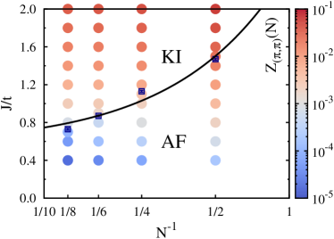
A partial answer to these questions is given in Fig. 1 showing the ground-state phase diagram of the SU($N$) KLM as a function of the inverse of the number of fermion components $N$ and Kondo coupling $J$. Our main result is that the SU($N$) KLM in the fully antisymmetric self-adjoint representation supports magnetic ordering for each considered value of $N$, and that no other phases aside from the Kondo insulator and Néel state intervene, see Secs. IV.1 and  IV.5.

Intuitively, we expect the $J=0$ and $N\rightarrow\infty$ point to be singular. For the ordering of limits $\lim_{N\rightarrow\infty}\lim_{J\rightarrow 0}$ we expect an AF ground state whereas for $\lim_{J\rightarrow 0}\lim_{N\rightarrow\infty}$ we expect a paramagnetic one. Figure 1 confirms this point of view: the magnetic order-disorder transition point (empty squares), extracted from the behavior of the staggered moment Eq. (21) in the thermodynamic limit, shifts upon increasing $N$ to smaller values of $J/t$ which enhances the domain of stability of the KI phase at the expense of the AF state. While the RKKY scale varies as $\frac{1}{N}$, the Kondo scale is $N$ independent such that comparing scales yields an estimate of the critical coupling $J_{c}(N)\propto\frac{1}{\ln{N}}$ in the large-$N$ and small $J$ limit (see Appendix A). We have used this form to plot a guide to the eye for the phase boundary in Fig. 1.

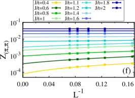
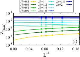
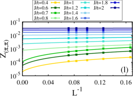
In addition, color-coded circles in Fig. 1 correspond to the QP residue $Z_{\boldsymbol{k}}$ of the doped hole at momentum $(\pi,\pi)$ extrapolated to the thermodynamic limit. We extracted this quantity directly on the imaginary-time axis by fitting the tail of the single-particle Green’s function for conduction electrons to the form $Z_{\boldsymbol{k}}e^{-\Delta_{qp}(\boldsymbol{k})\tau}$ where $\Delta_{qp}$ is the single-particle gap. At $N=2$, and in the magnetically ordered phase, we observe a remarkable coexistence of Kondo screening and antiferromagnetism that stands at odds with the mean-field result predicting only a very narrow coexistence region Zhang and Yu (2000); Capponi and Assaad (2001). We show in Sec. IV.2 that this does not carry over over to larger values of $N$ where we observe an abrupt drop in the QP residue $Z_{(\pi,\pi)}$ across the magnetic transition, see Fig. 1.

Finally, in Secs. IV.3 and IV.4 we investigate the impact of an enhanced Hamiltonian symmetry on the spin excitation spectrum and single-particle spectral function, respectively. We proceed now to discuss numerical results which led us to the above phase diagram.

IV Numerical results

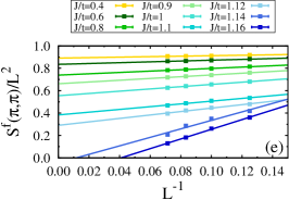
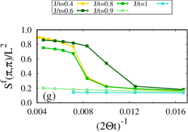
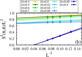
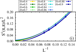
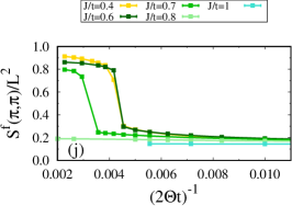
Numerical results were obtained with an $N$-dependent projection parameter ranging from $2\Theta t=50$ for $N=2$ to $2\Theta t=400$ for $N=8$, chosen sufficiently large to guarantee the convergence to the ground state $|\Psi_{0}\rangle$, see Appendix C.1. Physical observables have been extrapolated to the thermodynamic limit based on the QMC data obtained on lattice sizes ranging from $6\times 6$ to $14\times 14$ with periodic boundary conditions. Finite-size scalings and representative raw QMC data are presented in Appendices C.2, C.4, and C.3.

IV.1 Spin degrees of freedom

Figure 2: Staggered moment $m^{\alpha}$ of the: (a) $f$-electrons and (b) $c$-electrons as well as (c) the spin gap $\Delta_{s}$ of the SU($N$) KLM after extrapolation the QMC data to the thermodynamic limit, see Appendices C.2 and C.3. For $N=6$ with $J/t<0.5$ and for $N=8$ for all values of $J$, we were not able to distinguish $m^{c}$ from zero.

We define the Néel state for the SU($N$) quantum antiferromagnet as:

$$|\Psi_{\text{N\'{e}el}}\rangle=\prod_{\boldsymbol{i}\in A}\hat{f}^{\dagger}_{\boldsymbol{i},1}\cdots\hat{f}^{\dagger}_{\boldsymbol{i},N/2}\prod_{\boldsymbol{i}\in B}\hat{f}^{\dagger}_{\boldsymbol{i},N/2+1}\cdots\hat{f}^{\dagger}_{\boldsymbol{i},N}|0\rangle.$$ (18)

For the square lattice, we can split the lattice into two sublattices A and B such that the nearest neighbors of one sublattice belong to the other. For this Néel state, one will show that for $\boldsymbol{i}\neq\boldsymbol{j}$

$$\frac{4}{N}\sum_{\nu,\mu}\langle\Psi_{\text{N\'{e}el}}|\hat{S}^{f,\mu}_{\boldsymbol{j},\nu}\hat{S}^{f,\nu}_{\boldsymbol{i},\mu}|\Psi_{\text{N\'{e}el}}\rangle=e^{i\boldsymbol{Q}\cdot\left(\boldsymbol{i}-\boldsymbol{j}\right)}.$$ (19)

We hence adopt the following definition of the spin-spin correlation function,

$$S^{\alpha}(\boldsymbol{Q})=\frac{4}{N}\frac{1}{L^{2}}\sum_{\boldsymbol{i},\boldsymbol{j},\mu,\nu}e^{i\boldsymbol{Q}\cdot\left(\boldsymbol{i}-\boldsymbol{j}\right)}\langle\hat{S}^{\alpha,\mu}_{\boldsymbol{j},\nu}\hat{S}^{\alpha,\nu}_{\boldsymbol{i},\mu}\rangle,$$ (20)

with $\alpha=c,f$. To pin down the nature of ground state of the SU($N$) KLM, we compute the staggered moment,

$$m^{\alpha}=\sqrt{\lim_{L\to\infty}\frac{S^{\alpha}(\boldsymbol{Q})}{L^{2}}}.$$ (21)

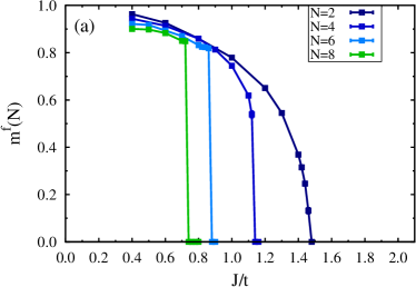
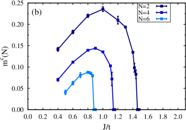
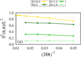
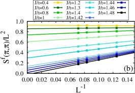
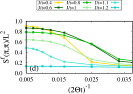
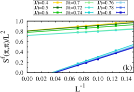
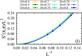
The corresponding finite-size scaling is presented in Appendix C.2 and the extrapolated values for localized (conduction) electrons are plotted versus $J/t$ in Fig. 2(a) [Fig. 2(b)], respectively. On the one hand, the QMC data confirms that increasing $N$ suppresses magnetism by shifting the magnetic order-disorder transition point from $J_{c}/t\simeq 1.47(1)$ in the SU(2) symmetric case to progressively lower values of $J/t$: for $N=4$ we find $J_{c}/t\simeq 1.13(1)$; for $N=6$ and $N=8$ we find the transition points at 0.87(1) and 0.73(1), respectively. In this respect, the effect of finite $N$ bears a similarity to that generated by geometric frustration, e.g., by next-nearest-neighbor hopping $t^{\prime}$ Martin and Assaad (2008); Martin et al. (2010). On the other hand, the data in Fig. 2(a) suggests that in the magnetically ordered phase, the $f$-local moment $m^{f}$ remains large since up to $N=8$ it exceeds 80% of the Néel value. Furthermore, while $m^{f}$ seems to grow continuously below $J_{c}$ at $N=2$, one finds a rapid buildup of the $f$-local moment for larger $N$.

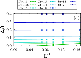
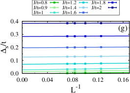
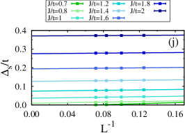
Once the magnetic order disappears at $J_{c}$, the ground state is expected to develop a finite spin gap $\Delta_{s}(\boldsymbol{q})$, i.e., the energy difference between the singlet $S=0$ ground state and the lowest excited spin triplet $S=1$ state with momentum $\boldsymbol{q}$. To compute $\Delta_{s}(\boldsymbol{q})$ without resorting to analytic continuation, we consider the imaginary-time displaced spin correlation functions,

$$S(\boldsymbol{q},\tau)=\sum_{\mu,\nu}\langle\hat{S}^{\mu}_{\nu}(\boldsymbol{q},\tau)\hat{S}^{\nu}_{\mu}(-{\boldsymbol{q}})\rangle,$$ (22)

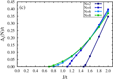
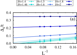
where $\hat{S}^{\mu}_{\nu}(\boldsymbol{q},\tau)=\hat{S}^{f,\mu}_{\nu}(\boldsymbol{q},\tau)+\hat{S}^{c,\mu}_{\nu}(\boldsymbol{q},\tau)$ is the total spin. The spin gap $\Delta_{s}(\boldsymbol{q})$ can be extracted from the asymptotic behavior of $S(\boldsymbol{q},\tau)$ at $\tau t\gg 1$ since $S(\boldsymbol{q},\tau)\propto\exp\left(-\tau\Delta_{s}(\boldsymbol{q})\right)$. Here, we focus on the AF wavevector $\boldsymbol{Q}=(\pi,\pi)$, i.e., $\Delta_{s}\equiv{\rm min}_{\boldsymbol{q}}\Delta_{s}(\boldsymbol{q})=\Delta_{s}(\boldsymbol{Q})$. A linear extrapolation of finite-size QMC estimates of $\Delta_{s}(N)$ to the thermodynamic limit, see Appendix C.3, leads to the results plotted in Fig. 2(c). For each $N$ we find that opening of the spin gap coincides with the vanishing of the magnetic moment. As shown in Fig. 2(c), upon increasing $N$ the $J$-dependence of the spin gap approaches asymptotically the large-$N$ behavior $\propto e^{-t/J}$.

Figure 3: (a) Expectation value of the Kondo interaction term $\hat{\mathcal{H}}_{J}$ corresponding to the derivative of the free energy with respect to $J$ obtained on the $14\times 14$ lattice. The arrows indicate magnetic order-disorder transition points. Bottom panels show a close-up around the transition point: (b) $N=4$, (c) $N=6$, and (d) $N=8$.

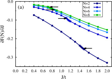
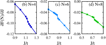
While the spin gap evolves smoothly across the transition, the magnetization shows an abrupt change, especially at larger values of $N$. This poses the question of the nature of the transition, first order or continuous. To provide more insight, we plot in Fig. 3 the free-energy derivative,

$$\frac{\partial F}{\partial J}=\frac{1}{L^{2}}\frac{\langle\hat{\mathcal{H}}_{J}\rangle}{J},$$ (23)

obtained on our largest $14\times 14$ lattice. A progressively steeper evolution of this quantity across the transition point suggests that the phase transition becomes first order upon increasing $N$.

IV.2 Charge degrees of freedom

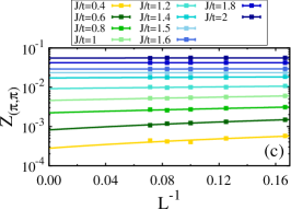
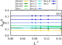
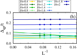
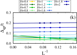
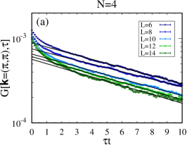
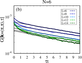
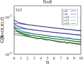
An important quantity of direct experimental relevance is the QP residue $Z_{\boldsymbol{k}}$. Indeed, since the effective QP mass $m^{*}\propto\frac{1}{Z_{\boldsymbol{k}}}$, the behavior of $Z_{\boldsymbol{k}}$ along the Fermi surface reveals how electron interactions modify properties of a metal. Given that QMC simulations are restricted to the half-filled case, one possibility to get insight into properties of the metallic state at small doping is to consider the problem of a single-hole doped into the insulating phase. Then, assuming a rigid band scenario, one can estimate the QP residue $Z_{\boldsymbol{k}}=\left|\langle\Psi_{0}^{n}|c^{\dagger}_{\boldsymbol{k},\sigma}|\Psi_{0}^{n-1}\rangle\right|^{2}$ of the doped hole at momentum $\boldsymbol{k}$ together with the corresponding QP gap $\Delta_{qp}(\boldsymbol{k})=E_{0}^{n}-E_{0}^{n-1}(\boldsymbol{k})$, directly from the long-time behavior of the imaginary-time Green’s function:

$$G(\boldsymbol{k},\tau)=\frac{1}{N}\sum_{\sigma}\langle\Psi_{0}^{n}|c^{\dagger}_{\boldsymbol{k},\sigma}(\tau)c_{\boldsymbol{k},\sigma}|\Psi_{0}^{n}\rangle\stackrel{{\scriptstyle\tau\to\infty}}{{\to}}Z_{\boldsymbol{k}}e^{-\Delta_{qp}(\boldsymbol{k})\tau}.$$ (24)

Here, $E_{0}^{n}$ is the ground-state energy at half-filling with $n$ particles while $E_{0}^{n-1}(\boldsymbol{k})$ corresponds to the energy eigenstate with momentum $\boldsymbol{k}$ in the $n-1$ particle Hilbert space. Typical raw data of $G(\boldsymbol{k},\tau)$ from QMC simulations with different system sizes $L$ and the extrapolation to the thermodynamic limit of finite-size estimates of $\Delta_{qp}\equiv{\rm min}_{\boldsymbol{k}}\Delta_{qp}(\boldsymbol{k})=\Delta_{qp}(\boldsymbol{k}=(\pi,\pi))$ and $Z_{(\pi,\pi)}$ are presented in Appendix C.4.

Figure 4: (a) Single-particle gap $\Delta_{qp}$ at momentum $\boldsymbol{k}=(\pi,\pi)$ and (b) the corresponding QP residue $Z_{(\pi,\pi)}$ after extrapolation the QMC data to the thermodynamic limit, see Appendix C.4. Insets show second-order polynomial fits to the QMC data in order to extract $\Delta_{qp}$ and $Z_{(\pi,\pi)}$ in the $N\to\infty$ limit; the extrapolated values $\Delta_{qp}^{N\to\infty}=0.109(3)$ and $Z_{(\pi,\pi)}^{N\to\infty}=0.0256(3)$ at $J/t=2$ and $\Delta_{qp}^{N\to\infty}=0.051(2)$ and $Z_{(\pi,\pi)}^{N\to\infty}=0.0125(2)$ at $J/t=1.6$ match well those obtained using the large-$N$ approximation (triangles).

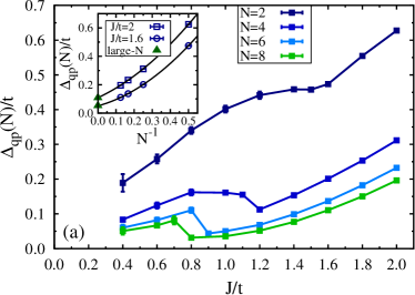
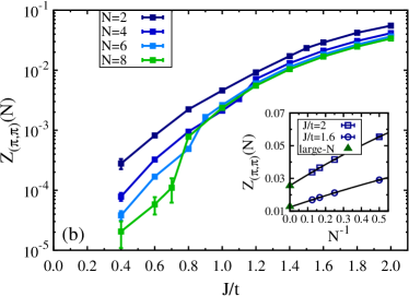
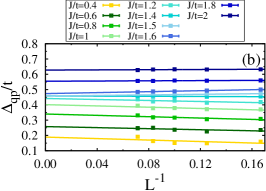
Figure 4 plots $\Delta_{qp}$ and $Z_{(\pi,\pi)}$ as a function of $J/t$. We first discuss the evolution of these quantities in the paramagnetic phase. As shown in the insets of Fig. 4 both quantities evolve smoothly from $N=2$ to $N=\infty$. The fact that we are able to recover the large-$N$ results by extrapolating QMC data obtained by handling the constraint of no double occupancy on the localized $f$-electron orbitals numerically exactly, validates the large-$N$ approximate treatments of the constraint and confirms that the large-$N$ theory is the correct saddle point of the SU(2) KLM. Furthermore, by comparing the $N$-dependence of the single-particle gap $\Delta_{qp}$ in Fig. 4(a) with that of the spin gap $\Delta_{s}$ in Fig. 2(c), we conclude that upon increasing $N$ both quantities evolve in the paramagnetic phase (i.e. $J/t=2$) to the asymptotic limit $\Delta_{s}=\Delta_{c}$ with $\Delta_{c}=2\Delta_{qp}$ being the charge gap, corresponding to the band insulator in the noninteracting periodic Anderson model. Our results hence provide a text-book numerical demonstration that the $N=2$ Kondo lattice in the paramagnetic phase is adiabatically connected to the large-$N$ saddle point.

Across the magnetic transition, $\Delta_{qp}$ and $Z_{(\pi,\pi)}$ show a very strong $N$ dependence. In contrast to the $N=2$ case with a smooth evolution of both quantities across the quantum critical point at $J_{c}/t\simeq 1.47$, a nonmonotonic behavior of the single-particle gap accompanied by an abrupt reduction of the QP weight on the magnetically ordered side is apparent. Although $Z_{(\pi,\pi)}$ shows an abrupt change, it remains finite in the magnetic phase. Hence we find the continued existence of the heavy-fermion band for all the considered values of $N$ down to the smallest $J$. Assuming a rigid-band scenario this implies that, in contrast to an Ansatz with frozen $f$-spins, the emergent heavy-fermion metal at small coupling $J$ is characterized by a large Fermi surface containing both conduction and localized electrons (see Sec. V ). As a consequence, the coherence temperature is expected to drop abruptly across the transition. On the magnetically ordered side, the QP gap tracks $J/N$ in the small $J$ limit. Finally, a notable feature in Fig. 4(a) is a broad plateau in the $J$-dependence of $\Delta_{qp}$ at $N=4$. It is interesting to point out that a similar plateau was found in quantum cluster theories allowing for SU(2) symmetry-breaking AF order Martin et al. (2010); Lenz et al. (2017) as well as in the bond fermion theory Eder and Wróbel (2018).

To provide a theoretical framework for the above, we introduce in Appendix B a mean-field theory. Here we describe how this mean-field theory and fluctuations around the corresponding saddle point can account for the QMC results. Our numerics shows that for any fixed value of $N$ the paramagnetic state is unstable to an RKKY driven magnetic instability and that deep in the magnetic phase the $f$-local moment is next to saturated. The Néel state of Eq. (18) is hence a good starting point to formulate a mean-field theory. This wave function breaks the U($N$) symmetry down to U($N$/2) $\times$ U($N$/2). The mean-field Hamiltonian derived in Appendix B possesses a U($N$/2) $\times$ U($N$/2) symmetry and is a generalization of the mean-field theory of Ref. Zhang and Yu (2000) that captures both Kondo screening and magnetism to the SU($N$) group. In the mean-field Hamiltonian the RKKY interaction scales as $1/N$. As a consequence, and owing to the nesting properties of the conduction-electron band, the magnetically induced QP gap scales as $J/N$. Our QMC results support this.

Following Ref. Assaad et al. (2003) one can define a model Hamiltonian that reduces to the KLM model at $N=2$, that has the U($N$/2) $\times$ U($N$/2) symmetry beyond $N=2$, and that reproduces the saddle point of Eq. (B) in the large-$N$ limit. It is very tempting to interpret our QMC results in terms of fluctuations – that are suppressed as a function of $N$ – around this magnetic saddle point. In the limit $N\rightarrow\infty$ Capponi and Assaad (2001), and deep in the magnetically ordered phase, the $f$-spins are frozen and $Z_{(\pi,\pi)}$ vanishes.

IV.3 Spin excitation spectrum

Figure 5: Dynamical spin structure factor $S(\boldsymbol{q},\omega)$ along a high symmetry path in the Brillouin zone in the: (a-c) AF phase at $J/t=0.8$ and (d-f) KI phase at $J/t=1.6$ obtained on the $14\times 14$ lattice with increasing $N$ (from left to right). In panels (a-c), the particle-hole continuum threshold (dashed) lies above the Goldstone modes $\omega_{\textrm{ph}}/t\simeq 0.68$, 0.32, and 0.22, respectively, while in panels (d-f) it drops from $\omega_{\textrm{ph}}/t\simeq 1$ through $0.4$ to $0.28$.

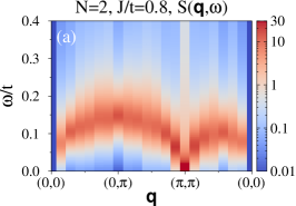
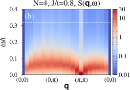
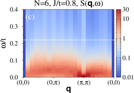
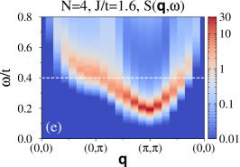
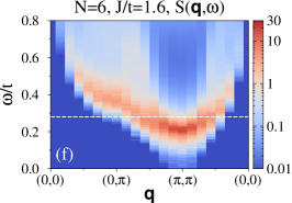
To get further insight into the nature of AF and KI phases in the SU($N$) symmetric situation, we consider the dynamical spin structure factor $S(\boldsymbol{q},\omega)$. We have extracted this quantity from the QMC imaginary-time displaced spin correlation functions defined in Eq. (22),

$$S(\boldsymbol{q},\tau)=\frac{1}{\pi}\int_{0}^{\infty}{\rm d}\omega\;e^{-\tau\omega}S(\boldsymbol{q},\omega),$$ (25)

by using the stochastic analytic continuation method Beach (2004). In the above, we consider the total spin.

The spin-density-wave approximation presented in Appendix B breaks explicitly the SU($N$) symmetry and hence it fails to capture Goldstone modes. Since the Néel state has the U($N/2$) $\times$ U($N/2$) symmetry but the Hamiltonian has a U($N$) one, we expect a total of $\text{dim }\frac{U(N)}{U(N/2)\times U(N/2)}=N^{2}/2$ Goldstone modes Goldstone et al. (1962); Watanabe (2020) that should become apparent in the dynamical spin structure factor. One expects that this large number of Goldstone modes will destabilize the ordering and in this respect, it is interesting to see that in the KLM an AF state can be stabilized for each $N$. Concerning the energetics, and as argued in Appendix A, the effective RKKY coupling $J_{\textrm{RKKY}}$ scales as $\tfrac{J^{2}N(\epsilon_{f})}{N}$ and the single-particle gap as $\tfrac{J}{N}$. Hence in the small $J$ limit, the Goldstone modes are expected to be located well below the particle-hole continuum.

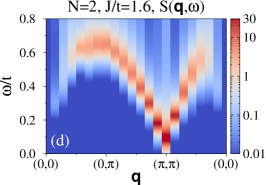
We demonstrate the above in Figs. 5(a-c) where substantial slowing down of the spin-wave velocity $v_{s}\propto J_{\textrm{RKKY}}\sim\tfrac{J^{2}N(\epsilon_{f})}{N}$ in the AF phase with $J/t=0.8$ is clearly seen for $N>2$. For each $N$ considered in Figs. 5(a-c), the particle-hole continuum lies above the Goldstone modes such that we should interpret the data solely in terms of an SU($N$) quantum spin model. Adopting this point of view, the relevant energy scale is the spin-wave velocity that at fixed $J$ scales as $1/N$. In terms of this energy scale, it becomes apparent that the width of the dynamical spin structure factor at say wavevector $\boldsymbol{q}=\left(0,\pi\right)$ grows as a function of $N$. We interpret this as a consequence of scattering between a growing number of Goldstone modes. One should also mention that as a function of growing values of $N$, the distance to the magnetic order-disorder transition point is suppressed. Although for all considered values of parameters the magnetic moment is well developed, this could certainly play a role in the interpretation of the $N$-dependence of the spectrum.

Figures 5(d-f) plot the dynamical spin structure factor at $J/t=1.6$ as a function of $N$. At $N=2$, we are close to the quantum critical point, and the triplon mode shows a minimal gap at the AF wavevector, ${\boldsymbol{Q}}=(\pi,\pi)$. Triplons will condense at the transition to generate the magnetic order. In this regime triplons are bound electron-hole pairs and the binding originates from vertex corrections. Enhancing $N$ from this point, damps vertex corrections such that the bound triplon mode will progressively merge in the particle-hole continuum. Precisely this effect is seen in Figs. 5(d-f).

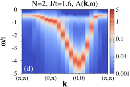
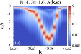
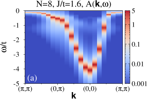
IV.4 Single-particle spectral function

Figure 6: Single-particle spectral function $A(\boldsymbol{k},\omega)$ of the conduction electrons in the: (a-c) AF phase at $J/t=0.8$ and (d-f) KI phase at $J/t=1.6$ obtained on the $14\times 14$ lattice with increasing $N$ (from left to right).

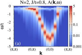
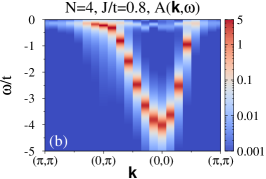
We move on to discuss in more detail the single-particle dynamics. To this end, we have computed the single-particle spectral function $A(\boldsymbol{k},\omega)$ of the conduction electrons. It is related to the imaginary-time Green’s function defined in Eq. (24) via:

$$G(\boldsymbol{k},\tau)=\frac{1}{\pi}\int_{0}^{\infty}{\rm d}\omega\;e^{-\tau\omega}A(\boldsymbol{k},-\omega).$$ (26)

Again, we use the stochastic analytic continuation method to extract $A(\boldsymbol{k},\omega)$.

The evolution of $A(\boldsymbol{k},\omega)$ upon increasing $N$ in the AF phase at $J/t=0.8$ is shown in Figs. 6(a-c). As expected for the half-filled case, all the spectra display a clear hybridization gap which, in agreement with findings in Sec. IV.2, becomes gradually smaller at larger $N$. Furthermore, the spectral function features a flat heavy-fermion band extending to the $\boldsymbol{k}=(\pi,\pi)$ point with relatively low spectral weight. The continued presence of this band around $\boldsymbol{k}=(\pi,\pi)$ even in the AF phase shows that the heavy fermions undergo a magnetic instability such that Kondo screening is still present in the ordered phase.

A direct consequence of the magnetic ordering is a back-folding of the Brillouin zone and the emergence of additional low-energy spectral feature around the $\boldsymbol{k}=(0,0)$ momentum. It arises due to the scattering of the heavy QP off spin fluctuations with the AF wavevector $\boldsymbol{Q}=(\pi,\pi)$ and thus it corresponds to the shadow of the band in the vicinity of the $\boldsymbol{k}=(\pi,\pi)$ point. As apparent, the shadow band becomes less pronounced at larger $N$. This can be traced back to the combined effects that the $Z$-factor at $\boldsymbol{k}=(\pi,\pi)$ drops as a function of $N$ and that the magnetic moment is reduced as $N$ grows from $2$ to $6$ at $J/t=0.8$.

Figure 7: Single-particle spectral function $A(\boldsymbol{k},\omega)$ in the KI phase at $J/t=1.6$ from: (a) QMC simulations with $N=8$ and (b) the large-$N$ approach.

In Figs. 6(d-f) we show the evolution of $A(\boldsymbol{k},\omega)$ upon increasing $N$ in the KI phase at $J/t=1.6$. In the disordered phase with $N=2$, only a precursive feature of the shadow band is visible, see Fig. 6(d): despite a much larger spectral weight of the heavy QP band at $\boldsymbol{k}=(\pi,\pi)$ point with respect to $J/t=0.8$, the precursive feature has relatively low intensity and it is shifted by the energy corresponding roughly to the spin gap $\Delta_{s}$. As shown in Figs. 6(e,f), this feature becomes broad and consequently more difficult to resolve at larger $N$. This can be traced back to the fact that as a function of $N$, the triplon mode approaches the particle-hole continuum broadens, and ultimately disappears.

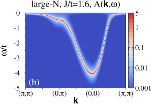
Finally, in Fig. 7 we plot $A(\boldsymbol{k},\omega)$ in the KI phase at $J/t=1.6$ for our largest $N=8$ together with that obtained in the large-$N$ approach. As apparent, the large-$N$ approximation produces a single-particle spectrum which compares favorably with the QMC spectral function. One of the key properties of the large-$N$ self-energy, is its locality:

$$\Sigma(\boldsymbol{k},i\omega_{m})=\frac{(JV)^{2}}{4i\omega_{m}}.$$ (27)

Thereby, despite all the caveats of the large-$N$ approximation – finite hybridization order parameter which breaks the local gauge symmetry – it can be considered to be well suited to account for the essence of Kondo screening deep in the KI phase.

Figure 8: VBS correlation function $S^{f}_{\rm VBS}(\boldsymbol{q})=\sum_{\boldsymbol{\delta}}[S^{f}_{\rm VBS}(\boldsymbol{q})]_{\boldsymbol{\delta},\boldsymbol{\delta}}$ for the $f$-electrons for various lattice sizes measured across the magnetic order-disorder transition point in the: (a,b) AF and (c,d) KI phases for $N=2$ (left) and $N=4$ (right).

Figure 9: Same as in Fig. 8 but for $N=6$ (left) and $N=8$ (right).

IV.5 VBS correlation function

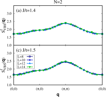
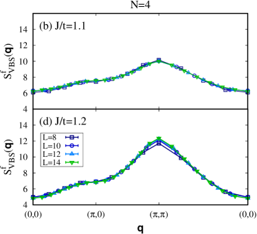
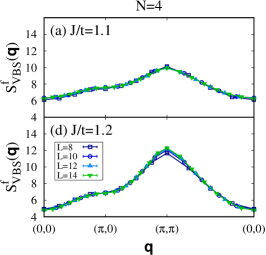
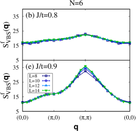
Generically, enhancing the symmetry group from SU(2) to SU($N$) leads to VBS orders. To confirm the absence of this instability in the SU($N$) KLM, we have computed the VBS correlation function for the $f$-spins:

$$\left[S^{f}_{\text{VBS}}(\boldsymbol{q})\right]_{\boldsymbol{\delta},\boldsymbol{\delta^{\prime}}} =\frac{1}{L^{2}}\sum_{\boldsymbol{i},\boldsymbol{j}}e^{i\boldsymbol{q}\cdot\left(\boldsymbol{i}-\boldsymbol{j}\right)}\times$$

$$\left(\langle\hat{\Delta}_{\boldsymbol{i},\boldsymbol{i}+\boldsymbol{\delta}}\hat{\Delta}_{\boldsymbol{j},\boldsymbol{j}+\boldsymbol{\delta^{\prime}}}\rangle-\langle\hat{\Delta}_{\boldsymbol{i},\boldsymbol{i}+\boldsymbol{\delta}}\rangle\langle\hat{\Delta}_{\boldsymbol{j},\boldsymbol{j}+\boldsymbol{\delta^{\prime}}}\rangle\right),$$ (28)

with $\hat{\Delta}_{\boldsymbol{i},\boldsymbol{i}+\boldsymbol{\delta}}=\sum_{\mu,\nu}\hat{S}^{f,\mu}_{\boldsymbol{i},\nu}\hat{S}^{f,\nu}_{\boldsymbol{i}+\boldsymbol{\delta},\mu}$.

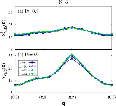
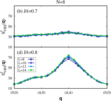
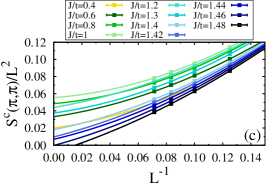
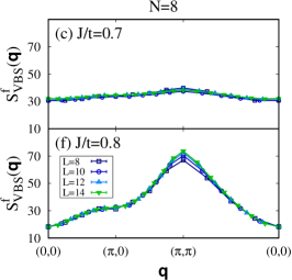
In Fig. 8 we plot this quantity for various lattice sizes along a high symmetry path in the Brillouin zone across the magnetic order-disorder transition for $N=2$ [Figs. 8(a,c)] and $N=4$ [Figs. 8(b,d)]. As expected, the VBS correlation function $S^{f}_{\rm VBS}(\boldsymbol{q})$ for $N=2$ is featureless and lattice-size independent throughout the transition confirming that the SU(2) KLM is dominated by magnetic fluctuations. Given numerical evidence for enhanced columnar ${\boldsymbol{q}}=(\pi,0)$ dimer correlations in SU($N$) Hubbard and Heisenberg models Paramekanti and Marston (2007); Harada et al. (2003); Assaad (2005); Kawashima and Tanabe (2007); Beach et al. (2009); Wang et al. (2014); Okubo et al. (2015); Lang et al. (2013); Zhou et al. (2016, 2017), one could expect that the same physics shows up in the SU($N$) KLM. In contrast, even though the lineshape of $S^{f}_{\rm VBS}(\boldsymbol{q})$ gets sharper at $N=4$, a dominant cusp feature is found at the AF wavevector ${\boldsymbol{Q}}=(\pi,\pi)$, see Figs. 8(b,d). The same behavior is observed across the magnetic order-disorder transition for larger $N=6$ and $N=8$ shown in Figs. 9(a,c) and 9(b,d), respectively. Thus, we conclude that there are no significant columnar dimer fluctuations in the phase diagram and we interpret the cusp feature at ${\boldsymbol{Q}}=(\pi,\pi)$ as a fingerprint of the perfectly nested conduction-electron Fermi surface in the noninteracting limit.

V Discussion

V.1 Experimental relevance

Heavy-fermion systems are prototype materials to study quantum criticality of the magnetic order-disorder transition. Given the complexity of the problem, theoretical and experimental studies on the quantum criticality in heavy-fermion systems explore various routes to approach the quantum critical point (QCP) Löhneysen et al. (2007); Gegenwart et al. (2008); Si and Steglich (2010). One possibility is to modify the strength of the Kondo coupling, e.g., by varying chemical or external pressure. Another route is to tune intersite interactions between the $f$-moments by considering systems with different dimensionality or with geometrical frustration.

In some materials, e.g., Ce_1-xLa_xRu₂Si₂ Knafo et al. (2009), the data are consistent with predictions of the conventional spin-density-wave theory Hertz (1976); Millis (1993), which considers the $f$-electrons as itinerant on both sides of the QCP. In this case, the dominant critical AF fluctuations modify neither the shape nor size of the large Fermi surface which incorporates both conduction electrons and the $f$-electron states. In other compounds such as CeCu_6-xAu_x Schröder et al. (2000) and YbRh₂Si₂ Custers et al. (2003); Paschen et al. (2004); Pfau et al. (2012), there are indications for the breakup of composite heavy-fermion QPs and the concomitant collapse of the large Fermi surface driven by local critical magnetic fluctuations Coleman et al. (2001); Si et al. (2001). Moreover, the reconstruction of the Fermi surface may also occur away from the QCP — within the magnetically ordered phase Custers et al. (2012) or even more exotically — outside Friedemann et al. (2009), paving the way for an intervening phase where the local $f$-moments are neither Kondo screened nor antiferromagnetically ordered.

Here, in order to gain novel insight into the quantum criticality in heavy-fermion systems, we have considered the SU($N$) generalization of the KLM. Given that increasing $N$ changes the degree of quantum fluctuations of the local $f$-moments, it allows one to investigate the impact of magnetic fluctuations on the coherent Kondo-lattice formation in a single setup. Importantly, we do not observe a breakdown of Kondo screening which continues to exist on the magnetically ordered side of the phase diagram. However, our findings show that increasing $N$ strongly modifies the behavior of the QP residue $Z_{(\pi,\pi)}$ across the magnetic phase transition. As such they have important implications for the interpretation of experimental data. Considering that in reality experiments are performed at small but finite temperatures, a rapid decrease of the QP residue resolved for $N=8$, see Fig. 4(b), could be easily mistaken in the isothermal measurement of Hall coefficient as that in Ref. Paschen et al. (2004), as evidence for a collapse of the large Fermi surface at the QCP.

V.2 Quantum-field-theoretic perspective

Throughout the $J$-$N$ plane, the charge degrees of freedom are gapped. Hence charge fluctuations around half-filling – that mix SU($N$) spin representations – will not contribute in the low-energy effective field theory and can be safely omitted. The remaining degree of freedom is an SU($N$) spin in the totally antisymmetric representation corresponding to a Young tableau consisting of a single column and $N$/2 rows. Since we observe AF phases, the low-energy effective model is that of an SU($N$) quantum antiferromagnet:

$$\hat{H}_{eff}=\frac{J}{N}\sum_{\langle\boldsymbol{i},\boldsymbol{j}\rangle,\mu,\nu}\hat{S}^{\mu}_{\boldsymbol{i},\nu}\hat{S}^{\nu}_{\boldsymbol{j},\mu},$$ (29)

in the aforementioned representation. The generalization of Haldane’s SU(2) spin coherent state path integral formulation Haldane (1988) to the SU($N$) group has been carried by Read and Sachdev Read and Sachdev (1989a). It is beyond the scope of this paper to review the derivation, and we will only cite the final result. We consider a square lattice that can be decomposed into two subattices, A and B, such that the nearest neighbors of one sublattice belong to the other. As for the SU(2) case the SU($N$) spin coherent state $|q\rangle$ is obtained by an SU($N$) rotation of the Néel state Perelomov (1972); Read and Sachdev (1989a). It satisfies the relation:

$$\langle q|\hat{S}^{\mu}_{\boldsymbol{i},\nu}|q\rangle=\pm Q^{\mu}_{\nu}(\boldsymbol{i})\equiv\pm\left(\hat{U}^{\dagger}(\boldsymbol{i})\Lambda\hat{U}(\boldsymbol{i})\right)^{\mu}_{\nu}\text{ with }$$

$$\Lambda=\begin{pmatrix}1_{N/2\times N/2}&0\\ 0&-1_{N/2\times N/2}\end{pmatrix},$$ (30)

and the $\pm$ sign refers to the A and B sublattices. $Q^{\mu}_{\nu}(\boldsymbol{i})$ hence corresponds to the Néel order parameter, that owing to the sign convention is uniform in space, and whose low-energy fluctuations are governed by the action:

$$S=S_{B}+S_{NL\sigma},$$ (31)

with Berry phase $S_{B}$ Read and Sachdev (1989a) and non-linear $\sigma$ (NL$\sigma$) model,

$$S_{NL\sigma}=\int d\tau d^{2}{\boldsymbol{x}} \frac{\rho_{s}}{2} \text{Tr}\left( \left[\partial_{\boldsymbol{x}}Q(\boldsymbol{x},\tau)\right]^{2} +\frac{1}{c^{2}}\left[\partial_{\tau}Q(\boldsymbol{x},\tau)\right]^{2}\right).$$ (32)

In the above $\rho_{s}$ corresponds to the spin stiffness and $c$ to the velocity. For the SU(2) case, we can write $Q=\boldsymbol{n}\cdot\boldsymbol{\sigma}$ with $\boldsymbol{n}$ a unit vector and $\boldsymbol{\sigma}$ the vector of Pauli spin matrices. With this parametrization, the above reduces to the well known O(3) NL$\sigma$ model with Berry phase. In contrast to the one-dimensions, smooth space-time variations of the Néel order parameter have a vanishing Berry phase Haldane (1988). For the above U($N$) model, the order parameter manifold corresponds to $\frac{U(N)}{U(N/2)\times U(N/2)}$. Since the second homotopy group of this space is given by $\mathbb{Z}$, skyrmions are well defined, and one can carry over the arguments put forward by Haldane for the SU(2) case. In particular, skyrmion number changing field configurations (hedgehogs) carry a non-trivial Berry phase and quadruple hedgehog insertions carry no Berry phase and hence do not interfere destructively. This suggests that the Hilbert space splits into four distinct classes corresponding to the skyrmion number modulo 4. Proliferation of quadruple hedgehog configurations has been argued to correspond to the VBS state Senthil et al. (2004c) and is the essence of the notion of deconfined quantum criticality.

With this background that links the Berry phase to a four-fold degenerate VBS state and the lack of any $(0,\pm\pi)$ and $(\pm\pi,0)$ singularities in the VBS order parameter across the magnetic order-disorder transition point in the QMC data, see Sec. IV.5, we conclude that the Berry phase can be omitted in the effective field theory. A similar result holds for the SU(2) bilayer Heisenberg model Sandvik and Scalapino (1994); Sandvik et al. (1995); van Duin and Zaanen (1997); Wang et al. (2006). The SU($N$) KLM hence provides a lattice realization of NL$\sigma$ model of Eq. (32). To the best of our knowledge, the critical exponents as well as the very nature of the transition as a function of $N$ are unknown. A $1/N$ expansion study of the critical exponents has been carried out in Ref. Wang et al. (2019) for the general representation corresponding to Young tableau of $m$ ($N-m$) rows and one column on sublattice A (B). As pointed out in the paper Wang et al. (2019), the results require $m/N$ to be a small number and cannot be carried over to the self-conjugate representation where $m=N/2$.

VI Conclusions

Our major findings can be summarized by the following points.

(i) A serious caveat of the large-$N$ approximation is that it introduces a finite hybridization order parameter. It breaks the local gauge symmetry and implies that the constraint of single occupancy on the $f$-sites is fulfilled only on average Burdin et al. (2000). Here, we have handled the constraint of no double occupancy numerically exactly with QMC simulations. By extrapolating finite-$N$ QMC data to the $N\to\infty$ limit, we were able to recover the large-$N$ results in the KI phase. This validates large-$N$ approximate treatments of the constraint and confirms that the large-$N$ theory is the correct saddle point of the SU(2) KLM.

(ii) Up to $N=8$ we observe a magnetically ordered phase. The RKKY interaction scales as $1/N$ and the Kondo energy is $N$-independent such that matching the two energy scales gives $J_{c}(N)\propto\frac{1}{\ln(N)N(\epsilon_{F})}$. This form is consistent with our data. Since the charge degrees of freedom are gapped throughout the phase diagram, the magnetically ordered state should be understood in terms of an SU($N$) quantum antiferromagnet on a bilayer square lattice. Let us consider the representations discussed in Ref. Read and Sachdev (1990), consisting of a Young tableau of $m$ ($N-m$) rows and one column on sublattice A (B). The Néel broken symmetry phase of the model has Lorentz symmetry and accordingly $2Nm-2m^{2}$ Goldstone modes Goldstone et al. (1962); Watanabe (2020). This count matches the dimension of the manifold on which the NL$\sigma$ model of Sec. V.2 is defined. The number of Goldstone modes is a measure of the fluctuations around the Néel state and is maximal for the representation $m=N/2$ considered here. It is hence interesting to compare our result to that of Ref. Kaul (2012) for the SU($N$) bilayer Heisenberg model with nearest-neighbor couplings at $m=1$: at $N=8$ no magnetic ordering is present. To reconcile this apparent contradiction we have to take into account the range of the RKKY interaction. To a first approximation, it is given by the inverse single-particle gap in the KI phase at a value of $J$ just above $J_{c}(N)$. With the above form for $J_{c}(N)$ and large-$N$ form for the single-particle gap, $\Delta_{qp}\propto e^{-\frac{1}{JN(\epsilon_{F})}}$, we find that the range of the RKKY interaction grows as a power of $N$. We believe that this enhanced range of the interaction – very specific to the KLM – is the key to stabilize antiferromagnetism at large $N$.

(iii) We have argued in Sec. V.2 that the Berry phase could be omitted, such that the KLM provides a unique possibility to study the critical phenomena associated with the NL$\sigma$ model of Eq. (32) at $m=N/2$. To the best of our knowledge, and as discussed in Sec. V.2, this universality class has never been studied. Our results suggest however that as a function of $N$, the transition does not sustain a quantum critical point Assaad (1999); Schäfer et al. (2019) and becomes first order. Remarkably for bilayer geometries, choosing the fundamental representation on one sublattice and the adjoint on the other, as in Ref. Kaul (2012), one also observes that for $N=4$ and beyond the order-disorder transition is a first order one.

(iv) Since the range of the RKKY interaction grows as a function of $N$ we expect that the interplay between charge and spin degrees of freedom will become more mean-field-like. In fact, at large $N$ we observe an abrupt reduction of the QP residue $Z_{(\pi,\pi)}$ upon entering the AF phase. This behavior is very reminiscent of that observed in mean-field calculations of the SU(2) KLM that take into account both antiferromagnetism and Kondo screening Capponi and Assaad (2001). Within a rigid band shift assumption to describe the heavy-fermion metallic state at small doping, this means that the coherence temperature drops by up to an order of magnitude across the magnetic transition. Isothermal measurement of the Hall coefficient made below the coherence temperature in the paramagnetic heavy-fermion phase and above it in the magnetically ordered state, would be interpreted as a breakdown of Kondo screening Paschen et al. (2004). Nevertheless, we find the signature of the heavy-fermion band for all the considered values of $N$ down to the smallest $J$. With the aforementioned rigid band shift, the emergent heavy-fermion metal at small coupling $J$ is characterized by a large Fermi surface containing both conduction and localized electrons. In the magnetically ordered phase, back-folding of the Fermi surface accounts for the reduced translation symmetry. This abrupt reduction of $Z_{(\pi,\pi)}$ upon entering the AF phase accompanied by a jump in the free-energy derivative $\frac{\partial F}{\partial J}$ could be interpreted as a sign of a first order transition in the high SU($N$) symmetric case.

Appendix A Energy scales of the SU($\boldsymbol{N}$) KLM

A.1 The RKKY scale

The SU($N$) generalization of the KLM of Eq. (1) reads:

$$\hat{\mathcal{H}}=-t\sum_{\langle\boldsymbol{i},\boldsymbol{j}\rangle,\sigma=1}^{N}\hat{c}^{\dagger}_{\boldsymbol{i},\sigma}\hat{c}_{\boldsymbol{j},\sigma}+\frac{2J}{N}\sum_{\boldsymbol{i},a=1}^{N^{2}-1}\hat{T}^{a,c}_{\boldsymbol{i}}\hat{T}^{a,f}_{\boldsymbol{i}}.$$ (33)

Here,

$$\hat{T}^{a,c}=\hat{\boldsymbol{c}}^{\dagger}T^{a}\hat{\boldsymbol{c}}^{\phantom{\dagger}},\;\;\hat{T}^{a,f}=\hat{\boldsymbol{f}}^{\dagger}T^{a}\hat{\boldsymbol{f}}^{\phantom{\dagger}},$$ (34)

and the $N^{2}-1$ generators of SU($N$) satisfy the normalization condition:

$$\text{Tr}\left[T^{a}T^{b}\right]=\frac{1}{2}\delta_{a,b}.$$ (35)

To estimate the energy scale of the RKKY interaction, we will first consider a single impurity at the origin with a frozen $f$-spin:

$$\hat{\mathcal{H}}=-t\sum_{\langle\boldsymbol{i},\boldsymbol{j}\rangle,\sigma=1}^{N}\hat{c}^{\dagger}_{\boldsymbol{i},\sigma}\hat{c}_{\boldsymbol{j},\sigma}+\frac{2J}{N}\sum_{a=1}^{N^{2}-1}\hat{T}^{a,c}_{\boldsymbol{0}}\langle\hat{T}^{a,f}_{\boldsymbol{0}}\rangle.$$ (36)

Within first order perturbation theory in $J$ the frozen $f$-spin at the origin produces ripples in the spin texture that follow the spin susceptibility of the conduction electrons, $\chi^{c}$,

$$\langle\hat{T}^{a,c}_{\boldsymbol{r}}\rangle=-\frac{2J}{N}\langle\hat{T}^{a,f}_{\boldsymbol{0}}\rangle\chi^{c}(\boldsymbol{r},i\Omega_{m}=0).$$ (37)

Here,

$$\chi^{c}(\boldsymbol{q},i\Omega_{m}=0)=\frac{1}{2L^{2}}\sum_{\boldsymbol{k}}\frac{f(\boldsymbol{k}-\boldsymbol{q})-f(\boldsymbol{k})}{\epsilon(\boldsymbol{k})-\epsilon(\boldsymbol{k}-\boldsymbol{q})},$$ (38)

with $\epsilon(\boldsymbol{k})=-2t\left(\cos(k_{x})+\cos(k_{y})\right)$, $f(\boldsymbol{k})=\frac{1}{1+e^{\beta\epsilon(\boldsymbol{k})}}$ and $\chi^{c}(\boldsymbol{r},i\Omega_{m}=0)=\frac{1}{L^{2}}\sum_{\boldsymbol{q}}e^{-i\boldsymbol{q}\cdot\boldsymbol{r}}\chi^{c}(\boldsymbol{q},i\Omega_{m}=0)$. We now consider a second impurity at position $\boldsymbol{r}$ that Kondo couples to the conduction electrons according to Eq. (33). At the mean-field level, the interaction energy between the two spins, reads:

$$\frac{J}{2N}\langle\hat{T}^{a,c}_{\boldsymbol{r}}\rangle\hat{T}^{a,f}_{\boldsymbol{r}}\equiv-\left(\frac{2J}{N}\right)^{2}\chi^{c}(\boldsymbol{r},i\Omega_{m}=0)\langle\hat{T}^{a,f}_{\boldsymbol{0}}\rangle\hat{T}^{a,f}_{\boldsymbol{r}}.$$ (39)

Comparing the above expression to the RKKY Hamiltonian:

$$\hat{H}_{RKKY}=\frac{1}{2N}\sum_{a,\boldsymbol{r}\neq\boldsymbol{r}^{\prime}}J_{RKKY}(\boldsymbol{r}-\boldsymbol{r}^{\prime})\hat{T}^{a,f}_{\boldsymbol{r}}\hat{T}^{a,f}_{\boldsymbol{r}^{\prime}},$$ (40)

that describes the effective SU($N$) Heisenberg interaction between the impurity spins gives:

$$J_{RKKY}(\boldsymbol{r})=-\frac{8J^{2}}{N}\chi^{c}(\boldsymbol{r},i\Omega_{m}=0).$$ (41)

Hence, the RKKY interaction measured relative to the kinetic energy scales as $\frac{1}{N}$.

A.2 The Kondo scale

In contrast, we now argue that the Kondo scale is $N$-independent in the large-$N$ limit. To formulate the large-$N$ mean-field saddle-point, we use the completeness relation,

$$\sum_{a}T^{a}_{\alpha,\beta}T^{a}_{\alpha^{\prime},\beta^{\prime}}=\frac{1}{2}\left(\delta_{\alpha,\beta^{\prime}}\delta_{\alpha^{\prime},\beta}-\frac{1}{N}\delta_{\alpha,\alpha^{\prime}}\delta_{\beta,\beta^{\prime}}\right),$$ (42)

to show that up to a constant:

$$\hat{\mathcal{H}}=-t\sum_{\langle\boldsymbol{i},\boldsymbol{j}\rangle,\sigma=1}^{N}\hat{c}^{\dagger}_{\boldsymbol{i},\sigma}\hat{c}_{\boldsymbol{j},\sigma}-\frac{J}{2N}\sum_{\boldsymbol{i}}\left(\hat{D}^{\dagger}_{\boldsymbol{i}}\hat{D}^{\phantom{\dagger}}_{\boldsymbol{i}}+\hat{D}^{\phantom{\dagger}}_{\boldsymbol{i}}\hat{D}^{\dagger}_{\boldsymbol{i}}\right),$$ (43)

with,

$$\hat{D}^{\dagger}_{\boldsymbol{i}}=\sum_{\sigma=1}^{N}\hat{c}^{\dagger}_{\boldsymbol{i},\sigma}\hat{f}^{\phantom{\dagger}}_{\boldsymbol{i},\sigma}.$$ (44)

Using the mean-field Ansatz $V=2\langle\hat{D}^{\dagger}_{\boldsymbol{i}}\rangle/N$ and imposing the constraint $\sum_{\sigma=1}^{N}\hat{f}^{\dagger}_{\boldsymbol{i},\sigma}\hat{f}^{\phantom{\dagger}}_{\boldsymbol{i},\sigma}=\frac{N}{2}$ on average yields the gap equation:

$$\frac{2}{J}\Delta=\Delta\int d\epsilon N(\epsilon)\frac{f(\frac{\epsilon}{2}-E)-f(\frac{\epsilon}{2}+E)}{E},$$ (45)

where $\Delta=JV/2$, $E=\sqrt{\left(\frac{\epsilon}{2}\right)^{2}+\Delta^{2}}$, $N(\epsilon)=\frac{1}{L^{2}}\sum_{\boldsymbol{k}}\delta(\epsilon-\epsilon(\boldsymbol{k}))$, and $f$ the Fermi function. For the particle-hole symmetric case considered here, the $f$-electron half-filling constraint is satisfied by symmetry such that no Lagrange multiplier has to be introduced. At the Kondo temperature, $T_{K}$, $\Delta$ vanishes, such that $T_{K}$ is given by:

$$\frac{1}{J}=\int_{0}^{\infty}d\epsilon N(\epsilon)\frac{\tanh\left(\frac{\epsilon}{2k_{B}T_{K}}\right)}{\epsilon}.$$ (46)

In the above, we have used the particle-hole symmetric condition $N(\epsilon)=N(-\epsilon)$. As apparent, the above equation is independent on $N$ such that at the mean-field level, the Kondo temperature does not scale with $N$. Finally we note that for a density of states of width $W$ and in the small $J$ limit,

$$k_{B}T_{K}\propto\frac{eW}{2}e^{-W/J}.$$ (47)

A.3 Functional form of the critical coupling $\boldsymbol{J_{c}(N)}$

We can now compare scales to estimate the the critical value of $J_{c}(N)$ where the Kondo effect gives way to magnetic ordering:

$$\frac{e}{2N(\epsilon_{f})}e^{-1/N(\epsilon_{f})J_{c}}=\frac{8J_{c}^{2}}{N}\chi^{c}.$$ (48)

In the above, we have used $N(\epsilon_{f})=\frac{1}{W}$ for the aforementioned flat density of states, and for instance, considered the value of the spin-susceptibility at a distance given by the lattice spacing. In the large-$N$ limit where we expect $J_{c}$ to be small, we obtain:

$$J_{c}(N)\propto\frac{1}{\ln(N)N(\epsilon_{f})}.$$ (49)

Appendix B Spin-density-wave approach for the SU($\boldsymbol{N}$) KLM

The data presented in the main text suggests that for each $N$ magnetism and Kondo screening coexist, and that in the magnetically ordered phase, the $f$-local moment is large since up to $N=8$ it exceeds 80% of the Néel value. In this appendix, we generalized the mean-field theory of Ref. Zhang and Yu (2000) that captures both Kondo screening and magnetism to the SU($N$) group. To do so, we consider the following explicit form of the SU($N$) generators. For $\alpha>\beta$ included in the set of $\left[1,N\right]$ we consider the $N^{2}-N$ off-diagonal generators:

$$\hat{T}^{x,c,\alpha,\beta}_{\boldsymbol{i}} = \frac{1}{2}\left(\hat{c}^{\dagger}_{\boldsymbol{i},\beta}\hat{c}^{\phantom{\dagger}}_{\boldsymbol{i},\alpha}+\hat{c}^{\dagger}_{\boldsymbol{i},\alpha}\hat{c}^{\phantom{\dagger}}_{\boldsymbol{i},\beta}\right),$$

$$\hat{T}^{y,c,\alpha,\beta}_{\boldsymbol{i}} = \frac{1}{2}\left(i\hat{c}^{\dagger}_{\boldsymbol{i},\beta}\hat{c}^{\phantom{\dagger}}_{\boldsymbol{i},\alpha}-i\hat{c}^{\dagger}_{\boldsymbol{i},\alpha}\hat{c}^{\phantom{\dagger}}_{\boldsymbol{i},\beta}\right),$$ (50)

alongside the $N-1$ diagonal operators:

$$\hat{T}^{z,c,n}_{\boldsymbol{i}}=\frac{1}{\sqrt{2(n+n^{2})}}\left(\sum_{\alpha=1}^{n}\hat{c}^{\dagger}_{\boldsymbol{i},\alpha}\hat{c}^{\phantom{\dagger}}_{\boldsymbol{i},\alpha}-n\hat{c}^{\dagger}_{\boldsymbol{i},n+1}\hat{c}^{\phantom{\dagger}}_{\boldsymbol{i},n+1}\right).$$ (51)

In the above, $n$ runs from $1,\ldots,N-1$. This definition of the SU($N$) generators satisfies the normalization condition of Eq. (35) and similar forms hold for the $f$-electrons. As in Ref. Zhang and Yu (2000), the off-diagonal operators will account for Kondo screening whereas the diagonal ones for magnetism. With the above, the SU($N$) Kondo interaction reads:

$$\hat{H}_{K}=\frac{2J}{N} \sum_{\boldsymbol{i}}\left(\sum_{n=1}^{N-1}\hat{T}^{z,n,c}_{\boldsymbol{i}}\hat{T}^{z,n,f}_{\boldsymbol{i}}+\sum_{\alpha>\beta=1}^{N}\hat{T}^{x,\alpha,\beta,c}_{\boldsymbol{i}}\hat{T}^{x,\alpha,\beta,f}_{\boldsymbol{i}}+\hat{T}^{y,\alpha,\beta,c}_{\boldsymbol{i}}\hat{T}^{y,\alpha,\beta,f}_{\boldsymbol{i}}\right)$$

$$=\frac{2J}{N} \sum_{\boldsymbol{i}}\left(\sum_{n=1}^{N-1}\hat{T}^{z,n,c}_{\boldsymbol{i}}\hat{T}^{z,n,f}_{\boldsymbol{i}}-\frac{1}{4}\sum_{\alpha>\beta=1}^{N}\left(\hat{c}^{\dagger}_{\boldsymbol{i},\alpha}\hat{f}^{\phantom{\dagger}}_{\boldsymbol{i},\alpha}+\hat{f}^{\dagger}_{\boldsymbol{i},\beta}\hat{c}^{\phantom{\dagger}}_{\boldsymbol{i},\beta}\right)^{2}+\left(\hat{c}^{\dagger}_{\boldsymbol{i},\beta}\hat{f}^{\phantom{\dagger}}_{\boldsymbol{i},\beta}+\hat{f}^{\dagger}_{\boldsymbol{i},\alpha}\hat{c}^{\phantom{\dagger}}_{\boldsymbol{i},\alpha}\right)^{2}\right).$$ (52)

To account for the Kondo effect, we adopt the mean-field Ansatz:

$$\langle\hat{c}^{\dagger}_{\boldsymbol{i},\alpha}\hat{f}^{\phantom{\dagger}}_{\boldsymbol{i},\alpha}+\hat{f}^{\dagger}_{\boldsymbol{i},\beta}\hat{c}^{\phantom{\dagger}}_{\boldsymbol{i},\beta}\rangle=\langle\hat{c}^{\dagger}_{\boldsymbol{i},\beta}\hat{f}^{\phantom{\dagger}}_{\boldsymbol{i},\beta}+\hat{f}^{\dagger}_{\boldsymbol{i},\alpha}\hat{c}^{\phantom{\dagger}}_{\boldsymbol{i},\alpha}\rangle=-V.$$ (53)

For the magnetism, it is convenient to carry out an orthogonal transformation of the diagonal operators:

$$\tilde{\hat{T}}^{z,c,m}_{\boldsymbol{i}}=\sum_{n=1}^{N-1}O_{m,n}\hat{T}^{z,c,n}_{\boldsymbol{i}},$$ (54)

such that:

$$\tilde{\hat{T}}^{z,c,1}_{\boldsymbol{i}}=\frac{1}{\sqrt{2N}}\left(\sum_{n=1}^{N/2}\hat{c}^{\dagger}_{\boldsymbol{i},n}\hat{c}^{\phantom{\dagger}}_{\boldsymbol{i},n}-\sum_{n=N/2+1}^{N}\hat{c}^{\dagger}_{\boldsymbol{i},n}\hat{c}^{\phantom{\dagger}}_{\boldsymbol{i},n}\right).$$ (55)

Identical forms hold for the $f$-electrons. In the Néel state,

$$|\Psi_{\text{N\'{e}el}}\rangle=\prod_{\boldsymbol{i}\in A}\hat{f}^{\dagger}_{\boldsymbol{i},1}\cdots\hat{f}^{\dagger}_{\boldsymbol{i},N/2}\prod_{\boldsymbol{i}\in B}\hat{f}^{\dagger}_{\boldsymbol{i},N/2+1}\cdots\hat{f}^{\dagger}_{\boldsymbol{i},N}|0\rangle,$$ (56)

we have,

$$\langle\Psi_{\text{N\'{e}el}}|\tilde{\hat{T}}^{z,f,1}_{\boldsymbol{i}}|\Psi_{\text{N\'{e}el}}\rangle=\frac{\sqrt{N}}{2\sqrt{2}}e^{i\boldsymbol{Q}\cdot\boldsymbol{i}},$$ (57)

with the AF wave vector $\boldsymbol{Q}=\left(\pi,\pi\right)$. This motivates the Ansatz:

$$\langle\tilde{\hat{T}}^{z,f,n}_{\boldsymbol{i}}\rangle=\delta_{n,1}\frac{\sqrt{N}}{2\sqrt{2}}e^{i\boldsymbol{Q}\cdot\boldsymbol{i}}m_{f},$$

$$\langle\tilde{\hat{T}}^{z,c,n}_{\boldsymbol{i}}\rangle=-\delta_{n,1}\frac{\sqrt{N}}{2\sqrt{2}}e^{i\boldsymbol{Q}\cdot\boldsymbol{i}}m_{c}.$$ (58)

The above Ansätze break the U($N$) symmetry down to a U($N$/2) $\times$ U($N$/2) one such that it becomes convenient to introduce the notation:

$$\hat{c}^{\dagger}_{\boldsymbol{i},\mu,\sigma}\equiv\hat{c}^{\dagger}_{\boldsymbol{i},\mu+\frac{1+\sigma}{2}\frac{N}{2}},$$

$$\hat{f}^{\dagger}_{\boldsymbol{i},\mu,\sigma}\equiv\hat{f}^{\dagger}_{\boldsymbol{i},\mu+\frac{1+\sigma}{2}\frac{N}{2}},$$ (59)

with $\mu=1,\ldots,N/2$ and $\sigma=\pm 1$. The mean-field Hamiltonian is then given by:

$$\hat{H}_{MF} =\sum_{\mu=1}^{N/2}\sum_{\boldsymbol{k}\in MBZ,\sigma=\pm 1}\begin{pmatrix}\hat{c}^{\dagger}_{\boldsymbol{k},\mu,\sigma}\\ \hat{c}^{\dagger}_{\boldsymbol{k}+\boldsymbol{Q},\mu,\sigma}\\ \hat{f}^{\dagger}_{\boldsymbol{k},\mu,\sigma}\\ \hat{f}^{\dagger}_{\boldsymbol{k}+\boldsymbol{Q},\mu,\sigma}\end{pmatrix}^{T}$$

$$\times\begin{pmatrix}\epsilon(\boldsymbol{k})&\frac{Jm_{f}\sigma}{2N}&JV\frac{N-1}{N}&0\\ \frac{Jm_{f}\sigma}{2N}&-\epsilon(\boldsymbol{k})&0&JV\frac{N-1}{N}\\ JV\frac{N-1}{N}&0&0&-\frac{Jm_{c}\sigma}{2N}\\ 0&JV\frac{N-1}{N}&-\frac{Jm_{c}\sigma}{2N}&0\end{pmatrix}$$

$$\times\begin{pmatrix}\hat{c}_{\boldsymbol{k},\mu,\sigma}\\ \hat{c}_{\boldsymbol{k}+\boldsymbol{Q},\mu,\sigma}\\ \hat{f}_{\boldsymbol{k},\mu,\sigma}\\ \hat{f}_{\boldsymbol{k}+\boldsymbol{Q},\mu,\sigma}\end{pmatrix}+JL^{2}\left(\frac{m_{c}m_{f}}{4}+V^{2}\frac{N-1}{2}\right).$$

Here, $\epsilon(\boldsymbol{k})=-2t\left(\cos(k_{x})+\cos(k_{y})\right)$ such that $\epsilon(\boldsymbol{k}+\boldsymbol{Q})=-\epsilon(\boldsymbol{k})$ and particle-hole symmetry pins the average $f$-occupation to $N/2$. The saddle-point equations then read:

$$\frac{\partial F}{\partial m_{c}}=\frac{\partial F}{\partial m_{f}}=\frac{\partial F}{\partial V}=0,$$ (61)

with $F=-\frac{1}{\beta}\ln{\text{Tr}e^{-\beta\hat{H}_{MF}}}$. Several comments are in order.

• The underlying particle-hole symmetry pins the $f$-occupation to half-filling such that no Lagrange multiplier is required to enforce this constraint on average.

• Since the $\mu$ index does not appear in the Hamiltonian matrix, the above has a U($N$/2) $\times$ U($N$/2) symmetry that generalizes the U(1) $\times$ U(1) symmetry presented in Refs. Zhang and Yu (2000); Capponi and Assaad (2001). One will notice that at $N=2$ we recover precisely Eq. (45) of Ref. Capponi and Assaad (2001). In this case, and assuming $m_{f}=m_{c}=0$ but $V\neq 0$ as appropriate for the KI phase, one finds the single-particle dispersion relation:

  $$E_{\boldsymbol{k}}^{\pm}=\frac{1}{2}\left[\epsilon(\boldsymbol{k})\pm\sqrt{\epsilon^{2}(\boldsymbol{k})+(JV)^{2}}\right],$$ (62)

  QP gap $\Delta_{qp}=-E^{-}_{\boldsymbol{k}=(\pi,\pi)}$ and residue:

  $$Z_{(\pi,\pi)}=\frac{1}{2}\left[1-\frac{\epsilon(\boldsymbol{k}=(\pi,\pi))}{\sqrt{\epsilon^{2}(\boldsymbol{k}=(\pi,\pi))+(JV)^{2}}}\right],$$ (63)

  for a doped hole away from half-filling. Solving self-consistently the saddle-point equation for the hybridization order parameter $V$ and using the above relations for $\Delta_{qp}$ and $Z_{(\pi,\pi)}$ lead us to the large-$N$ results shown in Figs. 4 and 7(b) in the main text. On the other hand, assuming that the AF order is present $m_{f}\neq 0$ and $m_{c}\neq 0$ and the spin degrees of freedom are frozen such that $V=0$, the corresponding dispersion relation reads:

  $$E^{\pm}_{\boldsymbol{k}}=\pm\sqrt{\epsilon^{2}(\boldsymbol{k})+\left(\frac{Jm_{f}}{2N}\right)^{2}},$$ (64)

  and the QP gap tracks $J/N$ as does the QMC data in Fig. 4(a) in the main text.

• While the magnetic energy scales as order $N^{0}$ the kinetic and hybridization energies scale as order $N$. This can be seen explicitly in the last constant term of Eq. (B) and is consistent with the above discussion of the Kondo and RKKY energy scales. As a consequence, we expect the $J=0$ and $N\rightarrow\infty$ point to be singular. For the ordering of limits $\lim_{N\rightarrow\infty}\lim_{J\rightarrow 0}$ we expect an AF ground state whereas for $\lim_{J\rightarrow 0}\lim_{N\rightarrow\infty}$ a paramagnetic one.

• It is very tempting to follow ideas presented in Ref. Assaad et al. (2003) and to formulate a U($N$/2) $\times$ U($N$/2) field theory that possesses the above mean-field Hamiltonian as a saddle point in the large-$N$ limit and that reproduces the U(2) invariant KLM model at $N=2$. At $N=2$, and in the magnetically ordered phase, we observe a remarkable coexistence of Kondo screening and antiferromagnetism that stands at odds with the mean-field results predicting only a very narrow coexistence region Zhang and Yu (2000); Capponi and Assaad (2001). As a function of $N$, fluctuations around the magnetically ordered saddle point are reduced and we expect a stronger mean-field-like competition between magnetic ordering and Kondo screening. It is very interesting to see that the QMC data supports this line of thought.

Appendix C Supplemental data

Figure 10: (a,d,g,j) Convergence of the spin structure factor $S^{f}(\boldsymbol{Q}=(\pi,\pi))$ for the $f$-electrons at representative values of $J/t$ as a function of the projection parameter $\Theta t$ for the $L=12$ system. Panels (b,e,h,k) and (c,f,i,l) show finite-size extrapolation of the spin structure factor for the $f$- and $c$-electrons, respectively, on approaching the magnetic order-disorder transition point; solid lines are linear and second-order polynomial fits to the QMC data. From top to bottom: $N=2,4,6,\text{and }8$.

Here we provide further details about the QMC simulation results discussed in the main text.

C.1 Convergence to the ground state

In this appendix we check the dependence of the QMC results on the projection parameter $\Theta$. In order to ensure that a given result corresponds to the ground state we have performed test simulations on the $12\times 12$ system at a variety of projection parameters $\Theta$. The energy scales of the KLM, the single-ion Kondo temperature, coherence temperature, and the RKKY scale, they all become smaller on decreasing $J/t$. The calculations become more expensive in the SU($N$) case since as shown in Appendix A, the RKKY scale $\propto\tfrac{1}{N}$. Consequently, increasingly large projection parameters are required to reach the AF ground state and the issue becomes particularly severe for small values of $J$, see Figs. 10(a,d,g,j).

Figure 11: Finite-size extrapolation of the: (a,d,g,j) spin gap $\Delta_{s}$, (b,e,h,k) single-particle gap $\Delta_{qp}$ at momentum $\boldsymbol{k}=(\pi,\pi)$, and (c,f,i,l) QP residue $Z_{(\pi,\pi)}$ at representative values of $J/t$. Solid lines are linear fits to the QMC data. From top to bottom: $N=2,4,6,\text{and }8$.

Figure 12: Imaginary-time Green’s function for conduction electrons at momentum $\boldsymbol{k}=(\pi,\pi)$ obtained from QMC simulations for a given linear system size $L$ at $J/t=0.6$ for: (a) $N=4$, (b) $N=6$, and (c) $N=8$. Finite-size estimates of the single-particle gap $\Delta_{qp}(\boldsymbol{k})$ and QP residue $Z_{\boldsymbol{k}}$ are extracted by fitting the tail of the Green’s function to the form $Z_{\boldsymbol{k}}e^{-\Delta_{qp}(\boldsymbol{k})\tau}$ (solid lines).

Figure 13: VBS correlation function $S^{f}_{\rm VBS}(\boldsymbol{q})=\sum_{\boldsymbol{\delta}}[S^{f}_{\rm VBS}(\boldsymbol{q})]_{\boldsymbol{\delta},\boldsymbol{\delta}}$ for the $f$-electrons for various lattice sizes along a high symmetry path in the Brillouin zone across the magnetic order-disorder transition point in the: (a-c) AF and (d-f) KI phases for increasing $N$ (from left to right). Here, a twice smaller imaginary-time step $\Delta\tau t=0.05$ in the Trotter-Suzuki decomposition in Eq. (9) is used as compared to Figs. 8 and 9.

C.2 Spin structure factor

As discussed in Sec. IV.1, we have estimated the onset of long-range magnetic order from the behavior of the staggered magnetic moment:

$$m^{\alpha}=\sqrt{\lim_{L\to\infty}\frac{S^{\alpha}(\boldsymbol{Q}=(\pi,\pi))}{L^{2}}},$$ (65)

extracted separately for the $f$- and $c$-electrons. The corresponding finite-size scaling analysis of the spin structure factor $S^{\alpha}(\boldsymbol{Q})$ is shown in Figs. 10(b,e,h,k) and 10(c,f,i,l), respectively. Long-range AF order is present when $\lim_{L\to\infty}S^{\alpha}(\boldsymbol{Q})/{L^{2}}$ extrapolates to a finite value.

C.3 Spin gap

In Sec. IV.1, the gap for spin excitations $\Delta_{s}(\boldsymbol{q})$ was obtained by considering the imaginary-time displaced spin correlation functions,

$$S(\boldsymbol{q},\tau)=\sum_{\mu,\nu}\langle\hat{S}^{\mu}_{\nu}(\boldsymbol{q},\tau)\hat{S}^{\nu}_{\mu}(-{\boldsymbol{q}})\rangle,$$ (66)

where $\hat{S}^{\mu}_{\nu}(\boldsymbol{q},\tau)=\hat{S}^{f,\mu}_{\nu}(\boldsymbol{q},\tau)+\hat{S}^{c,\mu}_{\nu}(\boldsymbol{q},\tau)$ is the total spin. The spin gap $\Delta_{s}$ for a given linear system size $L$ has been extracted from the asymptotic behavior of $S(\boldsymbol{Q}=(\pi,\pi),\tau)\propto\exp\left(-\tau\Delta_{s}\right)$ at large imaginary time $\tau$. Extrapolating to the thermodynamic limit, one finds for each $N$ that the spin gap scales to a finite value in the KI phase and vanishes inside the AF state due to the emergence of Goldstone modes of the broken continuous SU($N$) symmetry group, see Figs. 11(a,d,g,j).

C.4 Single-particle dynamics

As described in Sec. IV.2, to probe the single-particle dynamics we have measured the imaginary-time displaced Green’s function for the conduction electrons,

$$G(\boldsymbol{k},\tau)=\frac{1}{N}\sum_{\sigma}\langle\Psi_{0}^{n}|c^{\dagger}_{\boldsymbol{k},\sigma}(\tau)c_{\boldsymbol{k},\sigma}|\Psi_{0}^{n}\rangle.$$ (67)

The single-particle gap $\Delta_{qp}$ at momentum $\boldsymbol{k}=(\pi,\pi)$ and the corresponding QP weight $Z_{(\pi,\pi)}$ were extracted by fitting the tail of the Green’s function to the form $Z_{\boldsymbol{k}}e^{-\Delta_{qp}(\boldsymbol{k})\tau}$. As an example, Fig. 12 shows raw data of $G[\boldsymbol{k}=(\pi,\pi),\tau]$ for $N=4$, 6, and 8 obtained from QMC simulations with different system sizes $L$ at $J/t=0.6$. The good quality of the data allowed us to determine finite-size estimates of $\Delta_{qp}$ and $Z_{(\pi,\pi)}$ directly on the imaginary-time axis. The corresponding extrapolation of both quantities to the thermodynamic limit is performed in Figs. 11(b,e,h,k) and 11(c,f,i,l), respectively. Note the enhanced finite-size effects in vicinity of the magnetic transition point.

C.5 Imaginary-time discretization ${\boldsymbol{\Delta}\tau}$

In Sec. IV.5, we have calculated the VBS correlation function $S^{f}_{\rm VBS}(\boldsymbol{q})$. We used the imaginary-time step $\Delta\tau t=0.1$ in the discrete Trotter-Suzuki decomposition in Eq. (9) which yields an error $\mathcal{O}(\Delta\tau^{2})$. In order to exclude that the cusp feature at the AF wavevector ${\boldsymbol{Q}}=(\pi,\pi)$ is an artifact related to the Trotter-Suzuki decomposition, we have repeated QMC simulations for $N=4$, 6, and 8 with a twice smaller imaginary-time step $\Delta\tau t=0.05$. The corresponding dimer structure factors $S^{f}_{\rm VBS}(\boldsymbol{q})$ shown in Fig. 13 look qualitatively very similar to those in Figs. 8(b,d) and 9 in the main text.

References

- Hewson (1993) A. C. Hewson, The Kondo Problem to Heavy Fermions (Cambridge University Press, Cambridge, 1993).
- Kolesnychenko et al. (2002) O. Y. Kolesnychenko, R. de Kort, M. I. Katsnelson, A. I. Lichtenstein, and H. van Kempen, Real-space imaging of an orbital Kondo resonance on the surface, Nature (London) 415, 507 (2002).
- Borda et al. (2003) L. Borda, G. Zaránd, W. Hofstetter, B. I. Halperin, and J. von Delft, Fermi Liquid State and Spin Filtering in a Double Quantum Dot System, Phys. Rev. Lett. 90, 026602 (2003).
- Choi et al. (2005) M.-S. Choi, R. López, and R. Aguado, Kondo Effect in Carbon Nanotubes, Phys. Rev. Lett. 95, 067204 (2005).
- Galpin et al. (2005) M. R. Galpin, D. E. Logan, and H. R. Krishnamurthy, Quantum phase transition in capacitively coupled double quantum dots, Phys. Rev. Lett. 94, 186406 (2005).
- Sasaki et al. (2004) S. Sasaki, S. Amaha, N. Asakawa, M. Eto, and S. Tarucha, Enhanced Kondo Effect via Tuned Orbital Degeneracy in a Spin Artificial Atom, Phys. Rev. Lett. 93, 017205 (2004).
- Jarillo-Herrero et al. (2005) P. Jarillo-Herrero, J. Kong, H. S. van der Zant, C. Dekker, L. P. Kouwenhoven, and S. De Franceschi, Orbital Kondo effect in carbon nanotubes, Nature (London) 434, 484 (2005).
- Lim et al. (2006) J. S. Lim, M.-S. Choi, M. Y. Choi, R. López, and R. Aguado, Kondo effects in carbon nanotubes: From to symmetry, Phys. Rev. B 74, 205119 (2006).
- Makarovski et al. (2007) A. Makarovski, A. Zhukov, J. Liu, and G. Finkelstein, and Kondo effects in carbon nanotube quantum dots, Phys. Rev. B 75, 241407 (2007).
- Tettamanzi et al. (2012) G. C. Tettamanzi, J. Verduijn, G. P. Lansbergen, M. Blaauboer, M. J. Calderón, R. Aguado, and S. Rogge, Magnetic-Field Probing of an Kondo Resonance in a Single-Atom Transistor, Phys. Rev. Lett. 108, 046803 (2012).
- Keller et al. (2014) A. J. Keller, S. Amasha, I. Weymann, C. P. Moca, I. G. Rau, J. A. Katine, H. Shtrikman, G. Zaránd, and D. Goldhaber-Gordon, Emergent Kondo physics in a spin-charge-entangled double quantum dot, Nat. Phys. 10, 145 (2014).
- Martelli et al. (2019) V. Martelli, A. Cai, E. M. Nica, M. Taupin, A. Prokofiev, C.-C. Liu, H.-H. Lai, R. Yu, K. Ingersent, R. Küchler, A. M. Strydom, D. Geiger, J. Haenel, J. Larrea, Q. Si, and S. Paschen, Sequential localization of a complex electron fluid, Proc. Natl. Acad. Sci. USA 116, 17701 (2019).
- Li et al. (1998) J. Li, W.-D. Schneider, R. Berndt, and B. Delley, Kondo Scattering Observed at a Single Magnetic Impurity, Phys. Rev. Lett. 80, 2893 (1998).
- Madhavan et al. (1998) V. Madhavan, W. Chen, T. Jamneala, M. F. Crommie, and N. S. Wingreen, Tunneling into a Single Magnetic Atom: Spectroscopic Evidence of the Kondo Resonance, Science 280, 567 (1998).
- Manoharan et al. (2000) H. C. Manoharan, C. P. Lutz, and D. M. Eigler, Quantum mirages formed by coherent projection of electronic structure, Nature (London) 403, 512 (2000).
- DiLullo et al. (2012) A. DiLullo, S.-H. Chang, N. Baadji, K. Clark, J.-P. Klöckner, M.-H. Prosenc, S. Sanvito, R. Wiesendanger, G. Hoffmann, and S.-W. Hla, Molecular Kondo Chain, Nano Lett. 12, 3174 (2012).
- Tuerhong et al. (2018) R. Tuerhong, F. Ngassam, S. Watanabe, J. Onoe, M. Alouani, and J.-P. Bucher, Two-Dimensional Organometallic Kondo Lattice with Long-Range Antiferromagnetic Order, J. Phys. Chem. C 122, 20046 (2018).
- Figgins et al. (2019) J. Figgins, L. S. Mattos, W. Mar, Y.-T. Chen, H. C. Manoharan, and D. K. Morr, Quantum engineered Kondo lattices, Nat. Commun. 10, 5588 (2019).
- Moro-Lagares et al. (2019) M. Moro-Lagares, R. Korytár, M. Piantek, R. Robles, N. Lorente, J. I. Pascual, M. R. Ibarra, and D. Serrate, Real space manifestations of coherent screening in atomic scale Kondo lattices, Nat. Commun. 10, 2211 (2019).
- Choi et al. (2019) D.-J. Choi, N. Lorente, J. Wiebe, K. von Bergmann, A. F. Otte, and A. J. Heinrich, Colloquium: Atomic spin chains on surfaces, Rev. Mod. Phys. 91, 041001 (2019).
- Khajetoorians et al. (2019) A. A. Khajetoorians, D. Wegner, A. F. Otte, and I. Swart, Creating designer quantum states of matter atom-by-atom, Nat. Rev. Phys. 1, 703 (2019).
- Morr (2017) D. K. Morr, Theory of scanning tunneling spectroscopy: from Kondo impurities to heavy fermion materials, Rep. Prog. Phys. 80, 014502 (2017).
- Raczkowski and Assaad (2019) M. Raczkowski and F. F. Assaad, Emergent Coherent Lattice Behavior in Kondo Nanosystems, Phys. Rev. Lett. 122, 097203 (2019).
- Jiang (2019) M. Jiang, Tunable magnetism of a hexagonal Anderson droplet on the triangular lattice, Phys. Rev. B 100, 014422 (2019).
- Minamitani et al. (2012) E. Minamitani, N. Tsukahara, D. Matsunaka, Y. Kim, N. Takagi, and M. Kawai, Symmetry-Driven Novel Kondo Effect in a Molecule, Phys. Rev. Lett. 109, 086602 (2012).
- Tsukahara et al. (2011) N. Tsukahara, S. Shiraki, S. Itou, N. Ohta, N. Takagi, and M. Kawai, Evolution of Kondo Resonance from a Single Impurity Molecule to the Two-Dimensional Lattice, Phys. Rev. Lett. 106, 187201 (2011).
- Lobos et al. (2014) A. M. Lobos, M. Romero, and A. A. Aligia, Spectral evolution of the Kondo effect from the single impurity to the two-dimensional limit, Phys. Rev. B 89, 121406 (2014).
- Coqblin and Schrieffer (1969) B. Coqblin and J. R. Schrieffer, Exchange Interaction in Alloys with Cerium Impurities, Phys. Rev. 185, 847 (1969).
- Read and Newns (1983) N. Read and D. M. Newns, On the solution of the Coqblin-Schreiffer Hamiltonian by the large-N expansion technique, J. Phys. C 16, 3273 (1983).
- Otsuki et al. (2007) J. Otsuki, H. Kusunose, P. Werner, and Y. Kuramoto, Continuous-Time Quantum Monte Carlo Method for the Coqblin-Schrieffer Model, J. Phys. Soc. Jpn. 76, 114707 (2007).
- Cazalilla and Rey (2014) M. Cazalilla and A. Rey, Ultracold Fermi gases with emergent symmetry, Rep. Prog. Phys. 77, 124401 (2014).
- Foss-Feig et al. (2010a) M. Foss-Feig, M. Hermele, and A. M. Rey, Probing the Kondo lattice model with alkaline-earth-metal atoms, Phys. Rev. A 81, 051603 (2010a).
- Foss-Feig et al. (2010b) M. Foss-Feig, M. Hermele, V. Gurarie, and A. M. Rey, Heavy fermions in an optical lattice, Phys. Rev. A 82, 053624 (2010b).
- Gorshkov et al. (2010) A. V. Gorshkov, M. Hermele, V. Gurarie, C. Xu, P. S. Julienne, J. Ye, P. Zoller, E. Demler, M. D. Lukin, and A. M. Rey, Two-orbital magnetism with ultracold alkaline-earth atoms, Nat. Phys. 6, 289 (2010).
- Zhang et al. (2014) X. Zhang, M. Bishof, S. L. Bromley, C. V. Kraus, M. S. Safronova, P. Zoller, A. M. Rey, and J. Ye, Spectroscopic observation of -symmetric interactions in Sr orbital magnetism, Science 345, 1467 (2014).
- Scazza et al. (2014) F. Scazza, C. Hofrichter, M. Höfer, P. C. De Groot, I. Bloch, and S. Fölling, Observation of two-orbital spin-exchange interactions with ultracold -symmetric fermions, Nat. Phys. 10, 779 (2014).
- Cappellini et al. (2014) G. Cappellini, M. Mancini, G. Pagano, P. Lombardi, L. Livi, M. Siciliani de Cumis, P. Cancio, M. Pizzocaro, D. Calonico, F. Levi, C. Sias, J. Catani, M. Inguscio, and L. Fallani, Direct Observation of Coherent Interorbital Spin-Exchange Dynamics, Phys. Rev. Lett. 113, 120402 (2014).
- Riegger et al. (2018) L. Riegger, N. Darkwah Oppong, M. Höfer, D. R. Fernandes, I. Bloch, and S. Fölling, Localized Magnetic Moments with Tunable Spin Exchange in a Gas of Ultracold Fermions, Phys. Rev. Lett. 120, 143601 (2018).
- Nakagawa and Kawakami (2015) M. Nakagawa and N. Kawakami, Laser-Induced Kondo Effect in Ultracold Alkaline-Earth Fermions, Phys. Rev. Lett. 115, 165303 (2015).
- Kuzmenko et al. (2016) I. Kuzmenko, T. Kuzmenko, Y. Avishai, and G.-B. Jo, Coqblin-Schrieffer model for an ultracold gas of ytterbium atoms with metastable state, Phys. Rev. B 93, 115143 (2016).
- Zhang et al. (2016) R. Zhang, D. Zhang, Y. Cheng, W. Chen, P. Zhang, and H. Zhai, Kondo effect in alkaline-earth-metal atomic gases with confinement-induced resonances, Phys. Rev. A 93, 043601 (2016).
- Cheng et al. (2017) Y. Cheng, R. Zhang, P. Zhang, and H. Zhai, Enhancing Kondo coupling in alkaline-earth-metal atomic gases with confinement-induced resonances in mixed dimensions, Phys. Rev. A 96, 063605 (2017).
- Yao et al. (2019) J. Yao, H. Zhai, and R. Zhang, Efimov-enhanced Kondo effect in alkali-metal and alkaline-earth-metal atomic gas mixtures, Phys. Rev. A 99, 010701 (2019).
- Isaev and Rey (2015) L. Isaev and A. M. Rey, Heavy-Fermion Valence-Bond Liquids in Ultracold Atoms: Cooperation of the Kondo Effect and Geometric Frustration, Phys. Rev. Lett. 115, 165302 (2015).
- Zhong et al. (2017) Y. Zhong, Y. Liu, and H.-G. Luo, Simulating heavy fermion physics in optical lattice: Periodic Anderson model with harmonic trapping potential, Front. Phys. 12, 127502 (2017).
- Caro et al. (2018) R. C. Caro, R. Franco, and J. Silva-Valencia, Spin-liquid state in an inhomogeneous periodic Anderson model, Phys. Rev. A 97, 023630 (2018).
- Ono et al. (2019) K. Ono, J. Kobayashi, Y. Amano, K. Sato, and Y. Takahashi, Antiferromagnetic interorbital spin-exchange interaction of , Phys. Rev. A 99, 032707 (2019).
- Doniach (1977) S. Doniach, The Kondo lattice and weak antiferromagnetism, Physica B+C 91, 231 (1977).
- Tsunetsugu et al. (1997) H. Tsunetsugu, M. Sigrist, and K. Ueda, The ground-state phase diagram of the one-dimensional Kondo lattice model, Rev. Mod. Phys. 69, 809 (1997).
- Löhneysen et al. (2007) H. v. Löhneysen, A. Rosch, M. Vojta, and P. Wölfle, Fermi-liquid instabilities at magnetic quantum phase transitions, Rev. Mod. Phys. 79, 1015 (2007).
- Gegenwart et al. (2008) P. Gegenwart, Q. Si, and F. Steglich, Quantum criticality in heavy-fermion metals, Nat. Phys. 4, 186 (2008).
- Si and Steglich (2010) Q. Si and F. Steglich, Heavy Fermions and Quantum Phase Transitions, Science 329, 1161 (2010).
- Hertz (1976) J. A. Hertz, Quantum critical phenomena, Phys. Rev. B 14, 1165 (1976).
- Millis (1993) A. J. Millis, Effect of a nonzero temperature on quantum critical points in itinerant fermion systems, Phys. Rev. B 48, 7183 (1993).
- Coleman and Nevidomskyy (2010) P. Coleman and A. H. Nevidomskyy, Frustration and the Kondo Effect in Heavy Fermion Materials, J. Low Temp. Phys. 161, 182 (2010).
- Wirth and Steglich (2016) S. Wirth and F. Steglich, Exploring heavy fermions from macroscopic to microscopic length scales, Nat. Rev. Mat. 1, 16051 (2016).
- Coleman et al. (2001) P. Coleman, C. Pépin, Q. Si, and R. Ramazashvili, How do Fermi liquids get heavy and die? J. Phys.: Condens. Matter 13, R723 (2001).
- Si et al. (2001) Q. Si, S. Rabello, K. Ingersent, and J. L. Smith, Locally critical quantum phase transitions in strongly correlated metals, Nature (London) 413, 804 (2001).
- Burdin et al. (2002) S. Burdin, D. R. Grempel, and A. Georges, Heavy-fermion and spin-liquid behavior in a Kondo lattice with magnetic frustration, Phys. Rev. B 66, 045111 (2002).
- Senthil et al. (2003) T. Senthil, S. Sachdev, and M. Vojta, Fractionalized Fermi Liquids, Phys. Rev. Lett. 90, 216403 (2003).
- Senthil et al. (2004a) T. Senthil, M. Vojta, and S. Sachdev, Weak magnetism and non-Fermi liquids near heavy-fermion critical points, Phys. Rev. B 69, 035111 (2004a).
- Motome et al. (2010) Y. Motome, K. Nakamikawa, Y. Yamaji, and M. Udagawa, Partial Kondo Screening in Frustrated Kondo Lattice Systems, Phys. Rev. Lett. 105, 036403 (2010).
- Pixley et al. (2014) J. H. Pixley, R. Yu, and Q. Si, Quantum Phases of the Shastry-Sutherland Kondo Lattice: Implications for the Global Phase Diagram of Heavy-Fermion Metals, Phys. Rev. Lett. 113, 176402 (2014).
- Sato et al. (2018) T. Sato, F. F. Assaad, and T. Grover, Quantum Monte Carlo Simulation of Frustrated Kondo Lattice Models, Phys. Rev. Lett. 120, 107201 (2018).
- Haldane (1988) F. D. M. Haldane, Nonlinear Model and the Topological Distinction between Integer- and Half-Integer-Spin Antiferromagnets in Two Dimensions, Phys. Rev. Lett. 61, 1029 (1988).
- Read and Sachdev (1989a) N. Read and S. Sachdev, Some features of the phase diagram of the square lattice antiferromagnet, Nucl. Phys. B 316, 609 (1989a).
- Read and Sachdev (1989b) N. Read and S. Sachdev, Valence-bond and spin-Peierls ground states of low-dimensional quantum antiferromagnets, Phys. Rev. Lett. 62, 1694 (1989b).
- Read and Sachdev (1990) N. Read and S. Sachdev, Spin-Peierls, valence-bond solid, and Néel ground states of low-dimensional quantum antiferromagnets, Phys. Rev. B 42, 4568 (1990).
- Paramekanti and Marston (2007) A. Paramekanti and J. B. Marston, quantum spin models: a variational wavefunction study, J. Phys.: Condens. Matter 19, 125215 (2007).
- Harada et al. (2003) K. Harada, N. Kawashima, and M. Troyer, Néel and Spin-Peierls Ground States of Two-Dimensional Quantum Antiferromagnets, Phys. Rev. Lett. 90, 117203 (2003).
- Assaad (2005) F. F. Assaad, Phase diagram of the half-filled two-dimensional Hubbard-Heisenberg model: A quantum Monte Carlo study, Phys. Rev. B 71, 075103 (2005).
- Kawashima and Tanabe (2007) N. Kawashima and Y. Tanabe, Ground States of the Heisenberg Model, Phys. Rev. Lett. 98, 057202 (2007).
- Beach et al. (2009) K. S. D. Beach, F. Alet, M. Mambrini, and S. Capponi, Heisenberg model on the square lattice: A continuous- quantum Monte Carlo study, Phys. Rev. B 80, 184401 (2009).
- Wang et al. (2014) D. Wang, Y. Li, Z. Cai, Z. Zhou, Y. Wang, and C. Wu, Competing Orders in the 2D Half-Filled Hubbard Model through the Pinning-Field Quantum Monte Carlo Simulations, Phys. Rev. Lett. 112, 156403 (2014).
- Okubo et al. (2015) T. Okubo, K. Harada, J. Lou, and N. Kawashima, Heisenberg model with multicolumn representations, Phys. Rev. B 92, 134404 (2015).
- Lang et al. (2013) T. C. Lang, Z. Y. Meng, A. Muramatsu, S. Wessel, and F. F. Assaad, Dimerized Solids and Resonating Plaquette Order in -Dirac Fermions, Phys. Rev. Lett. 111, 066401 (2013).
- Zhou et al. (2016) Z. Zhou, D. Wang, Z. Y. Meng, Y. Wang, and C. Wu, Mott insulating states and quantum phase transitions of correlated Dirac fermions, Phys. Rev. B 93, 245157 (2016).
- Zhou et al. (2017) Z. Zhou, D. Wang, C. Wu, and Y. Wang, Finite-temperature valence-bond-solid transitions and thermodynamic properties of interacting Dirac fermions, Phys. Rev. B 95, 085128 (2017).
- Lou et al. (2009) J. Lou, A. W. Sandvik, and N. Kawashima, Antiferromagnetic to valence-bond-solid transitions in two-dimensional Heisenberg models with multispin interactions, Phys. Rev. B 80, 180414 (2009).
- Kaul and Sandvik (2012) R. K. Kaul and A. W. Sandvik, Lattice Model for the Néel to Valence-Bond Solid Quantum Phase Transition at Large , Phys. Rev. Lett. 108, 137201 (2012).
- Block et al. (2013) M. S. Block, R. G. Melko, and R. K. Kaul, Fate of Fixed Points with Monopoles, Phys. Rev. Lett. 111, 137202 (2013).
- Harada et al. (2013) K. Harada, T. Suzuki, T. Okubo, H. Matsuo, J. Lou, H. Watanabe, S. Todo, and N. Kawashima, Possibility of deconfined criticality in Heisenberg models at small , Phys. Rev. B 88, 220408 (2013).
- Senthil et al. (2004b) T. Senthil, A. Vishwanath, L. Balents, S. Sachdev, and M. P. A. Fisher, Deconfined Quantum Critical Points, Science 303, 1490 (2004b).
- Senthil et al. (2004c) T. Senthil, L. Balents, S. Sachdev, A. Vishwanath, and M. P. A. Fisher, Quantum criticality beyond the Landau-Ginzburg-Wilson paradigm, Phys. Rev. B 70, 144407 (2004c).
- Kaul (2012) R. K. Kaul, Quantum phase transitions in bilayer antiferromagnets, Phys. Rev. B 85, 180411 (2012).
- Sandvik and Scalapino (1994) A. W. Sandvik and D. J. Scalapino, Order-disorder transition in a two-layer quantum antiferromagnet, Phys. Rev. Lett. 72, 2777 (1994).
- Sandvik et al. (1995) A. W. Sandvik, A. V. Chubukov, and S. Sachdev, Quantum critical behavior in a two-layer antiferromagnet, Phys. Rev. B 51, 16483 (1995).
- van Duin and Zaanen (1997) C. N. A. van Duin and J. Zaanen, Origin of the Quantum-Critical Transition in the Bilayer Heisenberg Model, Phys. Rev. Lett. 78, 3019 (1997).
- Wang et al. (2006) L. Wang, K. S. D. Beach, and A. W. Sandvik, High-precision finite-size scaling analysis of the quantum-critical point of Heisenberg antiferromagnetic bilayers, Phys. Rev. B 73, 014431 (2006).
- Tahvildar-Zadeh et al. (1998) A. N. Tahvildar-Zadeh, M. Jarrell, and J. K. Freericks, Low-Temperature Coherence in the Periodic Anderson Model: Predictions for Photoemission of Heavy Fermions, Phys. Rev. Lett. 80, 5168 (1998).
- Gröber and Eder (1998) C. Gröber and R. Eder, Temperature-dependent band structure of the Kondo insulator, Phys. Rev. B 57, R12659 (1998).
- Pruschke et al. (2000) T. Pruschke, R. Bulla, and M. Jarrell, Low-energy scale of the periodic Anderson model, Phys. Rev. B 61, 12799 (2000).
- Costi and Manini (2002) T. A. Costi and N. Manini, Low-Energy Scales and Temperature-Dependent Photoemission of Heavy Fermions, J. Low Temp. Phys. 126, 835 (2002).
- Assaad (2004) F. F. Assaad, Coherence scale of the two-dimensional Kondo lattice model, Phys. Rev. B 70, 020402 (2004).
- Yang et al. (2008) Y.-f. Yang, Z. Fisk, H.-O. Lee, J. D. Thompson, and D. Pines, Scaling the Kondo lattice, Nature (London) 454, 611 (2008).
- Raczkowski et al. (2010) M. Raczkowski, P. Zhang, F. F. Assaad, T. Pruschke, and M. Jarrell, Phonons and the coherence scale of models of heavy fermions, Phys. Rev. B 81, 054444 (2010).
- Tanasković et al. (2011) D. Tanasković, K. Haule, G. Kotliar, and V. Dobrosavljević, Phase diagram, energy scales, and nonlocal correlations in the Anderson lattice model, Phys. Rev. B 84, 115105 (2011).
- Kang et al. (2019) H. Kang, K. Haule, G. Kotliar, P. Coleman, and J.-H. Shim, Energy scales of the doped Anderson lattice model, Phys. Rev. B 99, 165115 (2019).
- Costa et al. (2019) N. C. Costa, T. Mendes-Santos, T. Paiva, N. J. Curro, R. R. dos Santos, and R. T. Scalettar, Coherence temperature in the diluted periodic Anderson model, Phys. Rev. B 99, 195116 (2019).
- Burdin et al. (2000) S. Burdin, A. Georges, and D. R. Grempel, Coherence Scale of the Kondo Lattice, Phys. Rev. Lett. 85, 1048 (2000).
- Coleman (1983) P. Coleman, expansion for the Kondo lattice, Phys. Rev. B 28, 5255 (1983).
- Read et al. (1984) N. Read, D. M. Newns, and S. Doniach, Stability of the Kondo lattice in the large- limit, Phys. Rev. B 30, 3841 (1984).
- Auerbach and Levin (1986) A. Auerbach and K. Levin, Kondo Bosons and the Kondo Lattice: Microscopic Basis for the Heavy Fermi Liquid, Phys. Rev. Lett. 57, 877 (1986).
- Millis and Lee (1987) A. J. Millis and P. A. Lee, Large-orbital-degeneracy expansion for the lattice Anderson model, Phys. Rev. B 35, 3394 (1987).
- Coleman et al. (2000) P. Coleman, C. Pépin, and A. M. Tsvelik, Supersymmetric spin operators, Phys. Rev. B 62, 3852 (2000).
- Rech et al. (2006) J. Rech, P. Coleman, G. Zarand, and O. Parcollet, Schwinger Boson Approach to the Fully Screened Kondo Model, Phys. Rev. Lett. 96, 016601 (2006).
- Nilsson (2011) J. Nilsson, Fermionic representations of the Kondo lattice model, Phys. Rev. B 83, 235103 (2011).
- Sykora and Becker (2013) S. Sykora and K. W. Becker, Heavy fermion properties of the Kondo lattice model, Sci. Rep. 3, 2691 (2013).
- Sykora and Becker (2018) S. Sykora and K. W. Becker, Many-body approach to Luttinger’s theorem for the Kondo lattice, Phys. Rev. B 98, 245139 (2018).
- Bercx et al. (2017) M. Bercx, F. Goth, J. S. Hofmann, and F. F. Assaad, The ALF (Algorithms for Lattice Fermions) project release 1.0. Documentation for the auxiliary field quantum Monte Carlo code, SciPost Phys. 3, 013 (2017).
- Assaad (1999) F. F. Assaad, Quantum Monte Carlo Simulations of the Half-Filled Two-Dimensional Kondo Lattice Model, Phys. Rev. Lett. 83, 796 (1999).
- Capponi and Assaad (2001) S. Capponi and F. F. Assaad, Spin and charge dynamics of the ferromagnetic and antiferromagnetic two-dimensional half-filled Kondo lattice model, Phys. Rev. B 63, 155114 (2001).
- Rice and Ueda (1985) T. M. Rice and K. Ueda, Gutzwiller Variational Approximation to the Heavy-Fermion Ground State of the Periodic Anderson Model, Phys. Rev. Lett. 55, 995 (1985).
- Watanabe and Ogata (2007) H. Watanabe and M. Ogata, Fermi-Surface Reconstruction without Breakdown of Kondo Screening at the Quantum Critical Point, Phys. Rev. Lett. 99, 136401 (2007).
- Martin and Assaad (2008) L. C. Martin and F. F. Assaad, Evolution of the Fermi Surface across a Magnetic Order-Disorder Transition in the Two-Dimensional Kondo Lattice Model: A Dynamical Cluster Approach, Phys. Rev. Lett. 101, 066404 (2008).
- Lanatà et al. (2008) N. Lanatà, P. Barone, and M. Fabrizio, Fermi-surface evolution across the magnetic phase transition in the Kondo lattice model, Phys. Rev. B 78, 155127 (2008).
- Vojta (2008) M. Vojta, From itinerant to local-moment antiferromagnetism in Kondo lattices: Adiabatic continuity versus quantum phase transitions, Phys. Rev. B 78, 125109 (2008).
- Hackl and Vojta (2008) A. Hackl and M. Vojta, Kondo volume collapse, Kondo breakdown, and Fermi surface transitions in heavy-fermion metals, Phys. Rev. B 77, 134439 (2008).
- Otsuki et al. (2009) J. Otsuki, H. Kusunose, and Y. Kuramoto, Evolution of a Large Fermi Surface in the Kondo Lattice, Phys. Rev. Lett. 102, 017202 (2009).
- Martin et al. (2010) L. C. Martin, M. Bercx, and F. F. Assaad, Fermi surface topology of the two-dimensional Kondo lattice model: Dynamical cluster approximation approach, Phys. Rev. B 82, 245105 (2010).
- Benlagra et al. (2011) A. Benlagra, T. Pruschke, and M. Vojta, Finite-temperature spectra and quasiparticle interference in Kondo lattices: From light electrons to coherent heavy quasiparticles, Phys. Rev. B 84, 195141 (2011).
- Asadzadeh et al. (2013) M. Z. Asadzadeh, F. Becca, and M. Fabrizio, Variational Monte Carlo approach to the two-dimensional Kondo lattice model, Phys. Rev. B 87, 205144 (2013).
- Peters and Kawakami (2015) R. Peters and N. Kawakami, Large and small Fermi-surface spin density waves in the Kondo lattice model, Phys. Rev. B 92, 075103 (2015).
- Lenz et al. (2017) B. Lenz, R. Gezzi, and S. R. Manmana, Variational cluster approach to superconductivity and magnetism in the Kondo lattice model, Phys. Rev. B 96, 155119 (2017).
- Zhang and Yu (2000) G.-M. Zhang and L. Yu, Kondo singlet state coexisting with antiferromagnetic long-range order: A possible ground state for Kondo insulators, Phys. Rev. B 62, 76 (2000).
- Eder and Wróbel (2018) R. Eder and P. Wróbel, Antiferromagnetic phase of the Kondo insulator, Phys. Rev. B 98, 245125 (2018).
- Assaad et al. (2003) F. F. Assaad, V. Rousseau, F. Hebert, M. Feldbacher, and G. G. Batrouni, Spin and charge dynamics of stripes in doped Mott insulators, Europhys. Lett. 63, 569 (2003).
- Beach (2004) K. S. D. Beach, Identifying the maximum entropy method as a special limit of stochastic analytic continuation, arXiv e-prints (2004), cond-mat/0403055 .
- Goldstone et al. (1962) J. Goldstone, A. Salam, and S. Weinberg, Broken Symmetries, Phys. Rev. 127, 965 (1962).
- Watanabe (2020) H. Watanabe, Counting Rules of Nambu–Goldstone Modes, Annu. Rev. Condens. Matter Phys. 11, 169 (2020).
- Knafo et al. (2009) W. Knafo, S. Raymond, P. Lejay, and J. Flouquet, Antiferromagnetic criticality at a heavy-fermion quantum phase transition, Nat. Phys. 5, 753 (2009).
- Schröder et al. (2000) A. Schröder, G. Aeppli, R. Coldea, M. Adams, O. Stockert, H. v. Löhneysen, E. Bucher, R. Ramazashvili, and P. Coleman, Onset of antiferromagnetism in heavy-fermion metals, Nature (London) 407, 351 (2000).
- Custers et al. (2003) J. Custers, P. Gegenwart, H. Wilhelm, K. Neumaier, Y. Tokiwa, O. Trovarelli, C. Geibel, F. Steglich, C. Pépin, and P. Coleman, The break-up of heavy electrons at a quantum critical point, Nature (London) 424, 524 (2003).
- Paschen et al. (2004) S. Paschen, T. Lühmann, S. Wirth, P. Gegenwart, O. Trovarelli, C. Geibel, F. Steglich, P. Coleman, and Q. Si, Hall-effect evolution across a heavy-fermion quantum critical point, Nature (London) 432, 881 (2004).
- Pfau et al. (2012) H. Pfau, S. Hartmann, U. Stockert, P. Sun, S. Lausberg, M. Brando, S. Friedemann, C. Krellner, C. Geibel, S. Wirth, S. Kirchner, E. Abrahams, Q. Si, and F. Steglich, Thermal and electrical transport across a magnetic quantum critical point, Nature (London) 484, 493 (2012).
- Custers et al. (2012) J. Custers, K.-A. Lorenzer, M. Müller, A. Prokofiev, A. Sidorenko, H. Winkler, A. M. Strydom, Y. Shimura, T. Sakakibara, R. Yu, Q. Si, and S. Paschen, Destruction of the Kondo effect in the cubic heavy-fermion compound , Nat. Mater. 11, 189 (2012).
- Friedemann et al. (2009) S. Friedemann, T. Westerkamp, M. Brando, N. Oeschler, S. Wirth, P. Gegenwart, C. Krellner, C. Geibel, and F. Steglich, Detaching the antiferromagnetic quantum critical point from the Fermi-surface reconstruction in , Nat. Phys. 5, 465 (2009).
- Perelomov (1972) A. M. Perelomov, Coherent states for arbitrary Lie group, Comm. Math. Phys. 26, 222 (1972).
- Wang et al. (2019) S.-Y. Wang, D. Wang, and Q.-H. Wang, Critical exponents of the nonlinear sigma model on a Grassmann manifold by the -expansion, Phys. Rev. B 99, 165142 (2019).
- Schäfer et al. (2019) T. Schäfer, A. A. Katanin, M. Kitatani, A. Toschi, and K. Held, Quantum Criticality in the Two-Dimensional Periodic Anderson Model, Phys. Rev. Lett. 122, 227201 (2019).
- Jülich Supercomputing Centre (2019) Jülich Supercomputing Centre, JUWELS: Modular Tier-0/1 Supercomputer at the Jülich Supercomputing Centre, J. Large-Scale Res. Facil. 5, A135 (2019).