Analytical calculation of the numerical results of Khatami and Kasen for transient peak time and luminosity

1

The diffusion approximation is often used to study supernovae light-curves around peak light, where it is applicable (e.g. Arnett, 1982; Pinto & Eastman, 2000; Khatami & Kasen, 2019). By analytic arguments and numerical studies of toy models, Khatami & Kasen (2019) recently argued for a new approximate relation between peak bolometric Luminosity, $L_{\rm{peak}}$, and the time of peak since explosion, $t_{\rm{peak}}$, for transients involving homologous expansion:

$$L_{\rm{peak}}=\frac{2}{(\beta t_{\rm{peak}})^{2}}\int_{0}^{\beta t_{\rm{peak}}}t^{\prime}Q(t^{\prime})dt^{\prime},$$ (1)

where $Q(t)$ is the heating rate of the ejecta, and $\beta$ is an order unity parameter that is calibrated from numerical calculations. Khatami & Kasen (2019) demonstrated its validity using Monte-Carlo radiation transfer simulations of ejecta with homogenous density and (for most cases considered) constant opacity. Interestingly, constant values of $\beta$ accurately reproduce the numerical calculations for different heating distributions and over a wide range of energy release times. Here we show that the diffusion and the adiabatic loss of energy in homologous expansion is equivalent to a static diffusion equation and provide an analytic solution for the case of uniform density and opacity (extending the results of Pinto & Eastman, 2000). Our accurate analytical solutions reproduce and extend the results of Khatami & Kasen (2019) for this case, allowing clarification for the universality of Eq. (1) as well as new limitations to its use.

Assuming non-relativistic homologous expansion, with radiation dominated pressure, the diffusion of bolometric radiation energy is given by (e.g., eq. 10 of Pinto & Eastman, 2000)

$$\frac{De}{Dt}+\mathbf{\nabla}\cdot\left(\frac{c}{3\kappa\rho}\mathbf{\nabla}e\right)+4\frac{e}{t}=\epsilon,$$ (2)

where $e$ is the energy density in radiation, $\kappa$ is the effective opacity (which may vary in time and position), $\rho$ the density and $\epsilon$ the local energy generation rate of radiation per unit volume. Working in velocity coordinates $\mathbf{v}=\mathbf{x}/t$ (with spatial derivatives related by $\nabla_{v}=t\nabla$) and using the scaled quantities (similar to Arnett, 1982):

$$\tilde{e}=t^{4}e,~{}~{}\tilde{\rho}=t^{3}\rho,~{}~{}\tilde{\epsilon}=t^{3}\epsilon,~{}~{}\tilde{t}=\frac{1}{2}t^{2}\implies d\tilde{t}=tdt,$$ (3)

a static diffusion equation is obtained:

$$\frac{\partial\tilde{e}}{\partial\tilde{t}}+\mathbf{\nabla_{v}}\cdot\left(\frac{c}{3\kappa\tilde{\rho}}\mathbf{\nabla_{v}}\tilde{e}\right)=\tilde{\epsilon}.$$ (4)

Note that $\tilde{\rho}(\mathbf{v})$ is independent of time and that the opacity does not require scaling (though it is usually time and space dependent). The scaled global energy generation rate $\tilde{Q}$, luminosity $\tilde{L}$ and total energy in radiation $\tilde{E}$ are related to their physical counterparts $Q,L$ and $E$ by:

$$\tilde{Q}=Q,~{}~{}\tilde{L}=L,~{}\tilde{E}=Et.$$ (5)

Total energy conservation reads:

$$\tilde{E}=\tilde{E}|_{\tilde{t}=0}+\int\tilde{Q}d\tilde{t}-\int\tilde{L}d\tilde{t}~{}~{}~{}\Leftrightarrow~{}~{}~{}Et=(Et)|_{t=0}+\int Qtdt-\int Ltdt,$$ (6)

where the rhs is correct regardless of the diffusion approximation (Katz et al., 2013). Eq. (1) is expressed in the new variables as

$$L_{\rm peak}=\frac{\int_{0}^{\tilde{t}_{\beta}}Q(\tilde{t}^{\prime})d\tilde{t}^{\prime}}{\tilde{t}_{\beta}}\equiv\langle Q\rangle_{\tilde{t}_{\beta}},$$ (7)

where $\tilde{t}_{\beta}=\beta^{2}\tilde{t}_{\rm peak}$, and can be stated as $L_{\rm peak}$ being equal to the average deposition $Q$ from $0$ to $\tilde{t}_{\beta}$.

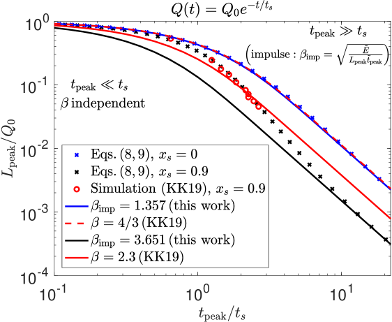
Following Khatami & Kasen (2019), we consider depositions that have a constant spatial distribution and a magnitude that is decreasing over time with a typical decay time of $t_{s}$ (specifically, $Q(t)=Q_{0}e^{-t/t_{s}}$). The luminosity can therefore be expressed as:

$$L(\tilde{t})=\int_{0}^{\tilde{t}}d\tilde{t}^{\prime}Q(\tilde{t}^{\prime})L_{\delta}(\tilde{t}-\tilde{t}^{\prime})$$ (8)

where $L_{\delta}(\tilde{t})$ is the luminosity obtained in the impulse approximation, $Q_{\delta}=\delta(\tilde{t})$, for the same spatial distribution of the deposition.

It is useful to consider Eq. (7) in two extremes. First, for a deposition time $t_{s}$ which is much longer than the diffusion time $t_{d}$, $\tilde{Q}$ is approximately constant beyond $t_{\rm peak}$ and equal to $\tilde{L}_{\rm peak}$. To see this, note that for constant deposition, $\tilde{L}$ is a monotonically increasing function (accumulation of $L_{\delta}$, Eq (8)) that is approximately equal to $\tilde{Q}$ at times much longer than the diffusion time. In this case, Eq. (7) is correct for any value of $\beta$ of order unity. Second, for a deposition time which is much shorter than the diffusion time (the impulse limit), the integral on the rhs of Eq. (7) reduces to the total deposition energy $\tilde{E}$, which is independent of $\beta$ and the specific source function. Therefore, Eq. (7) becomes correct for the choice $\beta_{\rm{imp}}=(\tilde{E}/(L_{\rm peak}\tilde{t}_{\rm peak}))^{1/2}$. These arguments imply that Eq. (7) (and thus Eq. (1)) is correct for $\beta=\beta_{\rm{imp}}$ for both very short $t_{s}\ll t_{d}$ and very long $t_{s}\gg t_{d}$ deposition times. Khatami & Kasen (2019) argued that for the special case of a uniform ejecta (uniform density and opacity), a single value of $\beta$ applies to a good approximation also for intermediate values of $t_{s}\sim t_{d}$. We show below that while this is true for central deposition, this is not the case for the extended depositions considered by Khatami & Kasen (2019).

The luminosity $L_{\delta}$ as a function of time $\tilde{t}$ from an impulse of energy $\tilde{E}=1$, deposited uniformly over $x_{s}$ within a ball of radius $R=1$, and diffusion coefficient $D=1$, is straight forward to derive and is given by

$$L_{\delta}=\frac{6}{x_{s}^{3}}\sum_{n=1}^{\infty}(-1)^{n+1}\left(\frac{\sin(n\pi x_{s})}{n\pi}-x_{s}\cos(n\pi x_{s})\right)e^{-n^{2}\pi^{2}\tilde{t}}.$$ (9)

For deposition radii of $x_{s}=0,0.33,0.9$ the peak times are $\tilde{t}_{peak}=0.09175,0.08012,0.004500$, the maximum luminosities are $L_{\rm peak}=5.922,5.963,16.67$ and the values of $\beta_{\rm{imp}}=1/(L_{\rm peak}\tilde{t}_{peak})^{1/2}$ are $1.357,1.447,3.651$, respectively. While the first two values are similar to the value $\beta=4/3$ reported by Khatami & Kasen (2019) for small $x_{s}$, the last value is significantly different from the value of $\beta=2.3$ that they report for the corresponding $x_{s}=0.9$. The source of the difference can be seen in figure 1,where the resulting peak luminosities are shown. For $x_{s}=0$, a single value $\beta=\beta_{\rm{imp}}\approx 4/3$ is a good approximation at all values of $t_{s}$, while for $x_{s}=0.9$, the value of $\beta=\beta_{\rm{imp}}=3.651$ fails in the intermediate regime of $t_{s}\sim t_{\rm peak}$. The value $\beta=2.3$, which Khatami & Kasen (2019) calibrated to the intermediate regime, does better but fails for very fast deposition.

A matlab function that calculates the luminosity as a function of time for a given mass, outer velocity, opacity, $x_{s}$, and $t_{s}$ using Eqs. (8),(9), is provided in this link.

Figure 1: Peak times and luminosities for the ejecta discussed in the text. The analytical results (equations Eqs. (8-9), blue crosses, $x_{s}=0$ and black crosses, $x_{s}=0.9$) agree and extend the results of the simulations of Khatami & Kasen (2019) (their figure 8, red dots, shown only for $x_{s}=0.9$). Solid lines are the analytic solutions of Eq. (1), for an exponential deposition (Khatami & Kasen, 2019) with corresponding values of $\beta$ as given in the legend. The data behind the figure is provided in this link.

References

• Arnett (1982) Arnett, W.Β D.Β 1982, ApJ, 253, 785
• Katz et al. (2013) Katz, B., Kushnir, D., & Dong, S.Β 2013, arXiv e-prints, arXiv:1301.6766
• Khatami & Kasen (2019) Khatami D.Β K., Kasen D.Β N., 2019, ApJ, 878, 56
• Pinto & Eastman (2000) Pinto, P.Β A., & Eastman, R.Β G.Β 2000, ApJ, 530, 744