Cross-correlation of the thermal Sunyaev–Zel’dovich effect and weak gravitational lensing: Planck and Subaru Hyper Suprime-Cam first-year data

Abstract

Cross-correlation analysis of the thermal Sunyaev–Zel’dovich (tSZ) effect and weak gravitational lensing (WL) provides a powerful probe of cosmology and astrophysics of the intra-cluster medium. We present the measurement of the cross-correlation of tSZ and WL from Planck and Subaru Hyper-Suprime Cam. The combination enables us to study cluster astrophysics at high redshift. We use the tSZ-WL cross-correlation and the tSZ auto-power spectrum measurements to place a tight constraint on the hydrostatic mass bias, which is a measure of the degree of non-thermal pressure support in galaxy clusters. With the prior on cosmological parameters derived from the analysis of the cosmic microwave background anisotropies by Planck and taking into account foreground contributions both in the tSZ auto-power spectrum and the tSZ-WL cross-correlation, the hydrostatic mass bias is estimated to be $26.9^{+8.9}_{-4.4}\%$ ($68\%$ C.L.), which is consistent with recent measurements by mass calibration techniques.

1 Introduction

The anisotropies of the cosmic microwave background (CMB) contain rich information on the energy content and evolution of our Universe. The so-called secondary CMB anisotropies, that are generated after last scattering, convey further information of the large-scale structures of the Universe. The Sunyaev–Zel’dovich (SZ) effect (Sunyaev & Zel’dovich, 1972, 1980) is the most important source of the secondary anisotropies, and it has been emerging as a powerful observational probe into the large-scale structure.

The thermal Sunyaev–Zel’dovich (tSZ) effect is caused by hot electrons contained in galaxy clusters, and it has been used to study the thermodynamic properties of the intra-cluster medium (ICM). Recently, Planck has detected the tSZ effect to a number of galaxy cluster with a high significance level (Planck Collaboration et al., 2016b), and several ground-based CMB experiments such as Atacama Cosmology Telescope (ACT, Swetz et al., 2011) and South Pole Telescope (SPT, Bleem et al., 2012) measured the tSZ effect with higher angular resolution.

Several analytical prescriptions have been proposed to model theoretically the tSZ effect and the evolution of ICM (e.g., Makino et al., 1998; Komatsu & Seljak, 2001; Bode et al., 2009; Shaw et al., 2010; Flender et al., 2017). The complexities of highly non-linear ICM physics make it challenging for such models to provide accurate theoretical predictions. Cosmological hydrodynamical simulations are often employed to investigate the formation and the evolution of the hot ICM (e.g., Nagai, 2006; Battaglia et al., 2012a, b; McCarthy et al., 2014; Dolag et al., 2016). Unfortunately, hydrodynamical simulations are computationally expensive, and there still remain statistical uncertainties owing to the limited simulation volume or to the small number of samples. In order to circumvent these problems, more observation-based approaches are proposed. Hydrodynamics simulations and self-similar models suggest that thermodynamic quantities such as temperature and pressure have universal profiles (Nagai et al., 2007b). Such a profile can be expressed by a fixed functional form with some free parameters, which are directly calibrated through X-ray and tSZ observations (Arnaud et al., 2010; Planck Collaboration et al., 2013). Note that the calibration can be performed for massive and nearby clusters, but often, mostly for simplicity, a universal pressure profile model is adopted in cosmological analysis of the tSZ effect. One of the critical assumptions usually made is hydrostatic equilibrium (HSE); the ICM is in dynamical equilibrium supported solely by the thermal pressure. With the HSE assumption, we can derive the mass of galaxy clusters from X-ray or tSZ observations in a simple manner, and can perform a variety of cosmological analyses.

Recent cosmological simulations show that galaxy clusters at high redshifts are not in a dynamically equilibrium state, and are often supported by the so-called non-thermal pressure (e.g., Nelson et al., 2014b; Shi et al., 2015; Vazza et al., 2018), in addition to the thermal pressure of ICM. Non-thermal pressure in the outer part of galaxy clusters has not yet been observed directly, and thus the cluster mass estimates based on the HSE assumption remain uncertain or inaccurate (e.g., Nagai et al., 2007a; Lau et al., 2009, 2013; Suto et al., 2013; Nelson et al., 2014a; Shi et al., 2016; Biffi et al., 2016; Henson et al., 2017). It is important to understand the origin and the contribution of non-thermal pressure in the next decade when large cosmological surveys are conducted; inaccurate cluster masses may lead to biased inference of cosmological parameters (Pratt et al., 2019, for a recent review).

The auto-power spectrum of the tSZ effect is widely used as a summary statistic for cosmological analyses. It is known that the amplitude of the tSZ power spectrum is very sensitive to the amplitude of the matter fluctuation, i.e., $\sigma_{8}$ (Komatsu & Seljak, 2002). At the angular-scales accessible by current observations, most of the cosmological information from the power spectrum is in its amplitude, and cosmological parameter inference suffers from the well-known degeneracy between parameters, e.g., matter density and $\sigma_{8}$ (Bolliet et al., 2018). A promising way to overcome this problem is cross-correlating the tSZ effect with another observable which traces the large-scale structure. Since the tSZ effect traces the large-scale structure through the pressure field in the Universe, it is expected that the cross-correlation can be detected at high significance level. In this work, we focus on the cross-correlation between the tSZ effect and weak gravitational lensing (WL), which is referred to as small distortion of images of background galaxies due to the gravitational potential generated by large-scale structure. The advantage of WL is that it can probe the line-of-sight integral of density contrast directly. We do not need to introduce uncertain galaxy bias. Various imaging surveys have successfully detected WL with high signal-to-noise ratio in sufficiently wide areas for cosmological studies (Kuijken et al., 2015; Zuntz et al., 2018).

The cross-correlation of tSZ and WL has already been detected (Van Waerbeke et al., 2014; Hojjati et al., 2017) and utilised to probe into the diffuse gas distribution (Ma et al., 2015). Osato et al. (2018) use the cross-correlation to constrain both cosmological parameters and the fractional contribution from non-thermal pressure. However, the capabilities of the measurements so far are limited due to low surface number density of source galaxies detected by shallow observations. In the present paper, we use the WL measurements by Subaru Hyper-Suprime Cam (Miyazaki et al., 2018; Aihara et al., 2018a; Mandelbaum et al., 2018a). The high image quality and the large aperture enable us to detect faint galaxies at high redshift. We can extract the information of the large-scale structure and ICM physics at high redshift that is not accessible by other WL surveys.

The rest of the paper is organized as follows. In Section 2, we describe the method to predict the auto-power spectrum of tSZ and the cross-correlation of tSZ and WL. Then, we describe WL survey by Hyper Suprime-Cam in Section 3, and tSZ observation by Planck in Section 4. In Section 5, details of mock simulations used for estimation of covariance matrix are described. We present the measurement of the cross-correlation in Section 6 and the cosmological analyses in Section 7. In Section 8, discussions on the results are presented and the concluding remarks are made in Section 9.

2 Formulation

In this Section, we present our analytic model to generate theoretical templates of the tSZ auto-power spectrum and the tSZ-WL cross-correlation.

2.1 The thermal Sunyaev–Zel’dovich effect

Here, we briefly review the basics of the tSZ effect. The temperature variation due to the tSZ effect is proportional to the line-of-sight integral of the electron pressure with respect to the physical distance $l$,

$$\frac{\Delta T}{T_{0}}=g_{\nu}(x)y=g_{\nu}(x)\frac{\sigma_{\mathrm{T}}}{m_{\mathrm{e}}c^{2}}\int\!\!P_{\mathrm{e}}\,dl,$$ (1)

where $T_{0}=2.725\,\mathrm{K}$ is the temperature of CMB photons, $y$ is the Compton-$y$ parameter, $\sigma_{\mathrm{T}}$ is the Thomson scattering cross-section, $m_{\mathrm{e}}$ is the electron mass, $c$ is the speed of light, and $P_{\mathrm{e}}$ is the electron pressure. The function $g_{\nu}(x)$ determines the dependence of the frequency $\nu$:

$$g_{\nu}(x)=x\frac{e^{x}-1}{e^{x}+1}-4,\ x=\frac{h\nu}{k_{\mathrm{B}}T_{0}},$$ (2)

where $h$ is the Planck constant and $k_{\mathrm{B}}$ is the Boltzmann constant. For very hot or relativistic electrons, relativistic corrections may become important (Itoh et al., 1998; Nozawa et al., 1998; Chluba et al., 2012) but we do not consider the typically small corrections in the following cosmological analysis.

2.2 Power spectrum of the tSZ effect

Since the Compton-$y$ is the integration of the product of density and temperature, the main contribution of tSZ comes from hot gas of clusters and the contribution from diffuse gas in the cluster outskirts and in filaments is subdominant. In order to model the power spectrum of Compton-$y$, we employ the so-called halo model, where all matter is associated with halos (Makino & Suto, 1993; Komatsu & Kitayama, 1999; Shaw et al., 2010).

The power spectrum can be decomposed into contributions from a single halo and clustered two halos, which are referred to as one-halo and two-halo terms, respectively. Then, the auto-power spectrum $C^{yy}(\ell)$ of the Compton-$y$ parameter is given as

$$C^{yy}(\ell)=C^{yy}_{\mathrm{1h}}(\ell)+C^{yy}_{\mathrm{2h}}(\ell).$$ (3)

The one-halo term is expressed as

$$C^{yy}_{\mathrm{1h}}(\ell)=\int\!\!dz\frac{d^{2}V}{dzd\Omega}\int\!\!dM\frac{dn(M,z)}{dM}|\tilde{y}_{\ell}(M,z)|^{2},$$ (4)

where $d^{2}V/dzd\Omega=D_{A}^{2}(z)(c/H(z))$ is the comoving volume per redshift and solid angle, $D_{A}(z)$ is the comoving angular diameter distance, and $dn(M,z)/dM$ is the halo mass function. The 2D Fourier transform of the Compton-$y$ parameter $\tilde{y}_{\ell}(M,z)$ is given as

$$\tilde{y}_{\ell}(M,z)=\frac{4\pi r_{s}}{\ell_{s}^{2}}\left(\frac{\sigma_{\mathrm{T}}}{m_{e}c^{2}}\right)\int\!\!dx\,x^{2}P_{\mathrm{e}}(x;M,z)\frac{\sin(\ell x/\ell_{s})}{\ell x/\ell_{s}},$$ (5)

where $r_{s}$ is the arbitrary scale radius, $\ell_{s}=(1+z)^{-1}D_{A}(z)/r_{s}$, and $P_{\mathrm{e}}(x;M,z)$ is the electron pressure profile with respect to the scaled radius $x\equiv r/r_{s}$. We define the halo radius $R_{\Delta}$ as the radius within which the mean density is equal to $\Delta$ times the critical density $\rho_{\mathrm{cr}}(z)$. Then, the enclosed mass $M_{\Delta}$ is given as

$$M_{\Delta}=\frac{4\pi}{3}\Delta\rho_{\mathrm{cr}}(z)R_{\Delta}^{3}.$$ (6)

We adopt the virial halo mass $M_{\mathrm{vir}}$, which overdensity $\Delta_{\mathrm{vir}}$ is computed from spherical collapse model (Bryan & Norman, 1998),

$$\Delta_{\mathrm{vir}}=18\pi^{2}+82(\Omega_{\mathrm{m}}(z)-1)-39(\Omega_{\mathrm{m}}(z)-1)^{2},$$ (7)

where $\Omega_{\mathrm{m}}(z)$ is the matter density normalized by the critical density at redshift $z$:

$$\Omega_{\mathrm{m}}(z)=\Omega_{\mathrm{m}}(1+z)^{3}E^{-2}(z),$$ (8)

and $E(z)$ is the expansion factor:

$$E(z)=\frac{H(z)}{H_{0}}=[\Omega_{\mathrm{m}}(1+z)^{3}+1-\Omega_{\mathrm{m}}]^{\frac{1}{2}}.$$ (9)

Here, $\Omega_{\mathrm{m}}$ is the present value of matter density normalized by the critical density and we assume the flat $\Lambda$ cold dark matter (CDM) Universe. There are alternative halo mass definitions. One is the critical overdensity masses, $M_{200}$ and $M_{500}$, which mean density is equal to $200$ and $500$ times the critical density $\rho_{\mathrm{cr}}(z)$, respectively. Furthermore, we also adopt the mean overdensity mass $M_{\mathrm{200m}}$, which mean density is equal to $200$ times the background matter density $\rho_{\mathrm{m}}(z)$. Note that all masses can be converted interchangeably once the mass and the concentration parameter (see Section 2.3) are specified for one mass definition. Throughout halo model calculations, we use $M_{\mathrm{vir}}$ as the definition of the halo mass $M$.

Next, the two-halo term is given by

$$C^{yy}_{\mathrm{2h}}(\ell) = \int\!\!dz\frac{d^{2}V}{dzd\Omega}P_{\mathrm{m}}\left(k=\frac{\ell+1/2}{D_{A}(z)},z\right)$$ (10)

$$\times\left[\int\!\!dM\frac{dn(M,z)}{dM}\tilde{y}_{\ell}(M,z)b_{\mathrm{h}}(M,z)\right]^{2},$$

where $b_{\mathrm{h}}(M,z)$ is the halo bias and $P_{\mathrm{m}}(k,z)$ is the 3D linear matter power spectrum. Finally, we can compute the power spectrum of Compton-$y$, if the halo mass function, halo bias, cosmological parameters, and pressure profile are specified. We adopt the fitting formulas of halo mass function of Bocquet et al. (2016) and halo bias of Tinker et al. (2010), where the mean overdensity mass $M_{\mathrm{200m}}$ is adopted as the halo mass definition. We use the linear Boltzmann code CAMB (Lewis et al., 2000) to compute the linear matter power spectrum.

In computing the Fourier transform of the Compton-$y$ parameter $\tilde{y}_{\ell}(M,z)$, we adopt the universal pressure profile of Nagai et al. (2007b). The explicit form is given by

$$\frac{P_{\mathrm{e}}(r)}{P_{500}} = p(x)\left[\frac{M^{\mathrm{HSE}}_{\mathrm{500}}}{3\times 10^{14}h_{70}^{-1}\mathrm{M}_{\sun}}\right]^{0.12},$$ (11)

$$p(x) \equiv \frac{P_{0}}{(c_{500}x)^{\gamma}[1+(c_{\mathrm{500}}x)^{\alpha}]^{(\beta-\gamma)/\alpha}},$$ (12)

$$P_{500} = 1.65\times 10^{-3}E(z)^{8/3}$$ (13)

$$\times\left[\frac{M^{\mathrm{HSE}}_{\mathrm{500}}}{3\times 10^{14}h_{70}^{-1}\mathrm{M}_{\sun}}\right]^{2/3}h_{70}^{2}\,\mathrm{keV}\,\mathrm{cm}^{-3},$$

where $x=r/R^{\mathrm{HSE}}_{500}$ and $h_{70}=h/0.7$. This formula contains several free parameters, which are directly fitted to data from X-ray or SZ observations of the cluster pressure profile. With the measurements of SZ selected clusters (Planck Collaboration et al., 2013), the parameters are calibrated as

$$(P_{0},c_{500},\gamma,\alpha,\beta)=(6.41,1.81,0.31,1.33,4.13).$$ (14)

Note that the cluster mass is estimated with HSE assumption and thus is likely underestimated compared with the true mass. In order to relate the HSE mass with true mass, we introduce the hydrostatic bias parameter $b_{\mathrm{HSE}}$ and scale the mass and radius as $M^{\mathrm{HSE}}_{\mathrm{500}}=M_{\mathrm{500}}(1-b_{\mathrm{HSE}})$ and $R^{\mathrm{HSE}}_{500}=R_{500}(1-b_{\mathrm{HSE}})^{1/3}$. Typically, $b_{\mathrm{HSE}}=0.15\text{--}0.40$ is estimated from WL mass calibration measurements and also from hydrodynamical simulations (see Sections 8.2 and 8.3 for more details and references therein).

2.3 Cross-correlations of tSZ and WL

Similarly to the auto-power spectrum, the cross-power spectrum of Compton-$y$ and convergence field is also computed based on halo model:

$$C^{y\kappa}(\ell) = C^{y\kappa}_{\mathrm{1h}}(\ell)+C^{y\kappa}_{\mathrm{2h}}(\ell),$$ (15)

$$C^{y\kappa}_{\mathrm{1h}}(\ell) = \int\!\!dz\frac{d^{2}V}{dzd\Omega}\int\!\!dM\frac{dn(M,z)}{dM}\tilde{y}_{\ell}(M,z)\tilde{\kappa}_{\ell}(M,z),$$ (16)

$$C^{y\kappa}_{\mathrm{2h}}(\ell) = \int\!\!dz\frac{d^{2}V}{dzd\Omega}P_{\mathrm{m}}\left(k=\frac{\ell+1/2}{D_{A}(z)},z\right)$$ (17)

$$\times\int\!\!dM\frac{dn(M,z)}{dM}\tilde{y}_{\ell}(M,z)b_{\mathrm{h}}(M,z)$$

$$\times\int\!\!dM\frac{dn(M,z)}{dM}\tilde{\kappa}_{\ell}(M,z)b_{\mathrm{h}}(M,z).$$

Compared with the formulas of the auto-power spectrum (Eqs. 3, 4, and 10), one of the Fourier transform of Compton-$y$ $\tilde{y}_{\ell}(M,z)$ is replaced with the Fourier transform of the convergence from a single halo $\tilde{\kappa}_{\ell}(M,z)$. Before moving onto the explicit expression of $\tilde{\kappa}_{\ell}(M,z)$, we review the basics of the halo density profile, which is critical to model the lensing signal. It is assumed that the density profile has a spherical profile, so-called Navarro–Frenk–White (NFW) profile (Navarro et al., 1996, 1997):

$$\rho(r)=\frac{\rho_{s}}{(r/r_{s})(1+r/r_{s})^{2}},$$ (18)

where $\rho_{s}$ is the scale density and $r_{s}$ is the scale radius. Since this density profile scales as $\propto r^{-3}$ at large radii, the enclosed mass does not converge. Thus, we truncate the profile at the virial radius $R_{\mathrm{vir}}$ determined through Eqs. (6) and (7). Then, the virial halo mass is given as

$$M_{\mathrm{vir}}=\int_{0}^{R_{\mathrm{vir}}}\!\!\rho(r)4\pi r^{2}dr=4\pi\rho_{s}r_{s}^{3}m_{\mathrm{NFW}}(c),$$ (19)

where

$$m_{\mathrm{NFW}}(c)=\int_{0}^{c}\frac{r}{(1+r)^{2}}\,dr=\ln(1+c)-\frac{c}{1+c},$$ (20)

and $c=R_{\mathrm{vir}}/r_{s}$ is the concentration parameter. In order to determine the profile, we need to specify the scale radius $r_{s}$ and the scale density $\rho_{s}$. It is known that the scale radius is correlated with the halo mass, and the fitting formula of the concentration parameter as a function of virial mass and redshift is used. Throughout this paper, we adopt the fitting formula in Klypin et al. (2016) calibrated with $N$-body simulations. As a result, for a given virial mass, the density profile is uniquely determined. Then, the Fourier transform of the scaled density profile $u(r)=\rho(r)/M$ is given as

$$\tilde{u}_{M}(k) \equiv \int d^{3}r\,u(r)e^{-i\bm{k}\cdot\bm{r}}$$ (22)

$$= \frac{1}{m_{\mathrm{NFW}}(c)}\left[\sin x\{\mathrm{Si}[x(1+c)]-\mathrm{Si}(x)\}\right.$$

$$+\cos x\{\mathrm{Ci}[x(1+c)]-\mathrm{Ci}(x)\}$$

$$\left.-\frac{\sin(xc)}{x(1+c)}\right],$$

where $x\equiv(1+z)kr_{s}$, $\mathrm{Si}(x)$ and $\mathrm{Ci}(x)$ are sine and cosine integrals, respectively (Scoccimarro et al., 2001). The Fourier transform of the convergence profile $\kappa(\theta)$ from a single halo with mass $M$ is given by

$$\tilde{\kappa}_{\ell}(M,z)=\int 2\pi\theta\kappa(\theta)J_{0}(\ell\theta)\,d\theta=\frac{M\tilde{u}_{M}(k=\ell/D_{A}(z),z)}{D_{A}^{2}(z)\Sigma_{\mathrm{cr}}(z)},$$ (23)

where $J_{0}(x)$ is the zeroth order Bessel function. The critical surface mass density $\Sigma_{\mathrm{cr}}(z)$ is given as

$$\Sigma_{\mathrm{cr}}^{-1}(z)=\frac{4\pi G}{c^{2}}\chi(z)(1+z)^{-1}\left[1-\chi(z)\left\langle\frac{1}{\chi(z_{s})}\right\rangle\right],$$ (24)

where $\chi(z)$ is the comoving distance and

$$\left\langle\frac{1}{\chi(z_{s})}\right\rangle=\left[\int dz_{s}\frac{dp}{dz_{s}}\frac{1}{\chi(z_{s})}\right]\left[\int dz_{s}\frac{dp}{dz_{s}}\right]^{-1}.$$ (25)

The stacked probability distribution function (PDF) of source galaxy redshifts $p(z)$ needs to be given by the actual catalog and only the stacked PDF depends on the observational data in this prescription. By summing up PDFs of all source galaxies, dilution effect is mitigated though it is not completely removed (see also Medezinski et al., 2018). In the subsequent analysis, we adopt Ephor AB with reweights derived from COSMOS 30 band observations as our fiducial choice (see Section 3.3).

2.4 Differential contribution with respect to halo mass and redshift

In the halo model, the tSZ auto-power spectrum and tSZ-WL cross-power spectrum have been sourced by halos with various ranges of mass and redshift. To investigate the mass and redshift ranges of which halos contribute to the spectra the most, we compute the differential contribution for both of spectra. From Eqs. (3), (4), and (10), the differential contribution for tSZ auto-power spectrum with respect to the halo mass and redshift is given by

$$\frac{d^{2}C^{yy}(\ell)}{dzdM} = \frac{d^{2}C^{yy}_{\mathrm{1h}}(\ell)}{dzdM}+\frac{d^{2}C^{yy}_{\mathrm{2h}}(\ell)}{dzdM},$$ (26)

$$\frac{d^{2}C^{yy}_{\mathrm{1h}}(\ell)}{dzdM} = \frac{d^{2}V}{dzd\Omega}\frac{dn(M,z)}{dM}|\tilde{y}_{\ell}(M,z)|^{2},$$ (27)

$$\frac{d^{2}C^{yy}_{\mathrm{2h}}(\ell)}{dzdM} = \frac{d^{2}V}{dzd\Omega}P_{\mathrm{m}}\left(k=\frac{\ell+1/2}{D_{A}(z)},z\right)$$ (28)

$$\times 2\left[\frac{dn(M,z)}{dM}\tilde{y}_{\ell}(M,z)b_{\mathrm{h}}(M,z)\right.$$

$$\left.\int\!\!dM\frac{dn(M,z)}{dM}\tilde{y}_{\ell}(M,z)b_{\mathrm{h}}(M,z)\right].$$

Similarly for the tSZ-WL cross-power spectrum, from Eqs. (15), (16), and (17), the differential contribution of the cross-power spectrum is given by

$$\frac{d^{2}C^{y\kappa}(\ell)}{dzdM} = \frac{d^{2}C^{y\kappa}_{\mathrm{1h}}(\ell)}{dzdM}+\frac{d^{2}C^{y\kappa}_{\mathrm{2h}}(\ell)}{dzdM},$$ (29)

$$\frac{d^{2}C^{y\kappa}_{\mathrm{1h}}(\ell)}{dzdM} = \frac{d^{2}V}{dzd\Omega}\frac{dn(M,z)}{dM}\tilde{y}_{\ell}(M,z)\tilde{\kappa}_{\ell}(M,z),$$ (30)

$$\frac{d^{2}C^{y\kappa}_{\mathrm{2h}}(\ell)}{dzdM} = \frac{d^{2}V}{dzd\Omega}P_{\mathrm{m}}\left(k=\frac{\ell+1/2}{D_{A}(z)},z\right)$$ (31)

$$\times\left[\frac{dn(M,z)}{dM}\tilde{y}_{\ell}(M,z)b_{\mathrm{h}}(M,z)\right.$$

$$\times\int\!\!dM\frac{dn(M,z)}{dM}\tilde{\kappa}_{\ell}(M,z)b_{\mathrm{h}}(M,z)$$

$$+\frac{dn(M,z)}{dM}\tilde{\kappa}_{\ell}(M,z)b_{\mathrm{h}}(M,z)$$

$$\times\left.\int\!\!dM\frac{dn(M,z)}{dM}\tilde{y}_{\ell}(M,z)b_{\mathrm{h}}(M,z)\right].$$

In Figure 1, the differential contributions for three multipoles $\ell=10,100,1000$ are shown. Though both of spectra are sensitive to the similar range of halo mass and redshift for $\ell=1000$, for other multipoles, less massive and higher redshift halos contribute to the tSZ-WL cross-power spectrum. This result clearly shows the tSZ auto-power spectrum and tSZ-WL cross-power spectrum contain the information from different classes of halos.

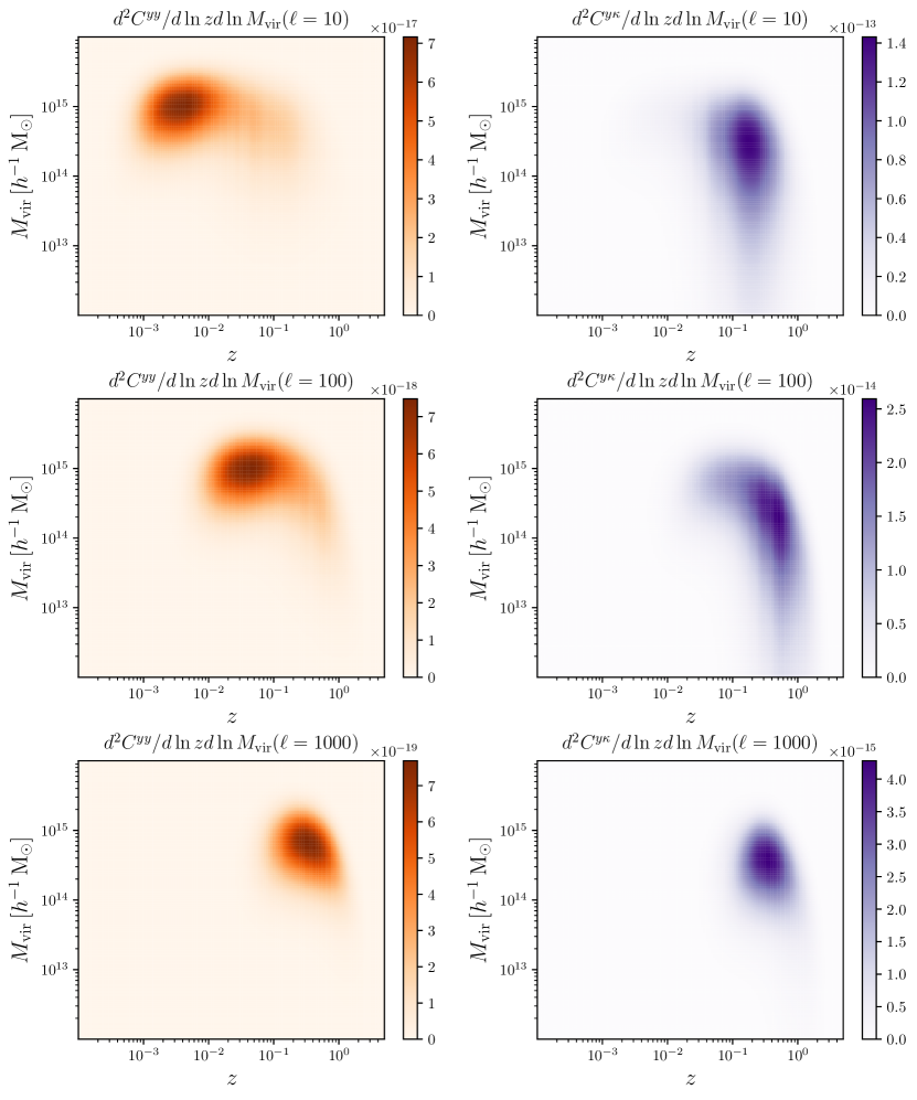
Figure 1: Differential contributions with respect to halo mass and redshift for tSZ auto-power spectrum (left panels) and tSZ-WL cross-power spectrum (right panels). In each row, the contributions for multipoles $\ell=10,100,1000$ are shown. Note that the plotted differential contributions are with respect to $\ln z$ and $\ln M_{\mathrm{vir}}$, instead of $z$ and $M_{\mathrm{vir}}$.

3 Weak lensing analysis with HSC S16A

3.1 Shape catalog

Subaru Hyper Suprime-Cam (HSC) is the imaging camera (Miyazaki et al., 2015, 2018) mounted on the prime focus of the Subaru telescope. HSC has the excellent wide field of view of $1.5\,\mathrm{deg}$ diameter, which corresponds to $1.77\,\mathrm{deg}^{2}$. The HSC survey (Aihara et al., 2018a, b) is composed of three layers according to science targets and depth: Wide, Deep, and UltraDeep. The WL analysis makes use of Wide layer data, which will cover $1400\,\mathrm{deg}^{2}$ over six years for five broad-bands, $grizy$.

The first-year HSC shape catalog, labelled as S16A, is based on observation data taken from 2014 March to 2016 April for about 90 nights. We employ cuts to the whole galaxy sample to create the shape catalog. Such cuts include a cmodel magnitude cut $i<24.5$ (for definitions of cmodel magnitude in the HSC survey, see Bosch et al., 2018), in contrast to the magnitude limit of HSC ($i\sim 26.4$). In addition, galaxies which point spread function (PSF) is failed to be estimated are removed and the regions affected by bright stars are masked. Thus, the shape catalog is constructed in a conservative manner. For each galaxy which passes all the criteria, we estimate the ellipticity $\bm{e}$ with the re-Gaussianization PSF correction method (Hirata & Seljak, 2003) for $i$-band co-added images:

$$\bm{e}=(e_{1},e_{2})=\frac{1-(b/a)^{2}}{1+(b/a)^{2}}(\cos 2\phi,\sin 2\phi),$$ (32)

where $b/a$ is the minor-to-major axis ratio of galaxy images and $\phi$ is the polar argument of the major axis. The resultant shape catalog is defined for $136.9\,\mathrm{deg}^{2}$ and the survey region is split into six patches: GAMA15H, WIDE12H, GAMA09H, VVDS, XMM, and HECTOMAP.

Here we describe additional quantities in the shape catalog used for our analysis. The full production process of the shape catalog and associated image simulations are outlined in Mandelbaum et al. (2018a) and Mandelbaum et al. (2018b), respectively. The S16A shape catalog has the per-component rms galaxy shape of a galaxy population $e_{\mathrm{rms}}$ for each source galaxy which is calibrated against the image simulations, and the weight $w_{i}$ which is defined as the inverse-variance weight with $e_{\mathrm{rms}}$ and the measurement noise caused by photon noise. The S16A galaxy shapes should be calibrated using the multiplicative bias factor $m$ and additive bias $c_{\alpha}$, where $m$ is shared among the ellipticity components and $c_{\alpha}$ is defined for an ellipticity component $\alpha$. These calibration factors are derived from the image simulations.

3.2 Reconstruction of the convergence field

In order to derive the weak lensing convergence field, we employ Kaiser–Squires inversion (hereafter, KS inversion) method (Kaiser & Squires, 1993). We follow the analysis of Oguri et al. (2018), where the same shape catalog is used. First, we estimate the shear filed from the shape of source galaxies

$$\hat{\gamma}_{\alpha}(\bm{\theta})=\frac{\sum_{i}w_{i}(\gamma_{\alpha}(\bm{\theta}_{i})-c_{\alpha,i})W_{\mathrm{G}}(|\bm{\theta}-\bm{\theta}_{i}|)}{\sum_{i}w_{i}(1+m_{i})W_{\mathrm{G}}(|\bm{\theta}-\bm{\theta}_{i}|)},$$ (33)

where $w_{i}$ is the lens weight, $\gamma_{\alpha}(\bm{\theta}_{i})$ is the local shear estimated as $\gamma_{\alpha}(\bm{\theta}_{i})=e_{\alpha,i}/2\mathcal{R}$ with the galaxy shape ellipticity $e_{\alpha,i}$ and the shear responsivity $\mathcal{R}$. Hereafter, the subscript $i$ runs over all source galaxies in the patch. The shear responsivity $\mathcal{R}$ is evaluated as

$$\mathcal{R}=1-\frac{\sum_{i}w_{i}e_{\mathrm{rms},i}^{2}}{\sum_{i}w_{i}},$$ (34)

where $e_{\mathrm{rms},i}$ is the intrinsic shape dispersion. The shear responsivity is evaluated for each patch. We apply smoothing with the Gaussian kernel $W_{\mathrm{G}}(\theta)$:

$$W_{\mathrm{G}}(\theta)=\frac{1}{\pi\theta_{s}^{2}}\exp\left(-\frac{\theta^{2}}{\theta_{s}^{2}}\right),$$ (35)

where the smoothing scale $\theta_{s}$ is adopted as $\theta_{s}^{\kappa}=2\,\mathrm{arcmin}$. This choice of the smoothing kernel ensures maps with high signal-to-noise ratio (Oguri et al., 2018). The additive and multiplicative biases, $c_{\alpha,i}$ and $m_{i}$, are calibrated with image simulations in Mandelbaum et al. (2018b). Then, we convert the shear field to the convergence field as

$$\hat{\kappa}(\bm{\theta})=\frac{1}{\pi}\int d^{2}\theta^{\prime}\frac{\gamma_{\mathrm{t}}(\bm{\theta}|\bm{\theta}^{\prime})}{|\bm{\theta}-\bm{\theta}^{\prime}|^{2}},$$ (36)

where $\gamma_{\mathrm{t}}(\bm{\theta}|\bm{\theta}^{\prime})$ is the tangential shear at the position $\bm{\theta}$ with respect to $\bm{\theta}^{\prime}$.

In the practical analysis, we adopt the flat-sky approximation. First, we compute the pixelized shear field on the regular grid with the pixel size of $0.5\,\mathrm{arcmin}$ for each patch of the survey regions, where the boundaries are determined by the positions of the source galaxies. Though the window function $W_{\mathrm{G}}(\bm{\theta})$ is always non-zero, we truncate it so that the function is forced to be zero outside the square with a side length $8\theta_{s}^{\kappa}$ centered on each galaxy position. Then, we apply fast Fourier transform (FFT) to the shear field and from Eq. (36), the Fourier transform of convergence field is given as

$$\hat{\kappa}(\bm{\ell})=\frac{(\ell_{1}+i\ell_{2})^{2}}{\ell^{2}}\hat{\gamma}(\bm{\ell}).$$ (37)

Then, the convergence field is obtained by inverse FFT. Although the convergence field should be a real function, the resultant field may have imaginary components. The real and imaginary parts are called as $E$- and $B$-mode convergence, respectively. In the subsequent analysis, we use only $E$-mode convergence, which we simply refer to as the convergence field, and the $B$-mode will be used for null tests (see Section 6.2).

We also compute smoothed number density field:

$$n(\bm{\theta})=\sum_{i}W_{\mathrm{G}}(|\bm{\theta}-\bm{\theta}_{i}|).$$ (38)

In order to remove the effects due to boundary and low density pixels, we mask the pixel where the smoothed number density is less than the half of the mean number density. The total area after masking is $161.66\,\mathrm{deg}^{2}$. We summarize properties for each patch in Table 1 and show the reconstructed convergence field in Figure 2. Note that the area of survey regions defined in shape catalogs is $136.9\,\mathrm{deg}^{2}$ but the convergence map covers $161.66\,\mathrm{deg}^{2}$ because of the non-local nature of reconstruction.

Table 1: Number of source galaxies, area after masking, and mean smoothed number density for six survey patches and all survey regions.

Field	Number of galaxies	Area ($\mathrm{deg}^{2}$)	Mean smoothed number density ($\mathrm{deg}^{-2}$)
GAMA15H	$2794258$	$34.54$	$17.90$
WIDE12H	$1219607$	$14.31$	$18.05$
GAMA09H	$3005495$	$41.01$	$15.91$
VVDS	$1843091$	$22.25$	$17.22$
XMM	$2596006$	$32.47$	$17.29$
HECTOMAP	$1157693$	$17.09$	$12.75$
All fields	$12616150$	$161.66$	—

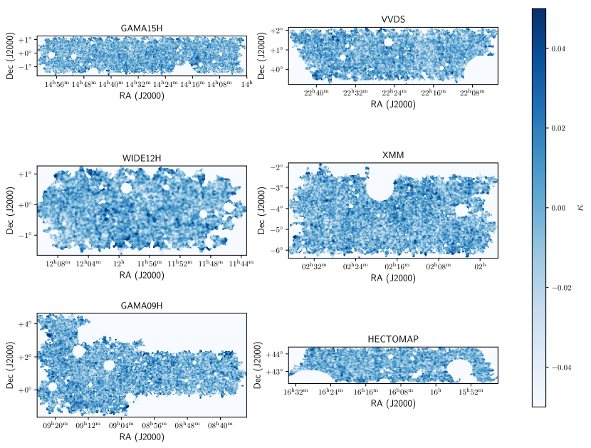
Figure 2: The reconstructed convergence fields with HSC S16A shape catalogs for six different survey patches: GAMA15H, WIDE12H, GAMA09H, VVDS, XMM, and HECTOMAP.

3.3 Source Redshift Distributions

To calculate the WL convergence, we need the stacked PDF of the source galaxy redshifts (see Section 2.3). We sum up PDFs of all galaxies in the S16A shape catalogs. There are a number of algorithms to estimate the photometric redshifts of source galaxies (for details, see Tanaka et al., 2018). Figure 3 shows the stacked PDFs of source galaxy redshifts derived using eight different algorithms. Since HSC can detect faint galaxies, the resultant PDF has a tail at high redshifts. As a fiducial model, we employ the stacked PDF estimated with Ephor AB code by reweighting the PDF obtained from the COSMOS 30-band observation catalog (Ilbert et al., 2009; Laigle et al., 2016) so that the distributions of magnitudes for five bands of HSC should match with that of galaxies used in the analysis (for details, see Section 5.2 of Hikage et al., 2019). We confirm that the different algorithms give consistent results within a few per-cent for calculations of cross-correlations (see Appendix A).

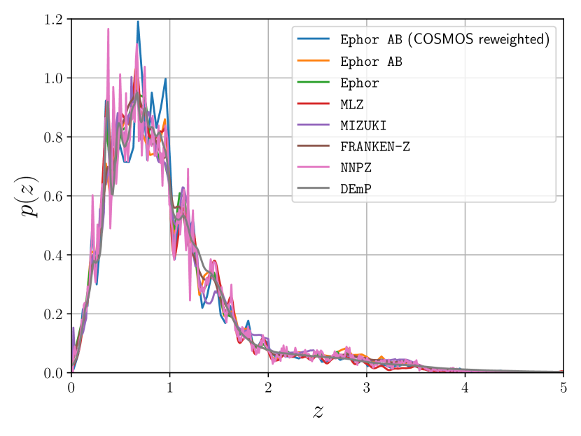
Figure 3: The stacked PDFs of source galaxy redshifts for different algorithms: Ephor AB with COSMOS reweight, Ephor AB, Ephor, MLZ, MIZUKI, FRANKEN-Z, NNPZ, and DEmP. Our fiducial choice is Ephor AB with COSMOS reweight.

3.4 Blinding

In the current situation where many cosmological results, e.g., constraints on cosmological parameters, are available, there is a risk that if the analysis becomes consistent with other results, the further analysis will not be carried out and the possible systematics will not be investigated any longer. This degrades the credibility and quality of the analysis, and is called as confirmation bias. In order to avoid the confirmation bias and derive robust results, we follow a blinding scheme in our analysis. In practice, we adopt two-tiers blinding of the multiplicative bias, i.e.,

$$\bm{m}^{\text{cat}}_{i}=\bm{m}^{\text{true}}+d\bm{m}^{(1)}_{i}+d\bm{m}^{(2)}_{i}\ (i=0,1,2),$$ (39)

where $\bm{m}^{\text{cat}}_{i}$ is the array of multiplicative bias stored in the shape catalog. The first term $d\bm{m}^{(1)}_{i}$ is added to avoid the case where the analysis lead accidentally finds true catalog when one of multiple projects is unblinded. This term is decrypted every time the catalog is used but not referenced directly. The second term $d\bm{m}^{(2)}_{i}$ is the factor disclosed by a blinder after all necessary analysis and unblinding procedure are performed. One of $d\bm{m}^{(2)}_{i}\ (i=0,1,2)$ is exactly zero, which corresponds to the true catalog, and the index of the true catalog is notified to the analysis lead from the blinder because only the blinder can decrypt $d\bm{m}^{(2)}_{i}$. Once the true catalog is disclosed, all of the results are fixed and further analysis and modification of the analysis pipeline are prohibited. The details of the blinding scheme are found in Section 3.2 of Hikage et al. (2019).

4 The thermal Sunyaev–Zel’dovich effect measured by Planck

Here, we briefly review the construction process of Compton-$y$ maps from Planck measurements. All of details are found in Planck Collaboration et al. (2016a). The Compton-$y$ map of Planck is constructed from $30$ to $857\,\mathrm{GHz}$ channel maps of the Planck full mission data with component separation algorithm. The map is pixelized in Healpix (Górski et al., 2005) format with $N_{\mathrm{side}}=2048$. The beam properties are different between the maps observed by different bands, but we assume circularly symmetric Gaussian beam with the full-width half-mean (FWHM) beam size $\theta_{\mathrm{FWHM}}=10.0\,\mathrm{arcmin}$ for the Compton-$y$ map, which corresponds to the Gaussian window scale $\theta_{s}^{y}=\theta_{\mathrm{FWHM}}/(2\sqrt{\log 2})=6.0\,\mathrm{arcmin}$ (see Eq. 35). The Planck team provides maps with two different component separation algorithm: MILCA (Modified Internal Linear Combination Algorithm, Hurier et al., 2013) and NILC (Needlet Independent Linear Combination, Remazeilles et al., 2011), both of which basically try to find the linear combination of several components so that the variance of the reconstructed map is minimized. Hereafter, we use the map constructed with MILCA as the fiducial map because it has lower noise contribution at large scales. When measuring the auto-power spectrum of Compton-$y$, the effect due to contamination originating from systematics must be minimized. To this end, the full mission data are separated by half, and the cross-power spectrum between the separated first and second maps is used as a baseline power spectrum. We make use of the full mission data for the measurement of the cross-correlations because such systematics do not correlate with the lensing convergence field. In addition, we mask galactic planes and point sources, where strong radio emission component separation becomes unreliable. We employ the 40% galactic mask and point source mask provided by Planck collaboration. We show the MILCA Compton-$y$ map together with HSC S16A survey patches in Figure 4.

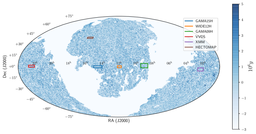
Figure 4: The Compton-$y$ map measured by Planck based on the MILCA algorithm. The six boxes indicate the HSC S16A survey patches. The 40% galactic mask and the point source mask have been applied.

5 Mock observations

In this Section, we present details of mock observations of tSZ and WL. We measure the tSZ auto-power spectrum and tSZ-WL cross-correlations from mock observations, and the results are used to estimate the covariance matrix. We also use these mock catalogues for null tests (Section 6.2) and evaluate the significance of our cross-correlation measurement (Section 6.3).

5.1 All-sky mock Compton-$y$ maps

We generate mock tSZ maps from all-sky halo catalogs of Takahashi et al. (2017). In the simulations, cosmological parameters are adopted from WMAP 9-year results (Hinshaw et al., 2013): the CDM density parameter $\Omega_{\mathrm{cdm}}=0.233$, the baryon density parameter $\Omega_{\mathrm{b}}=0.046$, the matter density parameter $\Omega_{\mathrm{m}}=\Omega_{\mathrm{cdm}}+\Omega_{\mathrm{b}}=0.279$, the cosmological constant density $\Omega_{\Lambda}=0.721$, the scaled Hubble constant $h=0.7$, the amplitude of the matter power spectrum $\sigma_{8}=0.82$, and the spectral index of the scalar perturbation $n_{\mathrm{s}}=0.97$. From the halo catalog, we construct the all-sky tSZ map by pasting the universal pressure profile with $b_{\mathrm{HSE}}=0.2$ onto each halo in the catalog. First, we create 108 mock tSZ maps from the halo catalog. Next, we smooth the tSZ map with the circular Gaussian window function with the Gaussian window scale $\theta^{y}_{s}=6.0\,\mathrm{arcmin}$. Finally, we apply the $40\%$ galactic and radio point source masks. The sky coverage fraction after masking is $f_{\mathrm{sky}}=0.512$. We do not add instrumental noise to the mock maps because the amplitude of the noise is uncertain and the foreground noise is dominant.

In order to remove the artificial mode coupling induced by masking, we deconvolve the mask spectrum from the pseudo-spectrum using MASTER algorithm (Hivon et al., 2002). The relation between the pseudo-power spectrum $\tilde{C}_{\ell}$, which is measured directly from mock maps, and the true power spectrum $C_{\ell}$ can be given as

$$\tilde{C}_{\ell}=\sum_{\ell^{\prime}}M_{\ell\ell^{\prime}}B^{2}_{\ell^{\prime}}C_{\ell^{\prime}},$$ (40)

where $M_{\ell\ell^{\prime}}$ is the mode-coupling matrix, and $B_{\ell}$ is the window function describing smoothing effects of the beam and finite pixelization of Healpix. The mode-coupling matrix is given as

$$M_{\ell_{1}\ell_{2}}=\frac{2\ell_{2}+1}{4\pi}\sum_{\ell_{3}}(2\ell_{3}+1)W_{\ell_{3}}\begin{pmatrix}\ell_{1}&\ell_{2}&\ell_{3}\\ 0&0&0\\ \end{pmatrix}^{2},$$ (41)

where $W_{\ell}$ is the mask power spectrum, and the last term is the Wigner-$3j$ symbol. Then, we invert Eq. (40) to obtain the true power spectrum $C_{\ell}$ from the pseudo-power spectrum $\tilde{C}_{\ell}$. Figure 5 shows auto-power spectra of Compton-$y$ from 108 mock all-sky Compton-$y$ maps. These mock measurements are used to estimate the covariance matrix of tSZ auto-power spectra. For a few realizations, the excessive signals can be seen. These correspond to the cases where massive clusters are located at low redshifts by chance.

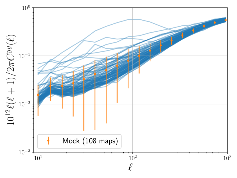
Figure 5: The power spectra measured from mock Compton-$y$ maps. Each blue solid line corresponds to one measurement with a mock map. The orange points with error bars show the mean and standard deviation among 108 mock maps. Note that the standard deviation is computed for the raw power spectrum, not logarithm of it. Thus, the lower limit of the error looks smaller than the distribution of power spectra. Another cause is that the distribution of power spectra at large scales are not well approximated as Gaussian distribution.

5.2 Mock shape catalog

In order to create mock convergence maps, we employ the mock shape catalog created in Shirasaki et al. (2019). The mock catalog is specifically designed for the HSC survey and constructed directly from the S16A shape catalog. The same all-sky simulations (Takahashi et al., 2017) in creating mock Compton-$y$ maps are employed. First, we randomly rotate the shapes of all galaxies in the catalog to remove the lensing signal. Then, we take the all-sky lensing map, and deform the shape again according to the shear and convergence at the position of each galaxy. The redshift of each galaxy is determined by random sampling from the PDF estimated with MLZ. Finally, we obtain realistic catalogs which contain the lensing signal and observational effects, e.g., discrete distribution of source galaxies and photometric redshift distribution. Moreover, other quantities derived in the shape measurement, e.g., lens weights, are also attached to the mock catalog and thus we can carry out mock measurements in almost the same way to the real measurements.

Figure 6 shows convergence maps and corresponding regions in the mock Compton-$y$ map. It is clearly seen that massive clusters yield the strong signals at the same positions in on both of the maps. We can extract 21 HSC regions from one realization of the all-sky map, and we compute the cross-correlation from these maps for a total of $108\times 21=2268$ realizations. Figure 7 shows cross-correlations obtained from our 2268 mock maps. The mock measurements are used to estimate the covariance matrix of the cross-correlation. Similarly to mock auto-power spectra, signals with very high amplitudes are observed in several mock measurements. This is also associated with massive clusters at low redshifts.

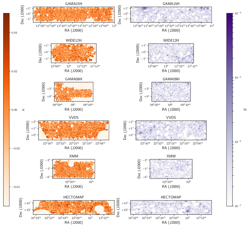
Figure 6: An example of a mock convergence map (left panels) and a mock Compton-$y$ map (right panels). The Compton-$y$ maps are extracted from the original all-sky map to show corresponding HSC S16A survey patches.

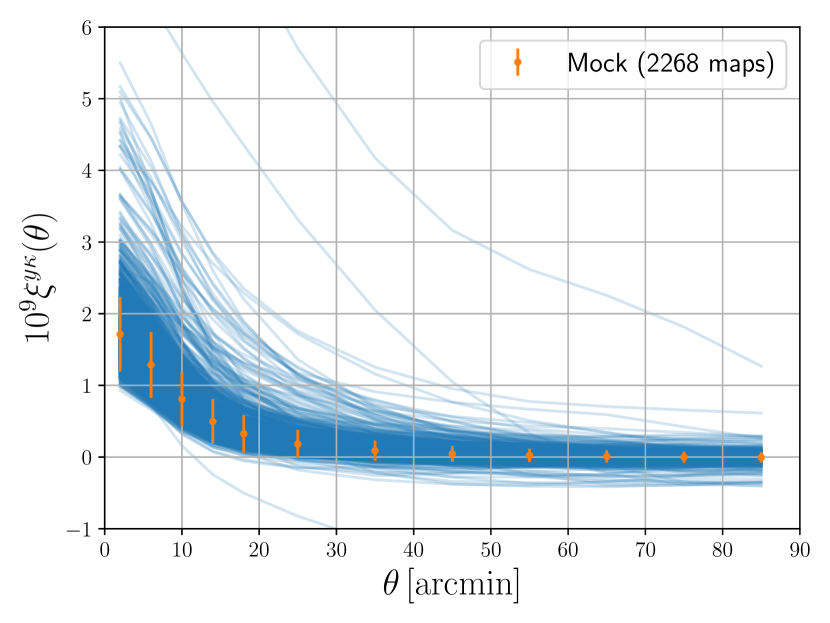
Figure 7: The cross-correlations measured from mock Compton-$y$ and convergence maps. Each blue solid line corresponds to one measurement with a mock map. The orange points with error bars show the mean and standard deviation among 2268 mock maps.

6 Measurement

In this Section, we describe the analysis method of the cross-correlation from the observational data from HSC S16A and Planck.

6.1 Cross-correlations of tSZ and WL

We measure the tSZ-WL cross-correlation function with the following estimator:

$$\hat{\xi}^{y\kappa}(\theta_{k}) = \frac{\sum_{i,j}(\kappa(\bm{\vartheta}_{i})-\kappa_{0})(y(\bm{\vartheta}_{j})-y_{0})w_{ij}(\theta_{k})}{\sum_{i,j}w_{ij}(\theta_{k})},$$ (42)

$$w_{ij}(\theta_{k}) \equiv \frac{1}{\sigma_{\kappa}^{2}(\bm{\vartheta})}B(|\bm{\vartheta}_{i}-\bm{\vartheta}_{j}|,\theta_{k})\mathcal{W}_{\kappa}(\bm{\vartheta}_{i})\mathcal{W}_{y}(\bm{\vartheta}_{j}),$$ (43)

where the subscript $k$ denotes the label of the angular bin. The function $B(\vartheta;\theta)$ denotes the binning scheme, whose configuration is shown in Table 2. The quantities $\kappa_{0}$ and $y_{0}$ are the mean convergence computed for each patch and mean Compton-$y$ in the MILCA Compton-$y$ map, respectively. We apply the inverse variance weight $1/\sigma_{\kappa}^{2}(\bm{\vartheta})$ for convergence and equal weight for Compton-$y$. The variance map for convergence field is estimated as follows. First, we randomly rotate the ellipticity of galaxies in the shape catalog and then reconstruct the convergence field with KS inversion. We repeat this operation $300$ times and generate $300$ convergence maps. The variance $\sigma_{\kappa}^{2}(\bm{\vartheta})$ is computed as the sample variance among these $300$ $E$-mode convergence maps. It is also possible to apply the inverse variance weight for the Compton-$y$ map because the variance map is also provided by the Planck collaboration. However, the high variance region has already been masked and both of the weighting schemes yield consistent results. Therefore, we adopt the equal weight for Compton-$y$. The survey window functions $\mathcal{W}_{\kappa}(\bm{\theta})$ and $\mathcal{W}_{y}(\bm{\theta})$ take zero when the angular position $\bm{\theta}$ is masked and otherwise unity. The mask of Compton-$y$ map is composed of $40\%$ galactic mask and point source mask, and convergence field is masked for the positions where the smoothed galaxy number density is less than the half of the mean density in each patch. We subtract the mean signal for convergence because the KS inversion cannot reconstruct the uniform signal. We also subtract the mean Compton-$y$ because the mean of the mock Compton-$y$ map does not vanish by nature, but the subtraction does not affect the measurement with the real data because the mean is already close to zero due to noise. The means are computed as

$$\kappa_{0} = \frac{\int d^{2}\theta\,\mathcal{W}_{\kappa}(\bm{\theta})\kappa(\bm{\theta})}{\int d^{2}\theta\,\mathcal{W}_{\kappa}(\bm{\theta})},$$ (44)

$$y_{0} = \frac{\int d^{2}\theta\,\mathcal{W}_{y}(\bm{\theta})y(\bm{\theta})}{\int d^{2}\theta\,\mathcal{W}_{y}(\bm{\theta})}.$$ (45)

Instead of using cross-power spectrum directly, we calculate the cross-correlations, in which we can incorporate the masking effect in a straightforward way. To derive the prediction of the cross-correlation, the Hankel transformation is applied to the cross-power spectrum based on halo model:

$$\xi^{y\kappa}(\theta)=\int\frac{\ell d\ell}{2\pi}C^{y\kappa}(\ell)\tilde{W}_{\mathrm{G}}(\ell;\theta_{s}^{\kappa})\tilde{W}_{\mathrm{G}}(\ell;\theta_{s}^{y})J_{0}(\ell\theta),$$ (46)

where $\tilde{W}_{\mathrm{G}}(\ell;\theta_{s})$ is the Fourier transform of the Gaussian window function:

$$\tilde{W}_{\mathrm{G}}(\ell;\theta_{s})=\exp\left(-\frac{1}{4}\ell^{2}\theta_{s}^{2}\right).$$ (47)

In Figure 8, the measurement of the cross-correlation function for each patch in HSC S16A and the radio foreground contribution (see Section 7.1) are shown. Note that the error bar corresponds to the standard deviation for the all HSC S16A regions. That is why the measured cross-correlation for each patch looks statistically inconsistent with the measurement for the all patches but we confirm that the variances are within the statistical uncertainty when the error are scaled according to the area of each patch.

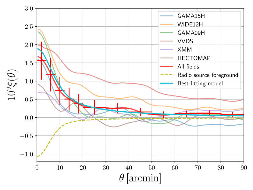
Figure 8: The cross-correlations measured from the Planck Compton-$y$ map and HSC S16A convergence field. The red error bars are estimated from mock measurements. Each thin solid line corresponds to measurement in six different HSC S16A survey patches. The dashed line shows the radio foreground contribution based on halo model in Shirasaki (2019) with the best-fit parameter $B_{\mathrm{R}}$ and the solid cyan line shows the best-fitting halo model prediction, where best-fit parameters are inferred from the cross only data set with the Planck prior (see Section C).

Table 2: The binning of angular separations, the cross-correlations measured with Planck and HSC S16A, the standard deviation estimated from mock observations, and templates for radio source contributions (Shirasaki, 2019).

$\theta_{\mathrm{min}}\,[\mathrm{arcmin}]$	$\theta_{\mathrm{max}}\,[\mathrm{arcmin}]$	$\theta\,[\mathrm{arcmin}]$	$10^{9}\xi^{y\kappa}(\theta)$	$10^{9}\sigma^{y\kappa}(\theta)$	$10^{9}\xi_{\mathrm{R}}(\theta)$
$0.0$	$4.0$	$2.0$	$1.559815$	$0.521110$	$-0.775484$
$4.0$	$8.0$	$6.0$	$1.175148$	$0.458264$	$-0.476844$
$8.0$	$12.0$	$10.0$	$0.736128$	$0.378507$	$-0.220432$
$12.0$	$16.0$	$14.0$	$0.505716$	$0.312014$	$-0.109852$
$16.0$	$20.0$	$18.0$	$0.376050$	$0.261536$	$-0.070340$
$20.0$	$30.0$	$25.0$	$0.279293$	$0.196774$	$-0.045258$
$30.0$	$40.0$	$35.0$	$0.258154$	$0.139731$	$-0.031025$
$40.0$	$50.0$	$45.0$	$0.153550$	$0.108164$	$-0.023614$
$50.0$	$60.0$	$55.0$	$0.075866$	$0.092662$	$-0.018867$
$60.0$	$70.0$	$65.0$	$0.106327$	$0.085000$	$-0.015500$
$70.0$	$80.0$	$75.0$	$0.116000$	$0.077772$	$-0.012971$
$80.0$	$90.0$	$85.0$	$0.075386$	$0.069763$	$-0.011004$

6.2 Null tests

In order to confirm the cross-correlation signal is significant and is not spurious due to systematic effects, we measure the cross-correlation of Compton-$y$ map and auxiliary maps of $B$-mode convergence, PSF leakage, and PSF residual. All of the cross-correlations should be consistent with null detections. The $B$-mode convergence is obtained through the regular analysis and it corresponds to the imaginary part of the convergence field obtained by the KS inversion. In the estimator of the cross-correlation for the $B$-mode map, we need the inverse variance for each pixel as the weight. The variance is estimated from 300 randomly rotated maps, which are also used to estimate the variance in the $E$-mode case. Then, the variance is computed from the imaginary part of convergence field reconstructed from randomly rotated maps. The shape catalog also provides the model estimate of PSF ellipticity $e_{\mathrm{p}}$ at positions of source galaxies. Then, we carry out the KS inversion from the PSF estimates, and cross-correlate it with the Compton-$y$ map. For PSF residual, we can obtain the true PSF from images of stars, which are reserved for the PSF estimation (Bosch et al., 2018), and take the difference of the true PSF and model estimates, $e_{\mathrm{q}}\equiv e_{\mathrm{p}}-e_{\mathrm{star}}$. Similarly to PSF ellipticity $e_{\mathrm{p}}$, we repeat KS inversion and cross-correlation measurements with PSF residual $e_{\mathrm{q}}$. For the cross-correlation measurements with PSF leakage and PSF residual, we adopt equal weight in the estimator instead of inverse variance.

In order to evaluate the statistical significance, i.e., $p$-value, with respect to null signals, we make use of mock Compton-$y$ maps again. We measure the cross-correlations between $B$-mode, PSF leakage, and PSF residual map, and mock Compton-$y$ map $2268$ times. Since these auxiliary maps and mock maps should be uncorrelated, null signals with statistical variance are expected. Then, we compute the chi-square for each measurement:

$$\chi^{2}_{r}=\sum_{i,j}\xi_{r}(\theta_{i})\mathrm{Cov}^{-1}_{ij}\xi_{r}(\theta_{j})\ (r=1,\ldots,2268),$$ (48)

where the covariance matrix is estimated from $2268$ mock measurements. The $p$-value is defined as the number of mock measurements which exceed the chi-square computed with real data. Table 3 shows $p$-values for $B$-mode, PSF leakage, and PSF residual, and we show the cross-correlation measurements between mock Compton-$y$ maps and convergence fields from $B$-mode, PSF leakage, and PSF residual in Figure 9. The $p$-value for each null test is $4.14\%$ ($B$-mode), $17.68\%$ (PSF leakage), and $4.10\%$ (PSF residual), which corresponds to $1.73\sigma$ ($B$-mode), $0.93\sigma$ (PSF leakage), and $1.74\sigma$ (PSF residual) for Gaussian distribution. Thus, we can conclude that the measurements with these three maps are consistent with null signals.

Table 3: The $p$-values for null tests of $B$-mode, PSF leakage, and PSF residual, which are estimated with mock measurements. The corresponding variances for Gaussian distribution are also shown.

Map for null test	$p$-value
$B$-mode	$4.14\%$ ($1.73\sigma$)
PSF leakage	$17.68\%$ ($0.93\sigma$)
PSF residual	$4.10\%$ ($1.74\sigma$)

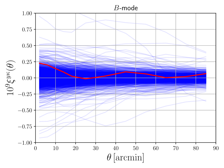
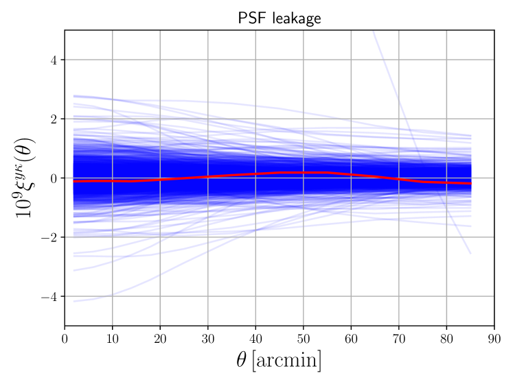
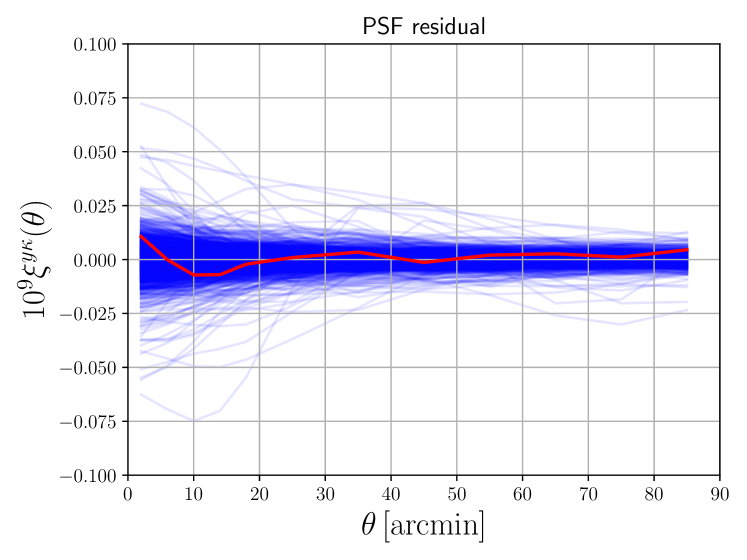
Figure 9: The cross-correlations with $B$-mode, PSF leakage, and PSF residual maps and real or mock Compton-$y$ maps. The red line is the measurement with real data. There are 2268 blue lines, each of which corresponds to the measurement with one mock Compton-$y$ map.

6.3 Statistical significance of the measurement

Here, we evaluate the statistical significance of the $E$-mode signal. Similarly to the null tests, we carry out cross-correlation measurements with $E$-mode convergence and mock Compton-$y$ maps, and compute chi-square for each measurement. Figure 10 shows the real measurement with and without foreground subtraction and mock measurements with real and mock Compton-$y$ maps. It is expected that the mock measurement should be null because we cross-correlate the real convergence map and the mock Compton-$y$ maps in contrast to measurements with mock convergence maps and mock Compton-$y$ maps (see Figure 7), where the significant signal is expected. The $p$-value corresponds to the fraction of mock measurements which chi-square exceeds the one from the true measurement. The derived $p$-value for the $E$-mode cross-correlation is $0.0441\%$, which corresponds to $3.33\sigma$ for Gaussian distribution. On the other hand, the $E$-mode cross-correlation contains the contamination due to foreground radio emission. We subtract the contribution from the measured $E$-mode cross-correlation with the best-fit amplitude parameter $B_{\mathrm{R}}$ (see Section 7.1 and Eq. 50) inferred with the cross only data set with the Planck prior (see Section 7.2). After the foreground removal, we then recompute the chi-square with respect to null signal. The resultant $p$-value is $2.38\%$, which corresponds to $1.98\sigma$ for Gaussian distribution.

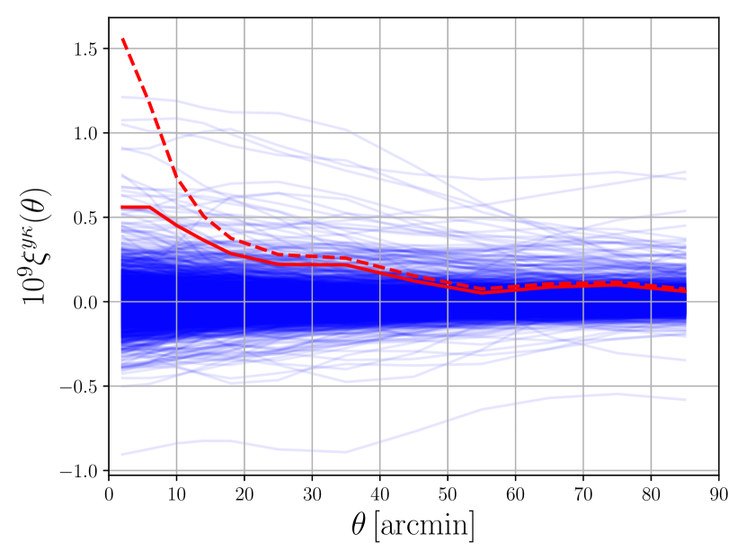
Figure 10: The cross-correlations with $E$-mode map and real or mock Compton-$y$ maps. The red solid line is the real measurement with the radio contribution subtracted with the best-fit parameter $B_{\mathrm{R}}$, which is inferred from the cross only data set with the Planck prior (see Appendix C). The real measurement before subtraction of the radio contribution is also shown as the red dashed line. There are 2268 blue lines, each of which corresponds to measurement with one mock Compton-$y$ map.

7 Cosmological analyses

7.1 Foreground contribution

Due to imperfect separation of foreground components in constructing Compton-$y$ map, the measured auto-power spectrum and cross-correlations contain the contribution from the foreground. Such foregrounds include cosmic infrared background (CIB), radio point sources, and infrared point sources. In our analysis, we take into account these contributions following Bolliet et al. (2018) for the tSZ auto-power spectrum and Shirasaki (2019) for the tSZ-WL cross-correlation.

First, we briefly describe the foreground treatment in the auto-power spectrum in Bolliet et al. (2018). They consider three foreground contributions: CIB, radio point sources (RS), and infrared point sources (IR). In addition to these components, the residual correlated noise (CN) is also included. The power spectrum templates for these components are given in Planck Collaboration et al. (2016a). The amplitudes of the power spectra are modelled as nuisance parameters, and in summary, the total power spectrum $\hat{C}^{yy}$ is given as

$$\hat{C}^{yy}(\ell) = C^{yy}(\ell)+A_{\mathrm{CIB}}C_{\mathrm{CIB}}(\ell)+A_{\mathrm{IR}}C_{\mathrm{IR}}(\ell)+$$ (49)

$$A_{\mathrm{RS}}C_{\mathrm{RS}}(\ell)+A_{\mathrm{CN}}C_{\mathrm{CN}}(\ell),$$

where $C^{yy}$ is the prediction based on halo model, $C_{\mathrm{CIB}}$, $C_{\mathrm{IR}}$, $C_{\mathrm{RS}}$, and $C_{\mathrm{CN}}$ are templates for CIB, IR, RS, and CN, respectively. The amplitude of CN $A_{\mathrm{CN}}$ is determined with the measurement at the highest multipole ($\ell=2742$) because the CN term is dominant at small scales. As a result, we fix the amplitude of the CN term as $A_{\mathrm{CN}}=\hat{C}^{yy}(\ell=2742)/C_{\mathrm{CN}}(\ell=2742)=0.903$. Other amplitudes ($A_{\mathrm{CIB}}$, $A_{\mathrm{IR}}$, and $A_{\mathrm{RS}}$) are treated as nuisance parameters and marginalized in subsequent analysis. The template power spectrum and total tSZ auto-power spectrum is shown in Figure 11 and Table 4.

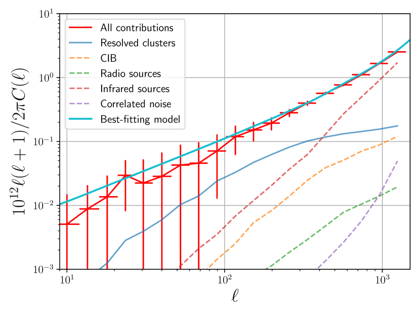
Figure 11: The auto-power spectra of tSZ measured from Planck and templates for the foreground contributions of CIB, RS, and IR, and the correlated noise contribution. The amplitude of the correlated noise is $A_{\mathrm{CN}}=0.903$. The solid cyan line shows the best-fitting halo model prediction and the dashed lines show the best-fitting foreground power spectra where best-fit parameters are inferred from the auto only data set with the Planck prior (see Appendix C). The contribution from resolve clusters is also shown as the blue solid line. The red error bars are estimated from mock measurements.

Table 4: The binning of multipoles, the auto-power spectrum measured by Planck, the standard deviation estimated from mock observations, the templates for CIB, RS, and IR, the contributions of CN and resolved clusters (RC). All of the template power spectra are based on Bolliet et al. (2018). Instead of the raw power spectrum $C(\ell)$, the band-power $D(\ell)\equiv\ell(\ell+1)/(2\pi)C(\ell)$ is shown. Note that the largest multipole bin ($\ell=1247.5$) is used only in Eq. (58).

$\ell_{\mathrm{min}}$	$\ell_{\mathrm{max}}$	$\ell$	$10^{12}D^{yy}(\ell)$	$10^{12}\sigma^{yy}(\ell)$	$10^{12}D_{\mathrm{RC}}(\ell)$	$10^{12}D_{\mathrm{CIB}}(\ell)$	$10^{12}D_{\mathrm{RS}}(\ell)$	$10^{12}D_{\mathrm{IR}}(\ell)$	$10^{12}D_{\mathrm{CN}}(\ell)$
$9$	$12$	$10.0$	$0.005080$	$0.009812$	$0.000421$	$0.000000$	$0.000043$	$0.000007$	$0.000001$
$12$	$16$	$13.5$	$0.008810$	$0.011924$	$0.000710$	$0.000000$	$0.000142$	$0.000024$	$0.000001$
$16$	$21$	$18.0$	$0.013630$	$0.015646$	$0.001251$	$0.000000$	$0.000296$	$0.000048$	$0.000002$
$21$	$27$	$23.5$	$0.029610$	$0.021492$	$0.002837$	$0.000000$	$0.000400$	$0.000073$	$0.000004$
$27$	$35$	$30.5$	$0.022410$	$0.030094$	$0.003933$	$0.000902$	$0.000541$	$0.000111$	$0.000006$
$35$	$46$	$40.0$	$0.028490$	$0.038872$	$0.005969$	$0.002010$	$0.001056$	$0.000224$	$0.000010$
$46$	$60$	$52.5$	$0.042760$	$0.046322$	$0.010318$	$0.003119$	$0.001647$	$0.000449$	$0.000018$
$60$	$78$	$68.5$	$0.045800$	$0.051503$	$0.014045$	$0.006278$	$0.002787$	$0.000837$	$0.000030$
$78$	$102$	$89.5$	$0.071040$	$0.058284$	$0.024061$	$0.012242$	$0.004306$	$0.001400$	$0.000052$
$102$	$133$	$117.0$	$0.119140$	$0.057526$	$0.032976$	$0.021584$	$0.006842$	$0.002701$	$0.000089$
$133$	$173$	$152.5$	$0.151500$	$0.051520$	$0.047100$	$0.045915$	$0.011264$	$0.004721$	$0.000153$
$173$	$224$	$198.0$	$0.193900$	$0.045036$	$0.062380$	$0.070582$	$0.016744$	$0.008115$	$0.000262$
$224$	$292$	$257.5$	$0.281750$	$0.039697$	$0.081730$	$0.119786$	$0.027345$	$0.014618$	$0.000456$
$292$	$380$	$335.5$	$0.398370$	$0.036168$	$0.101911$	$0.211686$	$0.043275$	$0.024893$	$0.000815$
$380$	$494$	$436.5$	$0.567430$	$0.033381$	$0.117412$	$0.332863$	$0.070587$	$0.051570$	$0.001503$
$494$	$642$	$567.5$	$0.768660$	$0.032938$	$0.132234$	$0.434931$	$0.115356$	$0.107293$	$0.002934$
$642$	$835$	$738.0$	$1.110100$	$0.031719$	$0.143214$	$0.602030$	$0.154926$	$0.197053$	$0.006334$
$835$	$1085$	$959.5$	$1.661400$	$0.027203$	$0.156202$	$0.754733$	$0.207200$	$0.361713$	$0.016171$
$1085$	$1411$	$1247.5$	$2.521700$	$0.030189$	$0.175341$	$1.029014$	$0.287652$	$0.681036$	$0.054883$

Next, we discuss the foreground contribution in the tSZ-WL cross-correlations. We employ the halo model prescription proposed in Shirasaki (2019), where the template cross-power spectrum from extragalactic radio sources: flat-spectrum radio quasars, BL Lac objects, and steep-spectrum sources. Shirasaki (2019) also addresses the contribution from CIB, but we do not include the contribution because the effect due to CIB is subdominant for the cross-correlation. The template is computed with respect to the radio frequency, and to convert them into Compton-$y$, we employ the weight of Map C in Table 1 of Van Waerbeke et al. (2014). The template is shown in Table 2. Since the weighting scheme is different for the MILCA Compton-$y$ map, we introduce the amplitude parameter $B_{\mathrm{R}}$ and treat it as a nuisance parameter in the analysis. As a result, the total cross-correlation $\hat{\xi}^{y\kappa}$ is given as

$$\hat{\xi}^{y\kappa}(\theta)=\xi^{y\kappa}(\theta)+B_{\mathrm{R}}\xi_{\mathrm{R}}(\theta),$$ (50)

where $\xi^{y\kappa}(\theta)$ is the predicted cross-correlation based on halo model.

7.2 Inference of parameters

In the analysis, we use tSZ-WL cross-correlations from HSC and Planck and tSZ auto-power spectrum from Planck in order to constrain cosmological parameters and the hydrostatic bias parameter $b_{\mathrm{HSE}}$.

First, we define the data vector as

$$D_{C} = (C^{yy}(\ell_{1}),\ldots,C^{yy}(\ell_{n_{C}})),$$ (51)

$$D_{\xi} = (\xi^{y\kappa}(\theta_{1}),\ldots,\xi^{y\kappa}(\theta_{n_{\xi}})),$$ (52)

$$D_{C+\xi} = (D_{C},D_{\xi}),$$ (53)

where $n_{C}=18$ and $n_{\xi}=12$ are the number of bins in auto-power spectrum and cross-correlation, respectively. The binning is shown in Table 4 for the auto-power spectrum and Table 2 for the cross-correlations. Note that the largest multipole bin $\ell=1247.5$ in the auto-power spectrum is used only for the condition Eq. (58). From the mock measurements, we estimate covariance matrix,

$$\mathrm{Cov}_{ij}=\frac{1}{R-1}\sum_{r=1}^{R}(D^{r}_{i}-\bar{D}_{i})(D^{r}_{j}-\bar{D}_{j}),$$ (54)

where $R$ is the number of realizations, $\bar{D}$ is the sample mean of $R$ measurements, and $r=1,\ldots,R$ denotes the label of the realization. There are $R=108$ maps for mock Compton-$y$ and $R=2268$ maps for mock convergence. As a result, we have 108 and 2268 measurements of auto-power spectrum and cross-correlations, respectively. For estimation of cross-covariance between auto-power spectrum and cross-correlation, we additionally generate $2268$ maps for Compton-$y$ by rotating the coordinates to adjust the one in mock convergence map. These additional mock Compton-$y$ maps are used for cross-covariance estimation, null tests, and evaluation of significance of cross-correlations. The estimated covariance matrix of the tSZ auto-power spectrum and the tSZ-WL cross-correlation is shown in Figure 12.

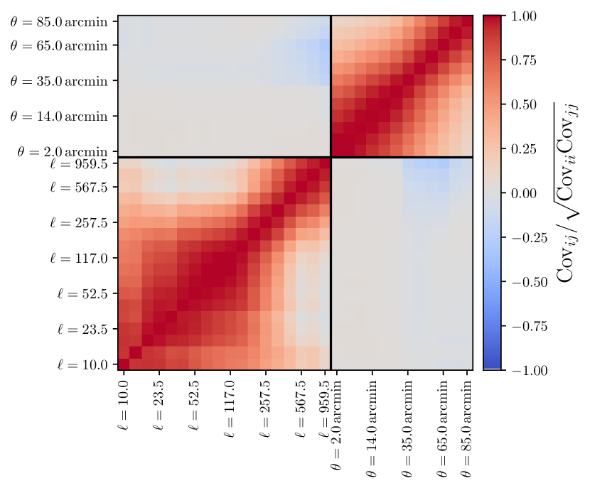
Figure 12: Covariance matrix of the tSZ auto-power spectrum and the tSZ-WL cross-correlation estimated from mock observations.

The likelihood $\mathcal{L}$ is assumed to be multivariate Gaussian as

$$\log\mathcal{L}(\bm{p})=-\frac{1}{2}\sum_{i,j}(\hat{D}_{i}-D_{i}(\bm{p}))\mathrm{Cov}^{-1}_{ij}(\hat{D}_{j}-D_{j}(\bm{p}))+\text{const.},$$ (55)

where $\hat{D}$ is the measurement, $D(\bm{p})$ is the prediction based on the halo model, and $\bm{p}$ is the parameter vector, which includes cosmological parameters, hydrostatic bias parameter $b_{\mathrm{HSE}}$, and nuisance parameters. The cosmological parameters are composed of physical baryon density $\omega_{\mathrm{b}}\equiv\Omega_{\mathrm{b}}h^{2}$, physical CDM density $\omega_{\mathrm{cdm}}\equiv\Omega_{\mathrm{cdm}}h^{2}$, scaled Hubble parameter $h\equiv H_{0}/(100\,\mathrm{km}\,\mathrm{s}^{-1}\,\mathrm{Mpc}^{-1})$, tilt and amplitude of the scalar perturbation $n_{\mathrm{s}}$ and $\ln(10^{10}A_{\mathrm{s}})$. In addition, we also consider three derived parameters: the total matter density with respect to critical density, $\Omega_{\mathrm{m}}$, the amplitude of the matter fluctuation at the scale of $8\,h^{-1}\,\mathrm{Mpc}$, $\sigma_{8}$, and the amplitude parameter $S_{8}\equiv\sigma_{8}(\Omega_{\mathrm{m}}/0.3)^{0.5}$, which roughly corresponds to the amplitude of cosmic shear power spectrum or correlation function. Throughout the analysis, we assume the flat $\Lambda$CDM Universe and there are three species of neutrinos, one of which has finite mass of $m_{\nu}=0.06\,\mathrm{eV}$. The total matter density with respect to critical density $\Omega_{\mathrm{m}}$ is the sum of CDM $\Omega_{\mathrm{cdm}}$, baryon $\Omega_{\mathrm{b}}$, and massive neutrinos $\Omega_{\nu}=m_{\nu}/(93.14\,h^{2}\,\mathrm{eV})$. In addition to cosmological parameters, we take the hydrostatic bias parameter $b_{\mathrm{HSE}}$ into account. Nuisance parameters are introduced depending on data sets: for the auto-power spectrum, amplitude parameters of foreground contributions, $A_{\mathrm{CIB}}$, $A_{\mathrm{IR}}$, and $A_{\mathrm{RS}}$, and for the cross-correlation, an amplitude parameter of radio foreground $B_{\mathrm{R}}$. The details on how to estimate the inverse covarince matrix from the sample covariance matrix are found in Appendix B. Only with auto-power spectrum and cross-correlations, the constraining power is weak and it is hard to obtain converged results. Therefore, we add priors on cosmological parameters from external measurements. In this analysis, we consider two priors. One is a combination of results of large-scale structure measurements (hereafter LSS prior): Joint Light-curve Analysis (JLA) of SDSS-II and SNLS for type Ia supernovae (Betoule et al., 2014), Baryon Oscillation Spectroscopic Survey (BOSS) Data Release 12 for baryon acoustic oscillations and redshift space distortions (Alam et al., 2017), and HSC S16A WL cosmic shear power spectrum (Hikage et al., 2019). The other one is the Planck 2018 results in TT,TE,EE+lowE+lensing dataset (Planck Collaboration et al., 2018a, b) (hereafter Planck prior). The LSS prior includes additional four nuisance parameters (see Appendix C).

Hence, the posterior distribution $\mathcal{P}$ is given as

$$\log\mathcal{P}(\bm{p})=\log\mathcal{L}(\bm{p})+\log P(\bm{p})+\text{const}.$$ (56)

We utilize the Markov chain Monte-Carlo code MontePython-3 (Audren et al., 2013; Brinckmann & Lesgourgues, 2018) to obtain chains for the posterior distribution. In order to confirm the convergence of obtained chains, we compute Gelman–Rubin statistic $R$ for all parameters and run the analysis until the condition $R-1<0.01$ is reached. For priors from HSC S16A cosmic shear power spectrum analysis or Planck 2018 results, we assume the multivariate Gaussian form as

$$\log P(\bm{p})=-\frac{1}{2}\sum_{\alpha,\beta}(p_{\alpha}-\bar{p}_{\alpha})\mathcal{C}^{-1}_{\alpha\beta}(p_{\beta}-\bar{p}_{\beta})+\text{const.},$$ (57)

where the mean $\bar{\bm{p}}$ and the covariance matrix $\mathcal{C}_{\alpha\beta}$ are estimated from parameter chains. Note that the deviation from the multivariate Gaussian affects the resultant constraints compared with the one with the full likelihood analysis. For example, in the case with cosmic shear power spectrum, the constraint on the amplitude parameter $S_{8}$ is significantly degraded because the approximation cannot fully capture the shape of the degeneracy between $\sigma_{8}$ and $\Omega_{\mathrm{m}}$. However, it provides the reasonable estimates on the prior of most of parameters. For other data sets (JLA and BOSS), we make use of likelihood packages provided in MontePython-3. For the prior on the hydrostatic bias parameter, we adopt a hard prior $b_{\mathrm{HSE}}<1$, which ensures the hydrostatic mass is positive. In addition, we impose an additional condition on the auto-power spectrum following Bolliet et al. (2018). The contribution from the galaxy clusters which have already been observed in X-ray or SZ has been measured and is shown in Table 4. The prediction should exceed the contribution at least small scales, where the absolute errors are small, i.e.,

$$C^{yy}(\ell)-C_{\mathrm{RC}}(\ell)>0.$$ (58)

This condition should be satisfied for all multipoles between $\ell=257.5$ and $\ell=1247.5$. The power spectrum at large scales has large statistical variances and is not subject to the condition. If this condition is not satisfied, we force posterior to be zero.

We show constraints of parameters with tSZ auto-power spectrum and tSZ-WL cross-correlations for LSS and Planck priors in Figures 13 and 14, respectively. The results in the full parameter space (cosmological parameters, hydrostatic bias, nuisance parameters, and derived parameters) are found in Appendix C. In each case, we present constraints with three data sets: tSZ auto-power spectrum only (hereafter, auto only), tSZ-WL cross-correlation only (cross only), and joint analysis with both of them (joint). Since $b_{\mathrm{HSE}}$ is highly degenerated with cosmological parameters, the tighter constraints can be obtained with Planck prior because this prior determines the cosmological parameters better. As a whole, the constraining power of tSZ auto-power spectrum is better than that of tSZ-WL cross-correlations due to the large survey area. Though errors are large for the case of the cross-correlation only data set, all three data sets give consistent results for all cosmological parameters and $b_{\mathrm{HSE}}$. The constraints with the joint data set do not necessarily lie between the results with the auto only and cross only data sets because of the cross-covariance between the auto-power spectrum and cross-correlation.

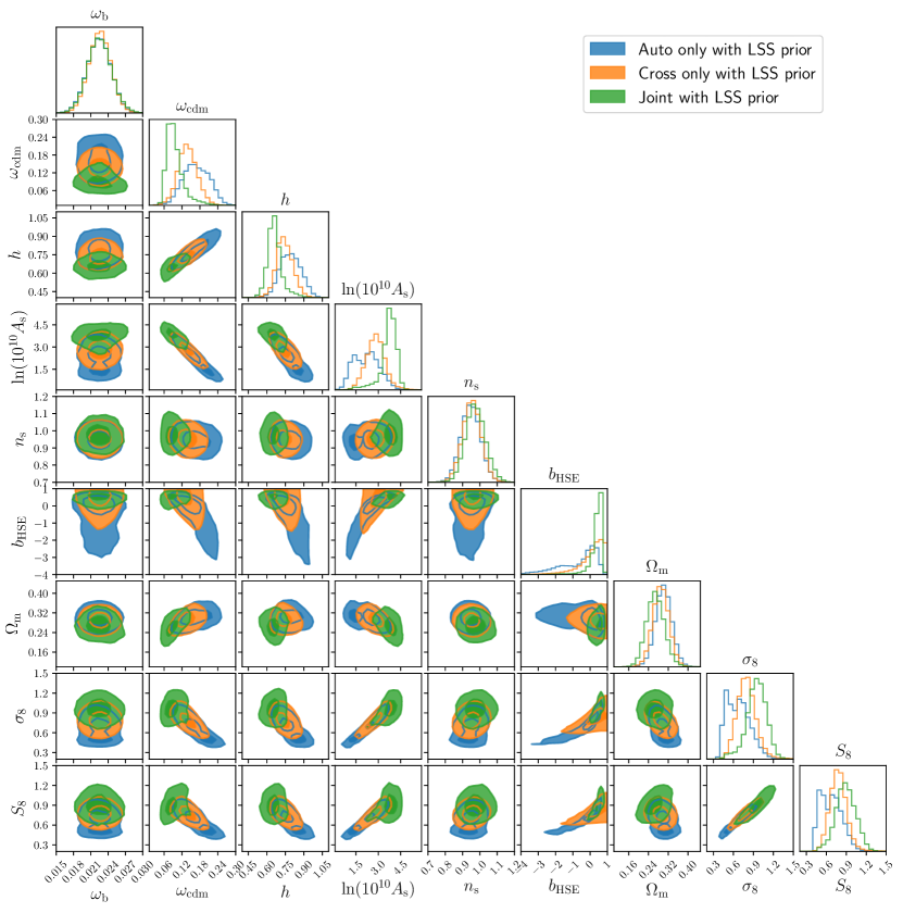
Figure 13: Confidence regions of cosmological parameters and hydrostatic bias parameter inferred with three data sets (auto only, cross only, and joint) with the LSS prior. The inner (outer) contour corresponds to the $1\sigma$ ($2\sigma$) confidence level. The diagonal panels show the marginalized likelihoods.

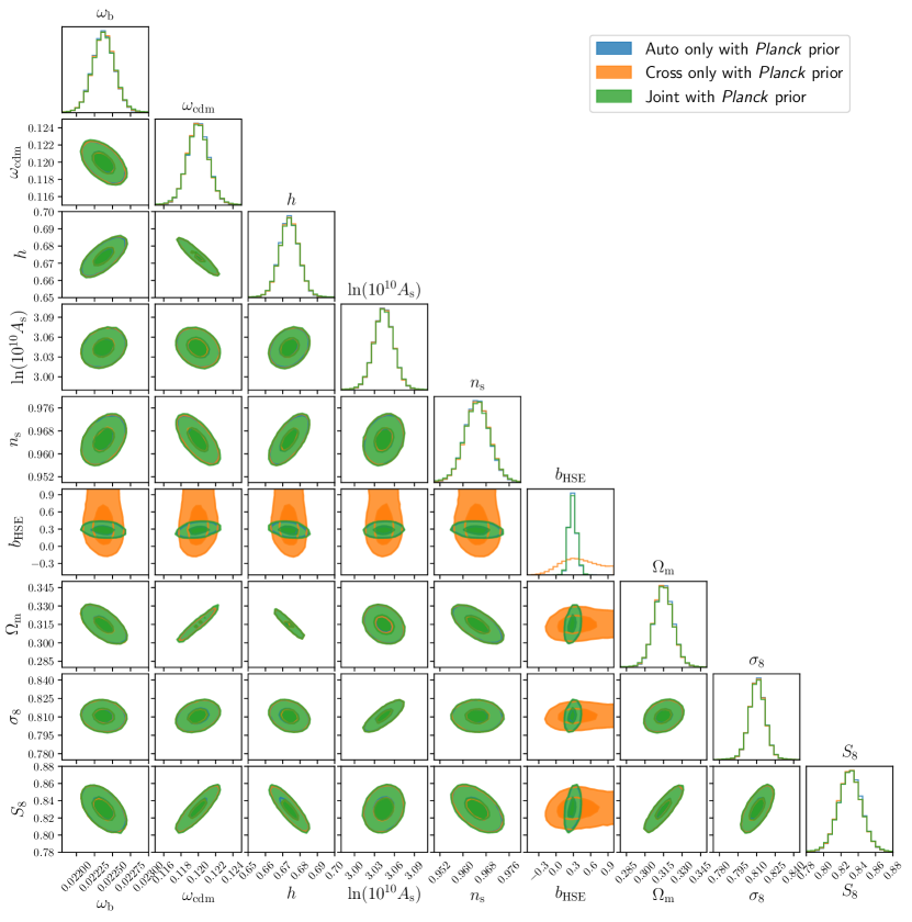
Figure 14: Confidence regions of cosmological parameters and hydrostatic bias parameter inferred with three data sets (auto only, cross only, and joint) with the Planck prior. The inner (outer) contour corresponds to the $1\sigma$ ($2\sigma$) level. The diagonal panels show the marginalized likelihoods.

In Figure 15, the constraints on the amplitude parameter $S_{8}$ and the hydrostatic bias parameter $b_{\mathrm{HSE}}$ are shown. Due to weak constraining power on cosmological parameters of the LSS prior, the error contour for data sets with the prior is much larger than those with the Planck prior, but all of results are consistent with each other and the tightest constraint, which is obtained with auto only or joint data sets with the Planck prior, prefers the amplitude parameter $S_{8}\simeq 0.83$ and the hydrostatic bias parameter $b_{\mathrm{HSE}}\simeq 0.3$.

Figure 15: Confidence regions of hydrostatic bias and amplitude parameter $S_{8}$ for three data sets with two priors. The inner (outer) contour corresponds to the $1\sigma$ ($2\sigma$) level.

8 Discussions

8.1 Contributions from resolved clusters

In order to estimate the contributions from clusters which have already been detected both through HSC WL surveys and Planck SZ observations, we repeat the measurement with the additional mask covering the detected clusters. We use the cluster catalog in Medezinski et al. (2018), which contains $5$ clusters located within the HSC S16A footprints and the SZ signals have already been detected by Planck (Planck Collaboration et al., 2016b). The locations, redshifts, and masses which are inferred by fitting the WL signal with the NFW profile are shown in Table 5. We mask the regions within the angular extent $\theta_{200}=R_{200}/d_{A}(z)$ for each cluster, where $d_{A}(z)$ is the angular diameter distance. In Figure 16, we show the cross-correlations with and without the mask of cluster regions. The difference between two signals corresponds to the contribution from massive clusters which are detected by Planck. Accordingly, the massive clusters can contribute to the signal by at most $\simeq 20\%$, and thus the rest of signal comes from the unresolved, i.e., low-mass, halos. Hence, the cross-correlations contain the information from low-mass halos, which are not easily accessible from other observables.

Table 5: The catalog of SZ detected clusters by Planck which are located in HSC S16A footprints (Medezinski et al., 2018). The mass of clusters is inferred by fitting WL signal assuming the NFW profile. The positions of clusters are defined as those of brightest central galaxies.

Name in Planck SZ catalog	NED name	RA (J2000)	Dec (J2000)
PSZ2 G068.61-46.60	Abell 2457	$22^{\mathrm{h}}35^{\mathrm{m}}40\aas@@fstack{s}80$	$+01\degr 29\arcmin 05\aas@@fstack{\prime\prime}60$
PSZ2 G167.98-59.95	Abell 0329	$02^{\mathrm{h}}14^{\mathrm{m}}41\aas@@fstack{s}09$	$-04\degr 34\arcmin 02\aas@@fstack{\prime\prime}46$
PSZ2 G174.40-57.33	Abell 0362	$02^{\mathrm{h}}31^{\mathrm{m}}41\aas@@fstack{s}17$	$-04\degr 52\arcmin 57\aas@@fstack{\prime\prime}29$
PSZ2 G228.50+34.95	MaxBCG J140.53188+03.76632	$09^{\mathrm{h}}22^{\mathrm{m}}10\aas@@fstack{s}96$	$+03\degr 46\arcmin 41\aas@@fstack{\prime\prime}52$
PSZ2 G231.79+31.48	MACS J0916.1-0023/Abell 0776	$09^{\mathrm{h}}16^{\mathrm{m}}09\aas@@fstack{s}24$	$-00\degr 24\arcmin 16\aas@@fstack{\prime\prime}31$

Redshift $z$	Mass $M_{\mathrm{200}}$ [$10^{14}\,h^{-1}\,\mathrm{M}_{\sun}$]	Radius $R_{\mathrm{200}}$ [$h^{-1}\,\mathrm{Mpc}$]	Angular extent $\theta_{200}$ [$\mathrm{arcmin}$]
$0.0594$	$2.02$	$0.938$	$19.43$
$0.1393$	$2.21$	$0.943$	$9.12$
$0.1843$	$4.12$	$1.144$	$8.79$
$0.2701$	$31.03$	$2.177$	$12.48$
$0.3324$	$8.10$	$1.361$	$6.75$

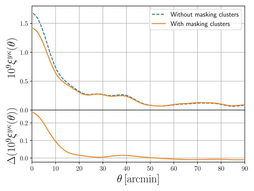
Figure 16: The cross-correlations with (solid line) and without (dashed line) SZ-detected clusters in HSC S16A survey footprints masked (Medezinski et al., 2018). The lower panel shows the difference between these two measurements.

8.2 Comparison with mass calibration measurements

Here, we discuss the implications of the results, especially the constraints on the hydrostatic bias. The constraints on the hydrostatic bias parameter is summarized in Table 6. As we have seen, the constraints on the bias parameter strongly depend on priors. Here, we focus on the result with the Planck prior because previous works of mass calibration measurements and hydrodynamical simulations also adopt Planck cosmology or similar one.

When the auto only or joint data sets are used, the resultant constraint on the hydrostatic bias parameter is $b_{\mathrm{HSE}}\simeq 0.3$, which is consistent with the hydrostatic mass bias of $0.1\text{--}0.3$ derived using X-ray/SZ and WL mass measurements of individual clusters. In the case with the cross only data set, a slightly higher hydrostatic bias parameter ($b_{\mathrm{HSE}}\simeq 0.32$) is preferred, although the error is large. We note that the analysis of the tSZ auto-power spectrum by Bolliet et al. (2018) also suggests a higher hydrostatic bias of $\simeq 40\%$. We compare the obtained results and the previous mass calibration measurements in Figure 17. Note that the tSZ auto-power spectrum and tSZ-WL cross-correlation are sensitive to wide ranges of the halo mass (see Section 2.4) and thus the hydrostatic mass bias is not uniformly constrained with respect to mass.

One of the possibilities to explain the discrepancy between cross only and other data sets is varying sensitivity to the halo mass and redshift range of these measurements. Although the signal of tSZ auto-power spectrum comes from galaxy clusters and groups with a wide range of mass (see, e.g., Makiya et al., 2018), mass calibration measurements probe only into massive clusters. As Figure 1 shows, the tSZ-WL cross-correlation is sensitive to the structures at higher redshifts compared to the tSZ auto-power spectrum (see also Battaglia et al., 2015). Thus, the discrepancy demonstrates non-thermal pressure depends on redshift or mass. This hypothesis will be confirmed once the cross-correlations are measured for larger areas and the constraints become tighter.

8.3 Comparison with simulation predictions

Current observational constraints on the hydrostatic mass bias are broadly consistent with the predictions of hydrodynamical simulations (e.g., Nagai et al., 2007b; Lau et al., 2009; Nelson et al., 2014a; Shi et al., 2016; Biffi et al., 2016; Henson et al., 2017). However, we emphasize that the predicted hydrostatic mass bias in the literature ranges from 15 to 40% depending the halo mass, and even depending on the numerical codes and methods used. Further studies of the nature and origin of the hydrostatic mass bias are clearly required. In particular, it is important to understand the non-thermal pressure contributing to the HSE equation (Lau et al., 2013), the effects of mass- and code-dependent temperature inhomogeneities effect on the X-ray spectral temperature (Rasia et al., 2014), the role of acceleration term (Suto et al., 2013; Nelson et al., 2014a), and the redshift evolution of the non-thermal pressure and the HSE mass bias.

Table 6: Constraints on the hydrostatic parameter for each data set. The central values are best-fit in each analysis and the errors correspond to $68\%$ C.L., which are estimated from parameter chains.

Data set	LSS prior	Planck prior
Auto only	$0.306^{+0.001}_{-2.268}$	$0.237^{+0.118}_{-0.010}$
Cross only	$0.334^{+0.433}_{-0.390}$	$0.320^{+0.437}_{-0.236}$
Joint	$0.260^{+0.380}_{-0.105}$	$0.269^{+0.089}_{-0.044}$

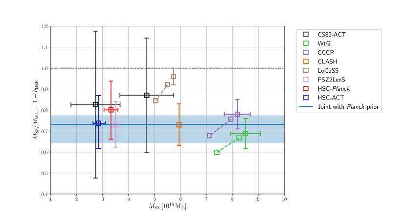
Figure 17: The comparison of hydrostatic bias parameters with respect to the hydrostatic mass $M_{\mathrm{SZ}}$ obtained with WL mass calibration measurements. The results with the joint data set of the tSZ auto-power spectrum and the tSZ-WL cross-correlations with the Planck prior is shown as blue bands, which correspond to 68% confidence level, and the blue solid line corresponds to the best-fit value. The results in CS82-ACT (Battaglia et al., 2016), LoCuSS (Smith et al., 2016), CLASH (Penna-Lima et al., 2017), PSZ2LenS (Sereno et al., 2017), HSC-Planck (Medezinski et al., 2018) and HSC-ACT (Miyatake et al., 2019) are shown as black, brown, orange, pink, red, and blue squares, respectively. The green and purple squares show the results in WtG (von der Linden et al., 2014) and CCCP (Hoekstra et al., 2015), respectively, and the same colored squares connected with dashed lines are results where the Eddington bias are corrected by the level of $3\text{--}15\%$ computed in Battaglia et al. (2016). In the LoCuSS measurement, the Eddington bias is estimated in von der Linden et al. (2014) and the corrected result is shown as the brown square connected with dashed lines.

9 Conclusions

We present measurements of cross-correlations of WL and tSZ from HSC S16A and Planck data and derive constraints on cosmological parameters and hydrostatic bias parameter using the tSZ auto-power spectrum and the tSZ-WL cross-correlations. For WL, we reconstruct the convergence field from HSC S16A shape catalog (Mandelbaum et al., 2018a), which covers $136.9\,\mathrm{deg}^{2}$ with the mean number density $n_{g}=24.6\,\mathrm{arcmin}^{-2}$. For tSZ, we make use of the Compton-$y$ map based on MILCA algorithm from $30$ to $857$ GHz channel maps of Planck data (Planck Collaboration et al., 2016a). To calculate the auto-power spectrum and cross-correlation, we use the halo model prescription with the universal pressure profile (Nagai et al., 2007b). To calibrate the universal pressure profile, the clusters are assumed to be in HSE, and thus the true mass may be larger than the estimated mass under HSE because non-thermal pressure support by turbulent motions and other physical processes may be strong. In order to account for the non-thermal pressure support, we introduce the hydrostatic mass bias parameter $b_{\mathrm{HSE}}$, which denotes the fraction of mass supported by non-thermal pressure, and rescale the mass and the radius in the universal pressure profile. For accurate estimation of covariance matrix, We create realistic mock tSZ maps from all-sky $N$-body simulations (Takahashi et al., 2017) and use them to estimate the data covariance matrix accurately. In addition to the mock tSZ maps, we also utilize the mock shape catalog, which is created from the HSC S16A shape catalog (Shirasaki et al., 2019). The various systematic effects specific to the HSC observation, e.g., survey masks and discrete distribution of source galaxies, are incorporated in a direct manner. Then, we compute the auto-power spectrum and cross-correlation from the suite of mock maps, and estimate the covariance matrix. Using the observational data and the covariance matrix estimated from our 2268 mock catalogues, we perform statistical analysis to constrain the cosmological parameters and the hydrostatic bias parameter with the tSZ auto-power spectrum and the tSZ-WL cross-correlation. We add priors on cosmological parameters from the combinations of results from measurements of JLA (Betoule et al., 2014), BOSS (Alam et al., 2017), and HSC cosmic shear analysis (Hikage et al., 2019), or Planck 2018 results of the temperature and polarization anisotropies of CMB and CMB lensing (Planck Collaboration et al., 2018a, b). The hydrostatic bias parameter is strongly degenerate with cosmological parameters, and thus the constraints depend on the choice of the priors. In the case of using data sets with tSZ auto-power spectrum only or joint analysis of tSZ auto-power spectrum and tSZ-WL cross-correlations with the Planck prior, we find a reasonable value of the hydrostatic bias parameter $\simeq 30\%$, which is consistent with WL mass calibration measurements (e.g., Miyatake et al., 2019) and the joint analysis of power spectra of cosmic shear with HSC and tSZ with Planck (Makiya et al., 2019). On the other hand, when the data set only with tSZ-WL cross-correlations is employed, slightly higher hydrostatic bias parameter ($\simeq 32\%$) is estimated. Because both of tSZ power spectrum and tSZ-WL cross-correlations can probe into less massive halos ($\lesssim 10^{14}\,\mathrm{M}_{\sun}$), which are not accessible both for mass calibration measurements and hydrodynamical simulations, the higher value of the hydrostatic bias can be realized by high non-thermal pressure support in such less massive halos. Since the HSC regions are limited to small sky coverage of $\sim 100\,\mathrm{deg}^{2}$, the constraint is not so tight, but for full sky coverage $\sim 1000\,\mathrm{deg}^{2}$, tighter constraints can be obtained, and it will be possible to probe into the redshift evolution of non-thermal pressure support via inference of hydrostatic bias by a tomographic technique. Furthermore, the ground-based CMB observatories, e.g., ACT and SPT, are operating and Stage-IV CMB experiments will start operation in the near future. The tSZ observations with high resolution and image quality by these experiments enable one to utilize small scale ($<1\,\mathrm{arcmin}$) measurements, which are useful to address the fine structure of the pressure profile of galaxy clusters. Considering the large overlapping areas with HSC, it is expected that we can fully trace the redshift evolution and mass dependence of the non-thermal pressure at high precision with the upcoming ground-based CMB experiments.

Appendix A Effects of choice of algorithms in photometric redshifts estimation

We show the dependence on algorithms of photometric redshift estimation for the cross-correlation calculations. Figure 18 shows the halo model calculations with WMAP 9-yr cosmological parameters (see Section 5) for eight different stacked PDFs. The difference from the fiducial model, i.e., the one with Ephor AB with reweights of COSMOS 30-band observations, is within $2\%$ at all scales.

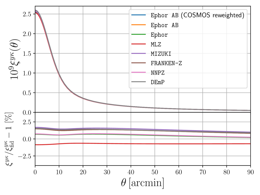
Figure 18: The cross-correlations based on halo model with different codes of photometric redshift estimation. The lower panel shows the fractional difference from the fiducial cross-correlation, i.e., the one with Ephor AB with reweights of COSMOS 30-band observations.

Appendix B Estimator of inverse covariance matrix

In the case of dealing with correlated and high dimensional data, to compute the inverse covariance matrix, standard inversion of estimated covariance matrix $S$ may lead to numerically unstable estimation of the inverse covariance matrix. For the sparse matrix, the graphical LASSO algorithm can efficiently estimate the inverse covariance matrix $\Sigma$ with $L_{1}$ regularization:

$$\hat{\Sigma}=\operatorname*{argmax}_{\Sigma}\left(\log\mathrm{det}\Sigma-\mathrm{Tr}(S\Sigma)-\lambda\sum_{i\neq j}|\Sigma_{ij}|\right),$$ (59)

where the last term is the penalty term and $\lambda$ is the regularizaion parameter. We employ the GraphicalLassoCV package in scikit-learn (Pedregosa et al., 2011) and determine the parameter $\lambda$ with 5-fold cross-validation method.

There is a caveat for estimation of the inverse covariance matrix for the joint analysis of the tSZ auto-power spectrum and the tSZ-WL cross-correlation. If graphical LASSO is applied to the full covariance matrix to obtain the full inverse covariance matrix, it may lead to excessive suppression of off-diagonal terms. Thus, we compute the inverse covariance matrix with the block-wise inversion and keep the leading terms with respect to the cross-covariance because the cross-covariance is much smaller than the auto-covariance. The resultant inverse covariance matrix is given as

$$\begin{pmatrix}S_{CC}&S_{C\xi}\\ S_{\xi C}&S_{\xi\xi}\end{pmatrix}^{-1}\simeq\begin{pmatrix}\Sigma_{CC}&-\Sigma_{CC}S_{C\xi}\Sigma_{\xi\xi}\\ -\Sigma_{\xi\xi}S_{\xi C}\Sigma_{CC}&\Sigma_{\xi\xi}\end{pmatrix},$$ (60)

where $S$ is the covariance matrix, the subscript denotes the employed data, and $S_{\xi C}=S_{C\xi}^{T}$. In order to obtain the full inverse covariance matrix, we need to compute the inverse matrices, $\Sigma_{CC}$ and $\Sigma_{\xi\xi}$, with graphical LASSO instead of inversion of the full covariance matrix.

Appendix C Constraints for full parameter space

Here, we show the confidence regions on all parameters in Figures 19 and 20 for LSS prior and Planck prior, respectively. In Tables 7 and 8, best-fit values and marginalized errors of all parameters for LSS prior and Planck prior, respectively, are shown. For the LSS prior, in addition to the nuisance parameters which determine amplitudes of foreground contributions in the tSZ auto-power spectrum and the tSZ-WL cross-correlations, there are four more nuisance parameters, $\alpha$, $\beta$, $M$, and $\Delta_{M}$, in the magnitude-magnification relation of the JLA analysis, which definitions are found in Eqs. (4) and (5) of Betoule et al. (2014).

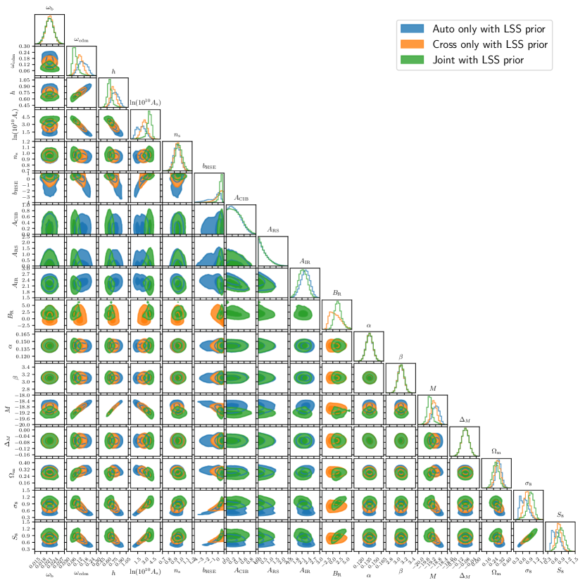
Figure 19: Confidence regions of cosmological parameters, hydrostatic bias parameter and all nuisance parameters inferred with three data sets (auto only, cross only, and joint) with the LSS prior. The inner (outer) contour corresponds to the $1\sigma$ ($2\sigma$) level. The diagonal panels show the marginalized likelihoods.

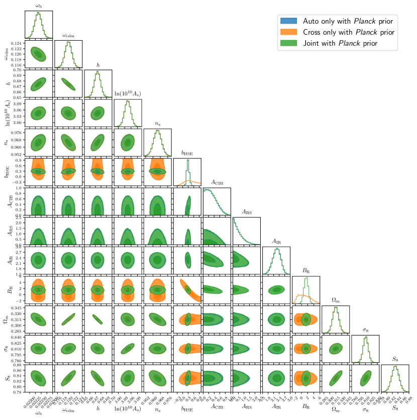
Figure 20: Confidence regions of cosmological parameters and hydrostatic bias parameter and all nuisance parameters inferred with three data sets (auto only, cross only, and joint) with the Planck prior. The inner (outer) contour corresponds to the $1\sigma$ ($2\sigma$) level. The diagonal panels show the marginalized likelihoods.

Table 7: Best-fit and median values estimated from parameter chains and marginalized constraints ($68\%$ C.L. and $95\%$ C.L.) on all parameters inferred from three data sets (auto only, cross only, and joint) with the LSS prior. The last three parameters ($\Omega_{\mathrm{m}}$, $\sigma_{8}$, and $S_{8}$) are derived parameters.

Auto only
Parameter	Range	Best-fit	Median	$68\%$ C.L.	$95\%$ C.L.
$\omega_{\mathrm{b}}$	—	$0.02226$	$0.02244$	$[0.02036,0.02451]$	$[0.01822,0.02653]$
$\omega_{\mathrm{cdm}}$	—	$0.1215$	$0.1664$	$[0.1232,0.2133]$	$[0.08282,0.2488]$
$h$	—	$0.6932$	$0.7906$	$[0.7072,0.8790]$	$[0.6239,0.9548]$
$\ln(10^{10}A_{\mathrm{s}})$	—	$3.140$	$2.244$	$[1.292,3.093]$	$[0.7963,3.889]$
$n_{\mathrm{s}}$	—	$0.9304$	$0.9470$	$[0.8914,1.004]$	$[0.8344,1.063]$
$b_{\mathrm{HSE}}$	$(-\infty,1]$	$0.3057$	$-0.2889$	$[-1.951,0.3169]$	$[-3.514,0.5868]$
$A_{\mathrm{CIB}}$	$[0,10]$	$0.1816$	$0.2768$	$[0.09240,0.5177]$	$[0.01450,0.7524]$
$A_{\mathrm{RS}}$	$[0,10]$	$0.2313$	$0.4124$	$[0.1087,0.9969]$	$[0.01561,1.780]$
$A_{\mathrm{IR}}$	$[0,10]$	$2.414$	$2.274$	$[2.035,2.496]$	$[1.800,2.696]$
$\alpha$	—	$0.1436$	$0.1412$	$[0.1346,0.1478]$	$[0.1280,0.1545]$
$\beta$	—	$3.085$	$3.105$	$[3.025,3.187]$	$[2.946,3.270]$
$M$	—	$-19.07$	$-18.78$	$[-19.02,-18.55]$	$[-19.31,-18.38]$
$\Delta_{M}$	—	$-0.07714$	$-0.07014$	$[-0.09346,-0.04660]$	$[-0.1171,-0.02307]$
$\Omega_{\mathrm{m}}$	—	$0.3005$	$0.3010$	$[0.2684,0.3339]$	$[0.2320,0.3683]$
$\sigma_{8}$	—	$0.8528$	$0.6687$	$[0.4930,0.8576]$	$[0.4228,1.056]$
$S_{8}$	—	$0.8536$	$0.6698$	$[0.5030,0.8395]$	$[0.4337,1.006]$

Cross only
Parameter	Range	Best-fit	Median	$68\%$ C.L.	$95\%$ C.L.
$\omega_{\mathrm{b}}$	—	$0.02255$	$0.02256$	$[0.02065,0.02447]$	$[0.01872,0.02642]$
$\omega_{\mathrm{cdm}}$	—	$0.1177$	$0.1380$	$[0.1077,0.1707]$	$[0.07441,0.2059]$
$h$	—	$0.6932$	$0.7411$	$[0.6821,0.8124]$	$[0.6139,0.8871]$
$\ln(10^{10}A_{\mathrm{s}})$	—	$3.201$	$2.816$	$[2.187,3.419]$	$[1.547,4.242]$
$n_{\mathrm{s}}$	—	$0.9444$	$0.9537$	$[0.9002,1.007]$	$[0.8445,1.063]$
$b_{\mathrm{HSE}}$	$(-\infty,1]$	$0.3339$	$0.3012$	$[-0.5595,0.7667]$	$[-2.261,0.9651]$
$B_{\mathrm{R}}$	$[-10,10]$	$1.679$	$0.7335$	$[-1.077,3.090]$	$[-2.020,5.333]$
$\alpha$	—	$0.1393$	$0.1414$	$[0.1348,0.1481]$	$[0.1282,0.1549]$
$\beta$	—	$3.087$	$3.107$	$[3.026,3.188]$	$[2.946,3.272]$
$M$	—	$-19.08$	$-18.92$	$[-19.11,-18.73]$	$[-19.35,-18.54]$
$\Delta_{M}$	—	$-0.06513$	$-0.06980$	$[-0.09318,-0.04654]$	$[-0.1167,-0.02346]$
$\Omega_{\mathrm{m}}$	—	$0.2932$	$0.2901$	$[0.2578,0.3225]$	$[0.2239,0.3559]$
$\sigma_{8}$	—	$0.8636$	$0.7929$	$[0.6584,0.9376]$	$[0.5352,1.156]$
$S_{8}$	—	$0.8538$	$0.7775$	$[0.6569,0.9015]$	$[0.5453,1.089]$

Joint
Parameter	Range	Best-fit	Median	$68\%$ C.L.	$95\%$ C.L.
$\omega_{\mathrm{b}}$	—	$0.02232$	$0.02247$	$[0.02044,0.02459]$	$[0.01834,0.02689]$
$\omega_{\mathrm{cdm}}$	—	$0.1225$	$0.09042$	$[0.07107,0.1208]$	$[0.05830,0.1834]$
$h$	—	$0.7080$	$0.6580$	$[0.6122,0.7121]$	$[0.5590,0.8294]$
$\ln(10^{10}A_{\mathrm{s}})$	—	$3.098$	$3.778$	$[3.297,4.169]$	$[1.827,4.468]$
$n_{\mathrm{s}}$	—	$0.9365$	$0.9740$	$[0.9192,1.033]$	$[0.8619,1.095]$
$b_{\mathrm{HSE}}$	$(-\infty,1]$	$0.2600$	$0.4755$	$[0.1548,0.6401]$	$[-0.9675,0.7336]$
$A_{\mathrm{CIB}}$	$[0,10]$	$0.1749$	$0.2973$	$[0.09437,0.5483]$	$[0.01332,0.7999]$
$A_{\mathrm{RS}}$	$[0,10]$	$0.3367$	$0.3847$	$[0.1019,0.9350]$	$[0.01393,1.623]$
$A_{\mathrm{IR}}$	$[0,10]$	$2.404$	$2.143$	$[1.926,2.367]$	$[1.707,2.568]$
$B_{\mathrm{R}}$	$[-10,10]$	$2.088$	$1.913$	$[0.7250,3.299]$	$[-0.3605,5.322]$
$\alpha$	—	$0.1433$	$0.1416$	$[0.1350,0.1484]$	$[0.1283,0.1551]$
$\beta$	—	$3.094$	$3.113$	$[3.031,3.194]$	$[2.951,3.277]$
$M$	—	$-19.02$	$-19.20$	$[-19.35,-19.02]$	$[-19.54,-18.68]$
$\Delta_{M}$	—	$-0.07639$	$-0.06996$	$[-0.09347,-0.04679]$	$[-0.1165,-0.02393]$
$\Omega_{\mathrm{m}}$	—	$0.2903$	$0.2680$	$[0.2327,0.3047]$	$[0.1996,0.3453]$
$\sigma_{8}$	—	$0.8445$	$0.9531$	$[0.8083,1.090]$	$[0.5673,1.218]$
$S_{8}$	—	$0.8307$	$0.8904$	$[0.7462,1.045]$	$[0.5680,1.185]$

Table 8: Best-fit and median values estimated from parameter chains and marginalized constraints ($68\%$ C.L. and $95\%$ C.L.) on all parameters inferred from three data sets (auto only, cross only, and joint) with the Planck prior. The last three parameters ($\Omega_{\mathrm{m}}$, $\sigma_{8}$, and $S_{8}$) are derived parameters.

Auto only
Parameter	Range	Best-fit	Median	$68\%$ C.L.	$95\%$ C.L.
$\omega_{\mathrm{b}}$	—	$0.02233$	$0.02237$	$[0.02222,0.02253]$	$[0.02206,0.02268]$
$\omega_{\mathrm{cdm}}$	—	$0.1201$	$0.1200$	$[0.1187,0.1212]$	$[0.1175,0.1224]$
$h$	—	$0.6729$	$0.6737$	$[0.6682,0.6793]$	$[0.6624,0.685]$
$\ln(10^{10}A_{\mathrm{s}})$	—	$3.044$	$3.044$	$[3.029,3.059]$	$[3.013,3.075]$
$n_{\mathrm{s}}$	—	$0.9655$	$0.9649$	$[0.9606,0.9691]$	$[0.9560,0.9737]$
$b_{\mathrm{HSE}}$	$(-\infty,1]$	$0.2367$	$0.2849$	$[0.2266,0.3548]$	$[0.1745,0.4241]$
$A_{\mathrm{CIB}}$	$[0,10]$	$0.1171$	$0.2601$	$[0.08309,0.4952]$	$[0.01245,0.7257]$
$A_{\mathrm{RS}}$	$[0,10]$	$0.06770$	$0.3941$	$[0.1039,0.9455]$	$[0.01391,1.717]$
$A_{\mathrm{IR}}$	$[0,10]$	$2.522$	$2.274$	$[2.051,2.479]$	$[1.820,2.663]$
$\Omega_{\mathrm{m}}$	—	$0.3160$	$0.3151$	$[0.3075,0.3227]$	$[0.3000,0.3308]$
$\sigma_{8}$	—	$0.8115$	$0.8106$	$[0.8043,0.8168]$	$[0.7976,0.8237]$
$S_{8}$	—	$0.8329$	$0.8307$	$[0.8173,0.844]$	$[0.8035,0.8582]$

Cross only
Parameter	Range	Best-fit	Median	$68\%$ C.L.	$95\%$ C.L.
$\omega_{\mathrm{b}}$	—	$0.02240$	$0.02238$	$[0.02222,0.02253]$	$[0.02204,0.02271]$
$\omega_{\mathrm{cdm}}$	—	$0.1201$	$0.1199$	$[0.1187,0.1212]$	$[0.1172,0.1227]$
$h$	—	$0.6734$	$0.6738$	$[0.6682,0.6795]$	$[0.6613,0.6863]$
$\ln(10^{10}A_{\mathrm{s}})$	—	$3.045$	$3.044$	$[3.029,3.059]$	$[3.010,3.076]$
$n_{\mathrm{s}}$	—	$0.9648$	$0.9650$	$[0.9606,0.9694]$	$[0.9554,0.9745]$
$b_{\mathrm{HSE}}$	$(-\infty,1]$	$0.3195$	$0.3932$	$[0.08367,0.7564]$	$[-0.1732,0.9653]$
$B_{\mathrm{R}}$	$[-10,10]$	$1.289$	$0.8204$	$[-1.040,3.115]$	$[-2.023,5.325]$
$\Omega_{\mathrm{m}}$	—	$0.3157$	$0.3148$	$[0.3072,0.3227]$	$[0.2986,0.3322]$
$\sigma_{8}$	—	$0.8115$	$0.8105$	$[0.8041,0.8169]$	$[0.7962,0.8245]$
$S_{8}$	—	$0.8325$	$0.8304$	$[0.8168,0.8441]$	$[0.8010,0.8601]$

Joint
Parameter	Range	Best-fit	Median	$68\%$ C.L.	$95\%$ C.L.
$\omega_{\mathrm{b}}$	—	$0.02235$	$0.02238$	$[0.02222,0.02254]$	$[0.02204,0.02274]$
$\omega_{\mathrm{cdm}}$	—	$0.1201$	$0.1199$	$[0.1187,0.1212]$	$[0.1170,0.1228]$
$h$	—	$0.6728$	$0.6738$	$[0.6680,0.6796]$	$[0.6609,0.6871]$
$\ln(10^{10}A_{\mathrm{s}})$	—	$3.044$	$3.044$	$[3.029,3.059]$	$[3.010,3.078]$
$n_{\mathrm{s}}$	—	$0.9644$	$0.9649$	$[0.9604,0.9694]$	$[0.9546,0.9746]$
$b_{\mathrm{HSE}}$	$(-\infty,1]$	$0.2692$	$0.2857$	$[0.2251,0.3578]$	$[0.1695,0.4323]$
$A_{\mathrm{CIB}}$	$[0,10]$	$0.2876$	$0.2691$	$[0.08802,0.5089]$	$[0.01381,0.7486]$
$A_{\mathrm{RS}}$	$[0,10]$	$0.04537$	$0.4048$	$[0.1057,0.9772]$	$[0.01403,1.780]$
$A_{\mathrm{IR}}$	$[0,10]$	$2.425$	$2.266$	$[2.040,2.474]$	$[1.812,2.663]$
$B_{\mathrm{R}}$	$[-10,10]$	$1.498$	$1.522$	$[0.8353,2.180]$	$[0.1187,2.824]$
$\Omega_{\mathrm{m}}$	—	$0.3161$	$0.3149$	$[0.3071,0.3228]$	$[0.2976,0.3326]$
$\sigma_{8}$	—	$0.8111$	$0.8105$	$[0.8040,0.8170]$	$[0.7955,0.8250]$
$S_{8}$	—	$0.8326$	$0.8304$	$[0.8166,0.8443]$	$[0.7989,0.8612]$

References

- Aihara et al. (2018a) Aihara H., et al., 2018a, PASJ, 70, S4
- Aihara et al. (2018b) Aihara H., et al., 2018b, PASJ, 70, S8
- Alam et al. (2017) Alam S., et al., 2017, MNRAS, 470, 2617
- Arnaud et al. (2010) Arnaud M., Pratt G. W., Piffaretti R., Böhringer H., Croston J. H., Pointecouteau E., 2010, A&A, 517, A92
- Audren et al. (2013) Audren B., Lesgourgues J., Benabed K., Prunet S., 2013, J. Cosmology Astropart. Phys., 2013, 001
- Battaglia et al. (2012a) Battaglia N., Bond J. R., Pfrommer C., Sievers J. L., 2012a, ApJ, 758, 74
- Battaglia et al. (2012b) Battaglia N., Bond J. R., Pfrommer C., Sievers J. L., 2012b, ApJ, 758, 75
- Battaglia et al. (2015) Battaglia N., Hill J. C., Murray N., 2015, ApJ, 812, 154
- Battaglia et al. (2016) Battaglia N., et al., 2016, J. Cosmology Astropart. Phys., 2016, 013
- Betoule et al. (2014) Betoule M., et al., 2014, A&A, 568, A22
- Biffi et al. (2016) Biffi V., et al., 2016, ApJ, 827, 112
- Bleem et al. (2012) Bleem L., et al., 2012, Journal of Low Temperature Physics, 167, 859
- Bocquet et al. (2016) Bocquet S., Saro A., Dolag K., Mohr J. J., 2016, MNRAS, 456, 2361
- Bode et al. (2009) Bode P., Ostriker J. P., Vikhlinin A., 2009, ApJ, 700, 989
- Bolliet et al. (2018) Bolliet B., Comis B., Komatsu E., Macías-Pérez J. F., 2018, MNRAS, 477, 4957
- Bosch et al. (2018) Bosch J., et al., 2018, PASJ, 70, S5
- Brinckmann & Lesgourgues (2018) Brinckmann T., Lesgourgues J., 2018, arXiv e-prints, p. arXiv:1804.07261
- Bryan & Norman (1998) Bryan G. L., Norman M. L., 1998, ApJ, 495, 80
- Chluba et al. (2012) Chluba J., Nagai D., Sazonov S., Nelson K., 2012, MNRAS, 426, 510
- Dolag et al. (2016) Dolag K., Komatsu E., Sunyaev R., 2016, MNRAS, 463, 1797
- Flender et al. (2017) Flender S., Nagai D., McDonald M., 2017, ApJ, 837, 124
- Górski et al. (2005) Górski K. M., Hivon E., Banday A. J., Wand elt B. D., Hansen F. K., Reinecke M., Bartelmann M., 2005, ApJ, 622, 759
- Henson et al. (2017) Henson M. A., Barnes D. J., Kay S. T., McCarthy I. G., Schaye J., 2017, MNRAS, 465, 3361
- Hikage et al. (2019) Hikage C., et al., 2019, PASJ, 71, 43
- Hinshaw et al. (2013) Hinshaw G., et al., 2013, ApJS, 208, 19
- Hirata & Seljak (2003) Hirata C., Seljak U., 2003, MNRAS, 343, 459
- Hivon et al. (2002) Hivon E., Górski K. M., Netterfield C. B., Crill B. P., Prunet S., Hansen F., 2002, ApJ, 567, 2
- Hoekstra et al. (2015) Hoekstra H., Herbonnet R., Muzzin A., Babul A., Mahdavi A., Viola M., Cacciato M., 2015, MNRAS, 449, 685
- Hojjati et al. (2017) Hojjati A., et al., 2017, MNRAS, 471, 1565
- Hurier et al. (2013) Hurier G., Macías-Pérez J. F., Hildebrandt S., 2013, A&A, 558, A118
- Ilbert et al. (2009) Ilbert O., et al., 2009, ApJ, 690, 1236
- Itoh et al. (1998) Itoh N., Kohyama Y., Nozawa S., 1998, ApJ, 502, 7
- Kaiser & Squires (1993) Kaiser N., Squires G., 1993, ApJ, 404, 441
- Klypin et al. (2016) Klypin A., Yepes G., Gottlöber S., Prada F., Heß S., 2016, MNRAS, 457, 4340
- Komatsu & Kitayama (1999) Komatsu E., Kitayama T., 1999, ApJ, 526, L1
- Komatsu & Seljak (2001) Komatsu E., Seljak U., 2001, MNRAS, 327, 1353
- Komatsu & Seljak (2002) Komatsu E., Seljak U., 2002, MNRAS, 336, 1256
- Kuijken et al. (2015) Kuijken K., et al., 2015, MNRAS, 454, 3500
- Laigle et al. (2016) Laigle C., et al., 2016, ApJS, 224, 24
- Lau et al. (2009) Lau E. T., Kravtsov A. V., Nagai D., 2009, ApJ, 705, 1129
- Lau et al. (2013) Lau E. T., Nagai D., Nelson K., 2013, ApJ, 777, 151
- Lewis et al. (2000) Lewis A., Challinor A., Lasenby A., 2000, ApJ, 538, 473
- Ma et al. (2015) Ma Y.-Z., Van Waerbeke L., Hinshaw G., Hojjati A., Scott D., Zuntz J., 2015, J. Cosmology Astropart. Phys., 2015, 046
- Makino & Suto (1993) Makino N., Suto Y., 1993, ApJ, 405, 1
- Makino et al. (1998) Makino N., Sasaki S., Suto Y., 1998, ApJ, 497, 555
- Makiya et al. (2018) Makiya R., Ando S., Komatsu E., 2018, MNRAS, 480, 3928
- Makiya et al. (2019) Makiya R., Hikage C., Komatsu E., 2019, arXiv e-prints, p. arXiv:1907.07870
- Mandelbaum et al. (2018a) Mandelbaum R., et al., 2018a, PASJ, 70, S25
- Mandelbaum et al. (2018b) Mandelbaum R., et al., 2018b, MNRAS, 481, 3170
- McCarthy et al. (2014) McCarthy I. G., Le Brun A. M. C., Schaye J., Holder G. P., 2014, MNRAS, 440, 3645
- Medezinski et al. (2018) Medezinski E., et al., 2018, PASJ, 70, S28
- Miyatake et al. (2019) Miyatake H., et al., 2019, ApJ, 875, 63
- Miyazaki et al. (2015) Miyazaki S., et al., 2015, ApJ, 807, 22
- Miyazaki et al. (2018) Miyazaki S., et al., 2018, PASJ, 70, S1
- Nagai (2006) Nagai D., 2006, ApJ, 650, 538
- Nagai et al. (2007a) Nagai D., Vikhlinin A., Kravtsov A. V., 2007a, ApJ, 655, 98
- Nagai et al. (2007b) Nagai D., Kravtsov A. V., Vikhlinin A., 2007b, ApJ, 668, 1
- Navarro et al. (1996) Navarro J. F., Frenk C. S., White S. D. M., 1996, ApJ, 462, 563
- Navarro et al. (1997) Navarro J. F., Frenk C. S., White S. D. M., 1997, ApJ, 490, 493
- Nelson et al. (2014a) Nelson K., Lau E. T., Nagai D., Rudd D. H., Yu L., 2014a, ApJ, 782, 107
- Nelson et al. (2014b) Nelson K., Lau E. T., Nagai D., 2014b, ApJ, 792, 25
- Nozawa et al. (1998) Nozawa S., Itoh N., Kohyama Y., 1998, ApJ, 508, 17
- Oguri et al. (2018) Oguri M., et al., 2018, PASJ, 70, S26
- Osato et al. (2018) Osato K., Flender S., Nagai D., Shirasaki M., Yoshida N., 2018, MNRAS, 475, 532
- Pedregosa et al. (2011) Pedregosa F., et al., 2011, Journal of Machine Learning Research, 12, 2825
- Penna-Lima et al. (2017) Penna-Lima M., Bartlett J. G., Rozo E., Melin J. B., Merten J., Evrard A. E., Postman M., Rykoff E., 2017, A&A, 604, A89
- Planck Collaboration et al. (2013) Planck Collaboration et al., 2013, A&A, 550, A131
- Planck Collaboration et al. (2016a) Planck Collaboration et al., 2016a, A&A, 594, A22
- Planck Collaboration et al. (2016b) Planck Collaboration et al., 2016b, A&A, 594, A27
- Planck Collaboration et al. (2018a) Planck Collaboration et al., 2018a, arXiv e-prints, p. arXiv:1807.06209
- Planck Collaboration et al. (2018b) Planck Collaboration et al., 2018b, arXiv e-prints, p. arXiv:1807.06210
- Pratt et al. (2019) Pratt G. W., Arnaud M., Biviano A., Eckert D., Ettori S., Nagai D., Okabe N., Reiprich T. H., 2019, Space Sci. Rev., 215, 25
- Rasia et al. (2014) Rasia E., et al., 2014, ApJ, 791, 96
- Remazeilles et al. (2011) Remazeilles M., Delabrouille J., Cardoso J.-F., 2011, MNRAS, 410, 2481
- Scoccimarro et al. (2001) Scoccimarro R., Sheth R. K., Hui L., Jain B., 2001, ApJ, 546, 20
- Sereno et al. (2017) Sereno M., Covone G., Izzo L., Ettori S., Coupon J., Lieu M., 2017, MNRAS, 472, 1946
- Shaw et al. (2010) Shaw L. D., Nagai D., Bhattacharya S., Lau E. T., 2010, ApJ, 725, 1452
- Shi et al. (2015) Shi X., Komatsu E., Nelson K., Nagai D., 2015, MNRAS, 448, 1020
- Shi et al. (2016) Shi X., Komatsu E., Nagai D., Lau E. T., 2016, MNRAS, 455, 2936
- Shirasaki (2019) Shirasaki M., 2019, MNRAS, 483, 342
- Shirasaki et al. (2016) Shirasaki M., Nagai D., Lau E. T., 2016, MNRAS, 460, 3913
- Shirasaki et al. (2019) Shirasaki M., Hamana T., Takada M., Takahashi R., Miyatake H., 2019, MNRAS, 486, 52
- Smith et al. (2016) Smith G. P., et al., 2016, MNRAS, 456, L74
- Sunyaev & Zel’dovich (1972) Sunyaev R. A., Zel’dovich Y. B., 1972, Comments on Astrophysics and Space Physics, 4, 173
- Sunyaev & Zel’dovich (1980) Sunyaev R. A., Zel’dovich Y. B., 1980, MNRAS, 190, 413
- Suto et al. (2013) Suto D., Kawahara H., Kitayama T., Sasaki S., Suto Y., Cen R., 2013, ApJ, 767, 79
- Swetz et al. (2011) Swetz D. S., et al., 2011, ApJS, 194, 41
- Takahashi et al. (2017) Takahashi R., Hamana T., Shirasaki M., Namikawa T., Nishimichi T., Osato K., Shiroyama K., 2017, ApJ, 850, 24
- Tanaka et al. (2018) Tanaka M., et al., 2018, PASJ, 70, S9
- Tinker et al. (2010) Tinker J. L., Robertson B. E., Kravtsov A. V., Klypin A., Warren M. S., Yepes G., Gottlöber S., 2010, ApJ, 724, 878
- Van Waerbeke et al. (2014) Van Waerbeke L., Hinshaw G., Murray N., 2014, Phys. Rev. D, 89, 023508
- Vazza et al. (2018) Vazza F., Angelinelli M., Jones T. W., Eckert D., Brüggen M., Brunetti G., Gheller C., 2018, MNRAS, 481, L120
- Zuntz et al. (2018) Zuntz J., et al., 2018, MNRAS, 481, 1149
- von der Linden et al. (2014) von der Linden A., et al., 2014, MNRAS, 443, 1973