Hidden Unit Specialization in Layered Neural Networks: ReLU vs. Sigmoidal Activation

Abstract

By applying concepts from the statistical physics of learning, we study layered neural networks of rectified linear units (ReLU). The comparison with conventional, sigmoidal activation functions is in the center of interest. We compute typical learning curves for large shallow networks with $K$ hidden units in matching student teacher scenarios. The systems undergo phase transitions, i.e. sudden changes of the generalization performance via the process of hidden unit specialization at critical sizes of the training set. Surprisingly, our results show that the training behavior of ReLU networks is qualitatively different from that of networks with sigmoidal activations. In networks with $K\geq 3$ sigmoidal hidden units, the transition is discontinuous: Specialized network configurations co-exist and compete with states of poor performance even for very large training sets. On the contrary, the use of ReLU activations results in continuous transitions for all $K.$ For large enough training sets, two competing, differently specialized states display similar generalization abilities, which coincide exactly for large hidden layers in the limit $K\to\infty.$ Our findings are also confirmed in Monte Carlo simulations of the training processes.

1 Introduction

The re-gained interest in artificial neural networks [1, 2, 3, 4, 5] is largely due to the successful application of so-called Deep Learning in a number of practical contexts, see e.g. [6, 7, 8] for reviews and further references.

The successful training of powerful, multi-layered deep networks has become feasible for a number of reasons including the automated acquisition of large amounts of training data in various domains, the use of modified and optimized architectures, e.g. convolutional networks for image processing, and the ever-increasing availability of computational power needed for the implementation of efficient training.

One particularly important modification of earlier models is the use of alternative activation functions [6, 9, 10]. Arguably, so-called rectified linear units (ReLU) constitute the most popular choice in Deep Neural Networks [6, 9, 10, 11, 12, 13]. Compared to more traditional activation functions, the simple ReLU and recently suggested modifications warrant computational ease and appear to speed up the training, see for instance [11, 14, 15]. The one-sided ReLU function is found to yield sparse activity in large networks, a feature which is frequently perceived as favorable and biologically plausible [6, 12, 16]. In addition, the problem of vanishing gradients, which arises when applying the chain rule in layered networks of sigmoidal units, is avoided [6]. Moreover, networks of rectified linear units have displayed favorable generalization behavior in several practical applications and benchmark tests, e.g.  [9, 10, 11, 12, 13].

The aim of this work is to contribute to a better theoretical understanding of how the use of ReLU activations influences and potentially improves the training behavior of layered neural networks. We focus on the comparison with traditional sigmoidal functions and analyse non-trivial model situations. To this end, we employ approaches from the statistical physics of learning, which have been applied earlier with great success in the context of neural networks and machine learning in general [1, 3, 17, 18, 19, 20, 21]. The statistical physics approach complements other theoretical frameworks in that it studies the typical behavior of large learning systems in model scenarios. As an important example, learning curves have been computed in a variety of settings, including on-line and off-line supervised training of feedforward neural networks, see for instance [3, 17, 18, 19, 20, 21, 22, 23, 24, 25, 26, 27] and references therein. A topic of particular interest for this work is the analysis of phase transitions in learning processes, i.e.  sudden changes of the expected performance with the training set size or other control parameters, see [19, 20, 27, 28, 29, 30, 31, 32] for examples and further references.

Currently, the statistical physics of learning is being revisited extensively in order to investigate relevant phenomena in deep neural networks and other learning paradigms, see [33, 34, 35, 36, 37, 38, 39, 40] for recent examples and further references.

In this work, we systematically study the training of layered networks in so-called student teacher settings, see e.g. [3, 17, 18, 20]. We consider idealized, yet non-trivial scenarios of matching student and teacher complexity. Our findings demonstrate that ReLU networks display training and generalization behavior which differs significantly from their counterparts composed of sigmoidal units. Both network types display sudden changes of their performance with the number of available examples. In statistical physics terminology, the systems undergo phase transitions at a critical training set size. The underlying process of hidden unit specialization and the existence of saddle points in the objective function have recently attracted attention also in the context of Deep Learning [34, 41, 42].

Before analysing ReLU networks, we confirm earlier theoretical results which indicate that the transition for large networks of sigmoidal units is discontinuous (first order): For small training sets, a poorly generalizing state is observed, in which all hidden units approximate the target to some extent and essentially perform the same task. At a critical size of the training set, a favorable configuration with specialized hidden units appears. However, a poorly performing state remains metastable and the specialization required for successful learning can delay the training process significantly [28, 29, 30, 31].

In contrast we find that, surprisingly, the corresponding phase transition in ReLU networks is always continuous (second order). At the transition, the unspecialized state is replaced by two competing configurations with very similar generalization ability. In large networks, their performance is nearly identical and it coincides exactly in the limit $K\to\infty.$

In the next section we detail the considered models and outline the theoretical approach. In Sec. 3 our results are presented and discussed. In addition, results of supporting Monte Carlo simulations are presented. We conclude with a summary and outlook on future extensions of this work.

2 Model and Analysis

Here we introduce the modelling framework, i.e. the considered student teacher scenarios. Moreover, we outline their analysis by means of statistical physics methods and discuss the simplifying assumption of training at high (formal) temperatures.

2.1 Network architecture and activation functions

We consider feed-forward neural networks where $N$ input nodes represent feature vectors $\boldsymbol{\xi}\in\mathbb{R}^{N}.$ A single layer of $K$ hidden units is connected to the input through adaptive weights $\underline{W}=\left\{\mathbf{w}_{k}\in\mathbb{R}^{N}\right\}_{k=1}^{K}.$ The total real-valued output reads

$$\sigma(\boldsymbol{\xi})=\frac{1}{\sqrt{K}}\sum_{k=1}^{K}\,g\left(x_{k}\right)\mbox{~{}~{}with~{}~{}}x_{k}=\frac{1}{\sqrt{N}}\mathbf{w}_{k}\cdot\boldsymbol{\xi}.$$ (1)

The quantity $x_{k}$ is referred to as the local potential of the hidden unit. The resulting activation is specified by the function $g(x)$ and hidden to output weights are fixed to $1/\sqrt{K}$. Figure 1 (a) illustrates the network architecture.

This type of network has been termed the Soft Committee Machine (SCM) in the literature due to its vague similarity to the committee machine for binary classification, e.g.  [3, 18, 20, 27, 39, 43, 44]. There, the discrete output is determined by the majority of threshold units in the hidden layer, while the SCM is suitable for regression tasks.

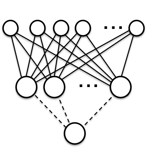
Figure 1: (a) Illustration of the network architecture with an $N$-dim. input layer, a set of adaptive weight vectors $\mathbf{w}_{k}\mbox{~{}with~{}}k\!=\!1,\!\ldots\!,K$ (represented by solid lines) and total output $\sigma$ given by the sum of hidden unit activations with fixed weights (dashed lines). (b) The considered activation functions: the sigmoidal $g(x)=\left(1+\mbox{erf}[x/\sqrt{2}]\right)$ (solid line) and the ReLU activation $g(x)=\mbox{\rm max}\{0,x\}$ (dashed line).

We will consider two popular types of transfer functions:

• Sigmoidal activation
  Frequently, S-shaped transfer functions $g(x)$ have been employed, which increase monotonically from zero at large negative arguments and saturate at a finite maximum for $x\to\infty$. Popular examples are based on $\tanh(x)$ or the sigmoid $(1+e^{-x})^{-1}$, often with an additional threshold $\theta$ as in $g(x-\theta),$ or a steepness parameter controlling the magnitude of the derivative $g^{\prime}.$ We study in particular

  $$\textstyle g(x)=\left(1+\mbox{erf}\left[\frac{x}{\sqrt{2}}\right]\right)=2\int\limits_{-\infty}^{x}dz\frac{e^{-z^{2}/2}}{\sqrt{2\pi}}$$ (2)

  with $0\leq g(x)\leq 2,$ which is displayed in Fig. 1 (b). The relation to an integrated Gaussian facilitates significant mathematical ease, which has been exploited in numerous studies of machine learning models, e.g. [22, 23, 24]. Here, the function (2) serves as a generic example of a sigmoidal and its specific form is not expected to influence our findings crucially. As we argue below, the choice of limiting values $0$ and $2$ for small and large arguments, respectively, is also arbitrary and irrelevant for the qualitative results of our analyses.
  

• Rectified Linear Unit (ReLU) activation
  This particularly simple, piece-wise linear transfer function has attracted considerable attention in the context of multi-layered neural networks:

  $$g(x)=\,\mbox{max}\left\{0,x\right\}=\left\{\begin{array}[]{cc}0&\mbox{~{}~{}for~{}}x\leq 0\\ x&\mbox{~{}~{}for~{}}x>0\\ \end{array}\right.$$ (3)

  which is illustrated in Fig. 1 (b). In contrast to sigmoidal activations, the response of the unit is unbounded for $x\to\infty$.

  The function (3) is obviously not differentiable in $x=0$. Here, we can ignore this mathematical subtlety and remark that it is considered irrelevant in practice [6]. Note also that our theoretical investigation in Sec. 2 does not relate to a particular realization of gradient-based training.

It is important to realize that replacing the above functions by $g(x)=\gamma\,\left(1+\mbox{erf}[x/\sqrt{2}]\right)$ in (a) or by $g(x)=\max\{0,\gamma\,x\}=\gamma\,\max\{0,x\}$ in (b), where $\gamma>0$ is an arbitrary factor, would be equivalent to setting the hidden unit weights to $\gamma/\sqrt{K}$ in Eq. (1). Alternatively, we could incorporate the factor $\gamma$ in the effective temperature parameter $\alpha$ of the theoretical analysis in Sec. 2.4. Apart from this trivial re-scaling, our results would not be affected qualitatively.

2.2 Student and teacher scenario

We investigate the training and generalization behavior of the layered networks introduced above in a setup that models the learning of a regression scheme from example data. Assume that a given training set

$$\textstyle\mathbb{D}=\left\{\boldsymbol{\xi}^{\mu},\tau^{\mu}\right\}_{\mu=1}^{P}$$ (4)

comprises $P$ input output pairs which reflect the target task. In order to facilitate successful learning, $P$ should be proportional to the number of adaptive weights in the trained system. In our specific model scenario the labels $\tau^{\mu}=\tau(\boldsymbol{\xi}^{\mu})$ are thought to be provided by a teacher SCM, representing the target input output relation

$$\tau(\boldsymbol{\xi})\textstyle=\frac{1}{\sqrt{M}}\sum_{m=1}^{M}\,g\left(x_{m}^{*}\right)\mbox{~{}~{}with~{}~{}}x_{m}^{*}=\frac{1}{\sqrt{N}}\mathbf{w}_{m}^{*}\cdot\boldsymbol{\xi}.$$ (5)

The response is specified in terms of the set of teacher weight vectors $\underline{W}^{*}=\left\{\mathbf{w}_{m}^{*}\right\}_{m=1}^{M}$ and defines the correct target output for every possible feature vector $\boldsymbol{\xi}$. For simplicity, we focus on settings with orthonormal teacher weight vectors and restrict the adaptive student configuration to normalized weights:

$$\mathbf{w}_{m}^{*}\cdot\mathbf{w}_{n}^{*}/N=\delta_{mn}\mbox{~{}~{}and~{}~{}}|\mathbf{w}_{j}|^{2}=N\mbox{~{}~{}with the Kronecker-Delta~{}}\delta_{mn}.$$ (6)

Throughout the following, the evaluation of the student network will be based on a simple quadratic error measure that compares student output and target value. Accordingly, the selection of student weights $\underline{W}$ in the training process is guided by a cost function which is given by the corresponding sum over all available data in $\mathbb{D}$:

$$E=\sum_{\mu=1}^{P}\epsilon(\boldsymbol{\xi}^{\mu})\mbox{~{}~{}with~{}~{}}\epsilon(\boldsymbol{\xi})=\frac{1}{2}\bigg{(}\sigma(\boldsymbol{\xi})-\tau(\boldsymbol{\xi})\bigg{)}^{2}.$$ (7)

By choosing the parameters $K$ and $M$, a variety of situations can be modelled. This includes the learning of unrealizable rules ($K<M$) and training of over-sophisticated students with $K>M$. Here, we restrict ourselves to the idealized, yet non-trivial case of perfectly matching student and teacher complexity, i.e. $K=M$, which makes it possible to achieve $\epsilon(\boldsymbol{\xi})=0$ for all input vectors.

2.3 Generalization error and order parameters

Throughout the following we consider feature vectors $\boldsymbol{\xi}^{\mu}$ in the training set with uncorrelated i.i.d. random components of zero mean and unit variance. Likewise, arbitrary input vectors $\boldsymbol{\xi}\not\in\mathbb{D}$ are assumed to follow the same statistics:

$$\left\langle\xi_{j}^{\mu}\right\rangle=0,\,\left\langle\xi_{j}^{\mu}\xi_{k}^{\nu}\right\rangle=\delta_{j,k}\delta_{\mu,\nu},\,\left\langle\xi_{j}\right\rangle=0\mbox{~{}and~{}}\left\langle\xi_{j}\xi_{k}\right\rangle=\delta_{j,k}.$$

As a consequence of this assumption, the Central Limit Theorem applies to the local potentials $x_{j}^{(*)}=\mathbf{w}_{j}^{(*)}\cdot\boldsymbol{\xi}/\sqrt{N}$ which become correlated Gaussian random variables of order ${\cal O}(1)$. It is straightforward to work out the averages $\left\langle\ldots\right\rangle$ and (co-)variances:

$$\left\langle x_{k}\right\rangle=\left\langle x_{k}^{*}\right\rangle=0,\mbox{~{}}\left\langle x_{j}x_{k}\right\rangle=\,\mathbf{w}_{j}\cdot\mathbf{w}_{k}/N\,\equiv\,Q_{jk},$$ (8)

$$\left\langle x_{j}^{*}x_{k}^{*}\right\rangle=\mathbf{w}^{*}_{j}\cdot\mathbf{w}_{k}^{*}/N=\delta_{jk}\mbox{~{}and~{}}\left\langle x_{j}x_{k}^{*}\right\rangle=\mathbf{w}_{j}\cdot\mathbf{w}_{k}^{*}/N\equiv\,R_{jk},$$

which fully specify the joint density $P\left(\left\{x_{i},x_{i}^{*}\right\}\right)$. The order parameters $R_{ij}$ and $Q_{ij}$ for $(i,j=1,2,\ldots K)$ serve as macroscopic characteristics of the student configuration. The norms $Q_{ii}=1$ are fixed according to Eq. (6), while the symmetric $Q_{ij}=Q_{ji}$ quantify the $K(K-1)/2$ pairwise alignments of student weight vectors. The similarity of the student weights to their counterparts in the teacher network are measured in terms of the $K^{2}$ quantities $R_{ij}$. Due to the assumed normalizations, the relations $-\!1\!\leq\!Q_{ij},R_{ij}\!\leq\!1$ are obviously satisfied.

Now we can work out the generalization error, i.e. the expected deviation of student and teacher output for a random input vector, given specific weight configurations $\underline{W}$ and $\underline{W}^{*}$. Note that SCM with $g(x)=\mbox{erf}[x/\sqrt{2}]$ have been treated in [23, 24] for general $K,M.$ Here, we resort to the special case of matching network sizes, $K=M,$ with

$$\epsilon_{g}\, = \,\frac{1}{2K}\left\langle\bigg{(}\sum_{i=1}^{K}g(x_{i})-\sum_{j=1}^{K}g(x_{j}^{*})\bigg{)}^{2}\right\rangle.$$ (9)

We note here that matching additive constants in the student and teacher activations would leave $\epsilon_{g}$ unaltered. As detailed in the Appendix, all averages in Eq. (9) can be computed analytically for both choices of the activation function $g(x)$ in student and teacher network. Eventually, the generalization error is expressed in terms of very few macroscopic order parameters, instead of explicitly taking into account $KN$ individual weights. The concept is characteristic for the statistical physics approach to systems with many degrees of freedom. In the following, we restrict the analysis to student configurations which are site-symmetric with respect to the hidden units:

$$R_{ij}=\left\{\begin{array}[]{ll}R&\mbox{for~{}}i=j\\ S&\mbox{otherwise,}\\ \end{array}\right.\mbox{~{}~{}~{}~{}}Q_{ij}=\left\{\begin{array}[]{ll}1&\mbox{for~{}}i=j\\ C&\mbox{otherwise.}\\ \end{array}\right.$$ (10)

Obviously, the system is invariant under permutations, so we can restrict ourselves to one specific case with matching indices $i=j$ in Eq. (10). While this assumption reflects the symmetries of the student teacher scenario, it allows for the specialization of hidden units: For $R=S$ all student units display the same overlap with all teacher units. In specialized configurations with $R\neq S$, however, each student weight vector has achieved a distinct overlap with exactly one of the teacher units. Our analysis shows that states with both positive ($R>S$) and negative specialization ($R<S$) can play a significant role in the training process. Under the above assumption of site-symmetry (10) and applying the normalization (6), the generalization error (9), see also Eqs. (26,29), becomes

a) for $g(x)=\left(1\!+\!\mbox{erf}\big{[}{x/\sqrt{2}}\big{]}\right)$ in student and teacher [23]:

$$\textstyle\epsilon_{g}\!=\!\frac{1}{K}\left\{\frac{1}{3}\!+\!\frac{K\!-\!1}{\pi}\left[\sin^{-1}\left(\frac{C}{2}\right)\!-\!2\sin^{-1}\left(\frac{S}{2}\right)\right]\!-\!\frac{2}{\pi}\sin^{-1}\left(\frac{R}{2}\right)\right\},$$ (11)

b) for ReLU $g(x)=\mbox{max}\{0,x\}$ [45]:

$$\epsilon_{g} = \textstyle\frac{1}{2K}\left\{K\!+\!\frac{(K^{2}\!-\!K)}{2\pi}\!-\!2K\!\left(\frac{R}{4}+\frac{\sqrt{1-R^{2}}}{2\pi}+\frac{R\sin^{-1}(R)}{2\pi}\right)\right.$$

$$+ \!\!\!\!\textstyle(K^{2}\!-\!K)\left(\frac{C}{4}\!+\!\frac{\sqrt{1-C^{2}}}{2\pi}\!+\!\frac{C\sin^{-1}(C)}{2\pi}\right)-\textstyle\!\!\left.2(K^{2}\!-\!K)\left(\frac{S}{4}\!+\!\frac{\sqrt{1-S^{2}}}{2\pi}\!+\!\frac{S\sin^{-1}(S)}{2\pi}\right)\right\}.$$

In both settings, perfect agreement of student and teacher with $\epsilon_{g}=0$ is achieved for $C\!=\!S\!=\!0$ and $R\!=\!1.$ The scaling of outputs with hidden to output weights $1/\sqrt{K}$ in Eq. (1) results in a generalization error which is not explicitly $K$-dependent for uncorrelated random students: A configuration with $R=C=S=0$ yields $\epsilon_{g}=1/3$ in the case of sigmoidal activations (a), whereas $\epsilon_{g}=\frac{1}{2}-\frac{1}{2\pi}\approx 0.341$ for ReLU student and teacher.

2.4 Thermal equilibrium and the high-temperature limit

In order to analyse the expected outcome of training from a set of examples $\mathbb{D}$, we follow the well-established statistical physics approach and analyse an ensemble of networks in a formal thermal equilibrium situation. In this framework, the cost function $E$ is interpreted as the energy of the system and the density of observed network states is given by the so-called Gibbs-Boltzmann density

$$\textstyle\left.{\exp[-\beta E]}\right/{Z}\mbox{~{}~{}~{}with~{}~{}}Z=\int d\mu(\underline{W})\exp[-\beta E],$$ (13)

where the measure $d\mu(\underline{W})$ incorporates potential restrictions of the integration over all possible configurations of $\underline{W}=\left\{\mathbf{w}_{i}\right\}_{i=1}^{K},$ for instance the normalization $\mathbf{w}_{k}^{2}=N$ for all $k$. This equilibrium density could result from a Langevin type of training dynamics

$$\left.{\partial\underline{W}}\right/{\partial t}\,=\,-\nabla_{W}\,E(\underline{W})\,+\underline{\eta},$$

where $\nabla_{W}$ denotes the gradient with respect to all $KN$ degrees of freedom in the student network. Here, the minimization of $E$ is performed in the presence of a $\delta$-correlated, zero mean noise term $\underline{\eta}(t)\in\mathbb{R}^{KN}$ with

$$\left\langle\eta_{i}(t)\right\rangle=0\mbox{~{}~{}and~{}~{}}\left\langle\eta_{i}(t)\eta_{j}\right(t^{\prime})\rangle=2\beta\delta_{ij}\delta(t-t^{\prime}),$$

where $\delta(\ldots)$ denotes the Dirac delta-function. The parameter $\beta=1/T$ controls the strength of the thermal noise in the gradient-based minimization of $E$. According to the, by now, standard statistical physics approach to off-line learning [1, 3, 18, 17] typical properties of the system are governed by the so-called quenched free energy

$$f=-\left.{1}\right/{N}\,\left\langle\,\ln Z\right\rangle_{\mathbb{D}}/\beta$$ (14)

where $\left\langle\ldots\right\rangle_{\mathbb{D}}$ denotes the average over the random realization of the training set. In general, the evaluation of the quenched average $\left\langle\ln Z\right\rangle_{\mathbb{D}}$ is technically involved and requires, for instance, the application of the replica trick [1, 3, 18]. Here, we resort to the simplifying limit of training at high temperature $\ T\to\infty,\beta\to 0$, which has proven useful in the qualitative investigation of various learning scenarios [17]. In the limit $\beta\to 0$ the so-called annealed approximation [17, 18, 3] $\left\langle\ln Z\right\rangle_{\mathbb{D}}\approx\ln\left\langle Z\right\rangle_{\mathbb{D}}$ becomes exact. Moreover, we have

$$\textstyle\left\langle Z\right\rangle_{\mathbb{D}}=\left\langle\int d\mu(\underline{W})e^{-\beta E}\right\rangle_{\mathbb{D}}\approx\int d\mu(\underline{W})e^{-\beta\left\langle E\right\rangle_{I\!\!D}}.$$ (15)

Here, $P$ is the number of statistically independent examples in $\mathbb{D}$ and $\left\langle E\right\rangle_{\mathbb{D}}=P\left\langle\epsilon(\boldsymbol{\xi})\right\rangle_{\xi}=P\epsilon_{g}$. As the exponent grows linearly with $P\propto N$, the integral is dominated by the maximum of the integrand. By means of a saddle-point integration for $N\to\infty$ we obtain

$$-\frac{1}{N}\ln\left\langle Z\right\rangle_{\mathbb{D}}\,=\beta f(\{R_{ij},Q_{ij}\})\approx\frac{\beta P}{N}\epsilon_{g}-s.$$ (16)

Here, the right hand side has to be minimized with respect to the arguments, i.e. the order parameters $\left\{R_{ij},Q_{ij}\right\}.$ In Eq. (16) we have introduced the entropy term

$$\textstyle s\!=\!\frac{1}{N}\!\ln\!\int\!d\mu(\underline{W})\!\prod_{i,j}\!\left[\delta(NR_{ij}\!-\!\mathbf{w}_{i}\cdot\mathbf{w}^{*}_{j})\delta(NQ_{ij}\!-\!\mathbf{w}_{i}\!\cdot\!\mathbf{w}_{j})\right].$$ (17)

The quantity $e^{N}s$ corresponds to the volume in weight space that is consistent with a given configuration of order parameters. Independent of the activation functions or other details of the learning problem, one obtains for large $N$ [30, 31]

$$s(\left\{R_{ij},Q_{ij}\right\})=\ln\det\left({\cal C}\right)/2+\mbox{const.}$$ (18)

where ${\cal C}$ is the $(2K\times 2K)$-dimensional matrix of all pair-wise and self-overlaps of the vectors $\left\{\mathbf{w}_{i},\mathbf{w}_{i}^{*}\right\}_{i=1}^{K}$, i.e. the matrix of all $\left\{R_{ij},Q_{ij},T_{ij}\right\},$ see also Eq. (24) in the Appendix. The constant term is independent of the order parameters and, hence, irrelevant for the minimization in Eq. (16). A compact derivation of (18) is provided in, e.g., [31].

Omitting additive constants and assuming the normalization (6) and site-symmetry (10), the entropy term reads [30, 31]

$$\textstyle s=\frac{1}{2}\ln\left[1\!+\!(K\!-\!1)C\!-\!\left((R\!-\!S)\!+\!KS\right)^{2}\right]+{\textstyle\frac{K\!-\!1}{2}}\displaystyle\ln\left[1\!-\!C\!-\!(R\!-\!S)^{2}\right].$$ (19)

In order to facilitate the successful adaptation of $KN$ weights in the student network we have to assume that the number of examples also scales like $P=\widetilde{\alpha}\,K\,N.$ Training at high temperature additionally requires that $\alpha=\widetilde{\alpha}\beta={\cal O}(1)$ for $\widetilde{\alpha}\to\infty,\beta\to 0,$ which yields a free energy of the form

$$\beta\,f(R,S,C)\,=\,\alpha\,K\,\epsilon_{g}(R,S,C)\,-\,s(R,S,C).$$ (20)

The quantity $\alpha=\beta P/(KN)$ can be interpreted as an effective temperature parameter or, likewise, as the properly scaled training set size. The high temperature has to be compensated by a very large number of training examples in order to facilitate non-trivial outcome. As a consequence, the energy of the system is proportional to $\epsilon_{g}$, which implies that training and generalization error are effectively identical in the simplifying limit.

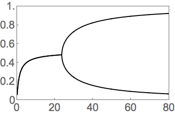
Figure 2: Sigmoidal activation. Learning curves for $K=2$ (a,b) and $K=5$ (c,d). (a,c): order parameters $R$ and $S$ as functions of $\alpha=\beta P/(KN)$. (b,d): the corresponding generalization error $\epsilon_{g}(\alpha).$ Vertical lines indicate the critical values $\alpha_{s}(5)\approx 44.3$ (dotted) and $\alpha_{c}(5)\approx 46.6$ (dashed), while $\alpha_{d}(5)\approx 62.8$ is marked by the short vertical line in (d).

3 Results and Discussion

In the following, we present and discuss our findings for the considered student teacher scenarios and activation functions.

In order to obtain the equilibrium states of the model for given values of $\alpha$ and $K,$ we have minimized the scaled free energy (20) with respect to the site-symmetric order parameters. Potential (local) minima satisfy the necessary conditions

$$\left.{\partial(\beta f)}\right/{\partial R}=\left.{\partial(\beta f)}\right/{\partial C}=\left.{\partial(\beta f)}\right/{\partial S}=0.$$ (21)

In addition, the corresponding Hesse matrix ${\cal H}$ of second derivatives w.r.t.  $R,S,$ and $C$ has to be positive definite. This constitutes a sufficient condition for the presence of a local minimum in the site-symmetric order parameter space. Furthermore, we have confirmed the stability of the local minima against potential deviations from site-symmetry by inspecting the full matrix of second derivatives involving the $(K^{2}\!+\!K(K\!-\!1)/2)$ individual quantities $\left\{R_{ij},Q_{ij}=Q_{ji}\right\}.$

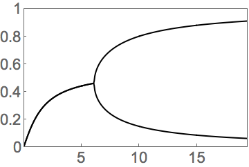
Figure 3: ReLU activation: Learning curves of perfectly matching student teacher scenarios. with $K=2$ (a,b) and $K=10$ (c,d) (a,c): order parameters $R$ and $S$ as a function of $\alpha=\beta P/(KN)$. (b,d): the corresponding generalization error $\epsilon_{g}(\alpha).$ Specialized solutions with $R>S$ are represented by the solid $(R)$ and the dashed line $(S)$ in (c). The dotted line $(S)$ and the chain line $(R)$ represent the local minimum of $\beta f$ with $R<S.$ For $K=2$, the transition occurs at $\alpha_{c}{(2)}\approx 6.1$, (a,b), while $\alpha_{c}(10)\approx 6.2$ (c,d).

3.1 Sigmoidal units re-visited

The investigation of SCM with sigmoidal $g(x)=\mbox{erf}[x/\sqrt{2}]$ with $-1<g(x)<1$ along the lines of the previous section has already been presented in [30]. A similar model with discrete binary weights was studied in [28].

As argued above, for $g(x)=(1+\mbox{erf}[x/\sqrt{2}])$, the mathematical form of the generalization error, Eqs. (11, 26), and the free energy $(\beta f)$ are the same as for the activation $\mbox{erf}[x/\sqrt{2}].$ Hence, the results of [30] carry over without modification. The following summarizes the key findings of the previous study, which we reproduce here for comparison.

For $K\!=\!2$ we observe that $R=S$ in thermal equilibrium for small $\alpha$, see panels (a) and (b) of Fig. 2. Both hidden units perform essentially the same task and acquire equal overlap with both teacher vectors, when trained from relatively small data sets. At a critical value $\alpha_{c}(2)\approx 23.7$, the system undergoes a transition to a specialized state with $R>S$ or $R<S$ in which each hidden unit aligns with one specific teacher unit. Both configurations are fully equivalent due to the invariance of the student output under exchange of the student weights $\mathbf{w}_{1}$ and $\mathbf{w}_{2}$ for $K=2$. The specialization process is continuous with the quantity $|R-S|$ increasing proportional to $(\alpha-\alpha_{c}(K))^{1/2}$ near the transition. This results in a kink in the continuous learning curve $\epsilon_{g}(\alpha)$ at $\alpha_{c}$, as displayed in panel (b) of Figure 2.

Interestingly, a different behavior is found for all $K\geq 3,$ as illustrated for $K=5$ in panels (c) and (d) of Figure 2. The following regimes can be distinguished:

• $0\leq\alpha<\alpha_{s}(K)$:  For small $\alpha,$ the only minimum of $\beta f$ corresponds to unspecialized networks with $R=S$. Within this subspace, a rapid initial decrease of $\epsilon_{g}$ with $\alpha$ is achieved.

• $\alpha_{s}(K)\!\leq\!\alpha\!<\!\alpha_{c}(K)$:  In $\alpha_{s}(K)$, a specialized configuration with $R>S$ appears as a local minimum of the free energy. The $R=S$ configuration corresponds to the global minimum up to $\alpha_{c}(K).$ At this $K$-dependent critical value, the free energies of the competing minima coincide.

• $\alpha\!>\!\alpha_{c}(K)$:  Above $\alpha_{c}$, the configuration with $R>S$ constitutes the global minimum of the free energy and, thus, the thermodynamically stable state of the system. Note that the transition from the unspecialized to the specialized configuration is associated with a discontinuous change of $\epsilon_{g}$, cf. Fig. 2 (d). The $(R>S)$ specialized state facilitates perfect generalization in the limit $\alpha\to\infty.$

• $\alpha\!\geq\!\alpha_{d}(K)$: In addition, at another characteristic value $\alpha_{d},$ the $(R\!=\!S)$ local minimum disappears and is replaced by a negatively specialized state with $R<S$. Note that the existence of this local minimum of the free energy was not reported in [30]. The observed specialization $(S\!-\!R)$ increases linearly with $(\alpha-\alpha_{d})$ for $\alpha\approx\alpha_{d}$. This smooth transition does not yield a kink in $\epsilon_{g}(\alpha).$ A careful analysis of the associated Hesse matrix shows that the $R<S$ state of poor generalization persists for all $\alpha>\alpha_{d}$, indeed.

The limit $K\to\infty$ with $K\ll N$ has also been considered in [30]: The discontinuous transition is found to occur at $\alpha_{s}(K\to\infty)\approx 60.99$ and $\alpha_{c}(K\to\infty)\approx 69.09.$ Interestingly, the characteristic value $\alpha_{d}$ diverges as $\alpha_{d}(K)=4\pi K$ for large $K$ [30]. Hence, the additional transition from $R\!=\!S$ to $R\!<\!S$ cannot be observed for data sets of size $P\propto KN$. On this scale, the unspecialized configuration persists for $\alpha\to\infty.$ It displays site-symmetric order parameters $R=S={\cal O}(1/K)$ with $R,S>0$ and $C={\cal O}(1/K^{2}),$ see [30] for details. Asymptotically, for $\alpha\to\infty,$ they approach the values $R=S=1/K$ and $C=0$ which yields the non-zero generalization error $\epsilon_{g}(\alpha\to\infty)=1/3-1/\pi\approx 0.0150.$ On the contrary, the $R>S$ specialized configuration achieves $\epsilon_{g}\to 0,$ i.e. perfect generalization, asymptotically.

The presence of a discontinuous specialization process for sigmoidal activations with $K\geq 3$ suggests that – in practical training situations – the network will very likely be trapped in an unfavorable configuration unless prior knowledge about the target is available. The escape from the poorly generalizing metastable state with $R=S$ or $R<S$ requires considerable effort in high-dimensional weight space. Therefore, the success of training will be delayed significantly.

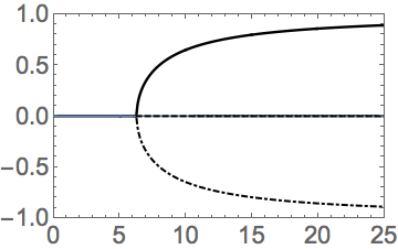
Figure 4: ReLU activation. Learning curves of the perfectly matching student teacher scenario for $K\to\infty$. In this limit, the continuous transition occurs at $\alpha_{c}=2\pi.$ In panel (a), the solid line represents the specialized solution with $R(\alpha)>0$, while the chain line marks the solution with $R(\alpha)<0$. In the former, $S\to 0$ for large $\alpha$, while in the latter, $S$ remains positive with $S={\cal O}(1/K)$ for large $K$. The learning curves $\epsilon_{g}(\alpha)$ for the competing minima of $\beta f$ coincide for $K\to\infty$ as displayed in (b).

3.2 Rectified linear units

In comparison with the previously studied case of sigmoidal activations, we find a surprisingly different behavior in ReLU networks with $K\geq 3.$

For $K\!=\!2$, our findings parallel the results for networks with sigmoidal units: The network configuration is characterized by $R\!=\!S$ for $\alpha<\alpha_{c}(K)$ and specialization increases like

$$|R-S|\propto(\alpha-\alpha_{c}(K))^{1/2}$$ (22)

near the transition. This results in a kink in the learning curve $\epsilon_{g}(\alpha)$ at $\alpha=\alpha_{c}(K)$ as displayed in Fig. 3 (a,b) for $K=2$ with $\alpha_{c}(2)\approx 6.1.$

However, in ReLU networks, the transition is also continuous for $K\!\geq\!3$. Panels (c,d) of Fig. 3 display the example case $K=10$ with $\alpha_{c}({10})\approx 6.2$.

The student output is invariant under exchange of the hidden unit weight vectors, consistent with an unspecialized state for small $\alpha.$ At a critical value $\alpha_{c}(K)$ the unspecialized $(R=S)$ configuration is replaced by two minima of $\beta f$: in the global minimum we have $R>S$, while the competing local minimum corresponds to configurations with $R<S.$ Only the former facilitates perfect generalization with $R\to 1,S\to 0$ in the limit $\alpha\to\infty.$ In both competing minima the emerging specialization follows Eq. (22) with critical exponent $1/2.$

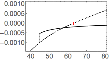
Figure 5: Student cross overlap $C$. (a) Sigmoidal activations, here $K=5$. The values $\alpha_{s},\alpha_{c},\alpha_{d}$ are marked as in Fig. 2 (c). For better visibility of the behavior near $\alpha_{c}$, only a small range of $\alpha$ is shown. (b) ReLU system with $K=10$ as an example.

In contrast to the case of sigmoidal activation, both competing configurations of the ReLU system display very similar generalization behavior. While, in general, only states with $R>0$ can perfectly reproduce the teacher output, the student configurations with $S>0$ and $R<0$ also achieve relatively low generalization error for large $\alpha$, see Fig. 3 (c,d) for an example.

The limiting case of large networks with $K\!\to\!\infty$ can be considered explicitly. We find for large ReLU networks that the continuous specialization transition occurs at

$$\alpha_{c}(K\!\to\!\infty)=2\pi\approx 6.28.$$

The generalization error decreases very rapidly (instantaneously on $\alpha$-scale) from the initial value of $\epsilon_{g}(0)\approx 0.341$ with $R\!=\!S\!=\!C\!=\!0$ to a plateau with

$$\epsilon_{g}(\alpha)\!=\!\textstyle\frac{1}{4}\!-\!\frac{1}{2\pi}\approx 0.091\mbox{~{}for~{}}0<\alpha<2\pi$$

where $R\!=\!S\!=\!1/K\mbox{~{}~{}and~{}~{}}C\!=\!{\cal{O}}(1/K^{2}).$ For $\alpha>\alpha_{c}$, the order parameter $R$ either increases or decreases with $\alpha$, approaching the values $R\to\!\pm 1$ asymptotically, while $S(\alpha)=0$ in both branches for $K\to\infty.$

Surprisingly, both solutions display the exact same generalization error, see Fig. 4 (b). Consequently, the free energies $\beta f$ of the competing minima also coincide in the limit $K\to\infty$ since the entropy (17) satisfies $S(-R,0,0)=S(R,0,0).$

In the configuration with $R<0$ the order parameters display the scaling

$$S={\cal O}\left(1/{K}\right)\mbox{~{}~{}and~{}~{}}C={\cal O}\left(1/{K^{2}}\right)$$ (23)

for large $K.$ In A.4 we show how a single teacher ReLU with activation $\max(0,x^{*})$ can be approximated by $(K-1)$ weakly aligned units in combination with one anti-correlated student node. While the former effectively approximates a linear response of the form $const.\ +x^{*}$, the unit with $R=-1$ implements $\max(0,-x^{*})$. Since $\max(0,x^{*})=\max(0,-x^{*})+x^{*}$ the student can approximate the teacher output very well, see also the appendix for details. In the limit $K\to\infty$, the correspondence becomes exact and facilitates perfect generalization for $\alpha\to\infty.$

Note that a similar argument does not hold for student teacher scenarios with sigmoidal activation functions, as they not display the partial linearity of the ReLU.

3.3 Student-student overlaps

It is also instructive to inspect the behavior of the order parameter $C$ which quantifies the mutual overlap of student weight vectors. In the ReLU system with large finite $K$, we observe $C(\alpha)={\cal O}(1/K^{2})>0$ before the transition. It reaches a maximum value at the phase transition and decreases with increasing $\alpha>\alpha_{c}$. In the positively specialized configuration it approaches the limiting value $C(\alpha\to\infty)=0$ from above, while it assumes negative values on the order ${\cal O}(1/K^{2})$ in the configuration with $R<S.$

This is in contrast to networks of sigmoidal units, where $C<0$ before the discontinuous transition and in the specialized $(R>S)$ state, see [30, 31] for details. Interestingly, the characteristic value $\alpha_{d}$ coincides with the point where $C$ becomes positive in the suboptimal local minimum of $\beta f.$

Figure 5 displays $C(\alpha)$ for sigmoidal (panel a) and ReLU activation (b) for $K=5$ as an example. Apparently the ReLU system tends to favor correlated hidden units in most of the training process.

3.4 Monte Carlo simulations

In order to demonstrate that our theoretical results also apply qualitatively in finite systems and beyond the high-temperature limit, we performed Monte Carlo simulations of the training processes.

We have implemented the student teacher scenarios in relatively small systems with $N=50$ and $K=4$ hidden units. The systems were trained according to a Metropolis-like scheme with continuous changes of the student weights. In an individual Monte Carlo step (MCS), all adaptive weights in the student network were subject to independent, zero mean additive Gaussian noise with subsequent normalization to maintain $\mathbf{w}_{j}^{2}=N$ for all $j.$ The associated change $\Delta E$ of the training energy $E$, Eq. (7), was computed and the randomized modification was accepted with probability $\min\{1,e^{-\beta\Delta E}\}.$ A constant variance of the Gaussian noise was selected as to maintain acceptance rates in the vicinity of $0.5$ in each setting.

All simulations were performed with $\beta=1,$ which corresponds to a relatively low training temperature, and with training set sizes $P=\widetilde{\alpha}KN$ that could be handled with moderate computational effort.

In principle, all stable and metastable states, i.e. local and global minima of the associated free energy, would eventually be visited starting from arbitrary initializations by the finite system. However, this requires very large equilibration and observation times. Therefore we followed an alternative strategy by preparing initial states which slightly favored one of the competing configurations and observed the quasi-stationary behavior of the system at intermediate training times. In all training processes, quasistationary states could be observed after ${\cal O}(10^{4})$ elementary MCS. Below the specialization transition, the systems approach unspecialized states independent of the initialization. Averages and standard deviations were determined over the last $1000$ MCS in 20 independent runs for each considered setting.

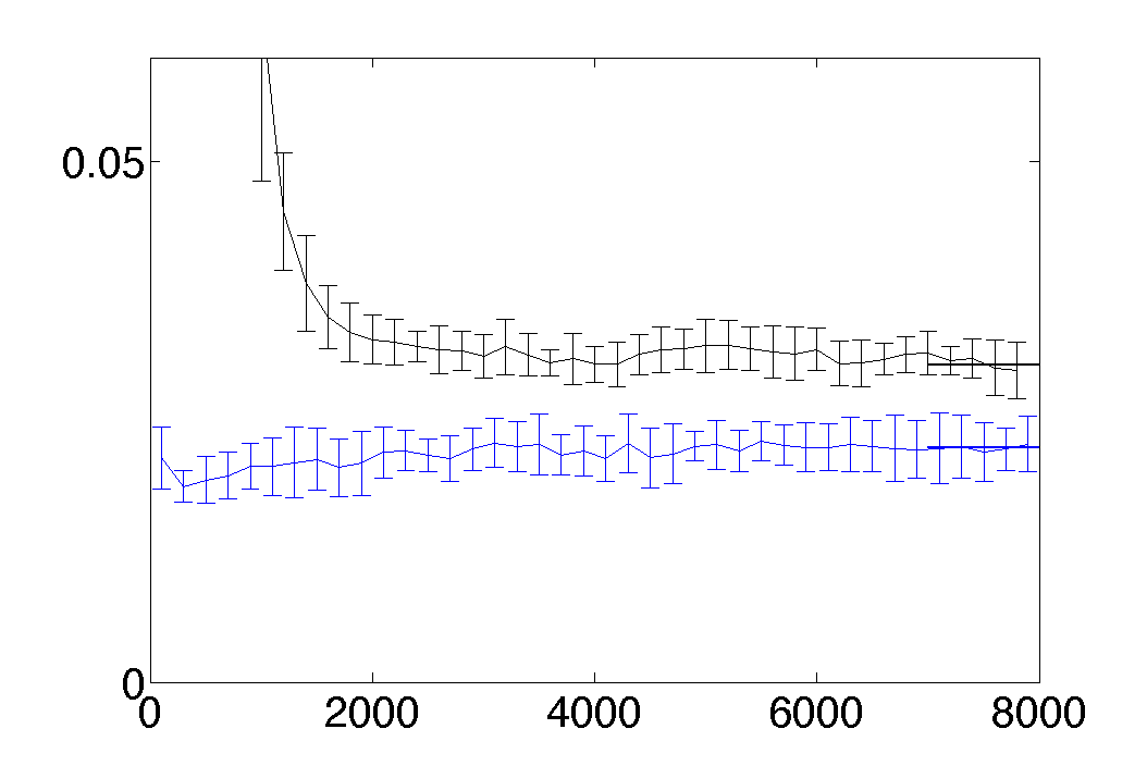
Figure 6: Monte Carlo simulations of the ReLU system. (a) the generalization error as observed with $N=50,\beta=1,K=4$ for $\widetilde{\alpha}=24$ on average over 20 independent runs, error bars represent the standard deviations. (b,c) histograms of the relative frequency of values $R_{im}$ observed over the last 1000 elementary Monte Carlo steps as marked by the bold solid lines in (a). The upper curve in (a) and histogram (b) correspond to initializations of the systems in slighlty anti-specialized states. For the lower curve and histogram (c) the systems were initialized with a weak positive specialization, see Sec. 3.4.

Fig. 6 shows example learning curves in the ReLU system with $K=4$ and training set size $\widetilde{\alpha}=24,$ which is sufficient for hidden unit specialization. The last 1000 MCS are marked by bold solid lines in panel (a). The simulations confirm the existence of two competing quasistationary states. Histograms of the observed order parameters $R_{im}$ show that they correspond to a specialized state with few, large positive student teacher overlaps, see Fig. 6 (c). The anti-specialized state is characterized by a considerable fraction of values $R_{im}<0$, see panel (b). We also obtained results for the system with sigmoidal activation, which are not displayed here, confirming the competition of a specialized state with unspecialized configurations. Similar findings, including histograms of the observed $R_{im},$ have been published in [30] for sigmoidal units only. There, the authors also present simulation results for $K=2.$

We determined the average generalization error from the order parameter values as observed in the competing quasistationary states of training in the last 1000 MCS. Figure 7 displays the corresponding generalization error as a function of $\widetilde{\alpha}$ for sigmoidal activation in panel (a) and for a ReLU hidden layer in (b). The observed behavior is consistent with the predicted discontinuous and continuous phase transition, respectively. In particular we note that the competing configurations in the ReLU system (panel b) display very similar generalization errors. In contrast, the difference between specialized and unspecialized sigmoidal networks is much more pronounced, see panel (a) of Fig. 7.

While the simulations were performed in fairly small systems and with $\beta=1$, the results are in very good qualitative agreement with the theoretical predictions obtained in the limits $N\to\infty$ and $\beta\to 0.$ Note that at low temperature, training and generalization error are not identical. As expected $E/P$ is found to be systematically lower than $\epsilon_{g}$. However, we observed that generalization and training error evolve in parallel with the training time (MCS) and display analogous dependencies on the training set size $\widetilde{\alpha}$. Details will be presented elsewhere.

3.5 Practical relevance

It is important to realize that a quantitative comparison of the two scenarios, for instance w.r.t. the critical values $\alpha_{c}$, is not sensible. The complexities of sigmoidal and ReLU networks with $K$ units do not necessarily correspond to each other. Moreover, the actual $\alpha$-scale is trivially related to a potential scaling of the activation functions.

However, our results provide valuable qualitative insight: The continuous nature of the transition suggests that ReLU systems should display favorable training behavior in comparison to systems of sigmoidal units. In particular, the suboptimal competing state displays very good performance, comparable to that of the properly specialized configuration. Their generalization abilities even coincide in large networks of many hidden units.

On the contrary, the achievement of good generalization in networks of sigmoidal units will be delayed significantly due to the discontinuous specialization transition which involves a poorly generalizing metastable state.

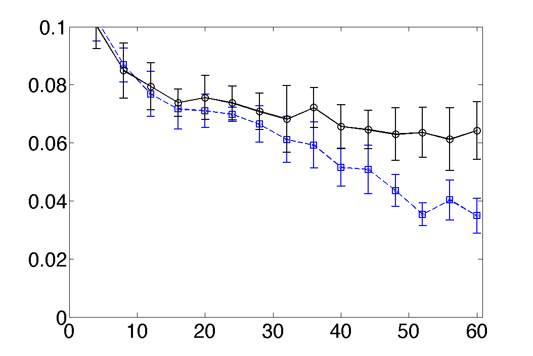
Figure 7: Monte Carlo simulations of the student teacher scenarios. The generalization error as observed for systems with $N=50,\beta=1,K=4$ as a function of $\widetilde{\alpha}.$ Averages and standard deviations (20 independent simulation runs) of $\epsilon_{g}$ were determined over the last 1000 Monte Carlo steps. (a) networks with sigmoidal activation in unspecialized (upper) and specialized configurations (lower curve). (b) systems with ReLU hidden layer in anti-specialized (upper) or specialized (lower) quasistationary states.

4 Conclusion and Outlook

We have investigated the training of shallow, layered neural networks in student teacher scenarios of matching complexity. Large, adaptive networks have been studied by employing modelling concepts and analytical tools borrowed from the statistical physics of learning. Specifically, stochastic training processes at high formal temperature were studied and learning curves were obtained for two popular types of hidden unit activation. Monte Carlo simulations confirm our findings qualitatively. To the best of our knowledge, this work constitutes the first theoretical, model-based comparison of sigmoidal activations and rectified linear units in feed-forward neural networks.

Our results confirm that networks with $K\geq 3$ sigmoidal hidden units undergo a discontinuous transition: A critical training set size is required to facilitate the differentiation, i.e. specialization of hidden units. However, a poorly performing state of the network persists as a locally stable configuration for all sizes of the training set. The presence of such an unfavorable local minimum will delay successful learning in practice, unless prior knowledge of the target rule allows for non-zero initial specialization.

On the contrary, the specialization transition is always continuous in ReLU networks. We show that above a weakly $K$-dependent critical value of the re-scaled training set size $\alpha$, two competing specialized configurations can be assumed. Only one of them displays positive specialization $R>S$ and facilitates perfect generalization from large training sets for finite $K$. However, the competing configuration with negative specialization $R<0,S>0$ realizes similar performance which is nearly identical for networks with many hidden units and coincides exactly in the limit $K\to\infty.$

As a consequence, the problem of retarded learning [27] associated with the existence of metastable configurations is expected to be less pronounced in ReLU networks than in their counterparts with sigmoidal activation.

Clearly, our approach is subject to several limitations which will be addressed in future studies. Probably the most straightforward, relevant extension of our work would be the consideration of further activation functions, for instance modifications of the ReLU such as the leaky or noisy ReLU or alternatives like swish and max-out [10, 9].

Within the site-symmetric space of configurations, cf. Eq. (10), only the specialization of single units with respect to one of the teacher units can be considered. In large networks, one would expect partially specialized states, where subsets of hidden units achieve different alignment with specific teacher units. Their study requires the extension of the analysis beyond the assumption of site-symmetry.

Training at low formal temperatures can be studied along the lines of [31] where the replica formalism was already applied to networks with sigmoidal activation. Alternatively, the simpler annealed approximation could be used [3, 17, 18]. Both approaches allow to vary the control parameter $\beta$ of the training process and the scaled example set size $\widetilde{\alpha}=P/(KN)$ independently, as it is the case in more realistic settings. Note that the findings reported in [31] for sigmoidal activation displayed excellent qualitative agreement with the results of the much simpler high-temperature analysis in [30].

The dynamics of non-equilibrium on-line training by gradient descent has been studied extensively for soft-committee-machines with sigmoidal activation, e.g. [23, 24, 25, 26]. There, quasi-stationary plateau states in the learning dynamics are the counterparts of the phase transitions observed in thermal equilibrium situations. First results for ReLU networks have been obtained recently [45]. These studies should be extended in order to identify and understand the influence of the activation function on the training dynamics in greater detail.

Model scenarios with mismatched student and teacher complexity will provide further insight into the role of the activation function for the learnability of a given task. It should be interesting to investigate specialization transitions in practically relevant settings in which either the task is unlearnable $(K<M)$ or the student architecture is over-sophisticated for the problem at hand ($K>M$). In addition, student and teacher systems with mismatched activation functions should constitute interesting model systems.

The complexity of the considered networks can be increased in various directions. If the simple shallow architecture of Eq. (1) is extended by local thresholds and hidden to output weights that are both adaptive, it parameterizes a universal approximator, see e.g. [46, 47, 48]. Decoupling the selection of these few additional parameters from the training of the input to hidden weights should be possible following the ideas presented in [49].

Ultimately, deep layered architectures should be investigated along the same lines. As a starting point, simplifying tree-like architectures could be considered as in e.g. [27, 39].

Our modelling approach and theoretical analysis goes beyond the empirical investigation of data set specific performance. The suggested extensions bear the promise to contribute to a better, fundamental understanding of layered neural networks and their training behavior.

Appendix A Mathematical Details

A.1 Co-variance matrix and order parameters

The $(K\!+\!M)\!\times\!(K\!+\!M)$-dim. matrix of order parameters reads

$${\cal C}=\left[\begin{array}[]{cc}{T}&{R}\\ R^{\top}&Q\end{array}\right]\mbox{~{}with submatrices~{}}T\!\in\!\mathbb{R}^{M\times M},R\!\in\!\mathbb{R}^{K\times M},Q\!\in\!\mathbb{R}^{K\times K}$$ (24)

of elements $T_{ij}\!=\!\left\langle x^{*}_{i}x^{*}_{j}\right\rangle\!=\!\frac{\mathbf{w}_{i}^{*}\cdot\mathbf{w}_{j}^{*}}{N}$, $R_{ij}\!\!=\!\left\langle x_{i}x^{*}_{j}\right\rangle\!=\!\frac{\mathbf{w}_{i}\cdot\mathbf{w}_{j}^{*}}{N},$ and $Q_{ij}=\!\left\langle x_{i}x_{j}\right\rangle\!=\!\frac{\mathbf{w}_{i}\cdot\mathbf{w}_{j}}{N}.$ Note that Eqs. (18) and (19) correspond to the special case of $K=M$ and exploit site-symmetry (10) and normalization (6).

A.2 Derivation of the generalization error

Here we give a derivation of the generalization error in terms of the order parameters for sigmoidal and ReLU student and teacher. For general $K$ and $M$ it reads

$$\epsilon_{g}=\frac{1}{2K}\Bigg{(}\sum_{i,j=1}^{K}\langle g(x_{i})g(x_{j})\rangle-2\sum_{i=1}^{K}\sum_{j=1}^{M}\langle g(x_{i})g(x_{j}^{*})\rangle\,\,+\sum_{i,j=1}^{M}\langle g(x_{i}^{*})g(x_{j}^{*})\rangle\Bigg{)},$$ (25)

which reduces to Eq. (9) for $K=M.$ To obtain $\epsilon_{g}$ for a particular choice of activation function $g$, expectation values of the form $\left\langle g(x)g(y)\right\rangle$ have to be evaluated over the joint normal density of the hidden unit local potentials $x$ and $y$, i.e.  $P(x,y)=\mathcal{N}(\mathbf{0},\widehat{\mathcal{C}})$ with the appropriate submatrix $\widehat{\mathcal{C}}$ of ${\cal C}$, cf. Eq. (24):

$$\widehat{\mathcal{C}}=\left[\begin{array}[]{cc}\left\langle y^{2}\right\rangle&\left\langle xy\right\rangle\\ \left\langle xy\right\rangle&\left\langle x^{2}\right\rangle\end{array}\right].$$

A.2.1 Sigmoidal

For student and teacher with sigmoidal activation functions $g(x)=\mbox{erf}\big{[}\frac{x}{\sqrt{2}}\big{]}$ or $g(x)=\left(1+\mbox{erf}\big{[}\frac{x}{\sqrt{2}}\big{]}\right)$, the generalization error has been derived in [24]:

$$\epsilon_{g} = \frac{1}{\pi}\left\{\sum_{i,j=1}^{K}\sin^{-1}\frac{Q_{ij}}{\sqrt{1+Q_{ii}}\sqrt{1+Q_{jj}}}\right.+\sum_{n,m=1}^{M}\sin^{-1}\frac{T_{nm}}{\sqrt{1+T_{nn}}\sqrt{1+T_{mm}}}$$ (26)

$$-\textstyle\left.2\sum_{i=1}^{K}\sum_{j=1}^{M}\sin^{-1}\frac{R_{ij}}{\sqrt{1+Q_{ii}}\sqrt{1+T_{jj}}}\right\}.$$

A.2.2 ReLU

For student and teacher with ReLU activations $g(x)=\mbox{max}\{0,x\}$, applying the elegant formulation used in [50] gives an analytic expression for the two-dimensional integrals: $\langle g(x)g(y)\rangle=\left\langle\mbox{max}\{0,x\}\mbox{max}\{0,y\}\right\rangle$

$$\textstyle=\int\limits_{0}^{\infty}\int\limits_{0}^{\infty}xy\mathcal{N}(\mathbf{0},\widehat{\mathcal{C}})dxdy=\frac{\widehat{\mathcal{C}}_{12}}{4}+\left.{\sqrt{\widehat{\mathcal{C}}_{11}\widehat{\mathcal{C}}_{22}-\widehat{\mathcal{C}}_{12}^{2}}+\widehat{\mathcal{C}}_{12}\sin^{-1}\left[\frac{\widehat{\mathcal{C}}_{12}}{\sqrt{\widehat{\mathcal{C}}_{11}\widehat{\mathcal{C}}_{22}}}\right]}\right/{2\pi}.$$ (27)

Substituting the result from Eq. (27) in Eq. (25) for the corresponding covariance matrices gives the analytic expression for the generalization error in terms of the order parameters:

$$\epsilon_{g} = \frac{1}{2K}\sum_{i,j=1}^{K}\left(\frac{Q_{ij}}{4}\!+\!\frac{\sqrt{Q_{ii}Q_{jj}\!-\!Q_{ij}^{2}}\!+\!Q_{ij}\sin^{-1}\left[\frac{Q_{ij}}{\sqrt{Q_{ii}{Q_{jj}}}}\right]}{2\pi}\right)$$ (29)

$$-\frac{1}{K}\sum_{i=1}^{K}\sum_{j=1}^{M}\textstyle\left(\frac{R_{ij}}{4}\!+\!\frac{\sqrt{Q_{ii}T_{jj}\!-\!R_{ij}^{2}}\!+\!R_{ij}\sin^{-1}\left[\frac{R_{ij}}{\sqrt{Q_{ii}T_{mm}}}\right]}{2\pi}\right)$$

$$+\frac{1}{2K}\sum_{i,j=1}^{M}\textstyle\left(\frac{T_{ij}}{4}\!+\!\frac{\sqrt{T_{ii}T_{jj}\!-\!T_{ij}^{2}}\!+\!T_{ij}\sin^{-1}\left[\frac{T_{ij}}{\sqrt{T_{ii}T_{jj}}}\right]}{2\pi}\right).$$

For $K=M$, orthonormal teacher vectors with $T_{ij}=\delta_{ij}$, fixed student norms $Q_{ii}=1$, and assuming site symmetry, Eq. (10), we obtain Eqs. (11) and (2.3), respectively.

A.3 Single unit student and teacher

In the simple case $K=1$ with a single unit as student and teacher network, we have to consider only one order parameter $R=\mathbf{w}\cdot\mathbf{w}^{*}/N.$ Assuming $\mathbf{w}\cdot\mathbf{w}=\mathbf{w}^{*}\cdot\mathbf{w}^{*}=N,$ we obtain the free energy $\beta f=\alpha\,\epsilon_{g}-s$ with

$$s = \frac{1}{2}\ln[1-R^{2}]\,+\,const.\ \hfill\$$ (30)

$$\epsilon_{g} = \frac{1}{3}-\frac{2}{\pi}\sin^{-1}\left[{R}\big{/}{2}\right]\mbox{~{}~{}~{}~{}~{}~{}~{}~{}~{}~{}~{}~{}~{}(sigmoidal)~{}~{}~{}}$$ (31)

$$\epsilon_{g} = \frac{2\!-\!R}{4}\!-\!\frac{\sqrt{1\!-\!R^{2}}\!+\!R\sin^{-1}[R]}{2\pi}\hfill\mbox{~{}~{}~{}~{}~{}(ReLU).~{}~{}}$$ (32)

The necessary condition $\partial{(\beta f)}/{\partial R}{=}0$ becomes

$$\alpha = \frac{\pi R\sqrt{4-R^{2}}}{2(1-R^{2})}\hfill\mbox{~{}~{}~{}~{}~{}~{}~{}~{}~{}~{}~{}~{}~{}~{}~{}~{}~{}~{}(sigmoidal)~{}}$$ (33)

$$\alpha = \frac{4\pi R}{(1-R^{2})(\pi+2\sin^{-1}[R])}\hfill\mbox{~{}~{}~{}~{}~{}~{}~{}(ReLU).}$$ (34)

In both cases, the student teacher overlap increases smoothly from zero to $R=1.$ A Taylor expansion of $1/\alpha$ for $R\approx 1$ yields the asymptotic behavior

$$R(\alpha)=1-\frac{const.}{\alpha}\mbox{~{}~{}and~{}~{}}\epsilon_{g}(\alpha)=\frac{1}{2\alpha}\mbox{~{}~{}for ~{}}\alpha\to\infty$$

for both types of activation. This basic large-$\alpha$ behavior with $\epsilon_{g}\propto\alpha^{-1}$ carries over to the specialized solutions for settings with $K\!=\!M.$

A.4 Weak and negative alignment

Here we consider a particular teacher unit which realizes a ReLU response $\max(0,x^{*})\mbox{~{}with~{}}x^{*}=\mathbf{w}^{*}\cdot\boldsymbol{\xi}/\sqrt{N}.$ A set of $K$ hidden units in the student network can obviously reproduce the response by aligning one of the units perfectly with, e.g., $R\!=\!\mathbf{w}_{1}\cdot\mathbf{w}^{*}/N\!=\!1$ and $S\!=\!\mathbf{w}_{j}\cdot\mathbf{w}^{*}/N\!=\!0$ for $j>1$. Similarly, we obtain for $R=-1$ that $x_{1}=-\mathbf{w}^{*}\cdot\boldsymbol{\xi}\mbox{~{}~{}and~{}}\max(0,x_{1})=\max(0,-x^{*}).$

Now consider the mean response of a student unit with small positive overlap $S=\mathbf{w}_{j}\cdot\mathbf{w}^{*}/N$, given the teacher unit response $x^{*}$. It corresponds to the average $\left\langle g(x_{j})\right\rangle_{x^{*}}$ over the conditional density $P(x_{j}|x^{*})=P(x_{j},x^{*})/P(x^{*})$. One obtains

$$\left\langle g(x_{j})\right\rangle_{x^{*}}=\,{1}/{\sqrt{2\pi}}+{S}\,x^{*}/2+{\cal O}(S^{2})$$

by means of a Taylor expansion for $S\approx 0$. As a special case, the mean response of an orthogonal unit with $S=0$ is $1/\sqrt{2\pi},$ independent of $x^{*}.$

It is straightforward to work out the conditional average of the total student response for a particular order parameter configuration with $R=-1$ and $S={2}/{(K-1)}.$ Apart from the prefactor $1/\sqrt{K}$ it is given by

$$\max(-x^{*},0)+x^{*}+\textstyle\frac{K-1}{\sqrt{2\pi}}=\max(0,x^{*})+\frac{K-1}{\sqrt{2\pi}},$$

where the right hand side coincides with the expected output for $R=1$ and $S=0.$ Hence, the average response agrees with the teacher output for large $K$. Moreover, the correspondence becomes exact in the limit $K\to\infty,$ which facilitates perfect generalization in the negatively specialized state with $S>0,R<0$ discussed in Section 3.

References

References

- [1] J. Hertz, A. Krogh, R. Palmer, Introduction To The Theory Of Neural Computation, Addison-Wesley, Reading, MA, USA, 1991.
- [2] C. Bishop, Neural Networks for Pattern Recognition, Oxford University Press, Inc., New York, NY, USA, 1995.
- [3] A. Engel, C. van den Broeck, The Statistical Mechanics of Learning, Cambridge University Press, Cambridge, UK, 2001.
- [4] T. Hastie, R. Tibshirani, J. Friedman, The Elements of Statistical Learning, Springer Series in Statistics, Springer, New York, NY, USA, 2001.
- [5] C. Bishop, Pattern Recognition and Machine Learning (Information Science and Statistics), Springer, Heidelberg, Germany, 2006.
- [6] I. Goodfellow, Y. Bengio, A. Courville, Deep Learning, MIT Press, Cambridge, MA, USA, 2016.
- [7] Y. LeCun, Y. Bengio, G. Hinton, Deep learning, Nature 521 (2015) 436–444.
- [8] P. Angelov, A. Sperduti, Challenges in Deep Learning, in: M. Verleysen (Ed.), Proc. of the European Symposium on Artificial Neural Networks (ESANN), i6doc.com, 2016, pp. 489–495.
- [9] P. Ramachandran, B. Zoph, Q. V. Le, Searching for activation functions, ArXiv abs/1710.05941, Presented at: Sixth Intl. Conf. on Learning Representations, ICLR 2018 (2017).
- [10] S. Eger, P. Youssef, I. Gurevych, Is it Time to Swish? Comparing Deep Learning Activation Functions Across NLP tasks, in: Proceedings of the 2018 Conference on Empirical Methods in Natural Language Processing, Association for Computational Linguistics, Brussels, Belgium, 2018, pp. 4415–4424.
- [11] A. L. Maas, A. Y. Hannun, A. Y. Ng, Rectifier nonlinearities improve neural network acoustic models, in: Proc. 30th ICML Workshop on Deep Learning for Audio, Speech and Language Processing, 2013.
- [12] R. Hahnloser, R. Sarpeshkar, M. Mahowald, R. Douglas, S. Seung, Digital selection and analogue amplification coexist in a cortex-inspired silicon circuit, Nature 405 (2000) 947–951.
- [13] A. Krizhevsky, I. Sutskever, G. E. Hinton, Imagenet classification with deep convolutional neural networks, in: Proceedings of the 25th International Conference on Neural Information Processing Systems (NIPS) - Volume 1, Curran Assoc. Inc., USA, 2012, pp. 1097–1105.
- [14] V. Nair, G. Hinton, Rectified linear units improve restricted Boltzmann machines, in: Proc. 27th International Conference on Machine Learning (ICML), Omnipress, USA, 2010, pp. 807–814.
- [15] T. Villmann, J. Ravichandran, A. Villmann, D. Nebel, M. Kaden, Investigation of Activation Functions for Generalized Learning Vector Quantization, in: A. Vellido, K. Gibert, C. Angulo, J. Martín Guerrero (Eds.), Advances in Self-Organizing Maps, Learning Vector Quantization, Clustering and Data Visualization, WSOM 2019, Vol. 976 of Advances in Intelligent Systems and Computing, Springer, Cham, 2019, pp. 179–188.
- [16] X. Glorot, A. Bordes, Y. Bengio, Deep Sparse Rectifier Neural Networks, in: G. Gordon, D. Dunson, M. Dudík (Eds.), Proceedings of the Fourteenth International Conference on Artificial Intelligence and Statistics, Vol. 15 of Proceedings of Machine Learning Research, PMLR, Fort Lauderdale, FL, USA, 2011, pp. 315–323.
- [17] H. S. Seung, H. Sompolinsky, N. Tishby, Statistical mechanics of learning from examples, Phys. Rev. A 45 (1992) 6056–6091.
- [18] T. L. H. Watkin, A. Rau, M. Biehl, The statistical mechanics of learning a rule, Rev. Mod. Phys. 65 (2) (1993) 499–556.
- [19] W. Kinzel, Phase transitions of neural networks, Philosophical Magazine B 77 (5) (1998) 1455–1477.
- [20] M. Opper, Learning and generalization in a two-layer neural network: The role of the Vapnik-Chervonenkis dimension, Phys. Rev. Lett. 72 (1994) 2113–2116.
- [21] M. Biehl, N. Caticha, The statistical mechanics of on-line learning and generalization, in: M. Arbib (Ed.), The Handbook of Brain Theory and Neural Networks, MIT Press, Cambridge, MA, 2003, pp. 1095–1098.
- [22] M. Biehl, H. Schwarze, Learning by on-line gradient descent, J. Phys. A: Mathematical and General 28 (1995) 643–656.
- [23] D. Saad, S. A. Solla, Exact solution for on-line learning in multilayer neural networks, Phys. Rev. Lett. 74 (1995) 4337–4340.
- [24] D. Saad, S. Solla, On-line learning in soft committee machines, Phys. Rev. E 52 (4) (1995) 4225–4242.
- [25] M. Biehl, P. Riegler, C. Wöhler, Transient dynamics of on-line learning in two-layered neural networks, J. Phys. A: Mathematical and General 29 (1996) 4769–4780.
- [26] R. Vicente, N. Caticha, Functional optimization of online algorithms in multilayer neural networks, J. Phys. A: Math. and Gen. 30 (17) (1997) L599–L605.
- [27] D. Herschkowitz, M. Opper, Retarded Learning: Rigorous Results from Statistical Mechanics, Phys. Rev. Lett. 86 (2001) 2174–2177.
- [28] K. Kang, J.-H. Oh, C. Kwon, Y. Park, Generalization in a two-layer neural network, Phys. Rev. E 48 (1993) 4805–4809.
- [29] M. Biehl, M. Ahr, E. Schlösser, Statistical physics of learning: phase transitions in multilayered neural networks, in: B. Kramer (Ed.), Advances in Solid State Physics, Vol. 40, Vieweg, 2000, pp. 819–826.
- [30] M. Biehl, E. Schlösser, M. Ahr, Phase transitions in soft-committee machines, Europhysics Letters 44 (1998) 261–267.
- [31] M. Ahr, M. Biehl, R. Urbanczik, Statistical physics and practical training of soft-committee machines, The European Physical Journal B-Condensed Matter and Complex Systems 10 (3) (1999) 583–588.
- [32] L. Saitta, A. Giordana, A. Cornuéjols, Phase Transitions in Machine Learning, Cambridge University Press, Cambridge, UK, 2011.
- [33] S. Cocco, R. Monasson, L. Posani, S. Rosay, J. Tubiana, Statistical physics and representations in real and artificial neural networks, Physica A: Stat. Mech. and its Applications 504 (2018) 45–76.
- [34] J. Kadmon, H. Sompolinsky, Optimal Architectures in a Solvable Model of Deep Networks, in: Advances in Neural Information Processing Systems (NIPS 29), Curran Assoc. Inc., 2016, pp. 4781–4789.
- [35] M. Pankaj, A. Lang, D. Schwab, An exact mapping from the Variational Renormalization Group to Deep Learning, arXiv repository [stat.ML] (1410.3831v1) (2014).
- [36] J. Sohl-Dickstein, E. Weiss, N. Maheswaranathan, S. Ganguli, Deep unsupervised learning using non-equilibrium thermodynamics, Proc. of Machine Learning Research 37 (2016) 2256–2265.
- [37] N. Caticha, R. Calsaverini, R. Vicente, Phase transition from egalitarian to hierarchical societies driven between cognitive and social constraints, arXiv repository (1608.03637) (2016).
- [38] M. Biehl, N. Caticha, M. Opper, T. Villmann, Statistical physics of learning and inference, in: M. Verleysen (Ed.), 27th European Symposium on Artificial Neural Networks, Computational Intelligence and Machine Learning (ESANN), i6doc.com, 2019, pp. 501–509.
- [39] C. Baldassi, E. Malatesta, R. Zecchina, On the geometry of solutions and on the capacity of multi-layer neural networks with relu activations, arXiv preprint arXiv:1907.07578 (2019).
- [40] S. Goldt, M. Mézard, F. Krzakala, L. Zdeborová, Modelling the influence of data structure on learning in neural networks, arXiv e-print arXiv:1909.11500 (2019).
- [41] Y. Dauphin, R. Pascanu, C. Gulcehre, K. Cho, S. Ganguli, Y. Bengio, Identifying and attacking the saddle point problem in high-dimensional non-convex optimization, in: Z. Ghahramani, M. Welling, C. Cortes, N. Lawrence, K. Weinberger (Eds.), Advances in Neural Information Processing Systems (NIPS 27), Curran Assoc. Inc., 2014, pp. 2933–2941.
- [42] A. M. Saxe, J. L. McClelland, S. Ganguli, Exact solutions to the nonlinear dynamics of learning in deep linear neural networks, in: Y. Bengio, Y. LeCun (Eds.), 2nd International Conference on Learning Representations (ICLR), Conference Track Proceedings, 2014.
- [43] R. Urbanczik, Storage capacity of the fully-connected committee machine, J. Phys. A: Mathematical and General 30 (11) (1997) L387–L392.
- [44] H. Schwarze, J. Hertz, Generalization in fully connected committee machines, Europhysics Letters 21 (7) (1993) 785–790.
- [45] M. Straat, M. Biehl, On-line learning dynamics of ReLU neural networks using statistical physics techniques, in: M. Verleysen (Ed.), 27th Europ. Symp. on Artificial Neural Networks, Computational Intelligence and Machine Learning (ESANN), i6doc.com, 2019, pp. 517–522.
- [46] G. Cybenko, Approximations by superpositions of sigmoidal functions, Mathematics of Control, Signals, and Systems 2 (4) (1989) 303–314.
- [47] K. Hornik, Approximation Capabilities of Multilayer Feedforward Networks, Neural Networks 4 (2) (1991) 251–257.
- [48] B. Hanin, Universal Function Approximation by Deep Neural Nets with Bounded Width and ReLU Activations, arXiv e-print 1708.02691 (2017).
- [49] D. Endres, P. Riegler, Learning dynamics on different timescales, J. Phys. A: Math. and Gen. 32 (49) (1999) 8655–8663.
- [50] Y. Yoshida, R. Karakida, M. Okada, S. Amari, Statistical Mechanical Analysis of Online Learning with Weight Normalization in Single Layer Perceptron, Journal of the Physical Society of Japan 86 (4) (2017) 044002.