Localization transition in the Discrete Non-Linear Schrödinger Equation:
ensembles inequivalence and negative temperatures.

Abstract

We present a detailed account of a first-order localization transition in the Discrete Nonlinear Schrödinger Equation, where the localized phase is associated to the high energy region in parameter space. We show that, due to ensemble inequivalence, this phase is thermodynamically stable only in the microcanonical ensemble. In particular, we obtain an explicit expression of the microcanonical entropy close to the transition line, located at infinite temperature. This task is accomplished making use of large-deviation techniques, that allow us to compute, in the limit of large system size, also the subleading corrections to the microcanonical entropy. These subleading terms are crucial ingredients to account for the first-order mechanism of the transition, to compute its order parameter and to predict the existence of negative temperatures in the localized phase. All of these features can be viewed as signatures of a thermodynamic phase where the translational symmetry is broken spontaneously due to a condensation mechanism yielding energy fluctuations far away from equipartition: actually they prefer to participate in the formation of nonlinear localized excitations (breathers), typically containing a macroscopic fraction of the total energy.

I Introduction

Beyond its phenomenological interest for many physical applications, such as Bose-Einstein condensates in optical lattices Trombettoni and Smerzi (2001); Franzosi et al. (2011) or light propagating in arrays of optical waveguides Eisenberg et al. (1998), in the last decades the Discrete Nonlinear Schrödinger Equation (DNLSE) has revealed an extremely fruitful testbed for many basic aspects concerning statistics and dynamics in Hamiltonian models, equipped with additional conserved quantities, other than energy (e.g., see Johansson and Rasmussen (2004) and Livi et al. (2006)). In particular, since the pioneering paper by Rasmussen et al. Rasmussen et al. (2000), the existence of a high-energy phase characterized by the condensation of energy in the form of breathers, i.e. localized nonlinear excitations, has attracted the attention of many scholars. The phase diagram shown in Fig. 1 summarizes the scenario described in Rasmussen et al. (2000). From a dynamical point of view, extended numerical investigations have pointed out that in such a breather-rich high energy phase the Hamiltonian evolution of an isolated chain exhibits long-living multi-breather states, that last over astronomical times Franzosi et al. (2011); Iubini et al. (2019). Moreover, time averages of suitable non-local quantities entering the definition of temperature $T$, as, e.g., the inverse of the derivative of the microcanonical entropy $S$ with respect to the energy $E$ (i.e., $\beta=1/T=\frac{\partial S}{\partial E}$) Franzosi (2011), predict that $T$ is negative in this high-energy phase Iubini et al. (2013). Relying upon thermodynamic considerations Rumpf and Newell Rumpf and Newell (2001) and later Rumpf Rumpf (2004, 2007, 2008, 2009) argued that these dynamical states should eventually collapse onto an “equilibrium state”, characterized by an extensive background at infinite temperature with a superimposed localized breather, containing the excess of energy initially stored in the system. This argument seems plausible in the light of a grand-canonical description, where entropy has to be maximal at thermodynamic equilibrium, in the presence of fluctuations due to heat exchanges with a thermal reservoir. Accordingly, in this perspective long-living multi-breather states were interpreted as metastable ones, thus yielding the conclusion that negative temperature states are not genuine equilibrium ones. Due to the practical difficulty of observing the eventual collapse to the equilibrium state predicted by Rumpf even in lattices made of a few tens of sites, some authors have substituted the Hamiltonian dynamics with a stochastic evolution rule that conserves energy and particle densities. In this framework the breather condensation phenomenon onto a single giant breather emerges as a coarsening process ruled by predictable scaling properties Iubini et al. (2014, 2017a).

Despite the fact that many of the dynamical aspects of the deterministic and stochastic evolutions of the DNLSE have been satisfactorily described and understood, the thermodynamic interpretation of this model still remains unclear as it seems to depend on the choice of the statistical ensemble. In fact, already in Rasmussen et al. (2000) the authors point out that an approach based on the canonical ensemble yields a negative temperature in the high-energy phase, which contradicts the very existence of a Gibbsian measure. Moreover, they guess that a consistent definition of negative temperatures compatible with a grand-canonical representation could be obtained at the price of transforming the original short-range Hamiltonian model into a long-range one. Also Rumpf makes use of a grand-canonical ensemble to tackle this question Rumpf (2008, 2009) and reaches the opposite conclusion that negative temperature states are not compatible with thermodynamic equilibrium conditions. More recently, the statistical mechanics of the disordered DNLSE Hamiltonian has been analyzed making use of the grand-canonical formalism Barré and Mangeolle (2018): the authors conclude that for weak disorder the phase diagram looks like the one of the non-disordered model, while correctly pointing out that their results apply to the microcanonical case, whenever the equivalence between ensembles can be established. In a more recent paper the thermodynamics of the DNLSE Hamiltonian and of its quantum counterpart, the Bose-Hubbard model, has been analyzed in the canonical ensemble Cherny et al. (2019): the authors even claim that “… the Gibbs canonical ensemble is, conceptually, the most convenient one to study this problem” and conclude that the high-energy phase is characterized by the presence of non-Gibbs states, that cannot be converted into standard Gibbs states by introducing negative temperatures. The main consideration emerging from the overall scenario is that, while in the low-energy phase the thermodynamics of the DNLSE model exhibits standard properties that are consistent with any statistical ensemble representation, in the high-energy phase the very equivalence between statistical ensembles is at least questionable and it cannot be ruled out as a matter of taste.

In this paper we present a clear scenario about the statistical mechanics of the DNLSE by performing explicit analytic calculations within the microcanonical ensemble in the high energy limit and, in particular, close to the $\beta=0$ line (see Fig. 1). We show explicitly that the non-equivalence between statistical ensembles naturally emerges as a consequence of the non-analytic structure of the microcanonical partition function in the high-energy phase. Moreover, we find that a first-order phase transition between a low-energy extensive phase and a high-energy localized phase occurs close to the $\beta=0$ line and we include explicit predictions about the scaling of the partition function and finite size corrections. We analyze the transition by computing the participation ratio of the energy per lattice site as an appropriate indicator. Finally, we obtain the explicit form of the microcanonical entropy and we show that temperatures are negative for any finite system size in the region of ensemble inequivalence.

The paper is organized as follows. In Sec. II we briefly comment the state of the art of the DNLSE thermodynamics, mainly by the results of Ref. Rasmussen et al. (2000). We introduce also the main object of this study: the microcanonical partition function of the DNLSE, discussing the only approximation done through the whole paper, i.e. the neglecting of the hopping terms close to the region at infinite temperature. In Sec. III we show how to cast the calculation of the microcanonical partition function as a large-deviation calculation, i.e. as the calculation of the probability distribution of independent identically distributed random variables. In particular we show how to account for the non-analytic contribution to the microcanonical partition function, coming from a cut in the negative real semiaxis in the complex $\beta$ domain of the canonical partition function. Then in Sec. IV we explain how the non-analytic part of the partition function gives rise to a discontinuous contribution to the first derivative of the microcanonical entropy and we also compute the participation ratio of the DNLSE, which is the natural order parameter of this localization first-order transition. Moreover, we explain how negative temperatures arise naturally in this context and finally, in Sec. VI, we turn to conclusions. The technical details of the calculations are contained in the appendices.

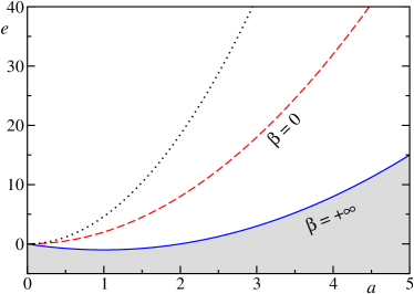
Figure 1: Equilibrium phase diagram in the plane $(a=A/N,e=E/N)$ for the DNLSE as obtained in Rasmussen et al. (2000). The ground state $(\beta=\infty)$ is identified by the curve $e=a^{2}-2a$: the grey area below this curve is inaccessible. The infinite temperature line, $\beta=0$, which corresponds to the parabola $e=2a^{2}$, is the border of the region where ensembles are equivalent, and represents also the transition line for the localization phase transition in the $N\rightarrow\infty$ limit. For finite $N$, the localization transition occurs above the $\beta=0$ line: black dotted curve represents the transition line for $N=100$.

II The Discrete Non-Linear Schrödinger equation: generalities

The DNLSE is a one-dimensional model of a scalar complex field $z_{j}$ on a lattice made of $N$ sites with periodic boundary conditions , whose Hamiltonian reads

$$\mathcal{H}=\sum_{j=1}^{N}(z_{j}^{*}z_{j+1}+z_{j}z^{*}_{j+1})+\sum_{j=1}^{N}|z_{j}|^{4}\,.$$ (1)

The corresponding Hamiltonian dynamics is expressed by the equations of motion

$$i\dot{z_{j}}=-\frac{\partial\mathcal{H}}{\partial z_{j}^{*}}=-(z_{j+1}+z_{j-1})-2|z_{j}|^{2}z_{j}\,.$$ (2)

It is crucial to note that these equations of motion conserve not only the total energy $\mathcal{H}$, but, due to the ‘quantum’ origin of the problem, also the squared norm of the “wave-function”, that is

$$\mathcal{A}=\sum_{j=1}^{N}|z_{j}|^{2}\,.$$ (3)

This quantity $\mathcal{A}$ can also be interpreted as the total number of particles present in the system. We attribute to $\mathcal{H}$ and $\mathcal{A}$ the real values $E$ and $A$, respectively.

The phase diagram of this model can be easily characterized by representing the complex field in its polar form $z_{j}=e^{i\phi_{j}}\rho_{j}$, so that (1) can be rewritten as

$$\mathcal{H}=2\sum_{j=1}^{N}\rho_{j}\rho_{j+1}\cos(\phi_{j+1}-\phi_{j})+\sum_{j=1}^{N}\rho_{j}^{4}.$$ (4)

It is straightforward to realize that the ground state of this Hamiltonian is obtained when $\cos(\phi_{j+1}-\phi_{j})=-1$ for all $j$, and $\rho_{j}=\rho$, independently of the site index $j$. In terms of the energy and mass densities $e=E/N$ and $a=A/N$, the ground state is identified by the condition $e=-2\,a+a^{2}$, since one has $\rho^{2}=a$. This line is shown in Fig. 1 and in a thermodynamic interpretation it corresponds to the condition $\beta=1/T=+\infty$. Note that the region below this line is not physically accessible. The other important line characterizing the phase diagram corresponds to infinite temperature, i.e. $\beta=0$. One can argue that in this case the angular variables $\{\phi_{j}\}_{j=1,\ldots,N}$ have to behave as independent identically distributed (i.i.d) random variables, so that the first addendum in the r.h.s. of Eq. (4) is proportional to $\sqrt{N}$, while the second one is proportional to $N$. Therefore the contribution of the bilinear terms to the total energy is subleading and we will neglect it in our calculation of the partition function, done in the spirit of a large-$N$ estimate. At high temperatures the subleading nature of the bilinear terms, which should give a term proportional to $a$, is confirmed by the exact analytical result of Rasmussen et al. (2000). In Rasmussen et al. (2000) such bilinear terms are taken into account and, despite this, the $\beta=0$ line is still identified by the condition $e=2\,a^{2}$ (see Fig. 1): that is, there is no term linear in $a$.

Due to the presence of two conserved quantities, the deterministic dynamics of this model exhibits quite peculiar features. In the region sandwitched between the zero temperature line and the infinite temperature one, any initial condition relaxes to a uniform equilibrium state displaying equipartition. Conversely, above the ($\beta=0$)-line the dynamics on any finite lattice is characterized by the birth and death of long-living localized nonlinear excitations, called breathers (e.g. see Trombettoni and Smerzi (2001); Franzosi et al. (2011)). In a stochastic version of the dynamics Iubini et al. (2014, 2017a) still conserving both $E$ and $A$, the evolution in the region above the ($\beta=0$)-line has been found to lead to a coarsening process eventually yielding a state where a giant breather confined in a finite lattice region collects a finite fraction of the total energy and norm (number of particles). In particular, the condensate “mass” has been found to increase in time $t$ as $t^{1/3}$. One cannot exclude that also the deterministic dynamics in the localized phase might eventually evolve to this single-breather state, even though it has never been observed even in relatively small lattices.

Finding an interpretation of this scenario is related to the understanding of the thermodynamics of the DNLSE model. Various attempts have been made to study its equilibrium properties in the presence of a localized wave-function  Rasmussen et al. (2000); Barré and Mangeolle (2018). The reason why a study of the thermodynamics deep in the localized phase has been (to some extent) so far elusive is that the ($\beta=0$)-line, where condensation takes place, corresponds also to the breakdown of the equivalence between statistical ensembles, as we are going to show in Sec. III.2. In this respect, it is worth quoting a series of recent papers, focused on the regression dynamics of large anomalous fluctuations, where it has been argued that isolated anomalous fluctuations should be somehow related to ensemble inequivalence Corberi (2015, 2017); Corberi et al. (2019). Nevertheless, we need to stress that our present work demonstrates in a clear and transparent manner that the physics of the localized phase in the DNLSE can be described consistently only in the microcanonical ensemble.

In fact, the main goal of this paper is the computation of the microcanonical entropy of the DNLSE Hamiltonian (1) for fixed values of $E$ and $A$ close to the ($\beta=0$)-line, shown in Fig. 1. In general, the microcanonical entropy is defined as

$${\color[rgb]{0,0,0}S_{N}(A,E)=\log~{}\Omega_{N}^{O}(A,E)},$$ (5)

where the Boltzmann constant $k_{B}$ is set to unit and $\Omega_{N}^{O}(A,E)$ is the microcanonical partition function:

$${\color[rgb]{0,0,0}\Omega_{N}^{O}(A,E)}=\int\prod_{j=1}^{N}~{}d\mu(z_{j})~{}\delta\left(A-\sum_{j=1}^{N}|z_{j}|^{2}\right)~{}\delta\left(E-\left[\sum_{j=1}^{N}(z_{j}^{*}z_{j+1}+z_{j}z^{*}_{j+1})+\sum_{j=1}^{N}|z_{j}|^{4}\right]\right).$$ (6)

Here $d\mu(z_{j})$ is a shorthand notation for $d[\Re(z_{j})]\,d[\Im(z_{j})]$.

Since the main interesting features of the DNLSE model occur in the vicinity of the ($\beta=0$)-line, for large values of $N$, as discussed above, the contribution to the total energy $E$ of the bi-linear hopping term in Eq. (1) can be neglected with respect to the local nonlinear term. Accordingly, close to $\beta=0$ the microcanonical partition function can be approximated as follows:

$${\color[rgb]{0,0,0}\Omega_{N}(A,E)}=$$

$$\int\prod_{i=1}^{N}~{}d\mu(z_{j})~{}\delta\left(A-\sum_{j=1}^{N}|z_{j}|^{2}\right)~{}\delta\left(E-\sum_{j=1}^{N}|z_{j}|^{4}\right).$$ (7)

We want to remark that a similar microcanonical partition function with two constraints was also studied Szavits-Nossan et al. (2014a, b, 2016) in the context of generalised mass transport models on a lattice Majumdar et al. (2005); Evans et al. (2006); Evans and Hanney (2005); Majumdar (2010).

III The microcanonical partition function

In this Section we present the explicit computation of the microcanonical partition function $\Omega_{N}(A,E)$ and, in particular, its large deviation properties in the limit of large $N$.

III.1 From statistical mechanics to large deviations

In order to compute ${\color[rgb]{0,0,0}\Omega_{N}(A,E)}$ it is convenient to express the variables in their polar form $z_{j}=\rho_{j}e^{i\phi_{j}}$, thus making straightforward the integration over the angular coordinates $\phi_{i}$:

$${\color[rgb]{0,0,0}\Omega_{N}(A,E)}=$$

$$(2\pi)^{N}\int_{0}^{\infty}\left[\prod_{j=1}^{N}d\rho_{j}~{}\rho_{j}\right]~{}\delta\left(A-\sum_{j=1}^{N}\rho_{j}^{2}\right)~{}\delta\left(E-\sum_{j=1}^{N}\rho_{j}^{4}\right).$$ (8)

The effective strategy for proceeding in this analytic calculation amounts to releasing the conservation constraint on $A$ by means of a Laplace transform:

$$\tilde{\Omega}_{N}(\lambda,E)=\int_{0}^{\infty}dA~{}e^{-\lambda A}~{}{\color[rgb]{0,0,0}\Omega_{N}(A,E)}=$$

$$(2\pi)^{N}\int_{0}^{\infty}~{}\left[\prod_{j=1}^{N}d\rho_{j}~{}\rho_{j}\right]~{}e^{-\lambda\sum_{j=1}^{N}\rho_{j}^{2}}~{}~{}\delta\left(E-\sum_{j=1}^{N}\rho_{j}^{4}\right).$$ (9)

From Eq. (9) the partition function at fixed $A$ can be obtained by a simple inversion of the Laplace transform:

$$\Omega_{N}(A,E)=\frac{1}{2\pi i}\int_{\lambda_{0}-i\infty}^{\lambda_{0}+i\infty}d\lambda~{}e^{\lambda A}~{}\tilde{\Omega}_{N}(\lambda,E),$$ (10)

where integration goes over a vertical Bromwich contour in the complex $\lambda$ plane, crossing the real $\lambda$ axis at a $\lambda_{0}$ which can be chosen to the right of all singularities of the integrand. But, for the moment, let us move forward to the calculation of $\tilde{\Omega}_{N}(\lambda,E)$. By introducing the change of variables $\rho_{j}^{4}=\varepsilon_{j}$ in Eq. (9), it is useful to re-write $\tilde{\Omega}_{N}(\lambda,E)$ as

$$\tilde{\Omega}_{N}(\lambda,E)=$$

$$\left(\frac{\pi}{2}\right)^{N}~{}\int_{0}^{\infty}~{}\prod_{j=1}^{N}\frac{d\varepsilon_{j}}{\sqrt{\varepsilon_{j}}}~{}e^{-\lambda\sum_{j=1}^{N}\sqrt{\varepsilon_{j}}}~{}\delta\left(E-\sum_{j=1}^{N}\varepsilon_{j}\right).$$ (11)

We can introduce the normalized probability distribution function (PDF)

$$f_{\lambda}(\varepsilon)=\Theta(\varepsilon)~{}\frac{\lambda}{2}\frac{1}{\sqrt{\varepsilon}}\exp\left(-\lambda\sqrt{\varepsilon}\right),$$ (12)

where $\Theta(\varepsilon)$ is the Heavyside distribution, and rewrite

$$\tilde{\Omega}_{N}(\lambda,E)=\left(\frac{\pi}{\lambda}\right)^{N}~{}\mathcal{Z}_{N}(\lambda,E)$$ (13)

with

$$\mathcal{Z}_{N}(\lambda,E)=\int_{0}^{\infty}~{}\prod_{j=1}^{N}~{}d\varepsilon_{j}~{}f_{\lambda}(\varepsilon_{j})~{}\delta\left(E-\sum_{j=1}^{N}\varepsilon_{j}\right),$$ (14)

In this form, $\mathcal{Z}_{N}(\lambda,E)$ can be interpreted as the probability distribution of the sum of $N$ i.i.d. random variables $\varepsilon_{j}$, each drawn from the PDF $f_{\lambda}(\varepsilon_{j})$. Note that $\lambda$ appears only as a parameter in the PDF $f_{\lambda}(\varepsilon_{j})$ in Eq. (12).

It is well known from the theory of large deviations Majumdar et al. (2005); Evans et al. (2006); Majumdar (2010) that the global constraint on the sum of the variables yields a condensation phenomenon when the individual probability distribution is fat-tailed, i.e., when it fulfills the following bounds for large $\varepsilon$

$$\exp(-\varepsilon)<{\color[rgb]{0,0,0}f_{\lambda}(\varepsilon)}<\frac{1}{\varepsilon^{2}}\,,$$ (15)

which is exactly the case of Eq. (12). More precisely, when the sum of these i.i.d. random variables (in our case the total energy $E$) overtakes a threshold value (that in our case we denote $E_{\text{th}}$) one observes a crossover from a “fluid phase”, where the sum is democratically shared among all variables (i.e. energy is equally distributed at each lattice position for $E<E_{\text{th}}$) to a “condensed phase”, where the behaviour of $\mathcal{Z}_{N}(\lambda,E)$ in (14) is dominated by the probability distribution $f_{\lambda}(\varepsilon_{i})$ of a single variable (i.e., a macroscopic fraction of the total energy localizes at some lattice site for $E>E_{\text{th}}$). Thus this ‘condensed’ phase precisely corresponds to the ‘localised’ phase in the DNLSE model. The value of $E_{\text{th}}$ is known to be equal to the average total energy, i.e.,

$$E_{\text{th}}=N\,\langle\varepsilon\rangle\,,$$ (16)

where the average $\langle\,\,\,\rangle$ is over the probability distribution $f_{\lambda}(\varepsilon)$ Majumdar (2010). Making use of Eq. (12) one obtains

$$\langle\varepsilon\rangle = \frac{2}{\lambda^{2}}$$

$$\langle\varepsilon^{2}\rangle = \frac{24}{\lambda^{4}}$$

$$\sigma^{2} = \langle\varepsilon^{2}\rangle-\langle\varepsilon\rangle^{2}=\frac{20}{\lambda^{4}}$$ (17)

These results will be used also in the following sections. We anticipate here that the explicit computation of the microcanocal partition function yields $\lambda=1/a$ (see Eq.(51) ) so that we can write $E_{\text{th}}=N\,\langle\varepsilon\rangle=2\,a^{2}\,N$. In the large $N$ limit, this equation amounts to the condition $e=2a^{2}$, i.e. the threshold energy is located exactly at the ($\beta=0$)-line drawn in Fig. 1.

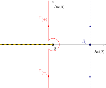
Figure 2: Analytic structure of the function $z(\beta,\lambda)$ (see Eqs. (18),(19)) in the complex $\beta$ plane. Slanted dashed band: branch cut on the negative real semiaxis. Dashed vertical (blue) line: Bromwich contour for the calculation of the partition function $\mathcal{Z}(\lambda,E)$ when $E<E_{\text{th}}$, with $\beta_{0}$ indicating the location of the saddle-point. Continuous (red) line: Bromwich contour to compute ${\color[rgb]{0,0,0}\mathcal{Z}(\lambda,E)}$ when $E>E_{\text{th}}$. The critical energy $E_{\text{th}}\equiv E_{\text{th}}(A)$, where the equivalence between ensembles breaks down, depends on the norm $A$. $\Gamma_{(+)}$ and $\Gamma_{(-)}$ are labels for contour pieces in the positive and negative imaginary semiplanes.

III.2 Analytic properties of the partition function

Before entering the main steps the microcanonical partition function calculation, let us point out that this procedure is very similar to the one employed in Gradenigo and Majumdar (2019) for a model of run-and-tumble particles.

Summarizing, the main steps of the calculation are the followings. We start from the partition function $\mathcal{Z}_{N}(\lambda,E)$ defined in Eq. (14) and we first perform its Laplace transform with respect to $E$, by introducing its conjugate variable $\beta$, which is in general a complex number, i.e. $\beta\in\mathbb{C}$:

$$\tilde{\mathcal{Z}}_{N}(\lambda,\beta)=\int_{0}^{\infty}dE~{}e^{-\beta E}~{}\mathcal{Z}_{N}(\lambda,E)$$

$$=\int_{0}^{\infty}~{}d\varepsilon_{1}\ldots d\varepsilon_{N}~{}e^{-\beta\sum_{j=1}^{N}\varepsilon_{j}}~{}\prod_{j=1}^{N}f_{\lambda}(\varepsilon_{j})$$

$$=\left[\int_{0}^{\infty}d\varepsilon~{}e^{-\beta\varepsilon}~{}f_{\lambda}(\varepsilon)\right]^{N}=\exp\left\{N\log[z(\lambda,\beta)]\right\},$$ (18)

where

$$z(\lambda,\beta)=\int_{0}^{\infty}d\varepsilon~{}e^{-\beta\varepsilon}~{}f_{\lambda}(\varepsilon)$$

$$=\sqrt{\pi}\frac{\lambda}{2\sqrt{\beta}}~{}\exp\left(\frac{\lambda^{2}}{4\beta}\right)~{}\text{Erfc}\left(\frac{\lambda}{2\sqrt{\beta}}\right),$$ (19)

and

$$\text{Erfc}\left(\frac{\lambda}{2\sqrt{\beta}}\right)=\frac{2}{\sqrt{\pi}}\int_{\lambda/(2\sqrt{\beta})}^{\infty}~{}e^{-t^{2}}~{}dt,$$ (20)

is the complementary error function defined in the complex $\beta$ plane, with a branch-cut on the negative real semiaxis (see Fig.2). The original microcanonical partition function $\mathcal{Z}_{N}(\lambda,E)$ can be then recovered by computing the inverse Laplace transform of $\tilde{\mathcal{Z}}_{N}(\lambda,\beta)$:

$$\mathcal{Z}_{N}(\lambda,E)=\int_{\beta_{0}-i\infty}^{\beta_{0}+i\infty}d\beta~{}\exp\left\{N\left(\beta e+\log[z(\lambda,\beta)]\right)\right\}\,.$$ (21)

For large $N$, the integral in Eq. (21) can be evaluated using a saddle-point approximation, where $\beta_{0}$ is the real positive solution of the following equation:

$$e=\frac{E}{N}=-\frac{1}{z(\lambda,\beta)}\frac{\partial z(\lambda,\beta)}{\partial\beta}\,,$$ (22)

If such a real positive value $\beta_{0}$ exists, it can be physically interpreted as an inverse temperature and one could finally write

$$\mathcal{Z}_{N}(\lambda,E)~{}\approx~{}e^{\beta_{0}E+N\log[z(\lambda,\beta_{0})]}.$$ (23)

What happens in the DNLSE model is that Eq. (22) for $E<E_{\text{th}}$ admits a unique real positive solution and the integration contour is shown by the dashed (blue) line in Fig.2. Conversely, for $E>E_{\text{th}}$ a real positive solution of Eq. (22) does not exist, due to the presence of the branch-cut of $z(\lambda,\beta)$ on the real negative semiaxis. Accordingly, the equivalence between the canonical and the microcanonical ensemble cannot hold for $E>E_{\text{th}}$. Anyway, the calculation of $\mathcal{Z}_{N}(\lambda,E)$ can be performed by considering the analytic continuation of $z(\lambda,\beta)$ in the complex $\beta$ plane and deforming the integration contour as shown by the continuous (red) line in Fig. 2. Following similar large-deviation calculations, contained in a series of papers  Majumdar et al. (2005); Evans et al. (2006); Szavits-Nossan et al. (2014a); Gradenigo and Majumdar (2019), one can recover $\mathcal{Z}_{N}(\lambda,E)$ for $E>E_{\text{th}}$ making use of suitable expansions of $z(\lambda,\beta)$ around the origin $\beta=0$. Consider evaluating $\mathcal{Z}_{N}(\lambda,E)$ for a given fixed scale $\Delta E=E-E_{\text{th}}\sim N^{\gamma}$ of the excess energy where the exponent $\gamma$ can be chosen depending on which scale we want to probe the system. One then needs to retain the leading terms only up to a given scale in the expansion of $z(\lambda,\beta)$. For instance, as explicitly reported in  Gradenigo and Majumdar (2019), one can evaluate $\mathcal{Z}_{N}(\lambda,E)$ at the energy scale $\Delta E=E-E_{\text{th}}\sim N^{1/2}$ (Gaussian regime) by expanding $z(\lambda,\beta)$ around $\beta=0$ up to the order $\beta\sim N^{-1/2}$, thus obtaining the almost trivial result

$$\mathcal{Z}_{N}(\lambda,E)=\frac{1}{\sigma\sqrt{2\pi N}}\exp\left[-\frac{(E-E_{\text{th}})^{2}}{2\sigma^{2}N}\right]\,,$$ (24)

which is a straightforward consequence of the Central Limit Theorem, the dependence on $\lambda$ coming through $\sigma$ (see Eq. (17)). On the other hand, if one aims at evaluating $\mathcal{Z}_{N}(\lambda,E)$ at the order $\Delta E=E-E_{\text{th}}\sim N$, which in Gradenigo and Majumdar (2019) is called the extreme large-deviation regime, one has to retain consistently terms of the expansion of $z(\lambda,\beta)$ up to the order $\beta\sim 1/N$. In this case one obtains:

$$\mathcal{Z}_{N}(\lambda,E)\sim\exp\left(-\sqrt{E-E_{\text{th}}}\right).$$ (25)

As discussed in Sec. IV.2, the Gaussian regime and the extreme large-deviation regime correspond to a delocalized and to a localized phase, respectively. Therefore, in order to understand whether the crossover between these two phases occurs as a real thermodynamic phase transition, one has to identify an intermediate matching regime, which can be heuristically singled out by the following condition

$$\frac{(E-E_{\text{th}})^{2}}{2\sigma^{2}N}\approx\sqrt{E-E_{\text{th}}}\,,$$ (26)

allowing to recognize the intermediate scale

$$E-E_{\text{th}}\sim N^{2/3}.$$ (27)

III.3 Matching regime: the non-analytic contribution

The main result of this section is the proof that in the matching regime the partition function splits into the sum of a Gaussian contribution and of a non-analytic one, denoted by $\mathcal{C}(\lambda,\zeta)$:

$$\mathcal{Z}_{N}(\lambda,E)=\frac{1}{\sigma\sqrt{2\pi N}}\exp{\left(-N^{1/3}\frac{\zeta^{2}}{2\sigma^{2}}\right)}+{\color[rgb]{0,0,0}\mathcal{C}(\lambda,\zeta)}\,,$$ (28)

where

$$\zeta=\frac{E-E_{\text{th}}}{N^{2/3}}$$ (29)

is the scaling variable suggested by the matching condition in Eq. (26). The first term on the r.h.s. of Eq. (28) comes from the straight part of the deformed contour in Fig. 2 (continuous red line), while the non-analytic contribution, $\mathcal{C}(\lambda,\zeta)$, is due to the non-analyticity at the branch-cut along the negative real axis.

Since for $E>E_{\text{th}}$ the saddle-point condition in Eq. (22) has no real solution, we have to consider the analytic prolongation of $z(\lambda,\beta)$ in the complex $\beta$ plane and to evaluate its expansion around the origin $\beta=0$ separately along the upper and lower branch cut, i.e. for $\Re(\beta)<0$:

$$\lim_{\delta\rightarrow 0}z(\lambda,\beta+i\delta) = z(\lambda,\beta+i0^{+})$$

$$\lim_{\delta\rightarrow 0}z(\lambda,\beta-i\delta) = z(\lambda,\beta+i0^{-}).$$ (30)

The expansion around $\beta=0$ yields the expressions

$$z(\lambda,\beta+i0^{+})=$$

$$1-\langle\varepsilon\rangle\beta+\frac{1}{2}\langle\varepsilon^{2}\rangle\beta^{2}+\ldots+\sqrt{\frac{2\pi}{\langle\varepsilon\rangle\beta}}~{}\exp\left(\frac{1}{2\langle\varepsilon\rangle\beta}\right)$$

$$z(\lambda,\beta+i0^{-})=1-\langle\varepsilon\rangle\beta+\frac{1}{2}\langle\varepsilon^{2}\rangle\beta^{2}+\ldots,$$ (31)

where $\langle\varepsilon\rangle$ and $\langle\varepsilon^{2}\rangle$ are defined in Eq. (17) in terms of $\lambda$. Accordingly, the expansion of the local free energy reads:

$$\log[z(\lambda,\beta+i0^{+})]=$$

$$-\langle\varepsilon\rangle~{}\beta+\frac{1}{2}\sigma^{2}~{}\beta^{2}+\mathcal{O}(\beta^{3})+\ldots+\sqrt{\frac{2\pi}{\langle\varepsilon\rangle\beta}}~{}\exp\left(\frac{1}{2\langle\varepsilon\rangle\beta}\right)$$

$$\log[z(\lambda,\beta+i0^{-})]=-\langle\varepsilon\rangle~{}\beta+\frac{1}{2}\sigma^{2}~{}\beta^{2}+\mathcal{O}(\beta^{3}),$$ (32)

where $\sigma$ is defined in Eq. (17) in terms of $\lambda$. The non-analiticity of $z(\lambda,\beta)$ at the cut, clearly expressed by the difference between the first and the second line of Eq. (32), suggests to evaluate the contour integral which defines $\mathcal{Z}_{N}(\lambda,E)$ [see Eq. (21)] by splitting it in two parts:

$$\mathcal{Z}_{N}(\lambda,E)=\mathcal{I}^{(+)}(\lambda,E)+\mathcal{I}^{(-)}(\lambda,E)\,.$$ (33)

The two terms $\mathcal{I}^{(+)}(\lambda,E)$ and $\mathcal{I}^{(-)}(\lambda,E)$ in the equation above can be evaluated by introducing explicitly the expansions of Eq. (32) into the integral of Eq. (21). Recalling then that $E_{\text{th}}=N\langle\varepsilon\rangle$ one obtains

$$\mathcal{I}^{(+)}(\lambda,E) = \int_{\Gamma^{(+)}}\frac{d\beta}{2\pi i}~{}\exp\left\{\beta(E-E_{\text{th}})+\frac{N}{2}\sigma^{2}\beta^{2}+N\mathcal{O}(\beta^{3})+N\sqrt{\frac{2\pi}{\langle\varepsilon\rangle\beta}}~{}\exp\left(\frac{1}{2\langle\varepsilon\rangle\beta}\right)\right\}$$

$$\mathcal{I}^{(-)}(\lambda,E) = \int_{\Gamma^{(-)}}\frac{d\beta}{2\pi i}~{}\exp\left\{\beta(E-E_{\text{th}})+\frac{N}{2}\sigma^{2}\beta^{2}+N\mathcal{O}(\beta^{3})\right\}\,,$$

where the integration paths $\Gamma^{(+)}$ and $\Gamma^{(-)}$ are those shown in Fig.2. A better interpretation of this result can be obtained by introducing the scaling variable $\zeta$ defined in Eq. (29):

$$\mathcal{I}^{(+)}(\lambda,\zeta) = \int_{\Gamma^{(+)}}\frac{d\beta}{2\pi i}~{}\exp\left\{\beta~{}\zeta~{}N^{2/3}+\frac{N}{2}\sigma^{2}\beta^{2}+N\mathcal{O}(\beta^{3})+N\sqrt{\frac{2\pi}{\langle\varepsilon\rangle\beta}}~{}\exp\left(\frac{1}{2\langle\varepsilon\rangle\beta}\right)\right\}$$

$$\mathcal{I}^{(-)}(\lambda,\zeta) = \int_{\Gamma^{(-)}}\frac{d\beta}{2\pi i}~{}\exp\left\{\beta~{}\zeta~{}N^{2/3}+\frac{N}{2}\sigma^{2}\beta^{2}+N\mathcal{O}(\beta^{3})\right\}.$$

Since $\Re(\beta)<0$, for asymptotically small values of $\beta$ one has that the non-analytic term $\exp[1/(2\langle\varepsilon\rangle\beta)]$ is exponentially small and, at leading order in $N$, we can write

$$\exp\left[N\sqrt{\frac{2\pi}{\langle\varepsilon\rangle\beta}}~{}\exp\left(\frac{1}{2\langle\varepsilon\rangle\beta}\right)\right]\approx 1+N\sqrt{\frac{2\pi}{\langle\varepsilon\rangle\beta}}~{}\exp\left(\frac{1}{2\langle\varepsilon\rangle\beta}\right).$$ (36)

By substituting the above expansion into the integral $\mathcal{I}^{(+)}(\lambda,\zeta)$ we obtain

$$\mathcal{I}^{(+)}(\lambda,\zeta)=\int_{\Gamma^{(+)}}\frac{d\beta}{2\pi i}~{}e^{\beta\zeta N^{2/3}+\frac{N}{2}\sigma^{2}\beta^{2}+N\mathcal{O}(\beta^{3})}+$$

$$+N\sqrt{\frac{2\pi}{\langle\varepsilon\rangle\beta}}\int_{\Gamma^{(+)}}\frac{d\beta}{2\pi i}~{}e^{\beta\zeta N^{2/3}+\frac{N}{2}\sigma^{2}\beta^{2}+N\mathcal{O}(\beta^{3})+\frac{1}{2\langle\varepsilon\rangle\beta}}.$$ (37)

A more refined way to implement the matching argument at the end of III.2 is to set the scale of the (complex) neighbourhood of $\beta=0$ in such a way that the analytic and the non-analytic terms in the expansion of $\log[z(\lambda,\beta)]$ are of the same order in $N$: in fact, these terms account respectively for the homogeneous and the localized phase.

Since we want to evaluate the integrals in Eq. (37) by means of a saddle-point approximation, we have to chose the proper scale of $\beta$. This task can be accomplished by first introducing the change of variable to $\hat{\beta}=N^{\gamma}\beta$ in the integral of Eq. (37) and then by fixing the value of the exponent $\gamma$ in such a way to single out the same power of $N$ in each term of the following expression:

$$\hat{\beta}\zeta~{}N^{2/3-\gamma}+\frac{N^{1-2\gamma}}{2}\sigma^{2}\hat{\beta}^{2}+\frac{N^{\gamma}}{2\langle\varepsilon\rangle\hat{\beta}}.$$ (38)

This is condition holds if there is a value of $\gamma$ such that

$$2/3-\gamma=1-2\gamma=\gamma,$$ (39)

thus yielding $\gamma=1/3$. The integrals in Eq. (37) can be rewritten in the following form

$$\mathcal{I}^{(+)}(\lambda,\zeta)=\frac{1}{N^{1/3}}\int_{\Gamma^{(+)}}\frac{d\beta}{2\pi i}~{}e^{N^{1/3}[\beta\zeta+\frac{1}{2}\sigma^{2}\beta^{2}]}+$$

$$N\sqrt{\frac{2\pi}{\langle\varepsilon\rangle}}\int_{\Gamma^{(+)}}\frac{d\beta}{2\pi i}~{}\frac{1}{\sqrt{N^{1/3}\beta}}e^{N^{1/3}\left[\beta\zeta+\frac{1}{2}\sigma^{2}\beta^{2}+\frac{1}{2\langle\varepsilon\rangle\beta}\right]},$$ (40)

where the integration variable $\beta$ has been rescaled by a factor $N^{1/3}$. Similarly, the integral in the negative imaginary semiplane turns to the expression

$$\mathcal{I}^{(-)}(\lambda,\zeta)=\frac{1}{N^{1/3}}\int_{\Gamma^{(-)}}\frac{d\beta}{2\pi i}~{}e^{N^{1/3}[\beta\zeta+\frac{1}{2}\sigma^{2}\beta^{2}]}\,.$$ (41)

By summing these two contributions one finally obtains the partition function $\mathcal{Z}_{N}(\lambda,E)$. It is convenient to change the variable $E$ to the scaled variable $\zeta=(E-E_{\rm th})/N^{2/3}$ in $\mathcal{Z}_{N}(\lambda,E)$, and with a slight abuse of notation, we will continue to denote the partition function as $\mathcal{Z}_{N}(\lambda,\zeta)$. We then obtain

$$\mathcal{Z}_{N}(\lambda,\zeta) = \mathcal{I}^{(+)}(\lambda,\zeta)+\mathcal{I}^{(-)}(\lambda,\zeta)=$$ (42)

$$= \frac{1}{N^{1/3}}\int_{-i\infty}^{i\infty}\frac{d\beta}{2\pi i}~{}e^{N^{1/3}[\beta\zeta+\frac{1}{2}\sigma^{2}\beta^{2}]}+{\color[rgb]{0,0,0}\mathcal{C}(\lambda,\zeta)},$$

$$= \frac{1}{\sigma\sqrt{2\pi N}}e^{-N^{1/3}\frac{\zeta^{2}}{2\sigma^{2}}}+{\color[rgb]{0,0,0}\mathcal{C}(\lambda,\zeta)}$$

where the non-analytic contribution to the partition function is

$${\color[rgb]{0,0,0}\mathcal{C}(\lambda,\zeta)}=N\sqrt{\frac{2\pi}{\langle\varepsilon\rangle}}\int_{\Gamma^{(+)}}\frac{d\beta}{2\pi i}~{}\frac{1}{\sqrt{N^{1/3}\beta}}e^{N^{1/3}F_{\zeta}(\lambda,\beta)}\,,$$ (43)

with

$$F_{\zeta}(\lambda,\beta)=\beta\zeta+\frac{1}{2}\sigma^{2}\beta^{2}+\frac{1}{2\langle\varepsilon\rangle\beta}\,.$$ (44)

Note that the dependence of $F_{\zeta}(\lambda,\beta)$ on $\lambda$ comes from the fact that both $\langle\varepsilon\rangle$ and $\sigma^{2}$ appearing in Eq. (44) are functions of $\lambda$ [see Eq. (17)].

The decomposition of the partition function in the matching regime as the sum of two contributions is the main result of this section. It remains to perform the explicit calculation of the integral ${\color[rgb]{0,0,0}\mathcal{C}(\lambda,\zeta)}$.

This task can be accomplished by following the same procedure reported in Gradenigo and Majumdar (2019): the key point of the calculation amounts to finding the solution $\beta^{*}(\zeta)$ of the saddle-point equation:

$$\frac{\partial F_{\zeta}(\lambda,\beta)}{\partial\beta}=0\,.$$ (45)

Details of the calculations are illustrated in Appendices VII.1 and VII.2. Here we just provide the final result:

$$\int_{\Gamma^{(+)}}\frac{d\beta}{2\pi i}~{}\frac{1}{\sqrt{N^{1/3}\beta}}~{}e^{N^{1/3}F_{\zeta}(\lambda,\beta)}\approx e^{-N^{1/3}\chi(\zeta)}\,,$$ (46)

where the explicit form of $\chi(\zeta)$ is discussed in Appendix VII.1. Its asymptotic behaviours are:

$$\chi(\zeta)=\begin{cases}\frac{3}{2}\left(\frac{\sigma}{\langle\varepsilon\rangle}\right)^{2/3}\qquad\qquad\qquad\qquad\zeta\rightarrow\zeta_{l}\\ \\ \sqrt{\frac{2}{\langle\varepsilon\rangle}}\sqrt{\zeta}-\frac{\sigma^{2}}{4\langle\varepsilon\rangle}\frac{1}{\zeta}+\mathcal{O}\left(\frac{1}{\zeta^{5/2}}\right),\quad\zeta\gg 1\end{cases},$$ (47)

where $\zeta_{l}$ is the spinodal point for the localized phase, that is the smallest value of $\zeta$ for which the saddle-point equation Eq. (45) admits a real solution, namely

$$\zeta_{l}=\frac{3}{2}~{}\left(\frac{\sigma^{4}}{\langle\varepsilon\rangle}\right)^{1/3}.$$ (48)

IV The first-order phase transition from a thermalized phase to localization

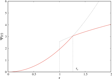
Figure 3: Continuous (red) line: behaviour of the sub-leading contribution $\Psi(r)$ (see Eq. (54)) to the microcanonical entropy as a function of the adimensional variable $r=\zeta/\zeta_{l}$, with $\zeta_{l}$ defined in Eq. (48). Making use of this rescaled variable $r$, the spinodal point is located at $r=1$. The first order transition is located at $r_{c}=\zeta_{c}/\zeta_{l}\approx 2^{1/3}$, where $d\Psi(r)/dr$ is discontinuous: the value of $\zeta_{c}$ is determined by the argument in Appendix VII.3. The dashed lines draw the function $\chi(r)$ (see Eqs. (46),(47)) for $r<r_{c}$ and $r^{2}/(2\sigma^{2})$ for $r>r_{c}$.

IV.1 The microcanonical entropy in the matching regime

We are now in the position of retrieving the microcanonical partition function by computing the inverse Laplace transform of Eq. (10):

$${\color[rgb]{0,0,0}\Omega_{N}(A,E)}=\frac{1}{2\pi i}\int_{\lambda_{0}-i\infty}^{\lambda_{0}+i\infty}d\lambda~{}e^{\lambda A}~{}\tilde{\Omega}_{N}(\lambda,E)$$

$$=\frac{e^{N\log(\pi)}}{2\pi i}\int_{\lambda_{0}-i\infty}^{\lambda_{0}+i\infty}d\lambda~{}e^{N[a\lambda-\log(\lambda)]}~{}\mathcal{Z}_{N}(\lambda,E),$$ (49)

where the final expression on the r.h.s. of Eq. (49) is obtained thanks to Eq. (13). In order to point out the presence of a phase transition, we are interested to obtain an analytic estimate of ${\color[rgb]{0,0,0}\Omega_{N}(A,\zeta)}$ in the matching regime, where $\mathcal{Z}_{N}(\lambda,\zeta)$ is given by Eqs. (42) and Eq. (43) and $\zeta=(E-E_{\text{th}})/N^{2/3}\approx\mathcal{O}(1)$:

$${\color[rgb]{0,0,0}\Omega_{N}(A,\zeta)}=$$

$$\frac{e^{N\log(\pi)}}{2\pi i}\int_{\lambda_{0}-i\infty}^{\lambda_{0}+i\infty}d\lambda~{}e^{N[a\lambda-\log(\lambda)]}~{}\left[e^{-N^{1/3}\chi(\zeta)}+e^{-N^{1/3}\zeta^{2}/(2\sigma^{2})}\right].$$ (50)

In the thermodynamic limit, $N\to\infty$, the leading contribution to the integral on the r.h.s. of Eq. (50) is given by the term $N[a\lambda-\log(\lambda)]$, which determines the value of $\lambda_{0}$ as the solution of the saddle-point equation

$$\frac{\partial}{\partial\lambda}[a\lambda-\log(\lambda)]=0\qquad\longrightarrow\qquad\lambda_{0}=1/a\,.$$ (51)

The complete expression of ${\color[rgb]{0,0,0}\Omega_{N}(A,\zeta)}$ is thus obtained by replacing the multiplier $\lambda$ with its actual value $\lambda_{0}=1/a$. Accordingly, in the matching regime the complete partition function reads

$${\color[rgb]{0,0,0}\Omega_{N}(A,\zeta)}~{}\approx~{}e^{N\left[1+\log(\pi a)\right]}~{}\left[e^{-N^{1/3}\chi(\zeta)}+e^{-N^{1/3}\zeta^{2}/(2\sigma^{2})}\right],$$ (52)

where we point out that, by plugging $\lambda=1/a$ into Eq. (17), one has $\sigma^{2}=20\,a^{4}$ and $\langle\varepsilon\rangle=2\,a^{2}$. Note that we need $\langle\varepsilon\rangle$ to evaluate $\chi(\zeta)$ in Eq. (47). This result provides us with the expression for the microcanonical entropy at leading and sub-leading order in the limit of large $N$:

$$S_{N}(A,\zeta)=N\left[1+\log(\pi a)\right]-N^{1/3}\Psi(\zeta),$$ (53)

where

$$\Psi(\zeta)=\text{inf}_{\zeta}\Big{\{}\chi(\zeta),\zeta^{2}/(2\sigma^{2})\Big{\}}\,,$$ (54)

The leading term in $S_{N}(A,\zeta)$ is extensive in $N$ and represents the contribution of the bulk of the system at infinite temperature, i.e. the background entropy,

$$S_{N}^{\text{back}}(a)=N\left[1+\log(\pi a)\right]=Ns^{\text{back}}(a).$$ (55)

Note that this contribution does not depend on $\zeta$, i.e. on the excess energy $\Delta E=E-E_{\text{th}}$ contained in the condensate, which appears exclusively only in the sub-leading term in $\Psi(\zeta)$. Accordingly, we can identify the critical value $\zeta_{c}$ for localization as the one where the sub-leading contribution to the entropy of the localized and that of the delocalized phase have identical magnitude, i.e., by the following matching condition

$$\chi(\zeta_{c})=\zeta_{c}^{2}/(2\sigma^{2})\,.$$ (56)

The function $\Psi(\zeta)$ is shown in Fig.3: more precisely, we have decided to draw it as a function of the rescaled variable $r=\zeta/\zeta_{l}$. From the argument discussed in App. VII.3 we find that the critical value of $r$, which does not depend on the parameters of individual energy distributions on lattice sites, is

$$r_{c}=\frac{\zeta_{c}}{\zeta_{l}}=2^{1/3}.$$ (57)

Since the derivative of $\Psi(\zeta)$ is discontinuous at $\zeta_{c}$, we can conclude that we are facing a first–order phase transition, from a thermalized phase to a localized one.

IV.2 The order parameter: participation ratio

The localization transition can be further characterized by introducing the participation ratio of the energy per site

$$Y_{2}=\left\langle\frac{\sum_{j=1}^{N}\varepsilon_{j}^{2}}{\left(\sum_{j=1}^{N}\varepsilon_{j}\right)^{2}}\right\rangle_{A,E},$$ (58)

as a suitable order parameter, where the angular brackets denote the microcanonical equilibrium average. Indeed, if the total energy $E=eN$ is uniformly distributed over all sites, i.e. $\varepsilon_{j}\sim e$ for each $j$, then the numerator in Eq. (58) scales as $N$ and the denominator scales as $N^{2}$. Consequently $Y_{2}=\mathcal{O}(N^{-1})$. In contrast, when an extensive amount of energy is localized at a single site (i.e. in the presence of a condensate), the numerator scales as $N^{2}$ while the denominator still scales as $N^{2}$. Therefore, $Y_{2}=\mathcal{O}(1)$ in the large $N$ limit. Hence, the quantity $Y_{2}$ is a good observable to detect the localization transition.

For our purposes it is enough to analyze the behavior of $Y_{2}$ in the proximity of the threshold energy, i.e., at $E\sim E_{\text{th}}=N\langle\varepsilon\rangle$ (see Sec. III.1), where, as discussed in the previous section, the transition point is located. In this regime the equilibrium joint probability distribution of local energies has, within the microcanonical ensemble, the following expression

$$P(\varepsilon_{1},\ldots,\varepsilon_{N})=\frac{e^{Ns^{\text{back}}(a)}}{{\color[rgb]{0,0,0}\Omega_{N}(A,E)}}\prod_{j=1}^{N}~{}f_{a}(\varepsilon_{j})~{}\delta\left(E-\sum_{j=1}^{N}\varepsilon_{j}\right)\,,$$ (59)

where

$${\color[rgb]{0,0,0}\Omega_{N}(A,E)}=$$

$$e^{Ns^{\text{back}}(a)}\int_{0}^{\infty}\prod_{j=1}^{N}~{}\left[d\varepsilon_{j}~{}f_{a}(\varepsilon_{j})~{}\right]~{}\delta\left(E-\sum_{j=1}^{N}\varepsilon_{j}\right)$$ (60)

is the microcanonical partition function. In fact, as shown in the previous section [see the saddle-point condition in Eq. (51)], ${\color[rgb]{0,0,0}\Omega_{N}(A,E)}$ in the matching regime can be written as a function of the probability distributions $f_{a}(\varepsilon_{j})$ of i.i.d. energy variables, where the label $\lambda$ appearing in Eq. (12) can be replaced by the label $a$, since by means of the saddle-point condition in Eq. (51) we have fixed $\lambda=1/a$, i.e., the inverse of the solution of the saddle-point condition. By plugging the expression of $P(\varepsilon_{1},\ldots,\varepsilon_{N})$ written in Eq. (59) into the definition of $Y_{2}$ given in Eq. (58), we obtain:

$$Y_{2}(E) =\frac{e^{Ns^{\text{back}}(a)}}{{\color[rgb]{0,0,0}\Omega_{N}(A,E)}}\int_{0}^{\infty}d\varepsilon_{1}\ldots d\varepsilon_{N}~{}\prod_{j=1}^{N}~{}f_{a}(\varepsilon_{j})~{}\frac{\sum_{j=1}^{N}\varepsilon_{j}^{2}}{\left(\sum_{j=1}^{N}\varepsilon_{j}\right)^{2}}~{}\delta\left(E-\sum_{j=1}^{N}\varepsilon_{j}\right)$$

$$=\frac{Ne^{s^{\text{back}}(a)}}{E^{2}}\int_{0}^{\infty}d\varepsilon~{}\varepsilon^{2}~{}f_{a}(\varepsilon)~{}\frac{\left[e^{(N-1)s^{\text{back}}(a)}~{}\int d\varepsilon_{2}\ldots d\varepsilon_{N}\prod_{j=2}^{N}f_{a}(\varepsilon_{j})\delta\left(E-\varepsilon-\sum_{j=2}^{N}\varepsilon_{i}\right)\right]}{{\color[rgb]{0,0,0}\Omega_{N}(A,E)}}$$

$$=\frac{Ne^{s^{\text{back}}(a)}}{E^{2}}\int_{0}^{\infty}d\varepsilon~{}\varepsilon^{2}~{}f_{a}(\varepsilon)~{}\frac{\Omega_{N-1}(A,E-\varepsilon)}{{\color[rgb]{0,0,0}\Omega_{N}(A,E)}}\,,$$ (61)

where the term

$$e^{s^{\text{back}}(a)}f_{a}(\varepsilon)\frac{{\color[rgb]{0,0,0}\Omega_{N-1}(A,E-\varepsilon)}}{{\color[rgb]{0,0,0}\Omega_{N}(A,E)}}\equiv\rho(\varepsilon)$$ (62)

is the normalized marginal distribution of the energy $\varepsilon$ on a single site  . Accordingly, the participation ratio takes the compact form

$$Y_{2}(E) = \frac{N}{E^{2}}\int_{0}^{\infty}d\varepsilon~{}\varepsilon^{2}~{}\rho(\varepsilon)$$ (63)

$$= \frac{N}{E^{2}}~{}\langle\varepsilon^{2}\rangle\,,$$

As a first step in the study of the behavior of the order parameter $Y_{2}$, we observe that the condition $E^{2}\sim N^{2}$ implies that Eq. (63) reads in practice as $Y_{2}(E)\sim\langle\varepsilon^{2}\rangle/N$.

Let us first consider the estimate of $Y_{2}$ in the case when $E<E_{th}$. Since the total energy is below the threshold, $\Omega_{N}(A,E)$ can be safely computed by means of a saddle point approximation, yielding

$$\Omega_{N}(A,E)\approx e^{\beta_{0}E+N\log[z(a,\beta_{0})]}.$$ (64)

It is then crucial the calculation of ${\color[rgb]{0,0,0}\Omega_{N-1}(A,E-\varepsilon)}$ in Eq. (62), which, for large values of $N$, can be approximated in a completely harmless way with ${\color[rgb]{0,0,0}\Omega_{N}(A,E-\varepsilon)}$. Since the value of the energy $\varepsilon$ on a single site can be at most $\varepsilon=E$, we have that the domain of the variable $y=E-\varepsilon$ is $y\in[0,E]$. Hence the integral which defines ${\color[rgb]{0,0,0}\Omega_{N}(A,y=E-\varepsilon)}$ through its inverse Laplace transform can be computed by a saddle-point approximation for all values of $y$, since we always have $y=E-\varepsilon<E_{th}$:

$${\color[rgb]{0,0,0}\Omega_{N}(A,E-\varepsilon)} =\int_{\beta_{0}-i\infty}^{\beta_{0}+i\infty}d\beta~{}e^{\beta(E-\varepsilon)+N\log[z(a,\beta)]}$$

$$\approx e^{\beta_{0}(E-\varepsilon)+N\log[z(a,\beta_{0})]}$$

so that

$$\frac{{\color[rgb]{0,0,0}\Omega_{N-1}(A,E-\varepsilon)}}{{\color[rgb]{0,0,0}\Omega_{N}(A,E)}}=e^{-\beta_{0}\varepsilon}~{}\Longrightarrow~{}\frac{\langle\varepsilon^{2}\rangle}{N}\sim\frac{1}{N}.$$ (66)

Accordingly, for $E<E_{\text{th}}$ the participation ratio vanishes as $1/N$ for large $N$. This confirms that in the thermalized phase close to $E_{\textrm{th}}$ localization of energy is absent, as expected. For $E>E_{\textrm{th}}$ we cannot rely anymore on the saddle-point approximation for $\beta$ to compute the integral in Eq. (66). Still, from the study of ${\color[rgb]{0,0,0}\Omega_{N}(A,E)}$ we known that at the scale $E-E_{\text{th}}\sim N^{1/2}$ the partition function has a Gaussian shape. Therefore, we have that for values of $E$ up to the scale $E-E_{\text{th}}\sim N^{1/2}$ the marginal probability distribution of energy scales as

$${\color[rgb]{0,0,0}\rho(\varepsilon)}\approx f_{a}(\varepsilon)\frac{\exp[-(\Delta E-\varepsilon)^{2}/(2\sigma^{2}N)]}{\exp[-(\Delta E)^{2}/(2\sigma^{2}N)]}\,,$$ (67)

where $\Delta E=E-E_{\text{th}}$. By expanding the square in the exponential in the numerator we obtain a term which simplifies with the denominator and we are left with the expression:

$${\color[rgb]{0,0,0}\rho(\varepsilon)}\approx f_{a}(\varepsilon)~{}\exp\left[-\frac{\varepsilon^{2}}{2\sigma^{2}N}+\frac{\varepsilon\Delta E}{\sigma^{2}N}\right]\,.$$ (68)

Recalling now that $\Delta E\sim\sqrt{N}$, we can estimate the participation ratio by the relation

$$Y_{2}\approx\frac{1}{N}\int_{0}^{\infty}d\varepsilon~{}\varepsilon^{2}~{}f_{a}(\varepsilon)~{}\exp\left[-\frac{\varepsilon^{2}}{2\sigma^{2}N}+\frac{\varepsilon}{\sigma^{2}\sqrt{N}}\right]\,.$$ (69)

In the limit of large $N$ this integral can be approximated as

$$Y_{2}\approx\frac{1}{N}\int_{0}^{\infty}d\varepsilon~{}\varepsilon^{2}~{}f_{a}(\varepsilon)\sim\frac{1}{N}\,,$$ (70)

Therefore for $E>E_{\text{th}}$ and $E-E_{\text{th}}\sim\sqrt{N}$ the participation ratio vanishes asymptotically with $N$. More precisely, the system is still in a delocalized phase, although the decay of $\rho(\varepsilon)$ is not monotonic (see also Fig. 5). With the same argument it can be shown that the same scaling of $Y_{2}$ persists even for $E-E_{\text{th}}\sim N^{2/3}$, i.e. in the matching regime. Altogether, we conclude that the system is delocalized up to $E_{c}$, the critical value of the total energy where the first derivative of the function $\Psi(\zeta)$ in Eq. (53) exhibits the discontinuity. According to Eq. (29), $E_{c}$ reads as:

$$E_{c}=E_{\text{th}}+N^{2/3}\zeta_{c},$$ (71)

where the $\zeta_{c}$ does not depend on $N$ and is determined by the matching condition in Eq. (56), see also Appendix VII.3).

The situation is different for the case of extreme large deviations of the total energy, i.e., following the terminology of Gradenigo and Majumdar (2019), for $E-E_{\text{th}}\sim N$. Also in this case the marginal distribution $\rho(\varepsilon)$ exhibits a bump (see Fig. 5). But in this case the whole $\rho(\varepsilon)$ is dominated in the large $N$ limit by the contribution of the bump, which, for fluctuations of order $\Delta E-\varepsilon\sim N^{1/2}$ around the bump center, reads as

$$\rho(\varepsilon)\approx\rho_{\text{bump}}(\varepsilon)=f_{a}(\varepsilon)~{}\frac{1}{Nf_{a}(\Delta E)}~{}\frac{1}{\sqrt{N}}e^{-(\Delta E-\varepsilon)^{2}/(2\sigma^{2}N)},$$ (72)

where we have used the fact that in the extreme large-deviation regime the whole partition function is identical to $N$ times the distribution of the single variable (see Majumdar et al. (2005); Szavits-Nossan et al. (2014a)), in formulae

$${\color[rgb]{0,0,0}\Omega_{N}(A,E)}\approx N~{}f_{a}(E-E_{\text{th}}).$$ (73)

Since we are interested to the estimate of $\rho_{\text{bump}}(\varepsilon)$ for $\varepsilon\sim\Delta E$, we have $f_{a}(\varepsilon)/f_{a}(\Delta E)=\mathcal{O}(1)$ in the large $N$ limit. Therefore

$$\rho_{\text{bump}}(\varepsilon)~{}\approx~{}\frac{1}{N^{3/2}}~{}\exp[-(\Delta E-\varepsilon)^{2}/(2\sigma^{2}N)]~{}$$

$$\approx~{}\frac{1}{N}~{}\delta(\Delta E-\varepsilon).$$ (74)

By recalling that $\Delta E\sim N$, we finally obtain

$$\int_{0}^{\infty}d\varepsilon~{}\varepsilon^{2}~{}\rho_{\text{bump}}(\varepsilon)=\frac{(\Delta E)^{2}}{N}\sim N,$$ (75)

so that in this limit $Y_{2}$ is finite and independent of $N$. These features signal the presence of the localized phase. We point out that localization of energy is on a single site, as the ratio between the width of the bump, of order $N^{1/2}$, and its position $\Delta E\sim N$, vanishes asymptotically.

Overall, the scenario can be summarized according to the following scheme, where the critical value of the energy $E_{c}$ is the one defined in Eq. (71):

• $E<E_{\text{th}}$: ${\color[rgb]{0,0,0}\rho(\varepsilon)}$ decays monotonically at large $\varepsilon$ and the participation ratio decays asymptotically as

  $$Y_{2}(E)\sim\frac{1}{N}\,.$$ (76)

• $E_{\text{th}}<E<E_{c}$: the decay of ${\color[rgb]{0,0,0}\rho(\varepsilon)}$ at large values of $\varepsilon$ is non monotonic and the formation of a secondary bump can be seen in Fig. 5. This notwithstanding, the participation ratio still vanishes asymptotically as

  $$Y_{2}(E)\sim\frac{1}{N}\,.$$ (77)

  In analogy with recent results on constraint-driven condensation Gradenigo and Bertin (2017), we refer to this intermediate regime as the pseudo-condensate phase.

• $E>E_{c}$: $\rho(\varepsilon)$ has a bump placed at $\varepsilon^{*}={\color[rgb]{0,0,0}(E-E_{th})}$ and the participation ratio goes asymptotically to a value independent on $N$:

  $$Y_{2}(E)=\frac{(E-E_{\text{th}})^{2}}{E^{2}}\,.$$ (78)

For finite and large $N$, it is thus possible to identify the localization transition at $E_{c}$ by studying the scaling properties of $Y_{2}(E)$ with $N$. We also observe that in the thermodynamic limit $(E_{c}-E_{\text{th}})/N\rightarrow 0$ (see Eq. (71)), so that $Y_{2}(E/N)$ vanishes continuously at $E_{\text{th}}/N$.

IV.3 Negative temperatures

Due to the results discussed above, the only consistent definition of temperature for energy values $E>E_{\text{th}}$ is the microcanonical one,

$$\frac{1}{T}=\frac{\partial S_{N}(A,E)}{\partial E}~{}.$$ (79)

The behavior of $T(E)$ can be derived from the expression of the microcanonical entropy $S_{N}$ written in Eq. (53), taking also into account both the results on the matching regime and the known behaviours of $\mathcal{Z}(\lambda,E)$ reported in Eqns. (24) and (25). Explicitly, we obtain the following expression for $S_{N}(A,E)$ in the three regimes of interest:

$$S_{N}(A,E)=\begin{cases}Ns^{\text{back}}-(E-E_{\text{th}})^{2}/(2\sigma^{2}N)~{}~{}\text{for}~{}~{}~{}~{}~{}~{}E-E_{\text{th}}\sim N^{1/2}\\ \\ Ns^{\text{back}}-N^{1/3}\Psi(\zeta)~{}~{}~{}~{}~{}~{}~{}~{}~{}~{}~{}~{}~{}~{}\text{for}~{}~{}~{}~{}~{}~{}E-E_{\text{th}}\sim N^{2/3}\\ \\ Ns^{\text{back}}-\sqrt{E-E_{\text{th}}}~{}~{}~{}~{}~{}~{}~{}~{}~{}~{}~{}~{}~{}~{}\text{for}~{}~{}~{}~{}~{}~{}E-E_{\text{th}}\sim N\end{cases}.$$ (80)

Accordingly, the microcanonical temperature reads:

$$\frac{1}{T}=\begin{cases}-(E-E_{\text{th}})/(\sigma^{2}N)~{}~{}~{}~{}~{}~{}\text{for}~{}~{}~{}~{}~{}~{}E-E_{\text{th}}\sim N^{1/2}\\ \\ -N^{-1/3}d\Psi(\zeta)/d\zeta~{}~{}~{}~{}~{}~{}~{}~{}\text{for}~{}~{}~{}~{}~{}~{}E-E_{\text{th}}\sim N^{2/3}\\ \\ -(2\sqrt{E-E_{\text{th}}})^{-1}~{}~{}~{}~{}~{}~{}~{}~{}~{}\text{for}~{}~{}~{}~{}~{}~{}E-E_{\text{th}}\sim N\end{cases}.$$ (81)

As a first important result, we find that the microcanonical temperature is always negative for $E>E_{\text{th}}$ (note that the function $\Psi(\zeta)$ is increasing monotonically and positive definite). In this region, $T$ is ‘large’ in absolute value, with a scaling with the system size that depends on the energy scale. More precisely, from Eq. (81) it follows that $T\sim N^{1/2}$ for $E-E_{\text{th}}\sim N^{1/2}$, $T\sim N^{1/3}$ for $E-E_{\text{th}}\sim N^{2/3}$ and $T\sim N^{1/2}$ for $E-E_{\text{th}}\sim N$. This observation allows us to extend the random phases approximation used to neglect hopping terms in the Hamiltonian of the DNLSE to the whole region of the phase diagram in Fig. 1 above the line $e_{th}=2a^{2}$.

Another important outcome follows from the comparison with the localization properties discussed in Sec. IV.2 and concerns the possibility to observe delocalized states with negative temperature for $E_{\text{th}}<E<E_{c}$, i.e. in the pseudo-condensate region Gradenigo et al. (2020).

Such peculiar states are nevertheless a finite-size effect. In fact, the specific energy gap where such states are equilibrium ones shrinks as

$$e_{c}-e_{th}\sim{N^{-1/3}}\,,$$ (82)

where $e_{c}=E_{c}/N$. Still, a finite-size correction of the order $N^{-1/3}$ is a relevant one, and this makes the pseudo-condensate state accessible in realistic setups, where $N$ is not too large, as it is typical in atomic condensates trapped in optical lattices Trombettoni and Smerzi (2001); Franzosi et al. (2011). For example, the black dotted curve in Fig. 1 represents the location of the critical energy density $e_{c}(a)$ for a system with $N=100$ lattice sites, as obtained from Eqs. (48) and (57). The associated pseudo-condensate region is thereby confined between this line and the infinite-temperature line.

Altogether, the main results of this analysis are summarized in Fig. 4.

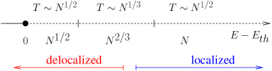
Figure 4: Finite-size scaling of the microcanonical temperature $T$ for the different regimes of $E-E_{th}$, see Eq. (81). $T$ is negative in the whole semiaxis $E-E_{th}>0$, see dashed line. The location of the localization transition is also shown qualitatively.

Let us finally point out that negative temperatures are not a peculiarity of the non-equivalence between canonical and microcanonical ensembles. They exist also in situations where the two ensembles are equivalent, provided the Hamiltonian of the system is a bounded function Cerino et al. (2015); Baldovin et al. (2018); Miceli et al. (2019). On the other hand, in the case of unbounded Hamiltonians, as in the case of the DNLSE, negative temperatures have a physical meaning only within the microcanonical ensemble, thus making ensemble inequivalence a necessary condition for the observation of negative temperature states.

IV.4 Numerical simulations: the pseudo-condensate phase

In this subsection we focus on the equilibrium properties of the pseudo condensate phase as obtained from numerical simulations. Without any loss of generality, we have fixed $a=1$. Accordingly, from Eq. (17) one obtains $\langle\varepsilon\rangle=2$ and $\sigma^{2}=20$, respectively. This, in turn, yields the following values for the spinodal point of the condensate and for the transition point in the scaling variable $\zeta$, as shown in Fig. 3:

$$\zeta_{l} \approx 8.77$$

$$\zeta_{c} \approx 11.05$$ (83)

To well appreciate the pseudo-condensate region, we have focused on a relatively small size, namely $N=128$. With this choice, the threshold energy ${\color[rgb]{0,0,0}e}_{\text{th}}$ for ensemble inequivalence and the localization energy ${\color[rgb]{0,0,0}e}_{c}$ reads off, accordingly, as:

$${\color[rgb]{0,0,0}e}_{\text{th}} = 2a^{2}=2$$

$${\color[rgb]{0,0,0}e}_{c} = {\color[rgb]{0,0,0}e}_{\text{th}}+\frac{\zeta_{c}}{N^{1/3}}\approx 4.2$$ (84)

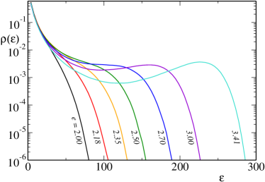
Figure 5: Marginal energy density probability $\rho(\varepsilon)$ (see Eq. (62)) obtained from numerical simulations for $N=128$, $a=1$ and different values of the energy density, namely ${\color[rgb]{0,0,0}e}=2.00,2.18,2.35,2.50,2.70,3.00,3.41$. The threshold energy (per d.o.f.) for the data in figure is ${\color[rgb]{0,0,0}e_{\text{th}}}=2$ while the critical energy is ${\color[rgb]{0,0,0}e_{c}}=4.2$.

Microcanonical equilibrium simulations have been performed by evolving the system with a stochastic algorithm that was introduced in Iubini et al. (2014) and used also in Szavits-Nossan et al. (2014a, b); Iubini et al. (2017a) for the investigation of constraint-driven condensation. This algorithm allows to sample the phase space characterized by fixed values of the quantities:

$$A=\sum_{j=1}^{N}\rho_{j}^{2}\qquad\qquad\qquad E=\sum_{j=1}^{N}\rho_{j}^{4}.$$ (85)

In detail, we have considered local random updates of randomly selected triplets of neighbouring lattice sites $(j-1,j,j+1)$ such that the following constraints are satisfied:

$$\rho_{j-1}^{2}(t+1)+\rho_{j}^{2}(t+1)+\rho_{j+1}^{2}(t+1)~{}~{} = ~{}~{}\rho_{j-1}^{2}(t)+\rho_{j}^{2}(t)+\rho_{j+1}^{2}(t)$$

$$\rho_{j-1}^{4}(t+1)+\rho_{j}^{4}(t+1)+\rho_{j+1}^{4}(t+1)~{}~{} = ~{}~{}\rho_{j-1}^{4}(t)+\rho_{j}^{4}(t)+\rho_{j+1}^{4}(t),$$

where the variable $t$ is the discrete time of the algorithm and is measured in numbers of random moves divided by $N$. To sample the equilibrium microcanonical measure of the model, we have evolved the system for a period of $2^{16}$ time units starting from a partially localized initial condition . By monitoring the evolution of the participation ratio $Y_{2}(E,t)$, we have verified that the relaxation transient was sufficient to ensure relaxation to equilibrium in the range of energies $E$ here considered. After this transient, we have sampled the marginal distribution $\rho(\varepsilon)$ for times up to $t=2^{27}$ units.

Fig. 5 shows $\rho(\varepsilon)$ for increasing values of the total energy density $e<e_{c}$. For sufficiently large values of $e$, a bump is clearly visible in the region of large $\varepsilon$. Therefore, despite the fact that the system is below the localization threshold, we observe that the pseudo-condensate phase is characterized by a process of partial energy localization. In other words, the non-monotonic decay of $\rho(\varepsilon)$ is not enough to conclude that the system is in the localized phase. For this purpose, a finite-size study of $\rho(\varepsilon)$ is necessary.

V Anomalous large-deviation exponent: physical meaning

After the detailed exposition of all our results in the previous sections, it is now worth to rationalize the physical meaning of the anomalous large-deviation exponents we have found, i.e. the exponent $2/3$ for the matching regime and the exponent $1/2$ for the extreme large-deviation regime. Where do these exponents come from? The answer makes reference to some formulae already met in our calculations. For the sake of clarity, let us start with the exponent $1/2$. The behaviour of the entropy (in excess of the backgroud entropy $S_{N}^{\text{back}}(a)$), i.e., $S_{N}-S_{N}^{\text{back}}(a)\sim-N^{1/2}\sqrt{e-e_{th}}$ [see the third line of Eq. (80)], for deviations of order $e-e_{th}\sim 1$, is the true landmark of localization. The exponent $1/2$ comes directly from the interplay between the order of the non-linearity and the conservation constraint on the norm of the wavefunction. In fact, in the microcanonical partition function one has to account both for the conservation constraints on the sum of each variable squared, i.e. $A=\sum_{j=1}^{N}|z_{j}|^{2}$, and on the energy

$$E=\sum_{j=1}^{N}|z_{j}|^{m}$$ (87)

with $m>2$. As a consequence one obtains an expression of the partition function in the form of Eq. (14), where, for $m$ generic, the asymptotic decay of the individual probability is given by

$$f_{\lambda}(\varepsilon_{j})\sim\exp(-\varepsilon^{2/m}_{j}).$$ (88)

As explained in Sec. III.1 and Sec. III.2 it is in force of the asymptotic decay of $f_{\lambda}(\varepsilon_{j})$ in Eq. (88) that the whole partition function in the extreme large-deviation regime behaves (neglecting terms independent of $E$) as:

$$E-E_{th}\sim N ~{}~{}\Longrightarrow~{}~{}\Omega_{N}(A,E)\sim e^{-(E-E_{\text{th}})^{2/m}}$$

$$~{}~{}\Longrightarrow~{}~{}\Omega_{N}(A,E)\sim e^{-N^{2/m}(e-e_{\text{th}})^{2/m}}$$ (89)

so that the total entropy, again neglecting terms which do not depend on $E$, reads

$$E-E_{th}\sim N~{}~{}\Longrightarrow$$

$$S_{N}(A,E)-S_{N}^{\text{back}}(a)\approx-N^{2/m}(e-e_{th})^{2/m}$$

Thus, for the DNLSE case, characterized by the value $m=4$, one has $S_{N}\sim N^{1/2}$. While the generalization of the large-deviation results reported in Majumdar et al. (2005); Szavits-Nossan et al. (2014a); Gradenigo and Majumdar (2019) to the case of generic $m$ is mathematically straightforward, we want to emphasize its physical meaning: a detail of the microscopic interactions of the system, i.e. the order of the non-linearity, is revealed in the presence of localization at the macroscopic scale. It is from the peculiar dependence of the entropy on $N$, or, equivalently, from the dependence of the entropy on the total energy that one can gather information on the microscopic interactions.

The way the exponent $2/3$ comes into play is very similar. It also depends on the order of the non-linearity, though the connection is less straightforward. On the one hand we can say that the value $1/3$ simply comes from the matching between the Gaussian fluctuations and the extreme large deviations of the partition function, as indicated in Eq. (26), which takes place at the scale $E-E_{th}\sim N^{2/3}$, i.e. at $e-e_{th}\sim N^{-1/3}$ . Since the behaviour of extreme large deviations comes directly from the order of the non-linear self-interaction (87), while the shape of Gaussian fluctuations is independent from it, it is easy to argue that the matching scale is solely dictated by the order of the non-linearity. A longer pathway to reach the same conclusion amounts to consider the expansion around $\beta=0$ ($\beta\in\mathbb{C}$) of the “local free-energy” $\log[z(\lambda,\beta)]$ and to single out the scale where the analytic and the non-analytic terms of the expansion are of the same order (see Sec. III.2). As discussed in detail in Sec. III.2, such a scale turns out to be $\beta\sim N^{-1/3}$.

VI Conclusions

In this paper we have shown how to compute the partition function of the Non-Linear Schrödinger Hamiltonian [Eq. (1)] in the microcanonical ensemble and close to the infinite temperature line. This has allowed us to present a clear and coherent scenario for the thermodynamics of this model, also in relation with its dynamical properties. In fact, previous approaches (e.g., see Rasmussen et al. (2000)) provided less transparent interpretations, due to the use of the grand-canonical ensemble for describing also the phase above the line $\beta=0$ (see Fig. 1). By making use of the microcanonical approach, we have been able to show that this is a localized phase, where typically a finite fraction of the whole energy is localized in a few lattice sites. According to Ruelle Ruelle (1969), this is exactly one of the two conditions where equivalence between statistical ensembles does not apply. Indeed, we have shown that the $\beta=0$ line corresponds to the condition where the micro-canonical and grand-canonical ensembles become inequivalent.

We also want to remark that, in a general perspective, the method we have used to compute the microcanonical partition function is valid for lattices in any spatial dimension. There are further results emerging from our study, that merit to be mentioned.

We have shown that for any finite value of the lattice sizes $N$ the microcanonical temperature is negative for $E>E_{\text{th}}$. Moreover, we have found that for finite $N$ the localization transition is placed slightly above the $\beta=0$ line. Consequently, there exists a region (the pseudo-condensate phase) where one can observe negative-temperature states that are not localized. This is a particularly important outcome in the perspective of designing specific experiments of BEC in optical lattices, where such peculiar states could be observed, while avoiding the condensation of a large fraction of atoms onto a single or few sites – a condition that typically destabilizes the condensate. Numerical simulations performed in Iubini et al. (2017b) show that delocalized negative temperature states can be observed also when a sufficiently high thermal gradient is applied by two thermal reservoirs at positive temperatures, coupled to the opposite ends of the DNLSE chain. This tells us that in out-of-equilibrium conditions, the standard thermal phase and the localized one can coexist, thus confirming that the microcanonical approach is consistent with the physics contained in the DNLSE model.

Last, but not least, our analysis highlights how finite-size corrections to thermodynamic observables, like entropy and temperature, are related, in the localized phase, to details of the microscopic interactions.

Beside providing a deeper understanding of the thermodynamics of the DNLSE, the results reported in this paper impact on wider perspectives. We have highlighted the mechanism of localization in the DNLSE from a thermodynamic perspective, clarifying that it is driven exclusively by the interplay between global constraints and non-linear interactions.

This result is significantly different form the typical phenomenon of Many-Body Localization (MBL) Altman (2018), which is often framed in the context of weakly perturbed integrable models whose quantum unperturbed dynamics is characterized by the existence of as many integrals of motion as degrees of freedom Ros et al. (2015).

We point out that localization of the DNLSE is not due to disorder or to the proximity in parameter space to a linear model. The high energy limit is in a sense an “effectively integrable limit”, but the (independent) individual degrees of freedom are non-linear oscillators.

This basic consideration at least challenges the generality of the MBL approach, since localization in interacting-particle models can be observed in the present case without the need of imposing perturbatively small non-linearities. Nonetheless, analogies with the MBL approach are still traceable. First of all, the DNLSE is a genuine many-body model, because it represents a semiclassical limit of the Bose-Hubbard Hamiltonian Franzosi et al. (2011). Second, in the high-energy localized phase the DNLSE hamiltonian dynamics typically drives the systems to a multi-breather state Franzosi et al. (2011); Iubini et al. (2019, 2013). Each breather can be interpreted as the dynamical solution of an integrable nonlinear oscillator of sufficiently high energy. Even in the presence of a background component, breathers can survive over extremely long time lapses, due to their very weak interaction with the lattice background and, accordingly, with any other breather. On the other hand, the number of breathers is not extensive and slowly fluctuates in time Iubini et al. (2013).

VII Appendices

VII.1 Derivation of the rate function $\chi(\zeta)$ in the intermediate matching regime

In this Appendix we illustrate how to obtain an estimate of the integral in Eq. (43), making use of the saddle point approximation, valid in the limit of large values of $N$. We are dealing with the following expression

$${\color[rgb]{0,0,0}\mathcal{C}(\lambda,\zeta)}=N\int_{\Gamma_{(+)}}\frac{d\beta}{i}\frac{1}{\sqrt{2\pi\langle\varepsilon\rangle N^{1/3}\beta}}~{}e^{N^{1/3}F_{\zeta}(\lambda,\beta)}$$ (91)

where the non-negative quantity $\zeta$ is defined in Eq.(29), and $\lambda$ can be assumed, for the sake of simplicity at this stage of the calculations, to be a positive free parameter. In practice, we have to find under which conditions the function

$$F_{\zeta}(\lambda,\beta)=\beta\zeta+\frac{10}{\lambda^{4}}\,\beta^{2}+\frac{\lambda^{2}}{4\beta}\,.$$ (92)

has a maximum for negative values of $\beta$, since the contour $\Gamma_{(+)}$, along which this integral has to be evaluated, lies in the upper left quadrant of the complex $\beta$-plane. At variance with Eq.(44), in the above expression of $F_{\zeta}(\lambda,\beta)$ we have made explicit its dependence on $\lambda$, making use of Eqs. (17). For the sake of simplicity, let us introduce the shorthand notations $F_{\zeta}^{\prime}(\lambda,\beta)$ and $F_{\zeta}^{\prime\prime}(\lambda,\beta)$ for the first and second derivatives of $F_{\zeta}(\lambda,\beta)$ with respect to $\beta$. The saddle point equation to be solved is

$$F_{\zeta}^{\prime}(\lambda,\beta)=\zeta+\frac{20}{\lambda^{4}}\,\beta-\frac{\lambda^{2}}{4\beta^{2}}=0$$ (93)

It turns out that the position of the three roots of this equation in the complex $\beta$-plane depend on the value of $\zeta$. More precisely, there exists a specific value of this non-negative parameter

$$\zeta_{l}=3\cdot\frac{5^{2/3}}{\lambda^{2}}$$ (94)

such that for $\zeta<\zeta_{l}$ there are two complex conjugate roots with negative real part and one real root on the positive axis, i.e. the saddle point equation does not provide us with any acceptable solution. Conversely, for $\zeta>\zeta_{l}$ there are three real roots $\beta_{1}<\beta_{2}<\beta_{3}$: the first two roots are negative, while the third one is positive (therefore, uninteresting for our calculation).

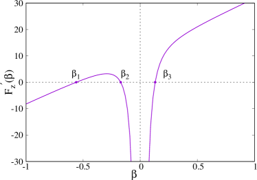
Figure 6: Plot of $F_{\zeta}^{\prime}(\lambda,\beta)$ as a function of $\beta\in\mathbb{R}$ for $\lambda=1$ and $\zeta=12$.

In order to make clear the latter scenario, in Fig. 6 we plot $F_{\zeta}^{\prime}(\lambda,\beta)$ as a function of $\beta\in\mathbb{R}$ for $\lambda=1$ and $\zeta=12>\zeta_{l}$. Making reference to this picture we can explain the origin of $\zeta_{l}$: it identifies the bifurcation point where, by decreasing $\zeta$, the two negative real roots $\beta_{1}$ and $\beta_{2}$ eventually coincide and then they become complex conjugate. In practice, the value of $\zeta_{l}$ can be obtained by imposing the condition that the value of $F_{\zeta}^{\prime}(\lambda,\beta)$ at its maximum, located in the negative value $\beta_{m}\in(\beta_{1},\beta_{2})$ vanishes. The value of $\beta_{m}=-\frac{\lambda^{2}}{2\cdot 5^{1/3}}$ is obtained by imposing the condition $F_{\zeta}^{\prime\prime}(\lambda,\beta_{m})=0$, while $\zeta_{l}$ is finally determined by the condition $F_{\zeta}^{\prime}(\lambda,\beta_{m})=0$. Another important outcome that we can obtain by direct visual inspection of Fig.6 is that $F_{z}^{\prime\prime}(\lambda,\beta_{1})>0$ and $F_{z}^{\prime\prime}(\lambda,\beta_{2})<0$, from which we can conclude that the maximum of $F_{\zeta}(\lambda,\beta)$ is at $\beta_{2}$, which is the saddle-point solution that we are looking for.

Summarizing, we finally obtain the saddle-point estimate

$${\color[rgb]{0,0,0}\mathcal{C}(\lambda,\zeta)}\approx\exp[-N^{1/3}\chi(\zeta)]\$$ (95)

where the rate function $\chi(\zeta)$ is given by

$$\chi(\zeta)=-F_{\zeta}(\lambda,\beta=\beta_{2})=-\beta_{2}\,\zeta-\frac{10}{\lambda^{4}}\beta_{2}^{2}-\frac{\lambda^{2}}{4\beta_{2}}$$ (96)

Making use of the saddle point equation (93), one can further simplify the above equation as follows:

$$\chi(\zeta)=-\frac{\zeta\beta_{2}}{2}-\frac{3\lambda^{2}}{8\beta_{2}}\,.$$ (97)

VII.2 Properties of $\chi(\zeta)$

Here we describe the rate function $\chi(\zeta)$ in the range $\zeta_{l}<\zeta<\infty$, where $\zeta_{l}$ is given in Eq. (94). As discussed in the previous Appendix, for $\zeta=\zeta_{l}$ the roots $\beta_{1}$ and $\beta_{2}$ coincide with $\beta_{m}=-\frac{\lambda^{2}}{2\cdot 5^{1/3}}$. Substituting this value into Eq. (97), one obtains

$$\chi(\zeta_{l})=\frac{3}{2}\,\left(\frac{10}{\lambda^{2}}\right)^{2/3}\,,$$ (98)

as reported in the first line of Eq. (47).

Finding the behavior of $\chi(\zeta)$ for large values of $\zeta$ can be easily obtained making use of a suitable reparametrization of the root $\beta_{2}$ in the form

$$\beta_{2}=-\frac{\lambda}{2\sqrt{\zeta}}\theta_{\zeta}\,.$$ (99)

Then Eq. (93) can be rewritten in the form

$$-b(\zeta)~{}\theta_{\zeta}^{3}+\theta_{\zeta}^{2}-1=0,$$ (100)

where

$$b(\zeta)=\frac{10}{\lambda^{3}}\frac{1}{\zeta^{3/2}}.$$ (101)

Note that, due to the change of sign in passing from $\beta_{2}$ to $\theta_{\zeta}$, we have to find the smallest positive root $\theta_{\zeta}$ in Eq. (100). Also Eq. (97) can be rewritten in terms of $\theta_{\zeta}$ as follows

$$\chi(\zeta)=\sqrt{\zeta}~{}\frac{\lambda}{4}~{}\frac{\theta_{\zeta}^{2}+3}{\theta_{\zeta}}\,.$$ (102)

From Eqs. (100) and (101) it follows immediately that $\theta_{\zeta}\to 1$ for $\zeta\to\infty$. Hence, for large $\zeta$ (or equivalently small $b(\zeta)$), we obtain a perturbative solution of Eq. (100), which at leading order reads

$$\theta_{\zeta}=1+\frac{b(\zeta)}{2}+\mathcal{O}\left({b(\zeta)}^{2}\right)\,.$$ (103)

By substituting this perturbative solution into Eq. (102) we finally obtain the behavior of $\chi(\zeta)$ for large values of $\zeta$ in the form

$$\chi(\zeta)=\lambda~{}\sqrt{\zeta}-\frac{5}{2\lambda^{2}}\frac{1}{\zeta}+\mathcal{O}\left(\frac{1}{\zeta^{5/2}}\right)\,,$$ (104)

as reported in the second line of Eq. (47).

More generally, the explicit expression of the smallest positive root of Eq. (100) can be obtained making use of Mathematica; it reads:

$$\theta_{\zeta}=\frac{1}{3b_{\zeta}}+\frac{1}{3\cdot 2^{2/3}b_{\zeta}}\frac{(1-i\sqrt{3})}{\left(-2+27b_{\zeta}^{2}+3\sqrt{-12+81b_{\zeta}^{2}}\right)^{1/3}}+\frac{1}{3\cdot 2^{4/3}b_{\zeta}}(1+i\sqrt{3})\left(-2+27b_{\zeta}^{2}+3\sqrt{-12+81b_{\zeta}^{2}}\right)^{1/3}$$ (105)

where we have introduced the shorthand notation $b_{\zeta}$ for $b(\zeta)$. By making use of Eq. (94), we can conveniently rewrite $b_{\zeta}$ in the dimensionless form

$$b_{\zeta}^{2}=\frac{1}{2}~{}\left(\frac{2}{3\,r}\right)^{3}\,,$$ (106)

where $r=\zeta/\zeta_{l}\geq 1$. Accordingly, we can also rewrite the saddle-point solution  (105) in the form

$$\theta_{\zeta}\equiv\theta(r)=\frac{\sqrt{3}}{4}r^{3/2}\left[2+\frac{(1-i\sqrt{3})}{g(r)}+(1+i\sqrt{3})g(r)\right]$$ (107)

where

$$g(r)=\frac{1}{r}\left(1+i~{}\sqrt{r^{3}-1}\right)^{2/3}.$$ (108)

By multiplying both the numerator and the denominator of $\theta(r)$ by $(1-i~{}\sqrt{r^{3}-1})^{2/3}$ one obtains the following expression for the saddle-point solution:

$$\theta(r)=\frac{\sqrt{3}}{4}r^{3/2}\left[2+\frac{1}{r}\left(\xi~{}u_{r}^{2/3}+\overline{\xi}~{}\overline{u}_{r}^{2/3}\right)\right],$$ (109)

where $\xi$ and $u_{r}$ denote, respectively, a complex number and a complex function of the real variable $r$:

$$\xi = 1+i\sqrt{3}$$

$$u_{r} = 1+i~{}\sqrt{r^{3}-1}.$$ (110)

The overbars in Eq.(109) denote the complex conjugate quantities. After some straightforward algebra, one obtains the following expression of the saddle-point solution

$$\theta(r)=\frac{\sqrt{3}}{2}r^{3/2}\left[1+2\cos\left(\frac{\pi}{3}+\frac{2}{3}\textrm{arctan}(\sqrt{r^{3}-1})\right)\right]$$ (111)

Summarizing all these calculations, we finally observe that from Eq.(102) it follows that the rate function $\chi(\zeta)$ can be written explicitly in terms of this explicit saddle-point solution.

VII.3 The critical value $\zeta_{c}$

In this appendix we obtain the critical value $\zeta_{c}$, which is identified by the matching condition $\chi(\zeta_{c})=\zeta_{c}^{2}/(2\sigma^{2})$, i.e., the value at which the two branches in Fig. 3 cross each other. Making use of the definitions introduced in the previous Appendix we can write explicitly the matching condition in the form

$$\sqrt{\zeta_{c}}\frac{\lambda}{4}\,\left[\frac{\theta(r_{c})^{2}+3}{\theta(r_{c})}\right]=\frac{\lambda^{4}}{40}\zeta_{c}^{2}\,,$$ (112)

where $r_{c}=\zeta_{c}/\zeta_{l}$. Taking into account Eq.(94), the previous equation can be rewritten as follows:

$$\frac{\theta^{2}(r_{c})+3}{\theta(r_{c})}=\frac{3^{3/2}}{2}\,r_{c}^{3/2}\,.$$ (113)

A shortcut to obtain the expected result amounts to substitute this relation directly into the equation

$$-\frac{1}{\sqrt{2}}\,\left(\frac{2}{3}\right)^{3/2}\,r^{-3/2}\,\theta(r)^{3}+\theta(r)^{2}-1=0\,,$$ (114)

which is a suitable way of rewriting the saddle-point equation (100) in terms of the adimensional variable $r$. Thus one obtains the simple result

$$\theta(r_{c})=\sqrt{\frac{3}{2}}\,.$$ (115)

As a final step it remains to substitute this result into Eq.(113) and we finally obtain

$$r_{c}=\frac{\zeta_{c}}{\zeta_{l}}=2^{1/3}$$ (116)

One can obtain an immediate check of this result by computing from Eq. (111) $\theta(r_{c})=\sqrt{\frac{3}{2}}$, as expected.

References

- Trombettoni and Smerzi (2001) A. Trombettoni and A. Smerzi, Physical Review Letters 86, 2353 (2001).
- Franzosi et al. (2011) R. Franzosi, R. Livi, G.-L. Oppo, and A. Politi, Nonlinearity 24, R89 (2011).
- Eisenberg et al. (1998) H. Eisenberg, Y. Silberberg, R. Morandotti, A. Boyd, and J. Aitchison, Physical Review Letters 81, 3383 (1998).
- Johansson and Rasmussen (2004) M. Johansson and K. Ø. Rasmussen, Physical Review E 70, 066610 (2004).
- Livi et al. (2006) R. Livi, R. Franzosi, and G.-L. Oppo, Physical Review Letters 97, 060401 (2006).
- Rasmussen et al. (2000) K. Rasmussen, T. Cretegny, P. G. Kevrekidis, and N. Grønbech-Jensen, Physical Review Letters 84, 3740 (2000).
- Iubini et al. (2019) S. Iubini, L. Chirondojan, G.-L. Oppo, A. Politi, and P. Politi, Physical Review Letters 122, 084102 (2019).
- Franzosi (2011) R. Franzosi, Journal of Statistical Physics 143, 824 (2011).
- Iubini et al. (2013) S. Iubini, R. Franzosi, R. Livi, G.-L. Oppo, and A. Politi, New Journal of Physics 15, 023032 (2013).
- Rumpf and Newell (2001) B. Rumpf and A. C. Newell, Physical Review Letters 87, 054102 (2001).
- Rumpf (2004) B. Rumpf, Physical Review E 69, 016618 (2004).
- Rumpf (2007) B. Rumpf, EPL (Europhysics Letters) 78, 26001 (2007).
- Rumpf (2008) B. Rumpf, Physical Review E 77, 036606 (2008).
- Rumpf (2009) B. Rumpf, Physica D: Nonlinear Phenomena 238, 2067 (2009).
- Iubini et al. (2014) S. Iubini, A. Politi, and P. Politi, Journal of Statistical Physics 154, 1057 (2014).
- Iubini et al. (2017a) S. Iubini, A. Politi, and P. Politi, Journal of Statistical Mechanics: Theory and Experiment 2017, 073201 (2017a).
- Barré and Mangeolle (2018) J. Barré and L. Mangeolle, Journal of Statistical Mechanics: Theory and Experiment 2018, 043211 (2018).
- Cherny et al. (2019) A. Y. Cherny, T. Engl, and S. Flach, Physical Review A 99, 023603 (2019).
- Corberi (2015) F. Corberi, Journal of Physics A: Mathematical and Theoretical 48, 465003 (2015).
- Corberi (2017) F. Corberi, Physical Review E 95, 032136 (2017).
- Corberi et al. (2019) F. Corberi, O. Mazzarisi, and A. Gambassi, Journal of Statistical Mechanics: Theory and Experiment 2019, 104001 (2019).
- Szavits-Nossan et al. (2014a) J. Szavits-Nossan, M. R. Evans, and S. N. Majumdar, Physical Review Letters 112, 020602 (2014a).
- Szavits-Nossan et al. (2014b) J. Szavits-Nossan, M. R. Evans, and S. N. Majumdar, Journal of Physics A: Mathematical and Theoretical 47, 455004 (2014b).
- Szavits-Nossan et al. (2016) J. Szavits-Nossan, M. R. Evans, and S. N. Majumdar, Journal of Physics A: Mathematical and Theoretical 50, 024005 (2016).
- Majumdar et al. (2005) S. N. Majumdar, M. R. Evans, and R. K. P. Zia, Physical Review Letters 94, 180601 (2005).
- Evans et al. (2006) M. R. Evans, S. N. Majumdar, and R. K. P. Zia, Journal of Statistical Physics 123, 357 (2006).
- Evans and Hanney (2005) M. R. Evans and T. Hanney, Journal of Physics A: Mathematical and General 38, R195 (2005).
- Majumdar (2010) S. N. Majumdar, Exact Methods in Low-dimensional Statistical Physics and Quantum Computing: Lecture Notes of the Les Houches Summer School: Volume 89, July 2008 , 407 (2010).
- Gradenigo and Majumdar (2019) G. Gradenigo and S. N. Majumdar, Journal of Statistical Mechanics: Theory and Experiment 2019, 053206 (2019).
- Note (1) The normalization of can be verified from a calculation analogous to the one in Eq. (61) for the microcanonical average of the constant function .
- Gradenigo and Bertin (2017) G. Gradenigo and E. Bertin, Entropy 19, 517 (2017).
- Gradenigo et al. (2020) G. Gradenigo, S. Iubini, R. Livi, and S. N. Majumdar, (2020).
- Cerino et al. (2015) L. Cerino, A. Puglisi, and A. Vulpiani, Journal of Statistical Mechanics: Theory and Experiment 2015, P12002 (2015).
- Baldovin et al. (2018) M. Baldovin, A. Puglisi, and A. Vulpiani, Journal of Statistical Mechanics: Theory and Experiment 2018, 043207 (2018).
- Miceli et al. (2019) F. Miceli, M. Baldovin, and A. Vulpiani, Physical Review E 99, 042152 (2019).
- Note (2) For a fixed value of the total energy and system size , we have chosen a set of initial conditions where a fraction of sites has a value of local mass while in the remaining part of the system the local mass is , with . The parameters and are solutions of the equations and .
- Ruelle (1969) D. Ruelle, Statistical mechanics: Rigorous results, W.A. Benjamin Inc. (1969).
- Iubini et al. (2017b) S. Iubini, S. Lepri, R. Livi, G.-L. Oppo, and A. Politi, Entropy 19, 445 (2017b).
- Altman (2018) E. Altman, Nature Physics 14, 979 (2018).
- Ros et al. (2015) V. Ros, M. Müller, and A. Scardicchio, Nuclear Physics B 891, 420 (2015).