CHANDRA OBSERVATIONS OF THE SPECTACULAR A3411–12 MERGER EVENT

Abstract

We present deep Chandra observations of A3411–12, a remarkable merging cluster that hosts the most compelling evidence for electron re-acceleration at cluster shocks to date. Using the $Y_{X}-M$ scaling relation, we find $r_{500}\sim 1.3$ Mpc, $M_{500}=(7.1\pm 0.7)\times 10^{14}\ M_{\rm{\odot}}$, $kT=6.5\pm 0.1$ keV, and a gas mass of $M_{\rm g,500}=(9.7\pm 0.1)\times 10^{13}M_{\odot}$. The gas mass fraction within $r_{500}$ is $f_{\rm g}=0.14\pm 0.01$. We compute the shock strength using density jumps to conclude that the Mach number of the merging subcluster is small ($M\leq 1.15_{-0.09}^{+0.14}$). We also present pseudo-density, projected temperature, pseudo-pressure, and pseudo-entropy maps. Based on the pseudo-entropy map we conclude that the cluster is undergoing a mild merger, consistent with the small Mach number. On the other hand, radio relics extend over Mpc scale in the A3411–12 system, which strongly suggests that a population of energetic electrons already existed over extended regions of the cluster.

1 Introduction

Galaxy cluster mergers are the most energetic events in the present day Universe and involve kinetic energies on the order of $\sim 10^{63-64}$ erg. Direct evidence for cluster mergers has been found from the morphology of the X-ray emission (e.g., Jones & Forman, 1984, 1999; Mohr et al., 1995; Buote & Tsai, 1996; Jeltema et al., 2005; Laganá et al., 2010; Andrade-Santos et al., 2012, 2013) and the presence of shocks (e.g., Markevitch et al., 2002) in the intracluster medium (ICM), as well as from the asymmetric spatial and velocity distributions of cluster galaxy populations (Dressler & Shectman, 1988).

The identification and study of merging clusters is of considerable astrophysical interest for several reasons. First, such major mergers are rare events, and have a profound, long lasting influence on the thermodynamic evolution of the ICM. Major mergers are believed to be responsible for the general division of clusters into cool-core and non-cool-core clusters (Henning et al., 2009). Mergers can also affect a wide range of other cluster related phenomena, including AGN activity in cluster galaxies (Ma et al., 2010; Sobral et al., 2015) and star formation (Laganá et al., 2008; Sobral et al., 2015; Stroe et al., 2015, 2017). Second, cluster mergers are an ideal laboratory to study the properties of dark matter. X-ray and optical (lensing) studies have put strong constraints on the self-interaction of dark matter and have shown that it must be nearly collisionless (Clowe et al., 2004, 2006; Bradač et al., 2006, 2008; Randall et al., 2008; Dawson et al., 2012).

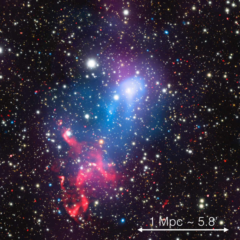
Figure 1: Composite image of the A3411–A3412 field: optical (Subaru – RGB), 0.5-2.0 keV X-ray (Chandra – in blue), 325 and 610 MHz radio (GMRT – in red), and the galaxy density distribution (purple). A3411–12 presents a clear cool core in the north and a large (Mpc scale) radio relic in the south. In the north there is an overdensity of galaxies at the cluster redshift, located in the cool core (X-ray: bright blue, galaxy density: purple) region, whereas another peak in the galaxy distribution (purple) is seen in the relic region (red) in the south.

Simulations of large-scale structure formation show that galaxy clusters grow through gas accretion from large-scale filaments and mergers of smaller clusters and groups. These mergers are characterized by the enormous amounts of energy involved ($\sim 10^{64}$ erg), long lifetimes (Gyr), and large physical scales (Mpc). Most of the gravitational energy released during a merger event is converted to thermal energy via shocks and turbulence (see Markevitch & Vikhlinin, 2007, for a review). In addition, a small fraction ($<1$%) of the shock energy could be channeled into the acceleration of cosmic rays (CR). In the presence of magnetic fields these CR then emit synchrotron radiation, which can be observed with radio telescopes.

The elongated and arc-like radio sources that trace cluster merger shocks are commonly called radio relics (Feretti et al., 2012, see Figure 1). A major problem in our understanding is how these low-Mach number ($\mathcal{M}$) cluster merger shocks can accelerate enough particles to explain the observed radio synchrotron brightness. According to standard diffusive shock acceleration theory (DSA; Drury, 1983), the acceleration efficiency is very low for $\mathcal{M}\lesssim 4$ shocks, and the existence of radio relics is therefore very puzzling (e.g., Hong et al., 2014; Kang et al., 2012).

Two main particle acceleration mechanisms have been proposed to explain radio relics:

(1) Shock acceleration: Particles gain energy via multiple crossing of the shock front, however, it is very hard to reconcile the low acceleration efficiency with the bright radio relics.

(2) Re-acceleration: Shocks re-accelerate a population of pre-existing (“fossil”) relativistic electrons via DSA (Markevitch et al., 2005), avoiding the low acceleration efficiency problem. Good source candidates for these fossil electrons are radio galaxies (common in clusters).

1.1 A3411–12

A3411–12 (also known as PLCKESZ G241.97+14.85 – see Figure 1) is a relatively nearby ($z=0.1687$) merging cluster presenting a large ($\sim 0.7$ Mpc) radio relic (van Weeren et al., 2013; Giovannini et al., 2013). van Weeren et al. (2013) showed that A3411–12 is a merging system, with the projected merger axis oriented SE-NW (see Figure 1) with A3411 in the NW and A3412 in the SE. Chandra X-ray image shows that the cluster has a cometary shape with a well-defined subcluster core visible in the northwestern part of the system (A3411). Fainter X-ray emission is found surrounding the subcluster core and this emission seems to be part of a second, larger subcluster (A3412). There is no clear surface brightness peak corresponding to the primary cluster core (A3412 – see Figure 2), which suggests the primary cluster has been disrupted by the collision with the subcluster (A3411 – see Figure 2), as has been the case for A2146 (Russell et al., 2011; Menanteau et al., 2012). Giovannini et al. (2013) have also found that the radio halo at the center of A3411-12 has a low power (${\rm log}~{}P=23.16{\rm~{}W~{}Hz}^{-1}$). The global ICM temperature of A3411–12 is $\sim$ 6 keV and its X-ray 0.5–2.0 keV luminosity is $2.8\times 10^{44}\rm~{}erg~{}s^{-1}$ within $r_{500}$ = 1.34 Mpc (van Weeren et al., 2013).

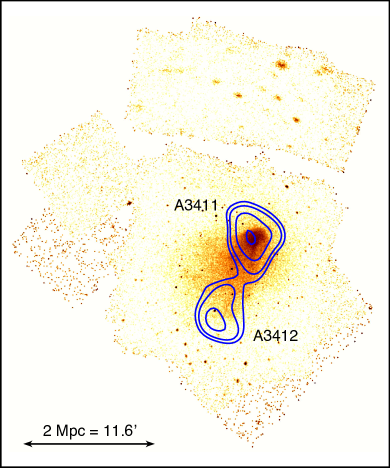
Figure 2: 0.5–2.0 keV, background subtracted, flat-field Chandra image of the A3411–12 field overlaid by galaxy iso-density contours in blue.

More recently, van Weeren et al. (2017) found, in the merging galaxy cluster A3411–12, the most compelling evidence for re-acceleration at cluster shocks to date. The authors identified a tailed radio galaxy connected to the relic. In addition, spectral flattening is observed at the location where the fossil plasma meets the relic and, at the same location, an X-ray surface brightness edge is observed.

van Weeren et al. (2017) also presented a clustering analysis applied to the three-dimensional galaxy distribution (right ascension, declination, and redshift) of their spectroscopic sample of cluster members (obtained with Keck). They considered mixtures of 1 to 7 multivariate Gaussian components. They found that, of the models considered, the two-component Gaussian model is the most favored one, indicating a bi-modal distribution. They also investigated the redshift and velocity dispersion of each subcluster. They found similar velocity dispersions for the northern (A3411) and southern (A3412) subclusters, $1110^{+100}_{-80}\rm~{}km~{}s^{-1}$ and $1190^{+100}_{-90}\rm~{}km~{}s^{-1}$, respectively. These velocity dispersions translated into mass estimates of $1.4^{+0.4}_{-0.3}\times 10^{15}M_{\odot}$ and $1.8^{+0.5}_{-0.4}\times 10^{15}M_{\odot}$ for the A3411 and A3412 subclusters, respectively. With the mass estimates and redshift distributions, they concluded that core passage for the A3411-A3412 merger event occurred about $\sim$ 1 Gyr before the photons Chandra collected were emitted and that the plane of the merger event is seen relatively close ($9^{\circ}$–$41^{\circ}$) to the plane of the sky crossing the cluster center, implying that the shock is seen close to edge-on. It is worthy mentioning that in the current work we find a much smaller total mass for the system of $M_{\rm 500}=(7.14\pm 0.65)\times 10^{14}M_{\odot}$, in very good agreement with the Planck estimated mass of $M_{\rm 500}=(6.59\pm 0.31)\times 10^{14}M_{\odot}$ (Planck Collaboration et al., 2016).

In this paper we characterize this cluster based on Chandra X-ray observations, present temperature, density, pressure, and entropy maps, as well as density jumps related to cold and shock fronts. We show that if indeed the density jumps trace shocks, they are mild, indicating that a population of energetic electrons already existed over extended regions of the cluster based on the extension of the radio relics in the A3411–12 system. The cosmology assumed for our analysis has $\Omega_{\rm M}=0.3$, $\Omega_{\Lambda}=0.7$ and $H_{0}=70$ km s^-1Mpc^-1, implying a linear scale of $2.88\rm~{}kpc~{}arcsec^{-1}$ at the A3411–12 luminosity distance of 812 Mpc ($z=0.1687$). All uncertainties are 68% confidence level, unless otherwise stated.

2 X-ray observations and data reduction

We observed A3411 with the Chandra  X-ray Observatory (ACIS-I detectors, VF mode, ObsIds 13378, 15316 – PI Murray, and 17193, 17496, 17583, 17585, 17584 – PI van Weeren). The data were reduced using the software CHAV which follows the processing described in Vikhlinin et al. (2005), applying the calibration files CALDB 4.6.7. The data processing includes corrections for the time dependence of the charge transfer inefficiency and gain, and a check for periods of high background (none were found – the total exposure time is 211 ks). Also, readout artifacts were subtracted and standard blank sky background files were used for background subtraction. Figure 2 shows the combined image of all observations in the 0.5–2.0 keV energy band.

Since the focus of this paper is solely on X-ray data and their results, we refer the reader to van Weeren et al. (2017) for the details on the optical and radio reductions performed to create the image displayed on Figure 1.

3 Overall characteristics of the cluster

3.1 Emission measure profile

In this section we outline the procedures used to compute the emission measure profile. We refer the reader to Vikhlinin et al. (2006) for a detailed description of the method.

First we detected compact sources using wavdect in the 0.7–2.0 keV or 2.0–7.0 keV bands and then masked these from the spectral and spatial analyses (we also masked the bullet (cool-core in A3411) – see top left panel of Figure 3). We then measured the surface brightness profiles in the 0.7–2.0 keV energy band, which maximizes the signal to noise ratio in Chandra data. The readout artifacts and blank-field background (see section 2.3.3 of Vikhlinin et al., 2006) were subtracted from the X-ray images, and the result was exposure-corrected using exposure maps (computed assuming an absorbed optically-thin thermal plasma with $kT=5.0$ keV, abundance = 0.3 $Z_{\sun}$, plus the Galactic column density that include corrections for bad pixels and CCD gaps, but do not take into account spatial variations of the effective area. Finally, we subtracted any small uniform component corresponding to soft X-ray foreground adjustments that may be required.

Table 1: Parameters for the emission measure profile (Equation 1)

$n_{0}$	$r_{\rm c}$	$r_{\rm s}$	$\alpha$	$\beta$	$\gamma$	$\epsilon$	$n_{02}$	$r_{\rm c2}$	$\beta_{2}$
($\rm 10^{-3}~{}cm^{-3}$)	(kpc)	(kpc)					($\rm 10^{-3}~{}cm^{-3}$)	(kpc)
$1.12\pm 0.19$	$260\pm 3$	$262\pm 9$	$0.00\pm 0.10$	$0.75\pm 0.20$	$0.79\pm 0.11$	$0.04\pm 0.10$	$1.23\pm 0.07$	$736\pm 52$	$0.96\pm 0.06$

Note. — Columns list best fit values for the parameters given by Equation 1.

Table 2: Parameters for the Temperature Profile (Equations 2 and 3)

$T_{0}$	$T_{\rm min}$	$r_{\rm t}$	$r_{\rm cool}$	$a_{\rm cool}^{\dagger}$	$a^{\dagger}$	$b$	$c$
(keV)	(keV)	(kpc)	(kpc)
$13.0\pm 1.7$	$5.2\pm 0.7$	$545\pm 173$	$400\pm 104$	1.9	0	$5.0\pm 1.3$	$3.1\pm 1.9$

Note. — Columns list best fit values for the parameters given by Equations 2 and 3. ^† fixed value.

Following these steps, we extracted the surface brightness profiles in narrow concentric annuli ($r_{\rm out}/r_{\rm in}=1.05$) centered on the X-ray centroid (determined excluding the masked regions) and computed the Chandra area-averaged effective area for each annulus (see Vikhlinin et al., 2005, for details on calculating the effective area). Using the observed projected temperature, effective area, and metallicity as a function of radius, we converted the Chandra count rate in the 0.7–2.0 keV band into the emission integral, ${\rm EI}=\int n_{\rm e}n_{\rm p}dV$, within each cylindrical shell. The X-ray morphology of A3411–12 exhibits an irregular shape (see Figure 2), however, this is mostly due to the bullet in the northern part of the cluster. When we mask the bullet, the cluster exhibits a more elongated and symmetrical shape. To compute the emission measure and temperature profiles we assumed spherical symmetry. In this case, the spherical assumption is expected to have only small effects on the total mass of the cluster when using $Y_{\rm X}$ as a proxy, as presented by Kravtsov et al. (2006). They showed that $Y_{\rm X}$ is a robust mass indicator with remarkably low scatter of only $\approx 5\%$–$7\%$ in $M_{500}$ for fixed $Y_{\rm X}$, regardless of whether the cluster is relaxed or not. We then fit the emission measure profile assuming the gas density profile follows Vikhlinin et al. (2006):

$$n_{\rm e}n_{\rm p} = n_{0}^{2}\frac{(r/r_{\rm c})^{-\alpha}}{(1+r^{2}/r_{\rm c}^{2})^{3\beta-\alpha/2}}\frac{1}{(1+r^{\gamma}/r_{\rm s}^{\gamma})^{\epsilon/\gamma}}+$$ (1)

$$\frac{n^{2}_{02}}{(1+r^{2}/r_{\rm c2}^{2})^{3\beta_{2}}}.$$

This relation is based on a classic $\beta$-model, modified to account for the power-law type cusp and the steeper emission measure slope at large radii. In addition, a second $\beta$-model is included, giving extra freedom to characterize the cluster core. For further details on this equation we refer to Vikhlinin et al. (2006). The relation between the electron number density and gas mass density is given by $\rho_{\rm g}=\mu_{\rm e}n_{\rm e}m_{\rm a}$, where $m_{\rm a}$ is the atomic mass unit and $\mu_{\rm e}$ is the mean molecular weight per electron. For a typical metallicity of 0.3 $Z_{\odot}$, the reference values from Anders & Grevesse (1989) yield $\mu_{\rm e}=1.17058$ and $n_{\rm e}/n_{\rm p}=1.1995$, where $n_{\rm p}$ is the proton number density. The best fit parameters of Equation 1 are listed in Table 1. Figure 3 presents the best fit emission measure profile, as well as the density and gas mass profiles derived from the best fit emission measure. The gas mass profile is then used to compute the total mass using the $Y_{\rm x}$ relation (Section 4).

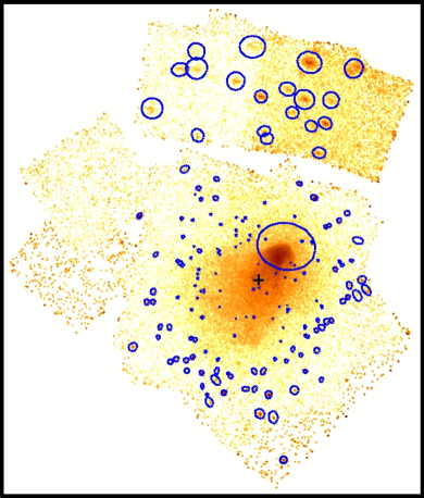
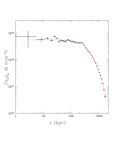
Figure 3: X-ray image (upper left), projected emissivity (upper right), gas density (lower left), and enclosed gas mass (lower right) profiles for A3411–12. Top left panel shows the 0.5-2.0 keV, background-subtracted, exposure map corrected ACIS-I image. The total filtered Chandra exposure is 211 ks. Blue ellipses correspond to the masked X-ray point sources (we also masked the bullet (cool-core in A3411)) and the black cross corresponds to the cluster center (determined by computing the X-ray centroid in a circle of $\sim$ 1.3 Mpc radius including the cool-core). Top right panel shows the projected emissivity profile. The solid line shows the emission measure integral of the best fit to the emissivity profile given by Equation (1) assuming $n_{\rm e}=1.1995\times n_{\rm p}$, where $n_{\rm e}$ and $n_{\rm p}$ are the electron and proton number densities, respectively. Bottom left panel shows the electron number density profile. The solid line shows the electron number density profile obtained from the emissivity profile given by Equation (1). Bottom right panel shows the gas mass profile, with the dashed vertical line indicating $r_{500}$. The dashed lines in the electron number density and gas mass profiles show the 68% confidence range.

3.2 Gas Temperature Radial Profiles

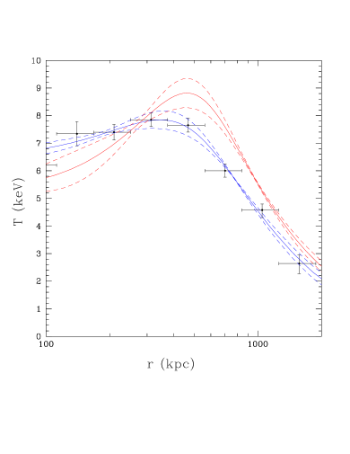
Figure 4: Azimuthally averaged, radial temperature profile. Observed projected temperatures are shown by points with error bars. The 3D model and its projected effective temperatures (the latter to be compared with the data) are shown by the red and blue curves, respectively. Dashed lines show the 1$\sigma$ uncertainty ranges.

Most clusters present a temperature profile that has a broad peak within 0.1–0.2 $r_{200}$. Vikhlinin et al. (2006) present a 3D temperature profile that describes these general features. At large radii, the temperature profile can be reasonably well represented as a broken power law with a transition region:

$$T(r)=\frac{(r/r_{t})^{-a}}{(1+(r/r_{t})^{b})^{c/b}}.$$ (2)

At small radii, the temperature profile can be described as

$$T_{\text{cool}}(r)=(x+T_{\text{min}}/T_{0})/(x+1),$$ (3)

where $x=(r/r_{\text{cool}})^{a_{\text{cool}}}$. The final analytical expression for the 3D temperature profile is,

$$T_{\mathrm{3D}}(r)=T_{0}\times T_{\text{cool}}(r)\times T(r).$$ (4)

This temperature model has significant functional freedom (8 parameters) and can adequately describe almost any smooth temperature distribution. Thus, we use this model, from Vikhlinin et al. (2006), to describe the temperature distribution of the hot gas in A3411–12.

To construct the temperature profile, we extracted spectra from 7 annuli in the radial range from $\sim 100$ to $\sim 2000$ kpc (logarithmically spaced in distance) and fit them with an absorbed APEC model. For the fitting we fixed NH to the Galactic value of $5.92\times 10^{20}$ (see Section 3.1). We then followed the procedures described above to obtain the 2D and 3D temperature profiles. The measured 2D (black data points), fitted 2D (blue solid line), and 3D (red solid line) temperature profiles are presented in Figure 4. The 2D temperature profile was computed by projecting the 3D temperature, weighted by gas density squared using the spectroscopic-like temperature (Mazzotta et al., 2004, provides a formula for the temperature which matches the spectroscopically measured temperature within a few percent):

$$T_{\rm 2D}=T_{\rm spec}\equiv\frac{\int\rho_{\rm g}^{2}T_{\rm 3D}^{1/4}dz}{\int\rho_{\rm g}^{2}T_{\rm 3D}^{-3/4}dz}$$ (5)

To estimate the uncertainties in the best values for the parameters of this analytical model, we performed Monte-Carlo simulations. This model for $T_{\mathrm{3D}}(r)$ (Equation 4) allows very steep temperature gradients. In some Monte-Carlo realizations, such profiles are mathematically consistent with the observed projected temperatures. However, large values of temperature gradients often lead to unphysical mass estimates, such as profiles with negative dark matter density at some radii. We solved this issue by accepting only Monte-Carlo realizations in which the best-fit temperature profile leads to $\rho_{\text{tot}}>\rho_{\text{gas}}$ in the radial range $r\leq 1.5r_{500}$, where $\rho_{\text{tot}}=\rho_{\rm gas}+\rho_{\rm dark~{}matter}$. Also, in the same radial range, we verified that the temperature profiles are all convectively stable, i.e. $d\ln T/d\ln\rho_{g}<2/3$.

The best fit parameters of equations 2 and 3 are presented in Table 2.

Interestingly, the temperature profile of A3411–12 is very smooth when the bullet is removed from the analysis (see Figure 4), despite that this system is undergoing a major merger.

4 Cluster Mass Estimates

Using the gas mass and temperature, we estimated the total cluster mass from the $Y_{X}$–$M$ scaling relation of Vikhlinin et al. (2009),

$$M_{\rm 500,Y_{X}}=E^{-2/5}(z)A_{\rm YM}\left(\frac{Y_{\rm X}}{3\times 10^{14}M_{\odot}{\rm keV}}\right)^{B_{\rm YM}},$$

(6)

where $Y_{\rm X}=M_{\rm gas,500}\times kT_{\rm X}$, $M_{\rm gas,500}$ is computed using the best fit parameters of Equation (1), and $T_{\rm X}$ is the measured temperature in the (0.15–1) $\times~{}r_{500}$ range. $A_{\rm YM}=(5.77\pm 0.20)\times 10^{14}h^{1/2}M_{\odot}$ and $B_{\rm YM}=0.57\pm 0.03$ (Vikhlinin et al., 2009). Here, $M_{\rm Y_{X},500}$ is the total mass within $r_{500}$, and $E(z)=[\Omega_{\rm M}(1+z)^{3}+(1-\Omega_{\rm M}-\Omega_{\Lambda})(1+z)^{2}+\Omega_{\Lambda}]^{1/2}$ is the function describing the evolution of the Hubble parameter with redshift.

Using Equation (6), $r_{500}$ is computed by solving

$$M_{\rm 500,Y_{X}}\equiv 500\rho_{c}(4\pi/3)r_{500}^{3},$$ (7)

where $\rho_{c}$ is the critical density of the Universe at the cluster redshift. In practice, Equation (6) is evaluated at a given radius, whose result is compared to the evaluation of Equation (7) at the same radius. This process is repeated in an iterative procedure, until the fractional mass difference is less than 1%. We estimated 1$\sigma$ uncertainties in the $Y_{\rm X}$ derived masses using Monte Carlo simulations. We also added to the Monte Carlo procedure a 1$\sigma$ systematic uncertainty of 9% in the mass determination, as discussed by Vikhlinin et al. (2009).

Figure 5: Top left: pseudo-density. Top right: projected temperature. Bottom left: pseudo-pressure ($P=kT\times n_{\rm e}$). Bottom right: pseudo-entropy ($K=kT/n_{\rm e}^{2/3}$). Color bar indicates the temperature. All maps are in logarithmic scale and darker colors represent higher values. The white ellipses represent the excluded point source regions. These figures are described in detail in the text.

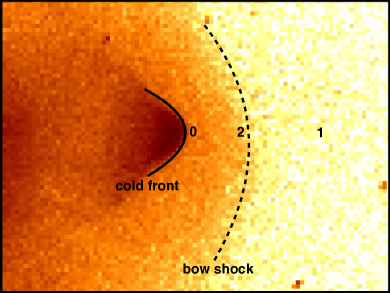
Figure 6: Geometry of flow past a denser and colder region. Here the Bullet cluster is used as a textbook example of cold front and bow shock formations. Zones 0, 1, and 2 are those near the stagnation point, in the undisturbed free stream, and past the bow shock, respectively. While cold fronts may be the result of many different physical events in the cluster, the density discontinuities in them form for the same basic reason: whenever a gas density peak encounters a flow of ambient gas, a contact discontinuity quickly forms.

5 Results

5.1 Masses

Following the approach outlined in Section 4, we obtain $M_{\rm 500,Y_{X}}=(7.14\pm 0.65)\times 10^{14}M_{\odot}$, in very good agreement with the Planck estimated mass of $M_{\rm 500,Y_{SZ}}=(6.59\pm 0.31)\times 10^{14}M_{\odot}$ (Planck Collaboration et al., 2016) despite the merger morphology. This is due to the fact that both $Y_{\rm X}$ and $Y_{\rm SZ}$ are insensitive to the cluster dynamical state (Kravtsov et al., 2006; Sayers et al., 2013). This mass leads to $r_{500}\sim 1.3$ Mpc. We measure $kT=6.5\pm 0.1$ keV within (0.15–1.0) $\times~{}r_{500}$, and a gas mass of $M_{\rm g,500}=(9.7\pm 0.1)\times 10^{13}M_{\odot}$. The gas mass fraction within $r_{500}$ is $f_{\rm g}=0.14\pm 0.01$.

5.2 Images

Figure 2 shows the merged, flat-fielded (vignetting and exposure corrected), and background subtracted $0.5-2$ keV band Chandra ACIS-I image of A3411–12. The image reveals the presence of large scale diffuse emission, which originates from optically-thin thermal plasma with $kT\sim$ 2–8 keV temperature (Section 3).

The distribution of the hot X-ray emitting gas reveals a complex morphology, indicating an active merger history (van Weeren et al., 2013; Giovannini et al., 2013; van Weeren et al., 2017). In particular, the gas distribution is not symmetric, but is elongated in the southeast-northwest direction. In addition, the image shows the presence of sharp surface brightness edges in the central regions of the cluster (see Figure 8).

The above features are characteristic signatures of a merger, which has likely perturbed the hot gas distribution. To explore the nature of these features, and hence, constrain the merger history of the cluster, we derive surface brightness, density, and temperature profiles, which are discussed in the following sections.

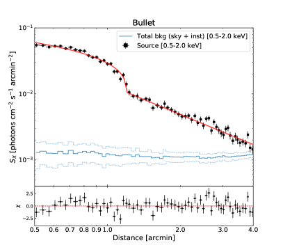
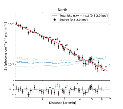
Figure 7: Surface brightness profiles across the northern sector. Left: we present the surface brightness across A3411–12 bullet (cold front). Right: we present the surface brightness further north where a hint of a bow shock is detected. The total background level (i.e. instrumental and astrophysical) is shown by the blue line, with the $\pm 1\sigma$ uncertainties (blue dashed lines). On the bottom of each panel, the residuals (i.e. $\frac{S_{\rm X,obs}-S_{\rm X,mod}}{\Delta S_{\rm X,obs}}$) are displayed.

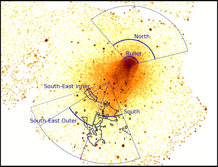
Figure 8: Blue: sectors used for surface brightness extraction. Black: radio contours indicating the location of radio relics. Black contours display the radio emission of A3411–12 at the $3\sigma_{\rm rms}$ level, with $\sigma_{\rm rms}=0.4~{}\mu$Jy beam^-1.

5.3 Temperature, Pressure and Entropy Maps

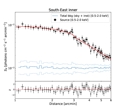
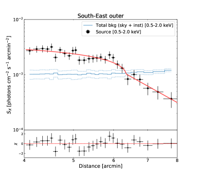
Figure 9: Surface brightness profiles across the southeast sector. Left: we present the surface brightness across A3411–12 southeast. Right: we present the surface brightness further south where a hint of an edge is detected. The total background level (i.e. instrumental and astrophysical) is shown by the blue line, with the $\pm 1\sigma$ uncertainties (blue dashed lines). On the bottom of each panel, the residuals (i.e. $\frac{S_{\rm X,obs}-S_{\rm X,mod}}{\Delta S_{\rm X,obs}}$) are displayed.

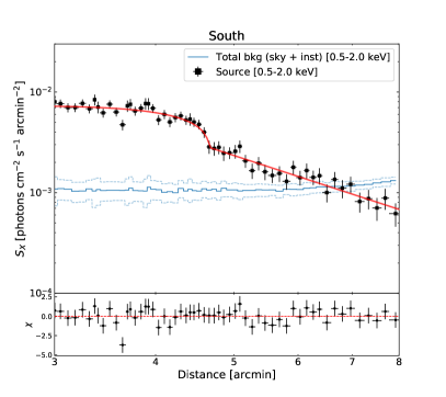
Figure 10: Surface brightness profiles across the south sector. The total background level (i.e. instrumental and astrophysical) is shown by the blue line, with the $\pm 1\sigma$ uncertainties (blue dashed lines). On the bottom of each panel, the residuals (i.e. $\frac{S_{\rm X,obs}-S_{\rm X,mod}}{\Delta S_{\rm X,obs}}$) are displayed.

In this section we present pseudo-density, projected temperature, pseudo-pressure, and pseudo-entropy maps for A3411–12, extracted from the Chandra observations. For typical cluster temperatures (k$T$ = 3 – 10 keV) and metal abundances ($Z$ = 0.1 – 0.5 $Z_{\odot}$), the broadband response of Chandra to optically thin thermal emission from hot gas can be reasonably assumed to be constant with gas temperature. As an example, for a fixed emission measure, the 0.5–2.5 keV count rate of the Chandra ACIS-I declines by only $\sim 17\%$ when $kT$ increases from 4 to 12 keV. Therefore, we can ignore the Chandra response and assume that the count rate per unit volume of the gas is directly proportional to the square of the gas density. Thus, from the surface brightness we can map the projected density of the cluster, and combining that with a temperature map we can also compute the pseudo pressure and entropy maps using the following relations:

$$n_{\rm e}\propto S^{1/2},$$ (8)

$$P=n_{\rm e}kT\propto S^{1/2}T,$$ (9)

$$K=n_{\rm e}^{-2/3}kT\propto S^{-1/3}T,$$ (10)

where $S$ and $T$ are the surface brightness and temperature maps.

We extracted spectra in regions that were created using contbin, an algorithm for binning X-ray data using contours on an adaptively smoothed map. The generated bins closely follow the surface brightness, and are ideal where the surface brightness distribution is not smooth, or the spectral properties are expected to follow the surface brightness (Sanders, 2006). The regions were selected to have a minimum S/N of 50 in the 0.5–7.0 keV band. Background (sky + detector + readout) and exposure maps were used. The temperature map was created by fitting, in the 0.5–7.0 keV band, an absorbed plasma model (XSPEC – wabs*apec) to the spectrum data in each region. NH was fixed to Galactic value of $5.92\times 10^{20}$ (see Section 3.1).

In Figure 5 we present the projected density, temperature, pressure, and entropy maps for A3411. The density and pressure maps present very smooth spatial variations, however the temperature map presents large variations within relatively small distances. The homogeneity of the pressure map across the north surface brightness discontinuity shows that the pressure varies smoothly indicating a cold front, in contrast with shock fronts which present pressure jumps. The entropy map is significantly more homogeneous than the temperature map, especially in the inner regions, suggesting an isentropic process. An isentropic process is the equivalent to the thermodynamic process which is reversible and adiabatic, meaning that no heat is dissipated. This suggests that the merger pushed the low entropy gas back from the core causing it to spread in the downstream, however, in a mild way, so heat dissipation did not happen. On the other hand, the inhomogeneity of the temperature map in the same region suggests that the gas has been mixed.

5.4 Shock and Cold Fronts

For a detailed description of the physics of shock and cold fronts in galaxy clusters, please refer to Markevitch & Vikhlinin (2007); Vikhlinin et al. (2001). Here we discuss briefly the theory behind such phenomena, which will be relevant in the following analysis.

Let us consider a dense and cold gas cloud moving across a hotter gas. In Figure 6, we show an example of this setup. Far upstream from the dense cloud, the gas will be moving (relative to the dense gas cloud) freely. This region is referred to as the free stream and will be labeled with the index 1 (See Figure 6). The hot gas decelerates as it approaches the dense gas cloud, approaching zero velocity at the edge of the dense cloud. This region is referred to as the stagnation point and will be labeled with the index 0. The density discontinuities in cold fronts form whenever a gas density peak encounters a flow of ambient gas, causing a contact discontinuity to quickly form. Furthermore, if the velocity of the dense gas cloud exceeds the sound speed of the hot gas, a bow shock forms at some distance upstream from the dense cloud. The region just inside the bow shock will be indexed as 2 (see Fig. 6 for a visual description of the regions discussed above). The ratio of pressures in the free stream (1) and at the stagnation point (0) is a function of the cloud speed $v$ (Section 114 of Landau & Lifshitz, 1959):

$$\frac{p_{0}}{p_{1}}=\left\{\begin{array}[]{ll}\left(1+\frac{\gamma-1}{2}M_{1}^{2}\right)^{\frac{\gamma}{\gamma-1}},&\mbox{\hskip 2.84544pt $M_{1}\leq 1$}\\ \left(\frac{\gamma+1}{2}\right)^{\frac{\gamma+1}{\gamma-1}}M_{1}^{2}\left(\gamma-\frac{\gamma-1}{2M_{1}^{2}}\right)^{\frac{-1}{\gamma-1}},&\mbox{\hskip 2.84544pt $M_{1}>1$}\\ \end{array}\right.$$ (13)

where $M_{1}=v/c_{1}$ is the Mach number in the free stream and $\gamma$ is the adiabatic index of the gas. The pressure ratio dependence on the square of the Mach number leads to a large increment in the pressure ratio for relatively small changes in the velocity of the cloud, therefore the cloud velocity can be measured rather accurately even if the pressure uncertainties are relatively high.

Table 3: Density jumps and Mach numbers

Sector	$r_{\rm shock}$ (arcmin)	$C$	$M$
Bullet	$1.20^{+0.01}_{-0.03}$	$1.99_{-0.05}^{+0.09}$	cold-front
Northern	$3.48^{+0.61}_{-0.71}$	$1.22_{-0.14}^{+0.20}$	$1.15_{-0.09}^{+0.14}$
Southern	$4.65^{+0.04}_{-0.04}$	$1.70_{-0.09}^{+0.09}$	cold-front
Southeast inner	$3.04^{+0.15}_{-0.18}$	$1.19_{-0.13}^{+0.21}$	$1.13_{-0.08}^{+0.14}$
Southeast outer	$6.34^{+0.40}_{-0.26}$	$1.31_{-0.17}^{+0.22}$	$1.21_{-0.12}^{+0.15}$

Note. — Columns list best fit values for the parameters given by Equations 18 and 19.

Table 4: Temperature

Sector	$r_{\rm in}$ (arcmin)	$r_{\rm out}$ (arcmin)	k$T$ (keV)
N Cold-front	0	1.20	$5.15_{-0.18}^{+0.19}$
N Downstream	1.20	3.48	$7.40_{-0.62}^{+0.62}$
N Upstream	3.48	8	$5.06_{-0.60}^{+0.74}$
S Cold-front	0	4.65	$6.50_{-0.32}^{+0.33}$
S Downstream	4.65	11	$6.40_{-0.96}^{+1.32}$
SE I Downstream	0	3.04	$6.26_{-0.43}^{+0.44}$
SE I Upstream	3.04	11	$4.56_{-0.39}^{+0.43}$
SE O Downstream	0	6.34	$5.81_{-0.39}^{+0.40}$
SE O Upstream	6.34	11	$2.54_{-0.96}^{+1.91}$

Note. — Columns list the sector used to extract the temperature (N – north, S – south, SE I – southeast inner, SE O – southeast outer), the inner and outer radii, and temperature.

As mentioned earlier, if the speed of a blunt body exceeds the speed of sound, a bow shock forms at some distance upstream. The shape of this structure is consistent with an ellipse centered on the center of curvature of the cold front. If the surface brightness discontinuity is interpreted as a shock front, it is straightforward to derive the expected temperature jump, the shock propagation velocity and the velocity of the gas behind the shock, using the Rankine-Hugoniot shock equations (Section 85 of Landau & Lifshitz, 1959):

$$\frac{\rho_{2}}{\rho_{1}} = \frac{(1+\gamma)M_{1}^{2}}{2+(\gamma-1)M_{1}^{2}},$$ (14)

$$\frac{T_{2}}{T_{1}} = \frac{2\gamma M_{1}^{2}-\gamma+1}{\gamma+1}\frac{\rho_{1}}{\rho_{2}}.$$ (15)

where $\rho_{2}/\rho_{1}$ and $T_{2}/T_{1}$ are the ratios of densities and temperatures in the downstream (2) and free stream (1) regions, respectively.

5.4.1 Modeling the density jumps

Following Owers et al. (2009), we can fit the surface brightness profile across a shock assuming spherical symmetry for the gas density profile, which is given by two power laws (broken power law):

$$n(r)=\left\{\begin{array}[]{ll}Cn_{0,2}\left(\frac{r}{r_{\rm shock}}\right)^{-\alpha_{1}},&\mbox{\hskip 25.6073pt $r\leq r_{\rm shock}$}\\ n_{0,2}\left(\frac{r}{r_{\rm shock}}\right)^{-\alpha_{2}},&\mbox{\hskip 25.6073pt $r>r_{\rm shock}$}\\ \end{array}\right.$$ (18)

where $C$ is the density compression ($\rho_{2}/\rho_{1}$), and $r_{\rm shock}$ is the radius at the shock (where the surface brightness discontinuity is located). $C$ is directly related to the Mach number via the Rankine-Hugoniot equations presented in Equation (14). For mono-atomic gas, $\gamma=5/3$, and:

$$C=\frac{4M_{1}^{2}}{3+M_{1}^{2}}.$$ (19)

The gas density at the shock upstream region is typically very low, which makes measuring the temperature jump quite difficult, A3411–12 being no exception despite our very good Chandra data.

5.4.2 Northern Cold and Shock Fronts

Cold fronts are found in many galaxy clusters (Bullet Cluster, A2029, A2204, RXJ1720, Ophiuchus, A2142, A3667, A1644, A520, and many more Markevitch & Vikhlinin, 2007). While cold fronts may be the result of many different physical events in the cluster, the density discontinuities in them form for the same basic reason: whenever a gas density peak encounters a flow of ambient gas, a contact discontinuity quickly forms.

Here, we measure the surface brightness profile in a wedge towards the north of A3411, centered on the bright northern cool core. The left panel of Figure 7 shows the cold front signature, as modeled by a broken power law (Equation 18). The density jump factor is $C=1.99$. The right panel of Figure 7 shows what may be the bow shock, at 2^′.3 upstream from the cold front, modeled as another broken power law. The density jump is $C=1.22_{-0.14}^{+0.20}$, which implies $M=1.15_{-0.09}^{+0.14}$ (with a 90% confidence upper limit of $M<1.6$) if we interpret this density discontinuity as a shock front. We used a Bayesian information criterion (BIC) to compare a single power law model to a broken power law model. For the single power law model, we obtain BIC = 75.9 ($\chi^{2}$ = 67.75). For the broken power law model, we obtain BIC = 75.2 ($\chi^{2}$ = 54.74). Despite the slightly lower BIC in favor of the density jump, no clear conclusion can be drawn from the current data. The density jumps and Mach numbers for all sectors are presented in Table 3.

Table 4 shows the temperature at the regions presented in Figure 8, which are determined by the surface brightness jumps. Towards the north, the cool core becomes very clear in the surface brightness profile, as well as the temperature jump from inside to outside of the stagnation point. Further north, the temperature jump and density discontinuities are only suggestive of a shock front. Indeed, computing the Mach number using temperature (Equation 15) associated with all three suggestive shock fronts (in the Northern, Southeast Inner, and Outer sectors) leads to unconstrained results.

5.4.3 Southeast Radio Relic, Cold Front, and Possible Shock Front

Measuring the surface brightness towards the southeast of A3411–12, we also see the suggestion of an upstream bow shock (right panel of Figure 9).

The surface brightness discontinuity presented in the southeast inner region (see left panel of Figure 9) has been associated with a shock-front, responsible for electron re-acceleration producing the bright radio relic (van Weeren et al., 2017, see also Section 7). For this sector we measure $C=1.19_{-0.13}^{+0.21}$ and $M=1.13_{-0.08}^{+0.14}$ (with a 90% confidence upper limit of $M<1.6$).

5.4.4 Southern Cold Front

Measuring the surface brightness towards the bright X-ray clump in the south of A3411–12, we also see another cold front signature, as the X-ray surface brightness profile is very well modeled by a broken power law (Figure 10). Measuring an upstream bow shock, however, is not possible due to the very low statistic at such a large distance from the cluster X-ray bright regions. For this sector we measure $C=1.70_{-0.09}^{+0.09}$.

6 Merging Scenario

Optical, X-ray, and radio data indicate that A3411–12 is undergoing a major merger. van Weeren et al. (2017) showed that the optical data indicates a clear bimodal galaxy distribution, with velocity dispersion indicating a merger with a 1:1 mass ratio, and a radial velocity difference between the two peaks compatible with zero, suggesting a merger on the plane of the sky. The X-ray data show a bullet-like cool core in the north with extended diffuse X-ray emission in the south, also highly suggestive of a merger happening mostly in the direction south-north on the plane of the sky. Cold fronts in the south and north regions also support this, as well as what seems be a bow shock upstream from the north cold front density discontinuity. Assuming this density discontinuity to be a shock, we measure a Mach number of $M=1.15_{-0.09}^{+0.14}$. The radio data show a large, Mpc scale relic in the south, a typical signature found in the outskirts of many merging clusters.

Thanks to the very good Chandra X-ray data, we are able identify and constrain what seems to be a shock in the south (Southeast Outer sector – it is important to note that we cannot constrain the temperature, therefore the nature of the density jump), with a Mach number of $M=1.21_{-0.12}^{+0.15}$. In van Weeren et al. (2017), the best fit for the density jump at the location of the radio relic gives $M=1.2$, with a 90% confidence upper limit of $M<1.4$, also suggesting a low Mach number. Here we measure at the location of the radio relic presented in van Weeren et al. (2017) (Southeast Inner sector) $M=1.13_{-0.08}^{+0.14}$.

6.1 Merger Analogs

To model the dynamics of the merger we used the method of Wittman (2019), who uses the projected separation, relative line-of-sight velocity, and masses to select analog systems from a cosmological N-body simulation. We followed that work in using the Big Multidark Planck (BigMDPL) Simulation (Klypin et al., 2016) hosted on the cosmosim.org website, but we updated the cluster parameters as follows. First, the X-ray morphology strongly suggests that the subclusters are still outgoing, so we eliminate analog systems that are in the returning phase. Second, our $M_{500}$ estimate implies a total virial mass $\approx 1.4\times M_{500}=10\times 10^{14}$ M_⊙. This is lower than the $16\times 10^{14}$ M_⊙ total mass used by Wittman (2019), who noted that the only available mass estimate available then was a dynamical mass likely to be biased high. Because the velocity dispersions of the two subclusters are almost equal and our X-ray data do not constrain the mass ratio, we search for analog systems with subcluster virial masses of $(5\pm 2.5)\times 10^{14}$ M_⊙.

The resulting constraints are: the subcluster separation vector is $>74$ ($>60$) degrees from the line of sight at 68% (95%) confidence; the time since pericenter passage is 460-790 (340-820) Myr at the same confidence levels; the maximum relative speed reached near pericenter passage, $v_{\rm max}$, is 2000–2500 (1900–2800) $\rm km~{}s^{-1}$; and the relative speed at the time of observation is 540–1100 (320–1400) $\rm km~{}s^{-1}$. Note that the maximum relative speed of the analog halos is likely to be underestimated due to confusion in assigning particles to overlapping halos (Wittman, 2019).

These estimates are consistent with the shock position as follows. Hydrodynamical simulations of a merging cluster (Springel & Farrar, 2007) indicate that shocks are launched from near the center of mass (CM) around the time of pericenter passage. The maximum speed $v_{\rm max}$ sets the speed of the shock front; over time the subclusters slow substantially (and eventually fall back) while the shock slows little. Hence the analogs predict that shock fronts have been traveling at $\gtrsim 1200$ $\rm km~{}s^{-1}$ in CM coordinates for 650 Myr, for a distance of $\gtrsim 830$ kpc. Because the analogs also predict that the separation vector is close to the plane of the sky, we expect the projected separation between shock and CM to be $\gtrsim$ 800 kpc. In fact we find $\sim$ 1.1 Mpc, which indeed requires a projected separation not much less than the physical separation, as well as the analog speed being biased low by several hundred $\rm km~{}s^{-1}$.

If the shock propagates at $\approx 1600$ $\rm km~{}s^{-1}$ in CM coordinates as suggested by the 1.1 Mpc separation, this implies $\approx 3000$ $\rm km~{}s^{-1}$ relative to the unshocked gas, or $\mathcal{M}\approx 3$. The smaller Mach number we find could be due to line-of-sight projections of different parts of the 3-D shock front. It could also be due to slowing of the shock over time: although Springel & Farrar (2007) found that the slowing was only about 10%, their simulations extended only 300 Myr past pericenter, while we are observing A3411 much later, $\approx 650$ Myr after pericenter passage. Addressing these issues will require detailed hydrodynamical simulations, beyond the scope of this paper.

7 Formation of Radio Relics

From our analysis of the density jumps across surface brightness discontinuities we conclude that if they are indeed shocks, they are very mild. However, radio relics extend over Mpcs in the A3411–12 system (see radio emission (red) in Figure 1). The fact that we observe very extended radio relics in a cluster with such low-Mach number shocks is indicative that a population of energetic electrons already existed over extended regions of the cluster.

The southeast inner edge has been discussed in van Weeren et al. (2017) where it is argued that this edge is a shock front where particles from a nearby tailed radio galaxy are being re-accelerated. While there is evidence for a mild density jump at this location, the Chandra data are not deep enough to confirm the presence of a temperature jump. This means that in principle this edge could also trace a cold front. Given that this edge traces a relic, a shock interpretation is more likely, as this has been confirmed for numerous other relics (e.g., van Weeren et al., 2019). However, a cold front (contact discontinuity) might also be able to explain some of the observed radio features. Magnetic field lines are thought to be stretched along the cold front interface (Lyutikov, 2006; Dursi, & Pfrommer, 2008). An alignment of magnetic field might explain the increase of the observed polarization fraction of the radio relic at this location. If the ICM magnetic field is also locally enhanced at the cold front, this will result in a flattening of the radio spectral index, providing that the underlying spectrum contains a spectral cutoff (i.e., is curved). A higher magnetic field strength will then “illuminate” a different part of the underlying electron spectrum, causing the observed spectral index to flatten (Katz-Stone et al., 1993). A curved spectrum with a spectral break is naturally expected due to electron energy losses in the tail of the AGN. Although a shock scenario remains more likely, future temperature measurements will be important to confirm or rule out a cold-front scenario for the origin of the relic.

8 Conclusions

In this paper we presented deep Chandra observations of the merging cluster A3411–12. This remarkable cluster hosts the most compelling evidence for electron re-acceleration at cluster shocks to date. We present gas temperature, X-ray luminosity, gas and total masses, and gas fraction profiles. We computed the shock strength using density jumps to conclude that the Mach number is small ($M\leq 1.15_{-0.09}^{+0.14}$). We also presented pseudo-density, projected temperature, pseudo-pressure, and pseudo-entropy maps. Based on the pseudo-entropy map we conclude that the cluster is undergoing a mild merger, consistent with the small Mach number. On the other hand, radio relics span over Mpcs in the A3411–12 system, which indicates that a population of energetic electrons already existed over extended regions of the cluster. In the southeast of the system there is evidence for a mild density jump, however our Chandra data are not deep enough to confirm the presence of a temperature jump. Therefore, we cannot determine if this edge traces a cold front or a shock. Future higher precision temperature measurements are therefore important to test the shock re-acceleration scenario for radio relic formation.

Appendix A Density jumps and Mach number distributions

Here we present the density jumps and Mach number distributions from Figures 7, 9 and 10. They show the distribution of solutions for the fitted parameters from the X-ray surface brightness profiles across the wedges presented in those figures.

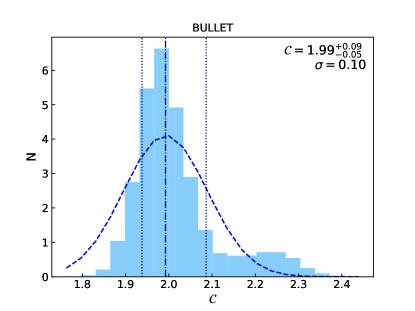
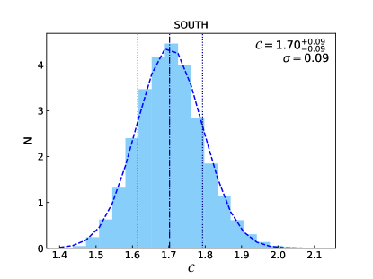
Figure A.1: Distribution of density jumps for the cold fronts in the northern and southern sectors. Left: distribution of density jumps from the MCMC simulations from the cold-front in the northern sector (the bullet). Right: Same as the left panel, except for the southern cold-front.

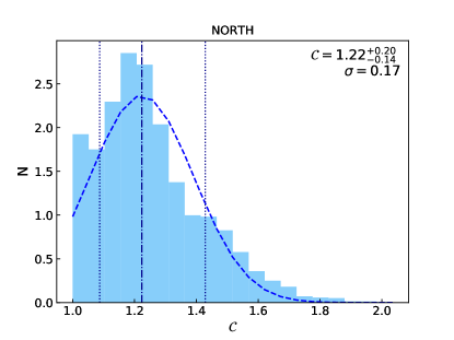
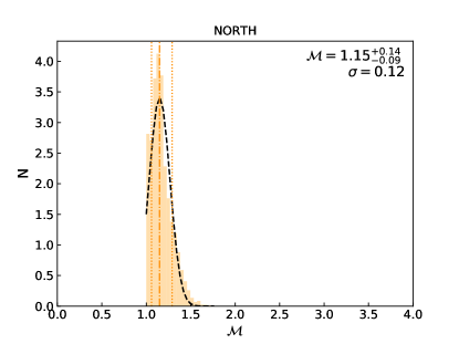
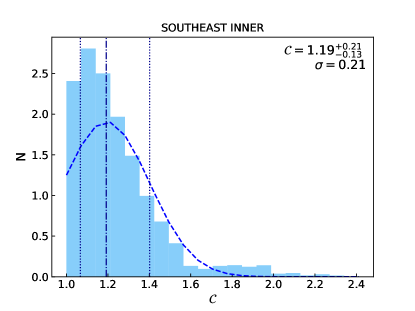
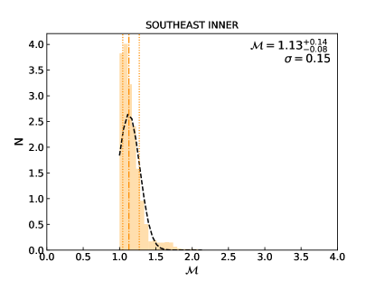
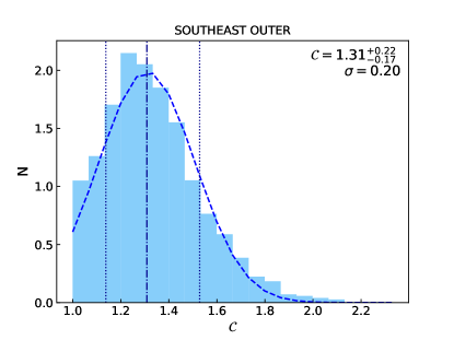
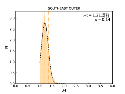
Figure A.2: Distribution of density jumps (left panels) and Mach numbers (right panels) for the discontinuities in the norther and southern sectors. Top panels: distributions of density jumps and Mach numbers from the MCMC simulations from the discontinuity in the northern sector. Center panels: same as top panels, except for the southeast inner sector. Bottom panels: same as top panels, except for the southeast outer sector.

Appendix B MCMC corner plots

Here we present the MCMC “corner plots” (Foreman-Mackey, 2016, 2017) from Figures 7, 9 and 10. They show the distribution of solutions for the fitted parameters from the X-ray surface brightness profiles across the wedges presented in those Figures. For all corner plots, contour levels are drawn at $[0.5,1.0,1.5,2.0]\sigma$ levels.

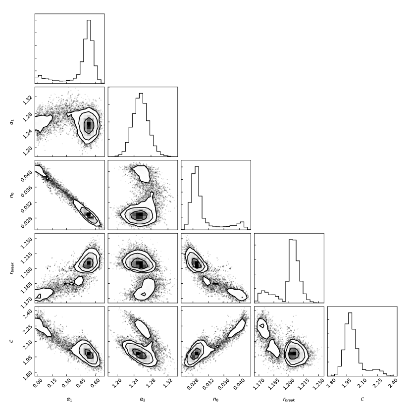
Figure B.1: The MCMC “corner plot” for the distribution of solutions of the fitted parameters from the X-ray surface brightness profiles across the bullet discontinuity (see left panel in Figure 7).

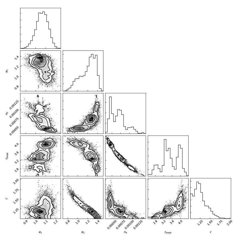
Figure B.2: The MCMC “corner plot” for the distribution of solutions of the fitted parameters from the X-ray surface brightness profiles across the northern discontinuity (see right panel of Figure 7).

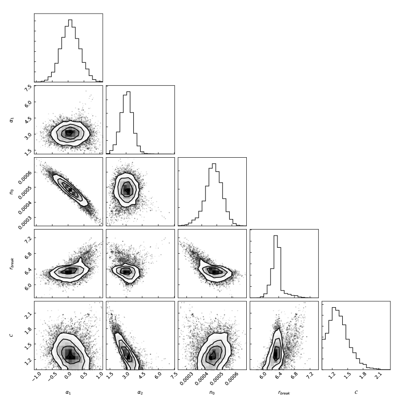
Figure B.3: The MCMC “corner plot” for the distribution of solutions of the fitted parameters from the X-ray surface brightness profiles across the discontinuity in the southeast outer wedge (see left panel in Figure 9).

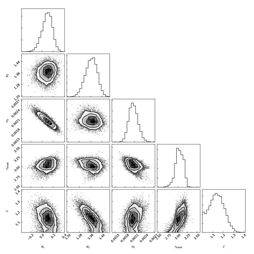
Figure B.4: The MCMC “corner plot” for the distribution of solutions of the fitted parameters from the X-ray surface brightness profiles across the discontinuity in the southeast inner wedge (see top right panel in Figure 9).

Figure B.5: The MCMC “corner plot” for the distribution of solutions of the fitted parameters from the X-ray surface brightness profiles across the discontinuity in the south wedge (see Figure 10).

References

- Anders & Grevesse (1989) Anders, E., & Grevesse, N. 1989, Geochim. Cosmochim. Acta, 53, 197
- Andrade-Santos et al. (2012) Andrade-Santos, F., Lima Neto, G. B., & Laganá, T. F. 2012, ApJ, 746, 139
- Andrade-Santos et al. (2013) Andrade-Santos, F., Nulsen, P. E. J., Kraft, R. P., et al. 2013, ApJ, 766, 107
- Baars et al. (1977) Baars, J. W. M., Genzel, R., Pauliny-Toth, I. I. K., & Witzel, A. 1977, A&A, 61, 99
- Bradač et al. (2006) Bradač, M., Clowe, D., Gonzalez, A. H., et al. 2006, ApJ, 652, 937
- Bradač et al. (2008) Bradač, M., Allen, S. W., Treu, T., et al. 2008, ApJ, 687, 959
- Briggs (1995) Briggs, D. S. 1995, PhD thesis, New Mexico Institute of Mining Technology, Socorro, New Mexico, USA
- Brunetti et al. (2001) Brunetti, G., Setti, G., Feretti, L., & Giovannini, G. 2001, MNRAS, 320, 365
- Buote & Tsai (1996) Buote, D. A., & Tsai, J. C. 1996, ApJ, 458, 27
- Clowe et al. (2004) Clowe, D., Gonzalez, A., & Markevitch, M. 2004, ApJ, 604, 596
- Clowe et al. (2006) Clowe, D., Bradač, M., Gonzalez, A. H., et al. 2006, ApJ, 648, L109
- Dawson et al. (2012) Dawson, W. A., Wittman, D., Jee, M. J., et al. 2012, ApJ, 747, L42
- Dennison (1980) Dennison, B. 1980, ApJ, 239, L93
- Dressler & Shectman (1988) Dressler, A., & Shectman, S. A. 1988, AJ, 95, 985
- Drury (1983) Drury, L. O. 1983, Reports on Progress in Physics, 46, 973
- Dursi, & Pfrommer (2008) Dursi, L. J., & Pfrommer, C. 2008, ApJ, 677, 993.
- Ensslin et al. (1998) Ensslin, T. A., Biermann, P. L., Klein, U., & Kohle, S. 1998, A&A, 332, 395
- Feretti et al. (2012) Feretti, L., Giovannini, G., Govoni, F., & Murgia, M. 2012, A&A Rev., 20, 54
- Finoguenov et al. (2010) Finoguenov, A., Sarazin, C. L., Nakazawa, K., Wik, D. R., & Clarke, T. E. 2010, ApJ, 715, 1143
- Foreman-Mackey (2016) Foreman-Mackey, D. 2016, The Journal of Open Source Software, 1,
- Foreman-Mackey (2017) Foreman-Mackey, D. 2017, Astrophysics Source Code Library, ascl:1702.002
- Giovannini et al. (2013) Giovannini, G., Vacca, V., Girardi, M., et al. 2013, MNRAS, 435, 518
- Giacintucci et al. (2008) Giacintucci, S., Venturi, T., Macario, G., et al. 2008, A&A, 486, 347
- Guo et al. (2014) Guo, X., Sironi, L., & Narayan, R. 2014, ApJ, 794, 153
- Hong et al. (2014) Hong, S. E., Ryu, D., Kang, H., & Cen, R. 2014, ApJ, 785, 133
- Henning et al. (2009) Henning, J. W., Gantner, B., Burns, J. O., & Hallman, E. J. 2009, ApJ, 697, 1597
- Jeltema et al. (2005) Jeltema, T. E., Canizares, C. R., Bautz, M. W., & Buote, D. A. 2005, ApJ, 624, 606
- Jones & Forman (1984) Jones, C., & Forman, W. 1984, ApJ, 276, 38
- Jones & Forman (1999) Jones, C., & Forman, W. 1999, ApJ, 511, 65
- Kang et al. (2007) Kang, H., Ryu, D., Cen, R., & Ostriker, J. P. 2007, ApJ, 669, 729
- Kang & Ryu (2011) Kang, H., & Ryu, D. 2011, ApJ, 734, 18
- Kang et al. (2012) Kang, H., Ryu, D., & Jones, T. W. 2012, ApJ, 756, 97
- Katz-Stone et al. (1993) Katz-Stone, D. M., Rudnick, L., & Anderson, M. C. 1993, ApJ, 407, 549
- Klypin et al. (2016) Klypin, A., Yepes, G., Gottlöber, S., Prada, F., & Heß, S. 2016, MNRAS, 457, 4340
- Kravtsov et al. (2006) Kravtsov, A. V., Vikhlinin, A., & Nagai, D. 2006, ApJ, 650, 128
- Laganá et al. (2008) Laganá, T. F., Lima Neto, G. B., Andrade-Santos, F., & Cypriano, E. S. 2008, A&A, 485, 633
- Laganá et al. (2010) Laganá, T. F., Andrade-Santos, F., & Lima Neto, G. B. 2010, A&A, 511, A15
- Landau & Lifshitz (1959) Landau, L. D., & Lifshitz, E. M. 1959, Course of theoretical physics, Oxford: Pergamon Press, 1959,
- Lyutikov (2006) Lyutikov, M. 2006, MNRAS, 373, 73
- Ma et al. (2010) Ma, C.-J., Ebeling, H., Marshall, P., & Schrabback, T. 2010, MNRAS, 406, 121
- Macario et al. (2011) Macario, G., Markevitch, M., Giacintucci, S., et al. 2011, ApJ, 728, 82
- Markevitch et al. (2002) Markevitch, M., Gonzalez, A. H., David, L., et al. 2002, ApJ, 567, L27
- Markevitch et al. (2005) Markevitch, M., Govoni, F., Brunetti, G., & Jerius, D. 2005, ApJ, 627, 733
- Markevitch & Vikhlinin (2007) Markevitch, M., & Vikhlinin, A. 2007, Phys. Rep., 443, 1
- Mazzotta et al. (2004) Mazzotta, P., Rasia, E., Moscardini, L., & Tormen, G. 2004, MNRAS, 354, 10
- Menanteau et al. (2012) Menanteau, F., Hughes, J. P., Sifón, C., et al. 2012, ApJ, 748, 7
- Mohr et al. (1995) Mohr, J. J., Evrard,
- Ogrean et al. (2013) Ogrean, G. A., Brüggen, M., van Weeren, R. J., et al. 2013, MNRAS, 433, 812
- Ogrean & Brüggen (2013) Ogrean, G. A., & Brüggen, M. 2013, MNRAS, 433, 1701
- Ogrean et al. (2014) Ogrean, G. A., Brüggen, M., van Weeren, R. J., Burgmeier, A., & Simionescu, A. 2014, MNRAS, 443, 2463
- Owers et al. (2009) Owers, M. S., Nulsen, P. E. J., Couch, W. J., & Markevitch, M. 2009, ApJ, 704, 1349
- Petrosian (2001) Petrosian, V. 2001, ApJ, 557, 560
- Planck Collaboration et al. (2011) Planck Collaboration, Ade, P. A. R., Aghanim, N., et al. 2011, A&A, 536, A8
- Planck Collaboration et al. (2016) Planck Collaboration, Ade, P. A. R., Aghanim, N., et al. 2016, A&A, 594, A27
- Randall et al. (2008) Randall, S. W., Markevitch, M., Clowe, D., Gonzalez, A. H., & Bradač, M. 2008, ApJ, 679, 1173-1180
- Russell et al. (2011) Russell, H. R., van Weeren, R. J., Edge, A. C., et al. 2011, MNRAS, 417, L1
- Sanders (2006) Sanders, J. S. 2006, MNRAS, 371, 829
- Sayers et al. (2013) Sayers, J., Czakon, N. G., Mantz, A., et al. 2013, ApJ, 768, 177
- Sobral et al. (2015) Sobral, D., Stroe, A., Dawson, W. A., et al. 2015, MNRAS, 450, 630
- Springel & Farrar (2007) Springel, V., & Farrar, G. R. 2007, MNRAS, 380, 911
- Stroe et al. (2015) Stroe, A., Sobral, D., Dawson, W., et al. 2015, MNRAS, 450, 646
- Stroe et al. (2017) Stroe, A., Sobral, D., Paulino-Afonso, A., et al. 2017, MNRAS, 465, 2916
- Sunyaev & Zeldovich (1972) Sunyaev, R. A., & Zeldovich, Y. B. 1972, Comments on Astrophysics and Space Physics, 4, 173
- van Weeren et al. (2010) van Weeren, R. J., Röttgering, H. J. A., Brüggen, M., & Hoeft, M. 2010, Science, 330, 347
- van Weeren et al. (2012) van Weeren, R. J., Röttgering, H. J. A., Intema, H. T., et al. 2012, A&A, 546, A124
- van Weeren et al. (2013) van Weeren, R. J., Fogarty, K., Jones, C., et al. 2013, ApJ, 769, 101
- van Weeren et al. (2017) van Weeren, R. J., Andrade-Santos, F., Dawson, W. A., et al. 2017, Nature Astronomy, 1, 0005
- van Weeren et al. (2019) van Weeren, R. J., de Gasperin, F., Akamatsu, H., Brüggen, M., Feretti, L., Kang, H., Stroe, A., Zandanel, F. et al. 2019,Space Sci. Rev., 215, 16
- Vikhlinin et al. (2001) Vikhlinin, A., Markevitch, M., & Murray, S. S. 2001, ApJ, 551, 160
- Vikhlinin et al. (2005) Vikhlinin, A., Markevitch, M., Murray, S. S., et al. 2005, ApJ, 628, 655
- Vikhlinin et al. (2006) Vikhlinin, A., Kravtsov, A., Forman, W., et al. 2006, ApJ, 640, 691
- Vikhlinin et al. (2009) Vikhlinin, A., Burenin, R. A., Ebeling, H., et al. 2009, ApJ, 692, 1033
- Wittman (2019) Wittman, D. 2019, arXiv:1905.00375