Exact results for nonequilibrium dynamics in Wigner phase space

Abstract

We study time evolution of Wigner function of an initially interacting one-dimensional quantum gas following the switch-off of the interactions. For the scenario where at $t=0$ the interactions are suddenly suppressed, we derive a relationship between the dynamical Wigner function and its initial value. A two-particle system initially interacting through two different interactions of Dirac delta type is examined. For a system of particles that is suddenly let to move ballistically (without interactions) in a harmonic trap in d dimensions, and using time evolution of one-body density matrix, we derive a relationship between the time dependent Wigner function and its initial value. Using the inverse Wigner transform we obtain, for an initially harmonically trapped noninteracting particles in $d$ dimensions, the scaling law satisfied by the density matrix at time $t$ after a sudden change of the trapping frequency. Finally, the effects of interactions are analyzed in the dynamical Wigner function.

I Introduction

The description of time evolution properties of quantum many body systems is presently a fundamental topic of research. The amazing development of trapping and cooling techniques have led to experimental realization of quantum many-body systems consisting of ultracold atomic gases where atoms are confined in traps Giorgini ; Bloch . These artificial many-body systems can be produced and loaded in various geometric traps. Such experimental progress allowed a full control of the external parameters in the Hamiltonian governing the quantum system dynamics. An interesting issue in the field of ultracold quantum gases is to study the time evolution of a non-equilibrium situation generated through a quantum quench, which consists of a sudden change of the Hamiltonian parameters (for example a change of the harmonic trap frequency or a change in the interaction strength between the atoms of the gas through Feshbach resonance). A quantum quench is the easiest way to drive a system to non-equilibrium: the system is supposed to be in its Hamiltonian ground state until time $t=0$, when the sudden change of a coupling leads to a new Hamiltonian according to which the system evolves for $t>0$. On the theoretical side, significant advances have been carried out in understanding fundamental concepts in the non-equilibrium dynamics of quantum many-body system. Among these ideas is the link between quantum dynamics and quantum chaos Kafri ; Borgonovi and the emergence of a new ensemble in Statistical Mechanics called generalized Gibbs ensemble, which is a more general concept than the usual grand-canonical ensemble and turns out to be a powerful tool in the prediction of relaxation processes for certain integrable one-dimensional systems Rigol ; Rigol2 ; Caux ; Mori ; Eckstein ; Cardy ; Collura .

In the present work we investigate the quantum dynamics of an ultra-cold system of $N$ atoms with equal mass $m$ following an interaction quench from finite to zero interaction strength. We start by writing down the underlying Hamiltonians before and after the interaction quench. For $t<0$ the gas is in equilibrium and its many-body Hamiltonian is

$$H_{0}=\sum\limits_{i=1}^{N}\frac{\mathbf{p}_{i}^{2}}{2m}+\sum_{i=1}^{N}V_{0}(\mathbf{r}_{i})+\frac{1}{2}\sum\limits_{i\neq j}^{N}\sum\limits_{j=1}^{N}v(\mathbf{r}_{i},\mathbf{r}_{j}),$$ (1)

where $\mathbf{p}_{i}=-i\hbar\mathbf{\nabla}_{i}$ is the momentum operator of the particle $i$, $V_{0}$ is an external confining potential, and $v(\mathbf{r}_{i},\mathbf{r}_{j})$ is a two-body atom-atom interaction. We assume that the system is initially in a quantum many-body state $\left|\Phi_{0}\right\rangle$ and its associated initial reduced one-body-density matrix $\rho_{0}(\mathbf{r},\mathbf{r}^{\prime})$ is defined as (see for instance Ref. Dreizler )

$$\rho_{0}(\mathbf{r},\mathbf{r}^{\prime})=N\int d\mathbf{r}_{2}d\mathbf{r}_{3}\cdots d\mathbf{r}_{N}\ \Phi_{0}(\mathbf{r},\mathbf{r}_{2},\mathbf{r}_{3},\dots,\mathbf{r}_{N})\Phi_{0}^{\ast}(\mathbf{r}^{\prime},\mathbf{r}_{2},\mathbf{r}_{3},\dots,\mathbf{r}_{N}).$$ (2)

At $t=0$, the interactions are turned-off and the many-body Hamiltonian is given by

$$H=\sum\limits_{i=1}^{N}\frac{\mathbf{p}_{i}^{2}}{2m}+\sum\limits_{i=1}^{N}V(\mathbf{r}_{i}),$$ (3)

where we are assuming that the external potential may be different before and after the interaction quench. At times $t>0$, the system is in a time dependent quantum state given by

$$\left|\Phi(t)\right\rangle=e^{-\frac{i}{\hbar}Ht}\left|\Phi_{0}\right\rangle.$$ (4)

It should be noted that $\left|\Phi_{0}\right\rangle$ is not an eigenstate of the post-quench Hamiltonian $H$. The latter Hamiltonian describes a system of independent particles, while $\left|\Phi_{0}\right\rangle$ describes the state of an initially interacting particles. Before proceeding further, we shall first derive a relationship between the initial $\rho_{0}(\mathbf{r},\mathbf{r}^{\prime})$, and the time dependent $\rho(\mathbf{r},\mathbf{r}^{\prime};t)$ reduced one-body-density matrices. Using the definition

$$\rho(\mathbf{r},\mathbf{r}^{\prime};t)=N\int d\mathbf{r}_{2}d\mathbf{r}_{3}\dots d\mathbf{r}_{N}\Phi(\mathbf{r},\mathbf{r}_{2},\mathbf{r}_{3},\dots,\mathbf{r}_{N};t)\Phi^{\ast}(\mathbf{r}^{\prime},\mathbf{r}_{2},\mathbf{r}_{3},\dots,\mathbf{r}_{N};t),$$ (5)

we show in Appendix A the following relation

$$\rho(\mathbf{r},\mathbf{r}^{\prime};t)=\int\int U(\mathbf{r},\mathbf{\xi}_{1};t)\rho_{0}(\mathbf{\xi}_{1},\mathbf{\xi}_{2})\,U^{\ast}(\mathbf{r}^{\prime},\mathbf{\xi}_{2};t)\ d\mathbf{\xi}_{1}d\mathbf{\xi}_{2},$$ (6)

where $U(\mathbf{r},\mathbf{\xi}_{1};t)=\left\langle\mathbf{r}\right|e^{-\frac{i}{\hbar}(\frac{\mathbf{p}^{2}}{2m}+V)t}\left|\mathbf{\xi}_{1}\right\rangle$ is the single particle propagator associated to the post quench Hamiltonian in Eq. (3). The above relation describes the time evolution of the one-body density matrix for the considered specific quench of interaction, when the system is suddenly driven from interacting to noninteracting configurations.

Let us now come to our main concern, and study the subsequent dynamics of the system in phase space. For this quench scenario we relate the so-called dynamical Wigner distribution function to its initial value just before the quench. Our interest in the Wigner distribution function Wigner is motivated by the fact that it provides a useful tool to study various properties of many-body systems. Besides, it is well known that it allows a reformulation of quantum mechanics in terms of classical concepts Groenewold ; Moyal ; Gadella0 , and it is also used to generate semi-classical approximations Ozorio ; Brack . Although other distribution functions exist, the Wigner distribution function has the virtue of its mathematical simplicity. Nevertheless, it may take negative values as a manifestation of its quantum nature, and therefore it does not represent a true probability but a quasi-probability distribution Hillery ; Ozorio . Wigner distribution functions have been used in various contexts, as in cold atomic gases Giorgini ; Bloch , quantum optics Walls , quantum information Douce , quantum chaos Berry , and in the study of non-equilibrium dynamics generated by the perturbation of a Fermi gas system Bettelheim . Also, the Wigner distribution function of the noninteracting limit of a Fermi gas system at zero and nonzero temperatures has been the subject of recent studies Dean ; Zyl ; Bencheikh . The Wigner function is defined as the Fourier transform of the one-body density matrix $\rho(\mathbf{r}_{1},\mathbf{r}_{2};t)\equiv\rho(\mathbf{r}+\mathbf{s}/2,\mathbf{r}-\mathbf{s}/2;t)$ on the relative coordinate $\mathbf{s}=\mathbf{r}_{1}-\mathbf{r}_{2}$, where $\mathbf{r}=(\mathbf{r}_{1}+\mathbf{r}_{2})/2$ is the centre of mass coordinate. To be precise, we have in $d$ dimensions

$$W(\mathbf{r},\mathbf{p};t)=\int d\mathbf{s}\,\rho(\mathbf{r}+\mathbf{s}/2,\mathbf{r}-\mathbf{s}/2;t)\,e^{-i\mathbf{p.s}/\hbar},$$ (7)

which is a function of phase space variables $(\mathbf{r},\mathbf{p})$ at time $t$. The inverse transformation reads

$$\rho(\mathbf{r}+\mathbf{s}/2,\mathbf{r}-\mathbf{s}/2;t)=\int\frac{d\mathbf{p}}{(2\pi\hbar)^{d}}\,W(\mathbf{r},\mathbf{p};t)e^{+i\mathbf{p.s}/\hbar}.$$ (8)

Setting $\mathbf{s}=\mathbf{0}$ in Eq. (8), one recovers the spatial local density

$$\rho(\mathbf{r};t):=\rho(\mathbf{r},\mathbf{r};t)=\int\frac{d\mathbf{p}}{(2\pi\hbar)^{d}}\,W(\mathbf{r},\mathbf{p};t),$$ (9)

normalized to the total particle number as $\int\rho(\mathbf{r};t)\,d\mathbf{r}=N$. Integrating $W(\mathbf{r},\mathbf{p};t)$ over the whole space allows to obtain the momentum distribution

$$n(\mathbf{p};t)=\int\frac{d\mathbf{r}}{(2\pi\hbar)^{d}}\,W(\mathbf{r},\mathbf{p};t),\quad\text{such that}\quad\int n(\mathbf{p};t)\,d\mathbf{p}=N.$$ (10)

The structure of the paper is as follows. In Section II we consider the case of an initially untrapped one dimensional interacting system subjected to a sudden swich-off of interactions. The resulting ballistic dynamics is examined in phase space. We derive a relationship between the dynamical Wigner phase space density at time $t>0$ and its initial value before the quench. As an application, we analyze the case of a two-particle system initially interacting through two different zero-range interactions of Dirac delta type. Section III is devoted to a study of nonequilibrium dynamics through the Wigner function of harmonically trapped noninteracting particles. Very recently, this system, in one spatial dimension $(d=1)$, has been the subject of an interesting study DeanEPL , where it is suddenly subjected to a modification of the trapping frequency and a relationship between the resulting time dependent Wigner function and its initial value is obtained. In this section we propose a generalization to arbitrary spatial dimensions $(d\geq 1)$ of this relation by using an alternative fully quantum mechanical method which is based on the use of time evolution of the one-body density matrix. As a bonus, by using the inverse Wigner transformation to our generalized relationship in Wigner phase space, we derive the scaling law of harmonically trapped noninteracting particles in arbitrary dimension $d$, between the one-body density matrix at time $t$ and its initial value. For $d=1$, our result reduces to the one obtained in DeanEPL , as it should.

In order to observe how the dynamical Wigner function following a quench is affected by interactions, we consider physical systems of particles whose dynamics are governed by scaling laws suffering a non-ballistic expansion, and we compare the resulting Wigner function with the one obtained for a ballistic expansion. Some final conclusions put an end to the paper in Section IV.

II Time evolution of Wigner function of an initially untrapped interacting system following a sudden swich-off of interactions.

In this section let us consider the situation where both external potentials $V_{0}$ and $V$ in Eqs. (1) and (3) vanish, and the study is restricted to one-dimensional interacting particles system. The time evolution of the resulting reduced one-body density matrix after a finite time of free expansion $t>0$ is then given by the one dimensional version of Eq. (6), that is

$$\rho(x_{1},x_{2};t)=\int_{-\infty}^{\infty}\int_{-\infty}^{\infty}U(x_{1},\xi_{1};t)\,\rho_{0}(\xi_{1},\xi_{2})\,U^{\ast}(x_{2},\xi_{2};t)\ d\xi_{1}d\xi_{2}.$$ (11)

Here $U(x,\xi;t)=\left\langle x\right|e^{-itH_{0}/\hbar}\left|\xi\right\rangle$ with $H_{0}=-\frac{\hbar^{2}}{2m}\frac{d^{2}}{dx^{2}}$. The matrix element $U(x,\xi;t)$ is the free particle Feynman propagator in the configuration space, given by Feynman

$$U(x,\xi;t)=\sqrt{\frac{m}{2\pi i\hbar t}}\ \exp\left(i\frac{m}{2\hbar t}(x-\xi)^{2}\right).$$ (12)

If we substitute this expression into Eq. (11) we find

$$\rho(x_{1},x_{2};t)=\frac{m}{2\pi\hbar t}\int_{-\infty}^{\infty}\int_{-\infty}^{\infty}e^{i\frac{m}{2\hbar t}\left[(x_{1}-\xi_{1})^{2}-(x_{2}-\xi_{2})^{2}\right]}\rho_{0}(\xi_{1},\xi_{2})\,d\xi_{1}d\xi_{2},$$ (13)

which can be rewritten as

$$\rho(x_{1},x_{2};t)=\frac{m}{2\pi\hbar t}e^{i\frac{m}{2\hbar t}(x_{1}^{2}-x_{2}^{2})}\int_{-\infty}^{\infty}\int_{-\infty}^{\infty}e^{i\frac{m}{2\hbar t}\left[(\xi_{1}-\xi_{2})(\xi_{1}+\xi_{2})-2x_{1}\xi_{1}+2x_{2}\xi_{2})\right]}\rho_{0}(\xi_{1},\xi_{2})\ d\xi_{1}d\xi_{2}.$$ (14)

Now it is more convenient to introduce the center-of-mass and relative coordinates, respectively defined by $z=(\xi_{1}+\xi_{2})/2$ and $z^{\prime}=\xi_{1}-\xi_{2}$. Then we can write

$$\rho(x_{1},x_{2};t)=\frac{m\,e^{i\frac{m}{2\hbar t}(x_{1}^{2}-x_{2}^{2})}}{2\pi\hbar t}\int_{-\infty}^{\infty}\int_{-\infty}^{\infty}e^{i\frac{m}{\hbar t}zz^{\prime}}\,e^{-i\frac{m}{\hbar t}(x_{1}-x_{2})z}\,e^{-i\frac{m}{2\hbar t}(x_{1}+x_{2})z^{\prime}}\,\rho_{0}(z+\tfrac{z^{\prime}}{2},z-\tfrac{z^{\prime}}{2})\,dzdz^{\prime}.$$ (15)

In the following we shall examine the time evolution of the above one-body density matrix in the Wigner representation.

To proceed with computing the Wigner distribution function, we insert Eq. (15) into (7), and we may write

$$W(x,p;t) =\frac{m}{2\pi\hbar t}\int_{-\infty}^{\infty}ds\,e^{i\frac{m}{\hbar t}xs}\int_{-\infty}^{\infty}\int_{-\infty}^{\infty}e^{i\frac{m}{\hbar t}zz^{\prime}}\,e^{-i\frac{m}{\hbar t}zs}\,e^{-i\frac{m}{\hbar t}z^{\prime}x}\,e^{-ips/\hbar}\rho_{0}(z+\tfrac{z^{\prime}}{2},z-\tfrac{z^{\prime}}{2})\,dzdz^{\prime}$$

$$=\frac{m}{2\pi\hbar t}\int_{-\infty}^{\infty}\int_{-\infty}^{\infty}e^{i\frac{m}{\hbar t}zz^{\prime}}\,e^{-i\frac{m}{\hbar t}z^{\prime}x}\,\rho_{0}(z+\tfrac{z^{\prime}}{2},z-\tfrac{z^{\prime}}{2})\,dzdz^{\prime}\int_{-\infty}^{\infty}ds\,e^{\frac{i}{\hbar}\left[\frac{m}{t}x-p-\frac{m}{t}z\right]s}.$$

Carrying out the integration on the variable $s$, we obtain

$$W(x,p;t)=\int_{-\infty}^{\infty}\int_{-\infty}^{\infty}e^{i\frac{m}{\hbar t}zz^{\prime}}e^{-i\frac{m}{\hbar t}xz^{\prime}}\,\delta\left(x-\tfrac{pt}{m}-z\right)\,\rho_{0}(z+\tfrac{z^{\prime}}{2},z-\tfrac{z^{\prime}}{2})\,dzdz^{\prime},$$ (16)

which after integration over $z$ reduces to

$$W(x,p;t)=\int_{-\infty}^{\infty}\rho_{0}(x-\tfrac{pt}{m}+\tfrac{z^{\prime}}{2},x-\tfrac{pt}{m}-\tfrac{z^{\prime}}{2})\,e^{-ipz^{\prime}/\hbar}\,dz^{\prime}.$$ (17)

But according to Eq. (7), the above integral is nothing but the initial Wigner distribution function at $t=0$, and at the phase space point $\left(x-pt/m,p\right)$, so that for $t>0$

$$W(x,p;t)=W_{0}(x-\tfrac{pt}{m},p).$$ (18)

This relation is the Wigner phase space version of Eq. (11). Upon integration over $x$ and making use of the definition in Eq. (10), we get for $t>0$

$$n(p,t)=\int_{-\infty}^{\infty}\frac{dx}{2\pi\hbar}\,W(x,p;t)=\int_{-\infty}^{\infty}\frac{dx}{2\pi\hbar}W_{0}(x-\tfrac{pt}{m},p)=\int_{-\infty}^{\infty}\frac{d\xi}{2\pi\hbar}W_{0}(\xi,p)=n(p,0).$$ (19)

Therefore, we find that under ballistic expansion (where interatomic collisions during the expansion are not present) the dynamical momentum density for $t>0$ is equal to its initial value $n(p,0)$. Some information can be obtained from this result. For example, if one considers an initial quantum gas with short range interaction, whose momentum distribution $n(p,0)$ exhibits a $1/p^{4}$ tail at large momentum (see for instance Ref. Olshanii ), equation (19) says that this long tail behavior is preserved in the dynamical momentum density for all positive times.

It is worth noticing that Eq. (11) remains valid for an initial non-vanishing confining potential $(V_{0}\neq 0)$ provided that one realizes at $t=0$ a simultaneously sudden double quench, where the interactions are turned-off with the release of the trap $(V=0)$. As a consequence the results in Eqs. (18) and (19), in this case hold also true.

II.1 Case of two particles interacting through an attractive $\delta$ interaction

As a first case study we consider a simple model system of two particles interacting through an attractive Dirac delta potential with highly asymmetric mass imbalance: the particle with mass $M$ is so heavy that the center-of-mass motion can be ignored. The problem reduces then to a one-body system and the $m$ mass light particle Hamiltonian is given for $t\leq 0$ by

$$H_{a}=-\frac{\hbar^{2}}{2m}\frac{d^{2}}{dx^{2}}-a\delta(x).$$ (20)

Here $a>0$ is the strength of the interaction. The single normalized bound state is $\phi(x)=\sqrt{\alpha}\,e^{-\alpha\left|x\right|}$ with energy $E_{a}=-ma^{2}/(2\hbar^{2})$, and $\alpha=ma/\hbar^{2}$. The corresponding Wigner distribution function for $t\leq 0$ can be calculated analytically using (7) and is found to be

$$W_{0}(x,p)=\frac{2\alpha^{2}\hbar^{2}\,e^{-2\alpha\left|x\right|}}{p^{2}+\alpha^{2}\hbar^{2}}\left[\cos\left(\frac{2p\left|x\right|}{\hbar}\right)+\frac{\alpha\hbar}{p}\sin\left(\frac{2p\left|x\right|}{\hbar}\right)\right].$$ (21)

A plot of this function is given on the left hand side of Figure 1.

At time $t=0$ the interaction is suddenly turned off ($a=0$) and then, from (18) we get the following Wigner function for $t>0$:

$$W(x,p;t)=\frac{2\alpha^{2}\hbar^{2}\,e^{-2\alpha\left|x-\frac{p}{m}t\right|}}{p^{2}+\alpha^{2}\hbar^{2}}\left[\cos\left(\frac{2p\left|x-\frac{p}{m}t\right|}{\hbar}\right)+\frac{\alpha\hbar}{p}\sin\left(\frac{2p\left|x-\frac{p}{m}t\right|}{\hbar}\right)\right].$$ (22)

A plot of this function $W(x,p;t)$ is given for a particular value of $t>0$ on the right hand side of Figure 1. A clear distortion can be observed as time grows: for $t=0$ there are two symmetry axes, $x=0$ and $p=0$; for bigger values of $t$ the perfect symmetry is lost, although the axes $p=0$ and $p=mx/t$ (this one clockwise rotating with time) play an important role; squeezing is more and more pronounced as $t\to\infty$, the axis $p=mx/t$ approaching the axis $p=0$.

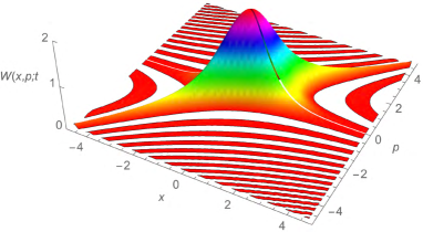
Figure 1: The Wigner function for an attractive Dirac $\delta$ interaction obtained in Eq. (22), for the values $\hbar=m=a=1$. On the left for $t=0$, where two symmetry axes, $x=0$ and $p=0$, are evident; on the right after the quenching, for $t=1$, a clear distortion of the initial function can be appreciated: the perfect symmetry is lost and squeezing appears between the axes $p=0$ and $p=x$. The white regions correspond to small negative values of $W(x,p;t)$.

Finally, using (19) it is easy to show analytically that, the initial momentum density is

$$n(p,0)=\frac{2\alpha^{3}\hbar^{3}}{\pi(p^{2}+\alpha^{2}\hbar^{2})^{2}},$$ (23)

It is easy to check that this result satisfies the second equation in (10) for $N=1$ particle. It has been shown in Olshanii that for a system of zero-range $\delta-$interacting one-dimensional atoms with arbitrary strength, the high-$p$ asymptotic behavior of the momentum distribution for both free and harmonically trapped atoms, exhibits a universal $1/p^{4}$ dependence. As can be seen in Eq. (23) and at large values of the momentum $p$, we recovered this $1/p^{4}$ dependence of the momentum distribution.

II.2 Case of two particles interacting through a $\delta$-$\delta^{\prime}$ interaction

We are going to consider now an extension of the previous study of two interacting particles that takes into account the presence of an extra point-like interaction term in the potential, proportional to $\delta^{\prime}$. This type of point or zero-range potentials are a subject of recent study in differents contexts Gadella1 ; Gadella2 ; Gadella3 ; Romaniega . The Hamiltonian of the light particle with mass $m$ is now given for $t<0$ by

$$H_{a,b}=-\frac{\hbar^{2}}{2m}\frac{d^{2}}{dx^{2}}-a\delta(x)+b\delta^{\prime}(x),\quad a>0,\ b\in\mathbb{R}.$$ (24)

The associated Schrödinger equation has been carefully analyzed in Gadella1 , where it was proven that the above Hamiltonian supports only one bound state of energy

$$E_{a,b}=-\frac{ma^{2}}{2\hbar^{2}\left(1+\frac{m^{2}b^{2}}{\hbar^{4}}\right)^{2}}=-\frac{\hbar^{2}\,\kappa^{2}}{2m},\quad\kappa>0.$$ (25)

The normalized wave function is

$$\phi_{a,b}(x)=A\,e^{-\kappa|x|}\left(1+B\,\text{sign}(x)\right),$$ (26)

where $\text{sign}(x)$ stands for the sign function and

$$A=\frac{\sqrt{ma}}{\hbar(1+B^{2})},\qquad B=\frac{mb}{\hbar^{2}}.$$ (27)

In this case the Wigner distribution function for $t\leq 0$ can be also determined analytically from (7) and it turns out to be the following expression

$$W_{0}(x,p)=\frac{2\kappa^{2}\hbar^{2}\,e^{-2\kappa|x|}}{(1+B^{2})(p^{2}+\kappa^{2}\hbar^{2})} \left[(1-B^{2})\cos\left(\frac{2p\left|x\right|}{\hbar}\right)\right.$$ (28)

$$\qquad\left.+\frac{\kappa^{2}\hbar^{2}+B^{2}(2p^{2}+\kappa^{2}\hbar^{2})+2B(p^{2}+\kappa^{2}\hbar^{2})\,\text{sign}(x)}{\kappa\hbar p}\sin\left(\frac{2p|x|}{\hbar}\right)\right].$$

Remark that the presence of the sign function on (28) indicates the presence of a discontinuity of the Wigner function $W(x,p;0)$ along the line $x=0$. If we consider the limit $B\to 0$ in the last expression we recover the result of equation (21), as one should expect. Some plots of this function are given in Figure 2 for $b=-0.6$, $b=-0.9$, $b=-1.0$ and $b=-1.2$.

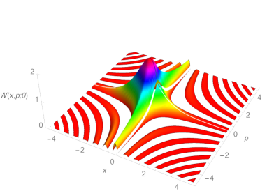
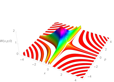
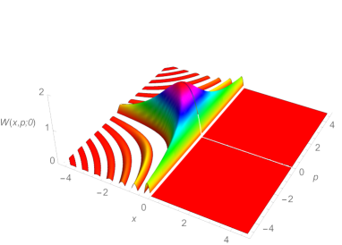
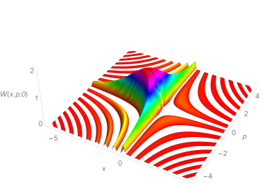
Figure 2: The Wigner function for a Dirac $\delta$-$\delta^{\prime}$ interaction as in (24), for the values $\hbar=m=a=1$. From left to right, and from top to bottom: $b=-0.6$, $b=-0.9$, $b=-1.0$ and $b=-1.2$. The white regions correspond to small negative values of $W_{0}(x,p)$ in (28). The discontinuity of the surface at $x=0$ can be clearly seen on the plots.

At time $t=0$ the interaction is turned off ($a=b=0$) and then, from (18) we get the following Wigner function for $t>0$:

$$W(x,p;t)=\frac{2\kappa^{2}\hbar^{2}\,e^{-2\kappa\left|x-\tfrac{pt}{m}\right|}}{(1+B^{2})(p^{2}+\kappa^{2}\hbar^{2})} \left[(1-B^{2})\cos\left(\frac{2p\left|x-\tfrac{pt}{m}\right|}{\hbar}\right)\right.$$

$$\qquad\left.+\frac{\kappa^{2}\hbar^{2}+B^{2}(2p^{2}+\kappa^{2}\hbar^{2})+2B(p^{2}+\kappa^{2}\hbar^{2})\,\text{sign}(x-\tfrac{pt}{m})}{\kappa\hbar p}\sin\left(\frac{2p|x-\tfrac{pt}{m}|}{\hbar}\right)\right].$$

Plots of this function $W(x,p;t)$ are given in Figure 3 for $t=1$ and values $b=-0.9$ (left) and $b=-1.2$ (right). A clear distortion can be observed comparing with Figure 2: the axis $p=0$ is preserved, but the axis $x=0$ rotates around the origin and becomes $x=p$ (this one changing with time); squeezing is stronger as $t\to\infty$, the axis $x=0$ approaching the axis $p=0$.

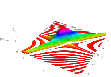
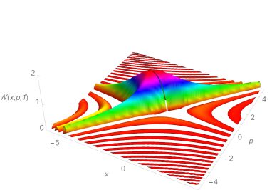
Figure 3: The Wigner function $W(x,p;t=1)$ for a Dirac $\delta$-$\delta^{\prime}$ interaction with values $\hbar=m=a=1$, for $b=-0.9$ (left) and $b=-1.2$ (right), as given by (II.2). Squeezing of the initial function Figure 2 can be appreciated between the axes $p=0$ and $p=x$. The white regions correspond to small negative values of $W(x,p;t=1)$. The discontinuity of the surface at $x=p$ can be clearly seen.

From (19) and (28) the initial momentum density can be determined analytically:

$$n(p,0)=\frac{2\hbar\alpha}{\pi}\ \frac{B^{2}(1+B^{2})^{2}p^{2}+\hbar^{2}\alpha^{2}}{((1+B^{2})^{2}p^{2}+\hbar^{2}\alpha^{2})^{2}}.$$ (30)

Again, it is easy to check that this result satisfies the second equation in (10) for $N=1$ particle. In addition it coincides with (23) in the limit $B=mb/\hbar^{2}\to 0$ and which scales as $1/p^{2}$ for high $p$ if $B\neq 0$ (if $B=0$ it was already mentioned after (23) that it scales as $1/p^{4}$). Hence, it is interesting to observe that the presence of the additional $\delta^{\prime}$ interaction term, changes substantially the high momentum tail of the momentum density: at large values of the momentum $p$, the momentum distribution in Eq. (30) exhibits $1/p^{2}$ behavior while in the absence of $\delta^{\prime}$ interaction this density scales as $1/p^{4}$. A plot of the momentum density as a function of $p$ and $B$ in Figure 4 clearly shows two effects. The aforementioned behavior at large values of $p$ and the appearance of a local minimum around $p=0$. This minimum is due to the presence of a polynomial in the numerator of the expression of $n(p)$ generated by the additional $\delta^{\prime}$ interaction term. We observe that this minimum is more pronounced as $B$ increases and transforms to a maximum for smaller $B$ values. To be more precise, the point $p=0$ is a minimum of $n(p)$ for $B^{2}>2$ and a maximum otherwise. In addition, if $B^{2}>2$ two symmetrical maxima appear at the points

$$p=\pm\frac{\hbar\alpha\sqrt{B^{2}-2}}{B(1+B^{2})}.$$

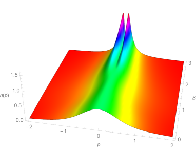
Figure 4: Momentum density $n(p)$ as given by (30) as a function of $p$ and $B\geq 0$, with values $\hbar=m=a=1$. For $B=0$ we recover the profile of (23), which is similar for $B^{2}\leq 2$. For values such that $B^{2}>2$ a peculiar structure appears around $p=0$: $p=0$ turns from a maximum to a minimum and two symmetrical maxima appear at the points $p=\pm\hbar\alpha\sqrt{B^{2}-2}/(B(1+B^{2}))$.

III Time evolution of Wigner distribution function following a sudden change of trapping harmonic potential in d dimensions

Very recently Dean et al. DeanEPL computed the time evolution of the Wigner function $W(x,p;t)$ for a one-dimensional system of noninteracting fermions (called also system of independent fermions), initially trapped by a harmonic oscillator potential with frequency $\omega_{0}$, subjected to a sudden change of frequency passing from $\omega_{0}$ to $\omega$. At time $t$, after this quench it was found (see Eq. (13) of DeanEPL ) that

$$W(x,p;t)=W_{0}\left(x\cos\omega t-\frac{p\sin\omega t}{m\omega},m\omega x\sin\omega t+p\cos\omega t\right),$$ (31)

where $W_{0}$ is the initial Wigner function of the system. To derive this relationship the Liouville equation is used. Here we propose an alternative fully quantum mechanical derivation based on the use of time evolution of one-body density matrix which is valid for an arbitrary spatial dimension $d$, which obviously reduces to the result in (31) for $d=1$ as it should.

Consider a system of noninteracting fermions initially confined in a $d-$dimensional isotropic harmonic oscillator potential of the form $V_{0}(\mathbf{r})=m\omega_{0}^{2}\mathbf{r}^{2}/2$. Suddenly the frequency is changed from $\omega_{0}$ to $\omega$ and the system expands in the potential $V(\mathbf{r})=m\omega^{2}\mathbf{r}^{2}/2$. According to (6), the time evolution of the resulting one-body density matrix at $t>0$ is then given by

$$\rho(\mathbf{r}_{1},\mathbf{r}_{2};t)=\int\int U_{osc}(\mathbf{r}_{1},\mathbf{\xi}_{1};t)\rho_{0}(\mathbf{\xi}_{1},\mathbf{\xi}_{2})\,U_{osc}^{\ast}(\mathbf{r}_{2},\mathbf{\xi}_{2};t)\ d\mathbf{\xi}_{1}d\mathbf{\xi}_{2},$$ (32)

Here $\rho_{0}(\mathbf{\xi}_{1},\mathbf{\xi}_{2})$ is the one-body density matrix at $t=0$  and $U_{osc}(\mathbf{r}_{1},\mathbf{\xi}_{1};t)$ is the well known propagator associated to the isotropic harmonic oscillator potential with frequency $\omega$, given in $d$ dimensions by Feynman

$$U_{osc}(\mathbf{r}_{1},\mathbf{\xi}_{1};t)=\left(\frac{m\omega}{2\pi i\hbar\sin\omega t}\right)^{\frac{d}{2}}\exp\left[i\frac{m\omega}{2\hbar\sin\omega t}[(\mathbf{r}_{1}^{2}+\mathbf{\xi}_{1}^{2})\cos\omega t-2\mathbf{r}_{1}\mathbf{\cdot\mathbf{\xi}_{1}}]\right]$$ (33)

by substitution we obtain

$$\rho(\mathbf{r}_{1},\mathbf{r}_{2};t)=\left(\frac{m\omega}{2\pi\hbar\left|\sin\omega t\right|}\right)^{d}\int\int\rho_{0}(\mathbf{\xi}_{1},\mathbf{\xi}_{2})e^{\frac{im\omega}{2\hbar\sin\omega t}[(\mathbf{r}_{1}^{2}+\mathbf{\xi}_{1}^{2}-\mathbf{r}_{2}^{2}-\mathbf{\xi}_{2}^{2})\cos\omega t-2\mathbf{r}_{1}\mathbf{.\mathbf{\xi}_{1}}+2\mathbf{r}_{2}\cdot\mathbf{\mathbf{\xi}_{2}}]}d\mathbf{\xi}_{1}d\mathbf{\xi}_{2}.$$

Using the centre of mass $\mathbf{u}=(\mathbf{\xi}_{1}+\mathbf{\xi}_{2})/2$ and relative $\mathbf{v}=(\mathbf{\xi}_{1}-\mathbf{\xi}_{2})$ coordinates we can write

$$\rho(\mathbf{r}_{1},\mathbf{r}_{2};t) = \left(\frac{m\omega}{2\pi\hbar\left|\sin\omega t\right|}\right)^{d}e^{i\frac{m\omega\cos\omega t}{2\hbar\sin\omega t}(\mathbf{r}_{1}^{2}-\mathbf{r}_{2}^{2})}\int\int\rho_{0}\left(\mathbf{u+}\frac{\mathbf{v}}{2},\mathbf{u-}\frac{\mathbf{v}}{2}\right)e^{\frac{im\omega}{2\hbar\sin\omega t}[(2\mathbf{u}\cos\omega t-(\mathbf{r}_{1}+\mathbf{r}_{2})).\mathbf{v}-2\mathbf{u.}(\mathbf{r}_{1}-\mathbf{r}_{2})]}\ d\mathbf{u}d\mathbf{v.}$$

According to the definition in Eq. (7), the Wigner function of this density matrix can be written as

$$W(\mathbf{r},\mathbf{p};t)=\left(\frac{m\omega}{2\pi\hbar\left|\sin\omega t\right|}\right)^{d}\int\int e^{\frac{im\omega}{\hbar\sin\omega t}(\mathbf{u}\cos(\omega t)-\mathbf{r})\mathbf{v}}\rho_{0}\left(\mathbf{u+}\frac{\mathbf{v}}{2},\mathbf{u-}\frac{\mathbf{v}}{2}\right)\,d\mathbf{u}d\mathbf{v}\int e^{\frac{i}{\hbar}\left(m\omega\mathbf{r}\cot g(\omega t)-\frac{m\omega}{\sin\omega t}\mathbf{u}-\mathbf{p}\right).\mathbf{s}}\,d\mathbf{s},$$ (34)

with $\mathbf{r}=(\mathbf{r}_{1}+\mathbf{r}_{2})/2$ and $\mathbf{s}=\mathbf{r}_{1}-\mathbf{r}_{2}$. We can perform the $d$ dimensional $\mathbf{s}$ integration,

$$\int e^{\frac{i}{\hbar}\left(m\omega\mathbf{r}\cot g(\omega t)-\frac{m\omega}{\sin\omega t}\mathbf{u}-\mathbf{p}\right).\mathbf{s}}\,d\mathbf{s} = \left(2\pi\right)^{d}\delta\left(\frac{m\omega}{\hbar}\mathbf{r}\cot g(\omega t)-\frac{m\omega}{\hbar\sin\omega t}\mathbf{u}-\frac{\mathbf{p}}{\hbar}\right)$$ (35)

$$= \left(2\pi\hbar\right)^{d}\left(\frac{\left|\sin\omega t\right|}{m\omega}\right)^{d}\delta\left(\mathbf{r}\cos\omega t-\mathbf{u}-\frac{\sin\omega t}{m\omega}\mathbf{p}\right)$$

where we have used the property $\delta(a\mathbf{b})=\delta(\mathbf{b})/\left|a\right|^{d}$, and therefore Eq. (34) reduces to

$$W(\mathbf{r},\mathbf{p};t)=\int\int e^{\frac{im\omega}{\hbar\sin\omega t}(\mathbf{u}\cos(\omega t)-\mathbf{r})\mathbf{v}}\rho_{0}\left(\mathbf{u+}\frac{\mathbf{v}}{2},\mathbf{u-}\frac{\mathbf{v}}{2}\right)\delta\left(\mathbf{r}\cos\omega t-\mathbf{u}-\frac{\sin\omega t}{m\omega}\mathbf{p}\right)\,d\mathbf{u}d\mathbf{v}.$$

After $\mathbf{u}$-integration, we get

$$W(\mathbf{r},\mathbf{p};t)=\int e^{-\frac{i}{\hbar}\left[m\omega\mathbf{r}\sin\omega t+\mathbf{p}\cos\omega t\right].\mathbf{v}}\rho_{0}\left(\mathbf{r}\cos\omega t-\frac{\sin\omega t}{m\omega}\mathbf{p+}\frac{\mathbf{v}}{2},\mathbf{r}\cos\omega t-\frac{\sin\omega t}{m\omega}\mathbf{p-}\frac{\mathbf{v}}{2}\right)\,d\mathbf{v}.$$

Notice that according to Eq. (7), the above expression represents the initial Wigner function at a multidimensional phase space point $\left(\mathbf{r}\cos\omega t-\frac{\mathbf{p}\sin\omega t}{m\omega},m\omega\mathbf{r}\sin\omega t+\mathbf{p}\cos\omega t\right)$, that is

$$W(\mathbf{r},\mathbf{p};t)=W_{0}\left(\mathbf{r}\cos\omega t-\frac{\mathbf{p}\sin\omega t}{m\omega},m\omega\mathbf{r}\sin\omega t+\mathbf{p}\cos\omega t\right),$$ (36)

which ends the proof and reduces to the result given in Eq. (31) for $d=1$. Notice that if $\omega\rightarrow 0$, this relation reduces to the result given in Eq. (18), as it should.

The existence of alternative derivations for a given problem can enrich one’s insight in solving other problems related to it. In this respect, it is interesting to see how our generalized phase space result translates in a real space. In other words, what is the relation between the one-body density matrix $\rho(\mathbf{r}_{1},\mathbf{r}_{2};t)$ at time $t$ and its initial value $\rho_{0}(\mathbf{r}_{1},\mathbf{r}_{2})$ at $t=0$ in $d$ dimensions. To obtain this connection, we shall directly apply the inverse Wigner transformation to both sides of Eq. (8) with (36), we obtain the one-body density matrix in real space at time $t$

$$\rho(\mathbf{r}+\mathbf{s}/2,\mathbf{r}-\mathbf{s}/2;t)=\int\frac{d\mathbf{p}}{(2\pi\hbar)^{d}}\,W_{0}\left(\mathbf{r}\cos\omega t-\frac{\mathbf{p}\sin\omega t}{m\omega},m\omega\mathbf{r}\sin\omega t+\mathbf{p}\cos\omega t\right)e^{i\mathbf{p\cdot s}/\hbar}.$$ (37)

Although the analytical expression of $W_{0}$ in $d=1$ is known to be given in terms of Laguerre polynomials $L_{k}$ for arbitrary $N$ Hillery as

$$W_{0}\left(x,p\right)=2\exp\left\{-\frac{2}{\hbar\omega_{0}}\left(\frac{p^{2}}{2m}+\frac{1}{2}m\omega_{0}^{2}x^{2}\right)\sum_{k=0}^{N-1}(-1)^{k}L_{k}\left(\frac{4}{\hbar\omega_{0}}\left(\frac{p^{2}}{2m}+\frac{1}{2}m\omega_{0}^{2}{x}^{2}\right)\right)\right\},$$

and its expression in $d$ dimensions can be shown to be given in terms of generalized Laguerre polynomials $L_{k}^{(d-1)}$ Zyl ,

$$W_{0}(\mathbf{r},\mathbf{p})=2^{d}\exp\left\{-\frac{2}{\hbar\omega_{0}}\left(\frac{\mathbf{p}^{2}}{2m}+\frac{1}{2}m\omega_{0}^{2}\mathbf{r}^{2}\right)\sum_{k=0}^{N-1}(-1)^{k}L_{k}^{(d-1)}\left(\frac{4}{\hbar\omega_{0}}\left(\frac{\mathbf{p}^{2}}{2m}+\frac{1}{2}m\omega_{0}^{2}\mathbf{r}^{2}\right)\right)\right\},$$ (38)

here its use to calculate the integral in Eq. (37) is not straightforward.

Alternatively, we propose to use expression of the so-called Bloch propagator in Wigner phase space which is related to the density operator through an appropriate Laplace transform. This relation is obtained as follows. For a system of $N$  noninteracting fermions moving in a potential $V(\mathbf{r})$, the one-body density matrix is

$$\rho_{0}(\mathbf{r}_{1},\mathbf{r}_{2})=\sum_{k}\phi_{k}(\mathbf{r}_{1})\phi_{k}^{\ast}(\mathbf{r}_{2})\theta(\mu-\varepsilon_{k}),$$

where the sum is over occupied single-particle states up to the Fermi energy $\mu$, and the $\phi_{k}$’s and $\varepsilon_{k}$’s are respectively the normalized single particle wavefunctions and their corresponding energies, that is $H_{0}\phi_{k}=\varepsilon_{k}\phi_{k}$. The Heaviside unit-step function is denoted by $\theta(x)$ and by using the inverse Laplace transform identity Abramowitz

$$\theta(\mu-\varepsilon_{k})=\int_{c-i\infty}^{c+i\infty}\frac{dz}{2\pi i}\frac{e^{z(\mu-\varepsilon_{k})}}{z},$$

we can write the density matrix $\rho_{0}(\mathbf{r}_{1},\mathbf{r}_{2})$ as an inverse Laplace transformation (see Brack and references quoted therein), so that

$$\rho_{0}(\mathbf{r}_{1},\mathbf{r}_{2})=\int\limits_{c-i\infty}^{c+i\infty}\frac{dz}{2\pi i}\ e^{z\mu}\ \frac{C_{0}(\mathbf{r}_{1},\mathbf{r}_{2};z)}{z},$$ (39)

with $C_{0}(\mathbf{r}_{1},\mathbf{r}_{2};z)=\sum_{k}\phi_{k}(\mathbf{r}_{1})\phi_{k}^{\ast}(\mathbf{r}_{2})e^{-z\varepsilon_{k}}$ the matrix elements of the Bloch operator $e^{-zH_{0}}$. Here the parameter $z$ is considered as a mathematical variable which in general is taken to be complex and $c$ is a positive constant. We can immediately obtain the desired relation by writing the Wigner phase space version of Eq. (39) so that

$$W_{0}(\mathbf{r},\mathbf{p})=\int\limits_{c-i\infty}^{c+i\infty}\frac{dz}{2\pi i}\ e^{z\mu}\ \frac{\widetilde{C}_{0}(\mathbf{r},\mathbf{p;}z)}{z},$$ (40)

where $\widetilde{C}_{0}(\mathbf{r},\mathbf{p;}z)$ denotes the Wigner transform of $C_{0}(\mathbf{r}_{1},\mathbf{r}_{2};z)$. For the case of an isotropic harmonic potential in $d$ dimensions, the phase space function $\widetilde{C}_{0}(\mathbf{r},\mathbf{p;}z)$ has a simple explicit expression Hillery ; Ozorio ,

$$\widetilde{C}_{0}(\mathbf{r},\mathbf{p;}z)=\frac{1}{\left[\cosh\left(\frac{z\hbar\omega_{0}}{2}\right)\right]^{d}}e^{-\frac{2}{\hbar\omega_{0}}\left(\tanh\frac{z\hbar\omega_{0}}{2}\right)\left(\frac{\mathbf{p}^{2}}{2m}+\frac{1}{2}m\omega_{0}^{2}\mathbf{r}^{2}\right)}.$$ (41)

To end these preparations, we give the expression of the inverse Wigner transform of Eq. (41), in terms of centre of mass and relative coordinates (see BencheikhJPA and references quoted therein),

$$C_{0}(\mathbf{r}+\mathbf{s}/2,\mathbf{r}-\mathbf{s}/2)=\left(\frac{m\omega}{2\pi\hbar\sinh z\hbar\omega}\right)^{\frac{d}{2}}e^{-\frac{m\omega}{\hbar}\left[\mathbf{r}^{2}\tanh\left(\frac{z\hbar\omega}{2}\right)+\frac{\mathbf{s}^{2}}{4}\text{coth}\left(\frac{z\hbar\omega}{2}\right)\right]},$$ (42)

an expression which will be used shortly.

Now we are in position to proceed with the integral in Eq. (37). Let us substitute Eq. (40) into  (37), we obtain

$$\rho(\mathbf{r}+\tfrac{\mathbf{s}}{2},\mathbf{r}-\tfrac{\mathbf{s}}{2};t)=\int\limits_{c-i\infty}^{c+i\infty}\frac{dz}{2\pi i}\frac{e^{z\mu}}{z}\int\frac{d\mathbf{p}}{(2\pi\hbar)^{d}}e^{i\frac{\mathbf{p\cdot s}}{\hbar}}\widetilde{C}_{0}\left(\mathbf{r}\cos\omega t-\frac{\mathbf{p}\sin\omega t}{m\omega},m\omega\mathbf{r}\sin\omega t+\mathbf{p}\cos\omega t;z\right),$$ (43)

and using the expression of $\widetilde{C}_{0}$ in Eq. (41), we get

$$\rho(\mathbf{r}+\mathbf{s}/2,\mathbf{r}-\mathbf{s}/2;t) = \int\limits_{c-i\infty}^{c+i\infty}\frac{dz}{2\pi i}\frac{e^{z\mu}}{z\left[\cosh\left(\frac{z\hbar\omega_{0}}{2}\right)\right]^{d}}\int\frac{d\mathbf{p}}{(2\pi\hbar)^{d}}e^{i\frac{\mathbf{p\cdot s}}{\hbar}}$$ (44)

$$\qquad\qquad\times\left[e^{-\frac{2}{\hbar\omega_{0}}\left(\tanh\frac{z\hbar\omega_{0}}{2}\right)\left(\frac{\left(m\omega\mathbf{r}\sin\omega t+\mathbf{p}\cos\omega t\right)^{2}}{2m}+\frac{1}{2}m\omega_{0}^{2}\left(\mathbf{r}\cos\omega t-\frac{\mathbf{p}\sin\omega t}{m\omega}\right)^{2}\right)}\right].$$

The above integral on $\mathbf{p}$ is carried out in the Appendix B, and therefore we have

$$\rho(\mathbf{r}+\tfrac{\mathbf{s}}{2},\mathbf{r}-\tfrac{\mathbf{s}}{2};t)=\frac{e^{i\frac{m}{\hbar}\frac{\dot{b}(t)}{b(t)}\mathbf{r}\cdot\mathbf{s}}}{(b(t))^{d}}\int\limits_{c-i\infty}^{c+i\infty}\frac{dz}{2\pi i}\frac{e^{z\mu}}{z}\left(\frac{m\omega_{0}\text{ }}{2\pi\sinh z\hbar\omega_{0}}\right)^{\frac{d}{2}}e^{-\frac{m\omega}{\hbar}\left[\frac{\mathbf{r}^{2}}{b^{2}}\tanh\left(\frac{z\hbar\omega}{2}\right)+\frac{\mathbf{s}^{2}}{4b^{2}}\text{coth}\left(\frac{z\hbar\omega}{2}\right)\right]},$$ (45)

where $b(t)$ is a time dependent scaling factor given by

$$b(t)=\sqrt{1+\left(\frac{\omega_{0}^{2}}{\omega^{2}}-1\right)\sin^{2}\omega t},$$ (46)

which is the solution of $\dot{b}(t)=\left(\frac{\omega_{0}^{2}}{\omega^{2}}-1\right)\left(\omega\sin\omega t\cos\omega t\right)/b(t)$. Equation (42) allows us to write Eq. (45) as

$$\rho(\mathbf{r}+\mathbf{s}/2,\mathbf{r}-\mathbf{s}/2;t)=\frac{e^{i\frac{m}{\hbar}\frac{\dot{b}(t)}{b(t)}\mathbf{r}\cdot\mathbf{s}}}{(b(t))^{d}}\int\limits_{c-i\infty}^{c+i\infty}\frac{dz}{2\pi i}\ \frac{e^{z\mu}}{z}\ C_{0}\left(\frac{\mathbf{r}}{b(t)}+\frac{\mathbf{s}}{2b(t)},\frac{\mathbf{r}}{b(t)}-\frac{\mathbf{s}}{2b(t)}\right).$$ (47)

We observe that the above inverse Laplace transform is nothing but the initial one-body density matrix at rescaled positions, with $b(t)$ as the scaling factor. We then arrive to

$$\rho(\mathbf{r}+\mathbf{s}/2,\mathbf{r}-\mathbf{s}/2;t)=\frac{e^{i\frac{m}{\hbar}\frac{\dot{b}(t)}{b(t)}\mathbf{r}\cdot\mathbf{s}}}{(b(t))^{d}}\ \rho_{0}\left(\frac{\mathbf{r}}{b(t)}+\frac{\mathbf{s}}{2b(t)},\frac{\mathbf{r}}{b(t)}-\frac{\mathbf{s}}{2b(t)}\right),$$ (48)

returning to the original coordinates, $\mathbf{r}_{1}=$ $\mathbf{r}+\mathbf{s}/2$, $\mathbf{r}_{2}=$ $\mathbf{r}-\mathbf{s}/2$, and since $\mathbf{r}\cdot\mathbf{s=(r}_{1}^{2}-\mathbf{r}_{2}^{2})/2$, the above scaling law becomes

$$\rho(\mathbf{r}_{1},\mathbf{r}_{2};t)=\frac{e^{i\frac{m}{2\hbar}\frac{\dot{b}(t)}{b(t)}\mathbf{(r}_{1}^{2}-\mathbf{r}_{2}^{2})}}{(b(t))^{d}}\ \rho_{0}\left(\frac{\mathbf{r}_{1}}{b(t)},\frac{\mathbf{r}_{2}}{b(t)}\right),$$ (49)

a result valid for arbitrary dimensions. For $d=1$, one recovers the result obtained by the rescaling method DeanEPL .

III.1 Ballistic versus non-ballistic expansions in phase space

It is important to note that the above scaling law obtained for trap to trap quench is not restricted just to noninteracting particles. In fact, the scaling law in Eq. (49) was proven to hold also for some physical systems of interacting particles in which the interactions are acting before and after the quench of the harmonic potential (non ballistic expansion). This is the case for the two following situations: (i) the Tonks-Girardeau gas, which consists in a gas of identical bosons interacting through very strong repulsive zero-range interactions, confined by harmonic trap in one dimension $(d=1)$ Minguzzi ; Ruggiero , and (ii) for harmonically trapped interacting fermions in three dimensions $(d=3)$ at unitarity Castin . Notice that long time ago Pitaevskii and Rosch PitaevskiiRosch introduced a scaling ansatz for a two dimensional bosonic system of particles interacting with contact or inverse square interaction. Later on, scaling approach to quantum non-equilibrium dynamics of interacting systems subject to external linear and parabolic potentials has been examined in Gritsev , where many-body scaling solutions to more general types of interaction and arbitrary dimensionality where obtained.

It may be of interest to see how the above scaling law is expressed in Wigner phase space. For obtaining this result, we substitute Eq. (48) into  (7) and we obtain

$$W(\mathbf{r},\mathbf{p};t) = \frac{1}{(b(t))^{d}}\int d\mathbf{s}\ \rho_{0}\left(\frac{\mathbf{r}}{b(t)}+\frac{\mathbf{s}}{2b(t)},\frac{\mathbf{r}}{b(t)}-\frac{\mathbf{s}}{2b(t)}\right)\,e^{-\frac{i}{\hbar}\left(b(t)\mathbf{p-}m\dot{b}(t)\mathbf{r}\right)\cdot\frac{\mathbf{s}}{b(t)}}$$ (50)

$$= \int d\mathbf{u}\ \rho_{0}\left(\frac{\mathbf{r}}{b(t)}+\frac{\mathbf{u}}{2},\frac{\mathbf{r}}{b(t)}-\frac{\mathbf{u}}{2}\right)\,e^{-\frac{i}{\hbar}\left(b(t)\mathbf{p-}m\dot{b}(t)\mathbf{r}\right)\cdot\mathbf{\mathbf{u}}},$$

and according to Eq. (7), the right-hand side represent the initial Wigner function at phase space point $\left(\frac{\mathbf{r}}{b(t)},b(t)\mathbf{p-}m\dot{b}(t)\mathbf{r}\right)$, so that

$$W(\mathbf{r},\mathbf{p};t)=W_{0}\left(\frac{\mathbf{r}}{b(t)},b(t)\mathbf{p-}m\dot{b}(t)\mathbf{r}\right),$$ (51)

where we recall that $b(t)$ is given by (46).

As stated for Eq. (49), it follows that the relation in Eq. (51) is not only valid for noninteracting particle systems but also for the above two systems pertaining to interacting particles. The interested reader may ask on the difference between Wigner functions given respectively by Eq. (36) and (51). The time dependent Wigner function in Eq. (36) describes a ballistic expansion (interactions are suppressed) following the quench of the harmonic potential while the Wigner function in Eq. (51) concerns ballistic or a nonballistic expansion after the quench of the harmonic trap pertaining to the nature (interacting or noninteracting) of the initially confined system before the quench. We can show that for an initially harmonically confined noninteracting particle system subjected to a quench of the potential, the two forms Eq. (36) and (51) are identical, that is

$$W_{0}\left(\mathbf{r}\cos\omega t-\frac{\mathbf{p}\sin\omega t}{m\omega},m\omega\mathbf{r}\sin\omega t+\mathbf{p}\cos\omega t\right)=W_{0}\left(\frac{\mathbf{r}}{b(t)},b\mathbf{p-}m\dot{b}(t)\mathbf{r}\right).$$ (52)

In fact for a system of $N$ noninteracting fermions confined in a $d$ dimensional isotropic harmonic potential with frequency $\omega_{0}$, the Wigner function was given in (38), where we can observe that $W_{0}(\mathbf{r},\mathbf{p})$ depends on the phase space variables $(\mathbf{r},\mathbf{p})$ by means of the classical Hamiltonian $H_{cl}(\mathbf{r},\mathbf{p})=\left(\frac{\mathbf{p}^{2}}{2m}+\frac{1}{2}m\omega_{0}^{2}\mathbf{r}^{2}\right)$, and is nothing but the Wigner transform of the quantum one particle Hamiltonian. Hence, to prove Eq. (52) one has just to check the equality

$$\frac{\left(m\omega\mathbf{r}\sin\omega t+\mathbf{p}\cos\omega t\right)^{2}}{2m}+\frac{m\omega^{2}}{2}\left(\mathbf{r}\cos\omega t-\frac{\mathbf{p}\sin\omega t}{m\omega}\right)^{2}=\frac{\left(b(t)\mathbf{p-}m\dot{b}(t)\mathbf{r}\right)^{2}}{2m}+\frac{m\omega^{2}}{2}\left(\frac{\mathbf{r}}{b(t)}\right)^{2}.$$

Recalling (46) it is easy to verify the last equation.

We believe that for interacting particles Eq. (52) is no longer true, therefore in that case

$$W_{0}\left(\mathbf{r}\cos\omega t-\frac{\mathbf{p}\sin\omega t}{m\omega},m\omega\mathbf{r}\sin\omega t+\mathbf{p}\cos\omega t\right)\neq W_{0}\left(\frac{\mathbf{r}}{b(t)},b(t)\mathbf{p-}m\dot{b}(t)\mathbf{r}\right).$$

As stated before, Eq. (36) is valid for both interacting or noninteracting system of particles providing that the gas expands ballistically (suppression of interactions) after the quench. In this respect we shall exploit this relation to see how one can access to the initial momentum density of the interacting system using the expansion of the density in real space.

III.2 Recovering the initial momentum density

Recently, an experimental technique to directly image the momentum distribution of a strongly interacting two-dimensional quantum gas was obtained and characterized Murthy . This method is based on the fact that, just after switching-off the initially confining trap, and instead of a free expansion, the gas is subjected to an external harmonic potential $V(\mathbf{r})=m\omega^{2}\mathbf{r}^{2}/2$ where the gas moves ballistically (the interactions are suppressed). It was shown that after a quarter of the oscillator time period $T=2\pi/\omega$, the spatial distribution is related to the momentum density of the initially confined quantum gas. In the following, we provide a generalization of this relation in arbitrary spatial dimensions by exploiting the relation in Eq. (36) for the Wigner function.

Let us denote by $T$ the period corresponding to frequency $\omega$ of the harmonic trap and considering the specific time $t=T/4=\pi/2\omega$ after the quench, Eq. (36) reduces to

$$W\left(\mathbf{r},\mathbf{p};\frac{T}{4}\right)=W_{0}\left(-\frac{\mathbf{p}}{m\omega},m\omega\mathbf{r}\right).$$

Using Eq. (9), the spatial density at this time is

$$\rho\left(\mathbf{r};\frac{T}{4}\right)=\int\frac{d\mathbf{p}}{(2\pi\hbar)^{d}}\,W_{0}\left(-\frac{\mathbf{p}}{m\omega},m\omega\mathbf{r}\right).$$

Making the change of variable $\mathbf{u=-p/(}m\omega)$, the above integral in $d$ dimensions becomes

$$\rho\left(\mathbf{r};\frac{T}{4}\right)=\mathbf{(}m\omega)^{d}\int\frac{d\mathbf{u}}{(2\pi\hbar)^{d}}\,W_{0}\left(\mathbf{u},m\omega\mathbf{r}\right),$$ (53)

and according to Eq. (10), the right-hand side of Eq. (53) essentially represents the initial momentum density, that is

$$\rho\left(\mathbf{r};\frac{T}{4}\right)=\mathbf{(}m\omega)^{d}n(\mathbf{p=}m\omega\mathbf{r};0),$$ (54)

a relation which clearly exhibits the mapping between the initial momentum density for a given value of the momentum $\mathbf{p=}m\omega\mathbf{r}$ and the spatial density at position $\mathbf{r}$ at time $t=T/4$ after the ballistic expansion in the harmonic trap with frequency $\omega$.

IV Concluding remarks

In this paper we have studied the non-equilibrium dynamics in phase space generated by a sudden change of the Hamiltonian in a quantum system, through the analysis of the Wigner function. For the case of two attractive particles we calculated the corresponding time dependent Wigner function following a swich-off of the interaction.

For possible experimental implementation in ultra-cold quantum gases field, an interaction of the form $-a\delta(x)+b\delta^{\prime}(x),\ a>0,\ b\in\mathbb{R}$ was considered and we have calculated the two-particle Wigner function. At large values of momentum $p$, we have found that the associated momentum distribution scales as $1/p^{2}$, while in the absence of $\delta^{\prime}$ interaction, this density scales, in this case of pure zero-range delta interaction, as the well known law $\ 1/p^{4}$.

We have generalized to arbitrary dimensions $d$ a derivation, by using alternative method, of a relationship shown recently in one dimension between the Wigner function at time $t$ and its initial value following a sudden change of the harmonic trap of noninteracting particles. We have exploited our generalized relation, through the use of inverse Wigner transformation to obtain in $d$ dimensions the scaling law satisfied by the one-body density matrix in real space. Using the generalized relation in Wigner phase space for the considered quench, we have shown that the initial momentum density of a system of particles (interacting or noninteracting) is exactly mapped for a given value of the momentum $\mathbf{p=}m\omega\mathbf{r}$ to the spatial density at position $\mathbf{r}$ at time a quarter of time period, $t=T/4$, after the ballistic expansion in the harmonic trap with frequency $\omega$. It should be noted that our method can be easily adapted to deal with physical situations corresponding to quasi-$1d$ or quasi-$2d$ configurations.

An interesting extension of this dynamically situation would be to study the problem of a Lieb-Liniger gas at finite repulsion strength. Work in this direction is in progress.

Appendix A

In this Appendix we shall prove the relationship given in Eq. (6). Using Dirac notations, let us rewrite Eq. (5) as

$$\rho(\mathbf{r},\mathbf{r}^{\prime};t) = N\int d\mathbf{r}_{2}\cdots d\mathbf{r}_{N}\left\langle\mathbf{r},\mathbf{r}_{2},\dots,\mathbf{r}_{N}\right|\left.\Phi(t)\right\rangle\left\langle\Phi(t)\right|\left.\mathbf{r}^{\prime},\mathbf{r}_{2},\dots,\mathbf{r}_{N}\right\rangle$$ (55)

$$= N\int d\mathbf{r}_{2}\cdots d\mathbf{r}_{N}\left\langle\mathbf{r},\mathbf{r}_{2},\dots,\mathbf{r}_{N}\right|e^{-\frac{i}{\hbar}Ht}\left|\Phi_{0}\right\rangle\left\langle\Phi_{0}\right|e^{+\frac{i}{\hbar}Ht}\left|\mathbf{r}^{\prime},\mathbf{r}_{2},\dots,\mathbf{r}_{N}\right\rangle,$$

where we have used Eq. (4) to obtain the second form. Applying the closure relationship, we can write

$$\rho(\mathbf{r},\mathbf{r}^{\prime};t) = N\int d\mathbf{r}_{2}\cdots d\mathbf{r}_{N}\int d\mathbf{r}_{1}^{\prime}\cdots d\mathbf{r}_{N}^{\prime}\int d\mathbf{r}_{1}^{\prime\prime}\cdots d\mathbf{r}_{N}^{\prime\prime}\ \Phi_{0}(\mathbf{r}_{1}^{\prime},\dots,\mathbf{r}_{N}^{\prime})\Phi_{0}^{\ast}(\mathbf{r}_{1}^{\prime\prime},\dots,\mathbf{r}_{N}^{\prime\prime})$$

$$\qquad\qquad\times\left\langle\mathbf{r},\mathbf{r}_{2},\dots,\mathbf{r}_{N}\right|e^{-\frac{i}{\hbar}Ht}\left|\mathbf{r}_{1}^{\prime},\mathbf{r}_{2}^{\prime},\dots,\mathbf{r}_{N}^{\prime}\right\rangle\left\langle\mathbf{r}_{1}^{\prime\prime},\mathbf{r}_{2}^{\prime\prime},\dots,\mathbf{r}_{N}^{\prime\prime}\right|e^{+\frac{i}{\hbar}Ht}\left|\mathbf{r}^{\prime},\mathbf{r}_{2},\mathbf{r}_{3},\dots,\mathbf{r}_{N}\right\rangle.$$

Since the post-quench Hamiltonian $H$ describes a system of $N$ noninteracting particles, we can write the following factorization for the time evolution operator, so that

$$e^{-\frac{i}{\hbar}Ht}=e^{-\frac{it}{\hbar}\left(\frac{\mathbf{p}_{1}^{2}}{2m}+V(\mathbf{r}_{1})\right)}\ e^{-\frac{it}{\hbar}\left(\frac{\mathbf{p}_{2}^{2}}{2m}+V(\mathbf{r}_{2})\right)}\cdots e^{-\frac{it}{\hbar}\left(\frac{\mathbf{p}_{N}^{2}}{2m}+V(\mathbf{r}_{N})\right)},$$ (57)

from which we immediately deduce

$$\left\langle\mathbf{r},\mathbf{r}_{2},\cdots,\mathbf{r}_{N}\right|e^{-\frac{it}{\hbar}H}\left|\mathbf{r}_{1}^{\prime},\mathbf{r}_{2}^{\prime},\dots,\mathbf{r}_{N}^{\prime}\right\rangle=\left\langle\mathbf{r}\right|e^{-\frac{it}{\hbar}\left(\frac{\mathbf{p}_{1}^{2}}{2m}+V(\mathbf{r}_{1})\right)}\left|\mathbf{r}_{1}^{\prime}\right\rangle\cdots\left\langle\mathbf{r}_{N}\right|e^{-\frac{it}{\hbar}\left(\frac{\mathbf{p}_{N}^{2}}{2m}+V(\mathbf{r}_{N})\right)}\left|\mathbf{r}_{N}^{\prime}\right\rangle,$$

and similarly

$$\left\langle\mathbf{r}_{1}^{\prime\prime},\mathbf{r}_{2}^{\prime\prime},\dots,\mathbf{r}_{N}^{\prime\prime}\right|e^{\frac{it}{\hbar}H}\left|\mathbf{r}^{\prime},\mathbf{r}_{2},\mathbf{r}_{3},\dots,\mathbf{r}_{N}\right\rangle=\left\langle\mathbf{r}_{1}^{\prime\prime}\right|e^{\frac{it}{\hbar}\left(\frac{\mathbf{p}_{1}^{2}}{2m}+V(\mathbf{r}_{1})\right)}\left|\mathbf{r}^{\prime}\right\rangle\cdots\left\langle\mathbf{r}_{N}^{\prime\prime}\right|e^{\frac{it}{\hbar}\left(\frac{\mathbf{p}_{N}^{2}}{2m}+V(\mathbf{r}_{N})\right)}\left|\mathbf{r}_{N}\right\rangle.$$

Substituting these last two relations into Eq. (Appendix A) we obtain

$$\rho(\mathbf{r},\mathbf{r}^{\prime};t) = N\int d\mathbf{r}_{2}\cdots d\mathbf{r}_{N}\int d\mathbf{r}_{1}^{\prime}\cdots d\mathbf{r}_{N}^{\prime}\int d\mathbf{r}_{1}^{\prime\prime}\cdots d\mathbf{r}_{N}^{\prime\prime}\ \Phi_{0}(\mathbf{r}_{1}^{\prime},\dots,\mathbf{r}_{N}^{\prime})\Phi_{0}^{\ast}(\mathbf{r}_{1}^{\prime\prime},,\dots,\mathbf{r}_{N}^{\prime\prime})$$

$$\qquad\times\left\langle\mathbf{r}\right|e^{-\frac{it}{\hbar}\left(\frac{\mathbf{p}_{1}^{2}}{2m}+V(\mathbf{r}_{1})\right)}\left|\mathbf{r}_{1}^{\prime}\right\rangle\left\langle\mathbf{r}_{2}\right|e^{-\frac{it}{\hbar}\left(\frac{\mathbf{p}_{2}^{2}}{2m}+V(\mathbf{r}_{2})\right)}\left|\mathbf{r}_{2}^{\prime}\right\rangle\cdots\left\langle\mathbf{r}_{N}\right|e^{-\frac{it}{\hbar}\left(\frac{\mathbf{p}_{N}^{2}}{2m}+V(\mathbf{r}_{N})\right)}\left|\mathbf{r}_{N}^{\prime}\right\rangle$$

$$\qquad\times\left\langle\mathbf{r}_{1}^{\prime\prime}\right|e^{\frac{it}{\hbar}\left(\frac{\mathbf{p}_{1}^{2}}{2m}+V(\mathbf{r}_{1})\right)}\left|\mathbf{r}^{\prime}\right\rangle\left\langle\mathbf{r}_{2}^{\prime\prime}\right|e^{\frac{it}{\hbar}\left(\frac{\mathbf{p}_{2}^{2}}{2m}+V(\mathbf{r}_{2})\right)}\left|\mathbf{r}_{2}\right\rangle\cdots\left\langle\mathbf{r}_{N}^{\prime\prime}\right|e^{\frac{it}{\hbar}\left(\frac{\mathbf{p}_{N}^{2}}{2m}+V(\mathbf{r}_{N})\right)}\left|\mathbf{r}_{N}\right\rangle,$$

which can be rewritten as follows

$$\rho(\mathbf{r},\mathbf{r}^{\prime};t) = N\int d\mathbf{r}_{1}^{\prime}\cdots d\mathbf{r}_{N}^{\prime}\int d\mathbf{r}_{1}^{\prime\prime}\cdots d\mathbf{r}_{N}^{\prime\prime}\ \Phi_{0}(\mathbf{r}_{1}^{\prime},\dots,\mathbf{r}_{N}^{\prime})\Phi_{0}^{\ast}(\mathbf{r}_{1}^{\prime\prime},\dots,\mathbf{r}_{N}^{\prime\prime})$$ (58)

$$\qquad\times\left\langle\mathbf{r}\right|e^{-\frac{it}{\hbar}\left(\frac{\mathbf{p}_{1}^{2}}{2m}+V(\mathbf{r}_{1})\right)}\left|\mathbf{r}_{1}^{\prime}\right\rangle\left\langle\mathbf{r}_{1}^{\prime\prime}\right|e^{\frac{it}{\hbar}\left(\frac{\mathbf{p}_{1}^{2}}{2m}+V(\mathbf{r}_{1})\right)}\left|\mathbf{r}^{\prime}\right\rangle$$

$$\quad\int d\mathbf{r}_{2}\left\langle\mathbf{r}_{2}^{\prime\prime}\right|e^{\frac{it}{\hbar}\left(\frac{\mathbf{p}_{2}^{2}}{2m}+V(\mathbf{r}_{2})\right)}\left|\mathbf{r}_{2}\right\rangle\left\langle\mathbf{r}_{2}\right|e^{-\frac{it}{\hbar}\left(\frac{\mathbf{p}_{2}^{2}}{2m}+V(\mathbf{r}_{2})\right)}\left|\mathbf{r}_{2}^{\prime}\right\rangle\times\cdots$$

$$\quad\int d\mathbf{r}_{N}\left\langle\mathbf{r}_{N}^{\prime\prime}\right|e^{\frac{it}{\hbar}\left(\frac{\mathbf{p}_{N}^{2}}{2m}+V(\mathbf{r}_{N})\right)}\left|\mathbf{r}_{N}\right\rangle\left\langle\mathbf{r}_{N}\right|e^{-\frac{it}{\hbar}\left(\frac{\mathbf{p}_{N}^{2}}{2m}+V(\mathbf{r}_{N})\right)}\left|\mathbf{r}_{N}^{\prime}\right\rangle.$$

Using the closure relations over the kets $\left|\mathbf{r}_{2}\right\rangle,\left|\mathbf{r}_{3}\right\rangle\dots.\left|\mathbf{r}_{N}\right\rangle$ and then carrying out the integrals over the variables $\mathbf{r}_{2}^{\prime\prime},\dots,\mathbf{r}_{N}^{\prime\prime}$, the above expression reduces to

$$\rho(\mathbf{r},\mathbf{r}^{\prime};t) = N\int\int d\mathbf{r}_{1}^{\prime}d\mathbf{r}_{1}^{\prime\prime}\left\langle\mathbf{r}\right|e^{-\frac{it}{\hbar}\left(\frac{\mathbf{p}_{1}^{2}}{2m}+V(\mathbf{r}_{1})\right)}\left|\mathbf{r}_{1}^{\prime}\right\rangle\left\langle\mathbf{r}_{1}^{\prime\prime}\right|e^{\frac{it}{\hbar}\left(\frac{\mathbf{p}_{1}^{2}}{2m}+V(\mathbf{r}_{1})\right)}\left|\mathbf{r}^{\prime}\right\rangle$$ (59)

$$\qquad\times\int d\mathbf{r}_{2}^{\prime}\cdots d\mathbf{r}_{N}^{\prime}\ \Phi_{0}(\mathbf{r}_{1}^{\prime},\mathbf{r}_{2}^{\prime},\dots,\mathbf{r}_{N}^{\prime})\Phi_{0}^{\ast}(\mathbf{r}_{1}^{\prime\prime},\mathbf{r}_{2}^{\prime},\dots,\mathbf{r}_{N}^{\prime}).$$

Taking into account the definition of the initial reduced one-body density matrix in Eq. (2), we arrive to

$$\rho(\mathbf{r},\mathbf{r}^{\prime};t)=N\int\int d\mathbf{r}_{1}^{\prime}d\mathbf{r}_{1}^{\prime\prime}\left\langle\mathbf{r}\right|e^{-\frac{it}{\hbar}\left(\frac{\mathbf{p}_{1}^{2}}{2m}+V(\mathbf{r}_{1})\right)}\left|\mathbf{r}_{1}^{\prime}\right\rangle\left\langle\mathbf{r}_{1}^{\prime\prime}\right|e^{\frac{it}{\hbar}\left(\frac{\mathbf{p}_{1}^{2}}{2m}+V(\mathbf{r}_{1})\right)}\left|\mathbf{r}^{\prime}\right\rangle\rho_{0}(\mathbf{r}_{1}^{\prime},\mathbf{r}_{1}^{\prime\prime})$$ (60)

which we rewrite as

$$\rho(\mathbf{r},\mathbf{r}^{\prime};t)=\int\int d\mathbf{r}_{1}^{\prime}d\mathbf{r}_{1}^{\prime\prime}\ U(\mathbf{r},\mathbf{r}_{1}^{\prime};t)\ U^{\ast}(\mathbf{r}^{\prime},\mathbf{r}_{1}^{\prime\prime};t)\ \rho_{0}(\mathbf{r}_{1}^{\prime},\mathbf{r}_{1}^{\prime\prime}),$$ (61)

where $U(\mathbf{r},\mathbf{r}_{1}^{\prime};t)=\left\langle\mathbf{r}\right|$ $e^{-\frac{it}{\hbar}(\frac{\mathbf{p}_{1}^{2}}{2m}+V(\mathbf{r}_{1}))}\left|\mathbf{r}_{1}^{\prime}\right\rangle$ is the single particle propagator associated to the many-body noninteracting post-quench Hamiltonian. Now changing the names of the variables in Eq. (61), so that, $\mathbf{r}_{1}^{\prime}=\mathbf{\xi}_{1}$, $\mathbf{r}_{1}^{\prime\prime}=\mathbf{\xi}_{2}$, the desired result in Eq. (6) is recovered.

Appendix B. Derivation of Eq. (45)

To calculate the integral on $\mathbf{p}$ in Eq. (44), we need some intermediate results. First of all, it is easy to check that

$$\frac{\left(m\omega\mathbf{r}\sin\omega t+\mathbf{p}\cos\omega t\right)^{2}}{2m}+\frac{1}{2}m\omega_{0}^{2}\left(\mathbf{r}\cos\omega t-\frac{\mathbf{p}\sin\omega t}{m\omega}\right)^{2}=$$ (62)

$$\qquad\qquad=\frac{1}{2}m\omega^{2}\left[1+\frac{\omega_{0}^{2}}{\omega^{2}}-b^{2}(t)\right]\mathbf{r}^{2}+\frac{1}{2m}b^{2}(t)\mathbf{p}^{2}-\omega\left(\frac{\omega_{0}^{2}}{\omega^{2}}-1\right)\left(\sin\omega t\cos\omega t\right)\mathbf{r}\cdot\mathbf{p}$$

where $b(t)=\sqrt{1+\left(\frac{\omega_{0}^{2}}{\omega^{2}}-1\right)\sin^{2}\omega t}$ is a time dependent scaling factor. After insertion of this result in Eq. (44), it becomes

$$\rho(\mathbf{r}+\mathbf{s}/2,\mathbf{r}-\mathbf{s}/2;t) = \int\limits_{c-i\infty}^{c+i\infty}\frac{dz}{2\pi i}\frac{e^{z\mu}}{z\left[\cosh\left(\frac{z\hbar\omega_{0}}{2}\right)\right]^{d}}e^{-\frac{m\omega^{2}}{\hbar\omega_{0}}\left(\tanh\frac{z\hbar\omega_{0}}{2}\right)\left[1+\frac{\omega_{0}^{2}}{\omega^{2}}-b^{2}(t)\right]\mathbf{r}^{2}}$$

$$\qquad\times\int\frac{d\mathbf{p}}{(2\pi\hbar)^{d}}e^{i\frac{\mathbf{p\cdot s}}{\hbar}}e^{-\frac{2}{\hbar\omega_{0}}\left(\tanh\frac{z\hbar\omega_{0}}{2}\right)\left(\frac{1}{2m}b^{2}(t)\mathbf{p}^{2}-\omega\left(\frac{\omega_{0}^{2}}{\omega^{2}}-1\right)\left(\sin\omega t\cos\omega t\right)\mathbf{r}\cdot\mathbf{p}\right)}.$$

Using the $d$-dimensional identity

$$\int d\mathbf{u}\ e^{-\alpha\mathbf{u}^{2}}e^{-\mathbf{a\cdot u}}=\left(\frac{\pi}{\alpha}\right)^{\frac{d}{2}}e^{\frac{\mathbf{a}^{2}}{4\alpha}},$$ (64)

the integration on $\mathbf{p}$ in Eq. (Appendix B. Derivation of Eq. (45)) can then be performed, yielding to the expression of the density matrix in the form

$$\rho(\mathbf{r}+\tfrac{\mathbf{s}}{2},\mathbf{r}-\tfrac{\mathbf{s}}{2};t)=\frac{1}{(2\pi\hbar\,b(t))^{d}}\int\limits_{c-i\infty}^{c+i\infty}\frac{dz}{2\pi i}\left[\frac{\pi\hbar m\omega_{0}}{\tanh\frac{z\hbar\omega_{0}}{2}}\right]^{\frac{d}{2}}\frac{e^{z\mu}e^{-\frac{m\omega^{2}}{\hbar\omega_{0}}\left(\tanh\frac{z\hbar\omega_{0}}{2}\right)\left[1+\frac{\omega_{0}^{2}}{\omega^{2}}-(b(t))^{2}(t)\right]\mathbf{r}^{2}}}{z\left[\cosh\left(\frac{z\hbar\omega_{0}}{2}\right)\right]^{d}}$$

$$\hskip 85.35826pt\times e^{\frac{m\omega^{2}}{\hbar\omega_{0}(b(t))^{2}}\left(\tanh\frac{z\hbar\omega_{0}}{2}\right)\left(\frac{\omega_{0}^{2}}{\omega^{2}}-1\right)^{2}\left(\sin\omega t\cos\omega t\right)^{2}\mathbf{r}^{2}-\frac{m\omega_{0}}{4\hbar(b(t))^{2}}\left(\coth\frac{z\hbar\omega_{0}}{2}\right)\mathbf{s}^{2}+i\frac{m\omega}{\hbar_{0}(b(t))^{2}}\left(\frac{\omega_{0}^{2}}{\omega^{2}}-1\right)\left(\sin\omega t\cos\omega t\right)\mathbf{r}\cdot\mathbf{s}},$$

which after collecting similar terms and simplification turns into Eq. (45).