Solitons of the vector KdV and Yamilov lattices.

Abstract

We study a vector generalizations of the lattice KdV equation and one of the simplest Yamilov equations. We use algebraic properties of a certain class of matrices to derive the $N$-soliton solutions.

1 Introduction.

We study a generalization of two well-known equations, the lattice KdV equation,

$$\left(u_{m+1,n+1}-u_{m,n}\right)\left(u_{m+1,n}-u_{m,n+1}\right)=1,$$ (1.1)

and one of the equations from the Yamilov list,

$$\frac{du_{n}}{dt}=\frac{1}{u_{n+1}-u_{n-1}}.$$ (1.2)

Equation (1.1) has been introduced by Capel, Nijhoff and coauthors [1, 2, 3, 4] and now is often referred to as equation H1 from the Adler–Bobenko–Suris list [5]. During its more than 30-year history it has attracted much attention and is one of the most-studied discrete integrable systems.

Equation (1.2), sometimes referred to as Yamilov discretization of the Krichever–Novikov equation, is known since the work by Yamilov [6] who classified all integrable semi-discrete equations of the form $du_{n}/dt=f(u_{n-1},u_{n},u_{n+1})$ using the generalized symmetry method (see also [7, 8]). Equation (1.2) is related to the the well-known Volterra equation. It has been shown in [9] that it describes the simplest negative flow of the Volterra hierarchy.

Despite their different appearance, equations (1.1) and (1.2) are known to be closely related. For example, it has been demonstrated in [10] that generalized symmetries of (1.1) are described by (1.2). In other words, equation (1.1) can be viewed as describing the Bäcklund transformations of equation (1.2).

The models we discuss here are

$$\left\|\boldsymbol{\phi}_{m+1,n+1}-\boldsymbol{\phi}_{m,n}\right\|\left\|\boldsymbol{\phi}_{m+1,n}-\boldsymbol{\phi}_{m,n+1}\right\|=1$$ (1.3)

and

$$\frac{d}{dt}\,\boldsymbol{\phi}_{n}=\frac{\boldsymbol{\phi}_{n+1}-\boldsymbol{\phi}_{n-1}}{\left\|\boldsymbol{\phi}_{n+1}-\boldsymbol{\phi}_{n-1}\right\|^{2}}.$$ (1.4)

Here and in what follows the vectors $\boldsymbol{\phi}$ are 3-dimensional real vectors, $\boldsymbol{\phi}=\left(\phi_{1},\phi_{2},\phi_{3}\right)^{T}\in\mathbb{R}^{3}$, and $\left\|\boldsymbol{\phi}\right\|$ denotes the standard Euclidean norm in $\mathbb{R}^{3}$, $\left\|\boldsymbol{\phi}\right\|^{2}=\sum_{i=1}^{3}\phi_{i}^{2}$.

Equations (1.3) and (1.4) can be viewed as ‘vectorizations’ of (1.1) and (1.2) alternative to ones discussed in [1] (compare equations (1.3) and (1.4) with equations (6.9) and (8.5) from [1]).

In this paper, we do not discuss the questions related to the integrability of equations (1.3) and (1.4) such as Lax representation, conservation laws, Hamiltonian structures etc. We restrict ourselves with the problem of finding some particular solutions, namely the $N$-soliton ones.

In the next section we introduce an auxiliary system which is closely related to the equations we want to solve. In section 3 we derive some solutions for this system using the straightforward calculations involving the soliton matrices discussed in [11]. These solutions are used in section 4 to construct the $N$-soliton solutions for equations (1.3) and (1.4).

2 Auxiliary system.

To derive the soliton solutions we start from the bilinear difference vector equation

$$\mathbb{T}_{\xi}\boldsymbol{\phi}-\mathbb{T}_{\eta}\boldsymbol{\phi}=\varepsilon_{\xi\eta}\frac{\mathbb{T}_{\xi\eta}\boldsymbol{\phi}-\boldsymbol{\phi}}{\left\|\mathbb{T}_{\xi\eta}\boldsymbol{\phi}-\boldsymbol{\phi}\right\|^{2}}$$ (2.1)

where $\varepsilon_{\xi\eta}$ is some skew-symmetric constant, $\varepsilon_{\xi\eta}=-\varepsilon_{\eta\xi}$ which we introduce to ensure the proper symmetry with respect to the interchange of $\xi$ and $\eta$. The symbols $\mathbb{T}_{\xi}$ stand for the shifts, which can be viewed as a generalization of the translations $\boldsymbol{\phi}(x)\to\boldsymbol{\phi}(x+\delta(\xi))$ with some analytic function $\delta(\xi)$ and whose particular implementation in our case is specified below (see (3.4)) while the double indices denote combined action of different shifts, $\mathbb{T}_{\xi\eta}=\mathbb{T}_{\xi}\mathbb{T}_{\eta}$.

It is easy to show that each solution for (2.1) provide a solution for both (1.3) and (1.4). Indeed, taking the norm of both sides of (2.1) one immediately arrives at

$$\left\|\mathbb{T}_{\xi\eta}\boldsymbol{\phi}-\boldsymbol{\phi}\right\|\;\left\|\mathbb{T}_{\xi}\boldsymbol{\phi}-\mathbb{T}_{\eta}\boldsymbol{\phi}\right\|=|\varepsilon_{\xi\eta}|.$$ (2.2)

Thus, any solution for (2.1) solves at the same time the equation which is (up to a constant in the right-hand side) nothing but the difference version of (1.3). This means that solutions for (2.1) can be converted, by fixing the values $\xi$ and $\eta$, into ones for (1.3).

On the other hand, it is easy to check that after applying $\mathbb{T}_{\eta}^{-1}$ and taking the $\xi\to\eta$ limit one arrives at

$$\mathbb{D}_{\eta}\boldsymbol{\phi}=\frac{\mathbb{T}_{\eta}\boldsymbol{\phi}-\mathbb{T}_{\eta}^{-1}\boldsymbol{\phi}}{\left\|\mathbb{T}_{\eta}\boldsymbol{\phi}-\mathbb{T}_{\eta}^{-1}\boldsymbol{\phi}\right\|^{2}}$$ (2.3)

where $\mathbb{D}_{\eta}$ is the differential operator defined as

$$\mathbb{D}_{\eta}=\lim_{\xi\to\eta}\frac{1}{\varepsilon_{\xi\eta}}\left(\mathbb{T}_{\xi}\mathbb{T}_{\eta}^{-1}-1\right)$$ (2.4)

(note that the fact that $\varepsilon_{\xi\eta}=-\varepsilon_{\eta\xi}$ together wih the assumption of analytical dependence of $\varepsilon_{\xi\eta}$ on $\xi$ and $\eta$ yields $\varepsilon_{\eta\eta}=0$).

Of course, the correspondence between solutions of (1.3), (1.4) (or even their difference versions (2.2) and (2.3)) and (2.1) is not one-to-one. Each solution for (2.1) satisfies (2.2) but the reverse statement is not true. The similar situation is with (2.1) and (2.3). However, the fact that using (2.1) we actually make a reduction is not crucial for our consideration because the aim of this work is to derive the soliton solutions, a set of particular solutions, and, as is shown in what follows, the soliton solutions stand this reduction.

Comparison of the equations (2.2) and (2.3) with (1.1) and (1.2) suggests the following way to derive solutions for the last two equations using the ones for (2.2) and (2.3): to identify the shits corresponding to some fixed parameter, say, $\mu$ and $\nu$ with the translations $m\to m+1$ and $n\to n+1$, and to introduce the $t$-dependence in such a way that the action of $\mathbb{D}_{\nu}$ defined in terms of the $\mathbb{T}$-shifts leads to the same results as the differentiating with respect to $t$. Thus, we set

$$\mathbb{T}_{\mu}\boldsymbol{\phi}_{m,n}=\boldsymbol{\phi}_{m+1,n},\qquad\mathbb{T}_{\nu}\boldsymbol{\phi}_{m,n}=\boldsymbol{\phi}_{m,n+1}$$ (2.5)

for equation (1.1) and

$$\mathbb{T}_{\nu}\boldsymbol{\phi}_{n}=\boldsymbol{\phi}_{n+1},\qquad\mathbb{D}_{\nu}\boldsymbol{\phi}_{n}=\frac{\partial}{\partial t}\boldsymbol{\phi}_{n}$$ (2.6)

for equation (1.2).

Rewriting (2.1) as a system

$$\begin{array}[]{l}A_{\xi\eta}\left(\mathbb{T}_{\xi\eta}\boldsymbol{\phi}-\boldsymbol{\phi}\right)=f_{\xi\eta}\left(\mathbb{T}_{\xi}\boldsymbol{\phi}-\mathbb{T}_{\eta}\boldsymbol{\phi}\right)\\[5.69054pt] B_{\xi\eta}\left\|\mathbb{T}_{\xi\eta}\boldsymbol{\phi}-\boldsymbol{\phi}\right\|^{2}=f_{\xi\eta}\end{array}$$ (2.7)

where new constants $A_{\xi\eta}$ and $B_{\xi\eta}$ satisfy

$$A_{\xi\eta}=-A_{\eta\xi},\quad B_{\xi\eta}=B_{\eta\xi},\quad\frac{A_{\xi\eta}}{B_{\eta\xi}}=\varepsilon_{\xi\eta}$$ (2.8)

one can note that the first equation of this system is nothing but the difference vector Moutard equation which can be tackled in a standard way. Indeed, the substitutions

$$\boldsymbol{\phi}=\frac{1}{\tau}\boldsymbol{\omega},\qquad f_{\xi\eta}=\frac{(\mathbb{T}_{\xi}\tau)(\mathbb{T}_{\eta}\tau)}{\tau(\mathbb{T}_{\xi\eta}\tau)}$$ (2.9)

lead to the well-known bilinear equation

$$A_{\xi\eta}\left(\tau(\mathbb{T}_{\xi\eta}\boldsymbol{\omega})-(\mathbb{T}_{\xi\eta}\tau)\boldsymbol{\omega}\right)=(\mathbb{T}_{\eta}\tau)(\mathbb{T}_{\xi}\boldsymbol{\omega})-(\mathbb{T}_{\xi}\tau)(\mathbb{T}_{\eta}\boldsymbol{\omega})$$ (2.10)

which, for example, is the zero-curvature representation of the Miwa equation [12] and whose soliton solutions can be derived, say, by means of the Hirota approach.

However, to satisfy the second equation from (2.7) turns out to be a non-trivial problem. The main difficulty arises from the fact that, contrary to equation (2.10), it is not a bilinear one. In terms of $\boldsymbol{\omega}$, we arrive at a quadrilinear equation

$$B_{\xi\eta}\left\|\tau\mathbb{T}_{\xi\eta}\boldsymbol{\omega}-(\mathbb{T}_{\xi\eta}\tau)\boldsymbol{\omega}\right\|^{2}=\tau(\mathbb{T}_{\xi}\tau)(\mathbb{T}_{\eta}\tau)(\mathbb{T}_{\xi\eta}\tau).$$ (2.11)

This means that we cannot use the standard direct methods like the Hirota approach and have to build solutions almost ‘from scratch’.

3 Soliton matrices.

In this section we construct solutions for the system (2.7) from the soliton matrices studied in [11]. Partly, the calculations presented here are similar to ones of [11]. However, this time we need more deep analysis of the properties of the soliton matrices: the results of [11] are not enough to tackle the quadrilinear restrictions discussed in the previous section.

3.1 Definitions.

We define the soliton matrices by the so-called ‘rank one condition’

$$\begin{array}[]{l}\mathsf{L_{2}}\mathsf{A_{1}}-\mathsf{A_{1}}\mathsf{L_{1}}=|\ell_{1}\rangle\langle a_{1}|\\[5.69054pt] \mathsf{L_{1}}\mathsf{A_{2}}-\mathsf{A_{2}}\mathsf{L_{2}}=|\ell_{2}\rangle\langle a_{2}|\end{array}$$ (3.1)

where $\mathsf{L_{1}}$ and $\mathsf{L_{2}}$ are constant $N\times N$ diagonal matrices, $|\ell_{1}\rangle$ and $|\ell_{2}\rangle$ are constant $N$-columns while $\langle a_{1}|$ and $\langle a_{2}|$ are $N$-component rows that depend on the coordinates describing the model.

For our purposes it is helpful to rewrite this equation as an intertwining relation

$$\begin{array}[]{l}\left(\;\mathsf{L_{2}}-|\ell_{1}\rangle\langle\beta_{1}|\;\right)\mathsf{A_{1}}=\mathsf{A_{1}}\mathsf{L_{1}}\\[5.69054pt] \left(\;\mathsf{L_{1}}-|\ell_{2}\rangle\langle\beta_{2}|\right)\mathsf{A_{2}}=\mathsf{A_{2}}\mathsf{L_{2}}\end{array}$$ (3.2)

with constant $N$-rows $\langle\beta_{1,2}|$ which are defined as

$$\langle a_{i}|=\langle\beta_{i}|\mathsf{A_{i}},\qquad(i=1,2).$$ (3.3)

The shifts $\mathbb{T}$ are defined as the right multiplication

$$\begin{array}[]{l}\mathbb{T}_{\zeta}\mathsf{A_{1}}=\mathsf{A_{1}}\left(\mathsf{L_{1}}+\zeta\right)\left(\mathsf{L_{1}}-\zeta\right)^{-1}\\[5.69054pt] \mathbb{T}_{\zeta}\mathsf{A_{2}}=\mathsf{A_{2}}\left(\mathsf{L_{2}}-\zeta\right)\left(\mathsf{L_{2}}+\zeta\right)^{-1}\end{array}$$ (3.4)

(we do not indicate the unit matrix explicitly and write $\mathsf{L}\pm\zeta$ instead of $\mathsf{L}\pm\zeta\mathsf{1}$, etc).

3.2 One-shift formulae.

From (3.4) one can derive the action of the shifts $\mathbb{T}$ on the determinants $\tau$

$$\tau=\det\left|1+\mathsf{A_{1}}\mathsf{A_{2}}\right|$$ (3.5)

and the inverse matrices

$$\begin{array}[]{l}\mathsf{G_{1}}=\left(1+\mathsf{A_{1}}\mathsf{A_{2}}\right)^{-1}\\[5.69054pt] \mathsf{G_{2}}=\left(1+\mathsf{A_{2}}\mathsf{A_{1}}\right)^{-1}.\end{array}$$ (3.6)

The corresponding formulae can be written as

$$\frac{\mathbb{T}_{\zeta}\tau}{\tau} = 1+2\zeta K_{1\zeta}\,\langle\beta_{1\zeta}|\mathsf{A_{1}}\mathsf{G_{2}}\mathsf{A_{2}}|\ell_{1\zeta}\rangle$$ (3.7)

$$= 1-2\zeta K_{2\zeta}\,\langle\beta_{2\zeta}|\mathsf{A_{2}}\mathsf{G_{1}}\mathsf{A_{1}}|\ell_{2\zeta}\rangle$$ (3.8)

and

$$\frac{\mathbb{T}_{\zeta}\tau}{\tau}\left(\mathbb{T}_{\zeta}-1\right)\mathsf{G_{1}} = 2\zeta K_{2\zeta}\,\mathsf{G_{1}}\mathsf{A_{1}}|\ell_{2\zeta}\rangle\langle\beta_{2\zeta}|\mathsf{G_{2}}\mathsf{A_{2}}$$ (3.9)

$$\frac{\mathbb{T}_{\zeta}\tau}{\tau}\left(\mathbb{T}_{\zeta}-1\right)\mathsf{G_{2}} = -2\zeta K_{1\zeta}\,\mathsf{G_{2}}\mathsf{A_{2}}|\ell_{1\zeta}\rangle\langle\beta_{1\zeta}|\mathsf{G_{1}}\mathsf{A_{1}}$$ (3.10)

where constants $K_{i\zeta}$ are given by

$$K_{i\zeta}=\frac{1}{1-\langle\beta_{i\,\zeta}||\ell_{i}\rangle},\qquad(i=1,2)$$ (3.11)

and

$$\begin{array}[]{l}\langle\beta_{1\zeta}|=\langle\beta_{1}|\left(\mathsf{L_{2}}-\zeta\right)^{-1}\\[5.69054pt] \langle\beta_{2\zeta}|=\langle\beta_{2}|\left(\mathsf{L_{1}}+\zeta\right)^{-1}\end{array}\qquad\begin{array}[]{l}|\ell_{1\zeta}\rangle=\left(\mathsf{L_{2}}+\zeta\right)^{-1}|\ell_{1}\rangle\\[5.69054pt] |\ell_{2\zeta}\rangle=\left(\mathsf{L_{1}}-\zeta\right)^{-1}|\ell_{2}\rangle.\end{array}$$ (3.12)

Introducing the new functions

$$\begin{array}[]{l}p=1-\langle\beta_{1}|\mathsf{G_{1}}|\ell_{1}\rangle,\\[5.69054pt] s=1-\langle\beta_{2}|\mathsf{G_{2}}|\ell_{2}\rangle,\end{array}\qquad\begin{array}[]{l}q=\langle\beta_{1}|\mathsf{G_{1}}\mathsf{A_{1}}|\ell_{2}\rangle,\\[5.69054pt] r=\langle\beta_{2}|\mathsf{G_{2}}\mathsf{A_{2}}|\ell_{1}\rangle,\end{array}$$ (3.13)

one can derive from (3.4) and (3.10)

$$\frac{\mathbb{T}_{\zeta}\tau}{\tau}\left(\mathbb{T}_{\zeta}-1\right)\left(\begin{array}[]{c}p\\ q\\ r\\ s\end{array}\right)=2\zeta K_{\zeta}\;\left(\begin{array}[]{r}-q_{\zeta}r_{\zeta}\\ q_{\zeta}s_{\zeta}\\ -p_{\zeta}r_{\zeta}\\ q_{\zeta}r_{\zeta}\end{array}\right)$$ (3.14)

and

$$\frac{\mathbb{T}_{\zeta}\tau}{\tau}=K_{\zeta}\left(p_{\zeta}s_{\zeta}+q_{\zeta}r_{\zeta}\right)$$ (3.15)

where

$$K_{\zeta}=K_{1\zeta}K_{2\zeta}$$ (3.16)

and

$$\begin{array}[]{l}p_{\zeta}=1-\langle\beta_{1\zeta}|\mathsf{G_{1}}|\ell_{1}\rangle\\[5.69054pt] s_{\zeta}=1-\langle\beta_{2\zeta}|\mathsf{G_{2}}|\ell_{2}\rangle\end{array}\qquad\begin{array}[]{l}q_{\zeta}=\langle\beta_{1\zeta}|\mathsf{G_{1}}\mathsf{A_{1}}|\ell_{2}\rangle\\[5.69054pt] r_{\zeta}=\langle\beta_{2\zeta}|\mathsf{G_{2}}\mathsf{A_{2}}|\ell_{1}\rangle.\end{array}$$ (3.17)

3.3 Two-shift formulae.

By means of straightforward (although rather cumbersome) calculations based on (3.4) and (3.7)–(3.10) one can describe the ‘evolution’ of the functions $p_{\zeta},...,s_{\xi}$,

$$\frac{\mathbb{T}_{\eta}\tau}{\tau}\left(\mathbb{T}_{\eta}-1\right)\left(\begin{array}[]{l}p_{\xi}\\ q_{\xi}\\ r_{\xi}\\ s_{\xi}\end{array}\right)=\frac{2\eta K_{\eta}}{\xi-\eta}\left(\begin{array}[]{l}p_{\xi}q_{\eta}r_{\eta}-q_{\xi}p_{\eta}r_{\eta}\\ q_{\xi}p_{\eta}s_{\eta}-p_{\xi}q_{\eta}s_{\eta}\\ r_{\xi}p_{\eta}s_{\eta}-s_{\xi}p_{\eta}r_{\eta}\\ s_{\xi}q_{\eta}r_{\eta}-r_{\xi}q_{\eta}s_{\eta}\end{array}\right),$$ (3.18)

and to obtain the following two-shift identity for the tau-functions:

$$\tau(\mathbb{T}_{\xi\eta}\tau)-(\mathbb{T}_{\xi}\tau)(\mathbb{T}_{\eta}\tau)=\frac{4\xi\eta K_{\xi}K_{\eta}}{(\xi-\eta)^{2}}\left(p_{\xi}q_{\eta}-p_{\eta}q_{\xi}\right)\left(r_{\eta}s_{\xi}-r_{\xi}s_{\eta}\right)\tau^{2}.$$ (3.19)

Equations (3.14) together with (3.18) lead to

$$\begin{array}[]{lcl}\mathbb{T}_{\xi\eta}p-p+\xi+\eta&=&\frac{\xi+\eta}{\xi-\eta}\;f_{\xi\eta}\left(\mathbb{T}_{\xi}p-\mathbb{T}_{\eta}p+\xi-\eta\right)\\[5.69054pt] \mathbb{T}_{\xi\eta}q-q&=&\frac{\xi+\eta}{\xi-\eta}\;f_{\xi\eta}\left(\mathbb{T}_{\xi}q-\mathbb{T}_{\eta}q\right)\\[5.69054pt] \mathbb{T}_{\xi\eta}r-r&=&\frac{\xi+\eta}{\xi-\eta}\;f_{\xi\eta}\left(\mathbb{T}_{\xi}r-\mathbb{T}_{\eta}r\right)\end{array}$$ (3.20)

where

$$f_{\xi\eta}=\frac{(\mathbb{T}_{\xi}\tau)(\mathbb{T}_{\eta}\tau)}{\tau(\mathbb{T}_{\xi\eta}\tau)}.$$ (3.21)

We do not write similar expression for $s$ because, as follows from (3.14), $\mathbb{T}_{\zeta}\left(p+s\right)=p+s$, which means that $p+s=constant$.

Introducing the new function

$$w=p+\chi$$ (3.22)

where $\chi$ is the ‘linear’ function defined by

$$\mathbb{T}_{\zeta}\chi=\chi+\zeta$$ (3.23)

one can rewrite (3.20) as

$$\left(\mathbb{T}_{\xi\eta}-1\right)\left(\begin{array}[]{c}q\\ r\\ w\end{array}\right)={\textstyle\frac{\xi+\eta}{\xi-\eta}}\;f_{\xi\eta}\left(\mathbb{T}_{\xi}-\mathbb{T}_{\eta}\right)\left(\begin{array}[]{c}q\\ r\\ w\end{array}\right).$$ (3.24)

Finally, these equations together with (3.19), (3.14) and (3.15) yield

$$\left(\mathbb{T}_{\xi\eta}w-w\right)^{2}-\left(\mathbb{T}_{\xi\eta}q-q\right)\left(\mathbb{T}_{\xi\eta}r-r\right)=(\xi+\eta)^{2}f_{\xi\eta}.$$ (3.25)

It is easy to note that the last two equations have the structure of system (2.7) with $A_{\xi\eta}=(\xi-\eta)/(\xi+\eta)$, $B_{\xi\eta}=1/(\xi+\eta)^{2}$ and hence $\varepsilon_{\xi\eta}=\xi^{2}-\eta^{2}$. The only difference is that the quadratic form in (3.25) is not the Euclidean norm of the vector $(q,r,w)^{T}$. Thus, the last problem we have to solve is to construct, of the functions $q$, $r$ and $w$, the vectors $\boldsymbol{\phi}$ with the appropriate norm.

3.4 Involution.

Till now, we have not specified whether the functions introduced in this section are real or complex. All formulae presented above are suitable for both cases. Here, we discuss the symmetry of the soliton matrices with respect to the comlex conjugation.

It is easy to verify that the restrictions

$$\mathsf{L_{2}}=\overline{\mathsf{L_{1}}},\quad\langle\beta_{2}|=\overline{\langle\beta_{1}|},\quad|\ell_{2}\rangle=\overline{|\ell_{1}\rangle},$$ (3.26)

where the overbar stands for the complex conjugation, lead to

$$\mathsf{A_{2}}=\overline{\mathsf{A_{1}}}.$$ (3.27)

It follows from (3.4) that to ensure the consistency of the action of the shifts $\mathbb{T}_{\zeta}$ with the involution (3.27) we have to restrict ourselves with pure imaginary $\zeta$,

$$\mathop{\mbox{\rm Re}}\zeta=0\quad\Rightarrow\quad\mathbb{T}_{\zeta}\mathsf{A_{2}}=\overline{\mathbb{T}_{\zeta}\mathsf{A_{1}}}.$$ (3.28)

Hereafter, we use the ‘real’ shifts $\mathbb{T}^{\scriptscriptstyle{R}}$ defined by

$$\mathbb{T}^{\scriptscriptstyle{R}}_{\lambda}=\mathbb{T}_{i\lambda},\qquad(\mathop{\mbox{\rm Im}}\lambda=0).$$ (3.29)

One can derive from (3.26), (3.27) and the definitions (3.13) the identities

$$s=\overline{p},\quad r=\overline{q}$$ (3.30)

which are compatible with the action of the shifts $\mathbb{T}^{\scriptscriptstyle{R}}_{\lambda}$,

$$\mathbb{T}^{\scriptscriptstyle{R}}_{\lambda}s=\overline{\mathbb{T}^{\scriptscriptstyle{R}}_{\lambda}p},\quad\mathbb{T}^{\scriptscriptstyle{R}}_{\lambda}r=\overline{\mathbb{T}^{\scriptscriptstyle{R}}_{\lambda}q}.$$ (3.31)

We have already mentioned that $p+s$ is constant with respect to the shifts. In the context of (3.30), this reads

$$\left(\mathbb{T}^{\scriptscriptstyle{R}}_{\lambda}-1\right)p=i\left(\mathbb{T}^{\scriptscriptstyle{R}}_{\lambda}-1\right)\mathop{\mbox{\rm Im}}p$$ (3.32)

which, together with the definition (3.23), implies

$$\left(\mathbb{T}^{\scriptscriptstyle{R}}_{\lambda}-1\right)w=i\left(\mathbb{T}^{\scriptscriptstyle{R}}_{\lambda}-1\right)\mathop{\mbox{\rm Im}}w.$$ (3.33)

Now, we can rewrite equation (3.25) in terms of $q$ and $w$

$$\left(\mathbb{T}^{\scriptscriptstyle{R}}_{\lambda\mu}\mathop{\mbox{\rm Im}}w-\mathop{\mbox{\rm Im}}w\right)^{2}+\left|\mathbb{T}^{\scriptscriptstyle{R}}_{\lambda\mu}q-q\right|^{2}=(\lambda+\mu)^{2}f^{\scriptscriptstyle{R}}_{\lambda\mu}$$ (3.34)

where $f^{\scriptscriptstyle{R}}_{\lambda\mu}=\left(\mathbb{T}^{\scriptscriptstyle{R}}_{\lambda}\tau\right)\left(\mathbb{T}^{\scriptscriptstyle{R}}_{\mu}\tau\right)/\tau\left(\mathbb{T}^{\scriptscriptstyle{R}}_{\lambda\mu}\tau\right)$.

Thus, we can formulate the main result of this section.

Proposition 3.1

Vector $\boldsymbol{\phi}$ defined as

$$\boldsymbol{\phi}=\left(\mathop{\mbox{\rm Re}}q,\;\mathop{\mbox{\rm Im}}q,\;\mathop{\mbox{\rm Im}}w\right)^{T}$$ (3.35)

with functions $q$, $r$ and $w$ defined in (3.13), (3.22) and (3.23) satisfies

$$\mathbb{T}^{\scriptscriptstyle{R}}_{\mu}\boldsymbol{\phi}-\mathbb{T}^{\scriptscriptstyle{R}}_{\nu}\boldsymbol{\phi}=\left(\mu^{2}-\nu^{2}\right)\frac{\mathbb{T}^{\scriptscriptstyle{R}}_{\mu\nu}\boldsymbol{\phi}-\boldsymbol{\phi}}{\left\|\mathbb{T}^{\scriptscriptstyle{R}}_{\mu\nu}\boldsymbol{\phi}-\boldsymbol{\phi}\right\|^{2}}$$ (3.36)

with arbitrary real $\mu$ and $\nu$.

4 N-soliton solutions.

4.1 Vector discrete KdV equation.

As follows from proposition 3.1, to obtain soliton solutions for (1.3) we have to make two simple steps. First, we introduce the dependence on $m$ and $n$ as

$$\boldsymbol{\phi}_{m,n}=\left(\mathbb{T}^{\scriptscriptstyle{R}}_{\mu}\right)^{m}\left(\mathbb{T}^{\scriptscriptstyle{R}}_{\nu}\right)^{n}\boldsymbol{\phi}.$$ (4.1)

Secondly, we have to rescale $\boldsymbol{\phi}_{m,n}$ in order to make the right-hand side of (1.3) equal to unity,

$$\boldsymbol{\phi}_{m,n}\to\left|\mu^{2}-\nu^{2}\right|^{-1/2}\boldsymbol{\phi}_{m,n}.$$ (4.2)

After that, we can present the $N$-soliton solutions for (1.3) as follows.

Proposition 4.1

The $N$-soliton solutions for the vector discrete KdV equation (1.3) can be presented as

$$\boldsymbol{\phi}_{m,n}=\boldsymbol{\phi}^{\rm bg}_{m,n}+\boldsymbol{\phi}^{\rm sol}_{m,n}$$ (4.3)

where the background part, $\boldsymbol{\phi}^{\rm bg}_{m,n}$ is the linear function of $m$ and $n$,

$$\boldsymbol{\phi}^{\rm bg}_{m,n}=\frac{m\mu+n\nu}{\left|\mu^{2}-\nu^{2}\right|^{1/2}}{\scriptstyle\left(\begin{array}[]{c}0\\[-2.84526pt] 0\\[-2.84526pt] 1\end{array}\right)}$$ (4.4)

and

$$\boldsymbol{\phi}^{\rm sol}_{m,n}=\frac{1}{\left|\mu^{2}-\nu^{2}\right|^{1/2}}\left(\begin{array}[]{c}\mathop{\mbox{\rm Re}}\langle\beta|\mathsf{G}_{m,n}\mathsf{A}_{m,n}|1\rangle\\[2.84526pt] \mathop{\mbox{\rm Im}}\langle\beta|\mathsf{G}_{m,n}\mathsf{A}_{m,n}|1\rangle\\[2.84526pt] -\mathop{\mbox{\rm Im}}\langle\beta|\mathsf{G}_{m,n}|1\rangle\end{array}\right).$$ (4.5)

Here

$$\mathsf{A}_{m,n}=\mathsf{A}\;\mathsf{H}_{\mu}^{m}\mathsf{H}_{\nu}^{n}$$ (4.6)

with the constant matrices $\mathsf{A}$ and $\mathsf{H}_{\mu,\nu}$ given by

$$\mathsf{A}=\left(\frac{a_{k}}{\bar{L}_{j}-L_{k}}\right)_{j,k=1,...,N}$$ (4.7)

$$\mathsf{H}_{\lambda}=\mbox{\rm diag}\left(\frac{L_{k}+i\lambda}{L_{k}-i\lambda}\right)_{k=1,...,N},$$ (4.8)

and

$$\mathsf{G}_{m,n}=\left(1+\mathsf{A}_{m,n}\overline{\mathsf{A}_{m,n}}\;\right)^{-1}.$$ (4.9)

The constant $N$-row $\langle\beta|$ is defined by $\langle\beta|=\left(\beta_{1},...,\beta_{N}\right)=\left(a_{1},...,a_{N}\right)\mathsf{A}^{-1}$, the $N$-column $|1\rangle$ is defined as $|1\rangle=\left(1,...,1\right)$ and $\{a_{k},L_{k}\}_{k=1,\dots,N}$ and $\mu,\nu$ are arbitrary constants.

Note that we use $L_{j}$ for the elements of the diagonal matrix $\mathsf{L}$,

$$\mathsf{L}=\mbox{diag}\left(L_{1},\dots,L_{N}\right)$$ (4.10)

and that we have eliminated some ‘redundant’ constants by replacing $|\ell_{1,2}\rangle$ with $|1\rangle$ (the components of the columns $|\ell_{1,2}\rangle$ can be ‘included’ in the arbitrary constants $a_{k}$).

In the one soliton case ($N=1$) the matrix $\mathsf{L}$ becomes a scalar, $\mathsf{L}\to L$ and we have only one $a$-parameter, $a=a_{1}$. The formulae from proposition 4.1 can be rewritten as

$$\boldsymbol{\phi}^{\rm sol}_{m,n}=\frac{\rho}{\cosh h_{m,n}}\left(\cos\varphi_{m,n},\;\sin\varphi_{m,n},\;e^{-h_{m,n}}\right)^{T}$$ (4.11)

where $\rho=|\mathop{\mbox{\rm Im}}L|/\left|\mu^{2}-\nu^{2}\right|^{1/2}$ and $h_{m,n}$ and $\varphi_{m,n}$ are linear functions of $m$ and $n$,

$$h_{m,n} = \kappa_{R}(\mu)\,m+\kappa_{R}(\mu)\,n+h_{*}$$ (4.12)

$$\varphi_{m,n} = \kappa_{I}(\mu)\,m+\kappa_{I}(\nu)\,n+\varphi_{*}$$ (4.13)

where

$$\kappa_{R}(\lambda)=\ln\left|\frac{L+i\lambda}{L-i\lambda}\right|,\quad\kappa_{I}(\lambda)=\arg\frac{L+i\lambda}{L-i\lambda},$$ (4.14)

$$h_{*}=\ln\left|\frac{a}{2\mathop{\mbox{\rm Im}}L}\right|,\quad\varphi_{*}=\arg a.$$ (4.15)

Calculating the norm of $\boldsymbol{\phi}^{\rm sol}_{m,n}$,

$$\left\|\boldsymbol{\phi}^{\rm sol}_{m,n}\right\|^{2}=\frac{4\rho^{2}}{1+e^{2h_{m,n}}}\quad\to\quad\left\{\begin{array}[]{rcl}4\rho^{2}&\mbox{as}&h_{m,n}\to-\infty\\ 0&\mbox{as}&h_{m,n}\to+\infty\end{array}\right.$$ (4.16)

one can see that the obtained line soliton has a step- or kink-like structure: the $\left\|\boldsymbol{\phi}^{\rm sol}_{m,n}\right\|$ is bounded between $0$ (which it attains in one asymptotic direction) and $2\rho$ (which it attains in the opposite direction). However, the part of $\boldsymbol{\phi}$ which is perpendicular to $\boldsymbol{\phi}^{\rm bg}$ (the first two components in (4.11)) reveals typical soliton $sech$-behaviour.

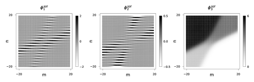
Figure 1: The $(m,n)$-dependence of the components of the two-soliton solution (4.5).

To illustrate the structure of the two-soliton solutions we calculate (4.5) for some fixed set of soliton parameters: $L_{1}=0.1+i$, $L_{2}=0.1+2i$, $a_{1}=10$, $a_{2}=9$. To make the plots more clear we present in figure 1 only the soliton part of the solution, $\boldsymbol{\phi}^{\rm sol}$. As in the one-soliton case, we can see that the third component of $\boldsymbol{\phi}$ (the part of $\boldsymbol{\phi}$ which is parallel to $\boldsymbol{\phi}^{\rm bg}$) has the two-kink structure, while the first two (the part of $\boldsymbol{\phi}$ which is perpendicular to $\boldsymbol{\phi}^{\rm bg}$) have the stucture of two solitons (with sign-alternation along one of the directions).

4.2 Vector Yamilov equation.

To obtain the solitons of equation (1.4) using the result of proposition 3.1 we have to introduce the continuous variable $t$ so that the differentiating $d/dt$ reproduces the action of the operator (2.4) or $\frac{1}{\mu^{2}-\nu^{2}}\left(\mathbb{T}^{\scriptscriptstyle{R}}_{\mu}\left(\mathbb{T}^{\scriptscriptstyle{R}}_{\nu}\right)^{-1}-1\right)$. One can obtain from (3.4) that

$$\left(\mathbb{T}^{\scriptscriptstyle{R}}_{\mu}\left(\mathbb{T}^{\scriptscriptstyle{R}}_{\nu}\right)^{-1}-1\right)\mathsf{A}=2i(\mu-\nu)\;\mathsf{A}\,\mathsf{L}\left(\mathsf{L}-i\mu\right)^{-1}\left(\mathsf{L}+i\nu\right)^{-1}$$ (4.17)

which leads to

$$\frac{d}{dt}\,\mathsf{A}(t)=i\mathsf{A}(t)\;\mathsf{L}\left(\mathsf{L}^{2}+\nu^{2}\right)^{-1}$$ (4.18)

or

$$\mathsf{A}(t)=\mathsf{A}(0)\;\exp\left(i\mathsf{\Omega}t\right),\qquad\mathsf{\Omega}=\mathsf{L}\left(\mathsf{L}^{2}+\nu^{2}\right)^{-1}$$ (4.19)

The $n$-dependence of the matrices $\mathsf{A}$ (and, hence, of $\boldsymbol{\phi}$) is governed, as in the previous section, by the matrix $\mathsf{H}=\mathsf{H}_{\nu}$ from (4.8). Thus, we have all necessary to present the solitons of (1.4).

Proposition 4.2

The $N$-soliton solutions for the vector Yamilov equation (1.4) can be presented as

$$\boldsymbol{\phi}_{n}(t)=\boldsymbol{\phi}^{\rm bg}_{n}(t)+\boldsymbol{\phi}^{\rm sol}_{n}(t)$$ (4.20)

where the background part, $\boldsymbol{\phi}^{\rm bg}_{n}(t)$ is the linear function of $t$ and $n$,

$$\boldsymbol{\phi}^{\rm bg}_{m,n}=\left(\frac{t}{2\nu}+n\nu\right){\scriptstyle\left(\begin{array}[]{c}0\\[-2.84526pt] 0\\[-2.84526pt] 1\end{array}\right)}$$ (4.21)

and

$$\boldsymbol{\phi}^{\rm sol}_{n}(t)=\left(\begin{array}[]{c}\mathop{\mbox{\rm Re}}\langle\beta|\mathsf{G}_{n}(t)\mathsf{A}_{n}(t)|1\rangle\\[5.69054pt] \mathop{\mbox{\rm Im}}\langle\beta|\mathsf{G}_{n}(t)\mathsf{A}_{n}(t)|1\rangle\\[2.84526pt] -\mathop{\mbox{\rm Im}}\langle\beta|\mathsf{G}_{n}(t)|1\rangle\end{array}\right).$$ (4.22)

Here

$$\mathsf{A}_{n}(t)=\mathsf{A}\;\mathsf{H}^{n}\exp\left(i\mathsf{\Omega}t\right),$$ (4.23)

with the constant matrices $\mathsf{A}$, $\mathsf{H}$ and $\mathsf{\Omega}$ given by

$$\mathsf{A}=\left(\;\frac{a_{k}}{\bar{L}_{j}-L_{k}}\;\right)_{j,k=1,...,N}$$ (4.24)

$$\mathsf{H}=\mbox{\rm diag}\left(\;\frac{L_{k}+i\nu}{L_{k}-i\nu}\;\right)_{k=1,...,N},$$ (4.25)

$$\mathsf{\Omega}=\mbox{\rm diag}\left(\;\frac{L_{k}}{L_{k}^{2}+\nu^{2}}\;\right)_{k=1,...,N},$$ (4.26)

and

$$\mathsf{G}_{n}(t)=\left(1+\mathsf{A}_{n}(t)\overline{\mathsf{A}_{n}(t)}\right)^{-1}.$$ (4.27)

The constant $N$-row $\langle\beta|$ is defined by $\langle\beta|=\left(\beta_{1},...,\beta_{N}\right)=\left(a_{1},...,a_{N}\right)\mathsf{A}^{-1}$, the $N$-column $|1\rangle$ is defined as $|1\rangle=\left(1,...,1\right)$ and $\{a_{k},L_{k}\}_{k=1,\dots,N}$ and $\nu$ are arbitrary constants.

Clearly, the structure of the one soliton solution is the same as in the case of the vector discrete KdV equation,

$$\boldsymbol{\phi}^{\rm sol}_{n}(t)=\frac{\rho}{\cosh h_{n}(t)}\left(\cos\varphi_{n}(t),\;\sin\varphi_{n}(t),\;e^{-h_{n}(t)}\right)^{T}.$$ (4.28)

The differences are in that $\rho=|\mathop{\mbox{\rm Im}}L|$ and in the ‘dispersion laws’,

$$h_{n}(t) = -\gamma t+\kappa_{R}(\nu)n+h_{*},$$ (4.29)

$$\varphi_{n}(t) = \omega t+\kappa_{I}(\nu)n+\varphi_{*}$$ (4.30)

where

$$\omega=-\frac{\mathop{\mbox{\rm Im}}a}{2\mathop{\mbox{\rm Im}}L},\qquad\gamma=\frac{\mathop{\mbox{\rm Re}}a}{2\mathop{\mbox{\rm Im}}L}$$ (4.31)

while the functions $\kappa_{R,I}(\nu)$ and the constants $h_{*}$ and $\varphi_{*}$ are defined in (4.14) and (4.15).

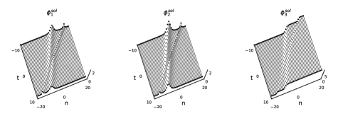
Figure 2: The $(t,n)$-dependence of the components of the two-soliton solution (4.22).

The two-soliton solution for $L_{1}=i$, $L_{2}=2i$, $a_{1}=2+2i$, $a_{2}=2+3i$ and $\nu=-0.8$ is presented in figure 2. Again, the part of $\boldsymbol{\phi}$ which is perpendicular to $\boldsymbol{\phi}^{\rm bg}$ has the structure of two $sech$–solitons, while the part of $\boldsymbol{\phi}$ which is parallel to $\boldsymbol{\phi}^{\rm bg}$ reveals the two–kink behaviour.

5 Discussion.

To conclude, we would like to stress out once more the main difference between the calculations of this work and other our works devoted to solitons of the vector lattice models, for example, [13, 14]. In [13, 14], our starting point was some scalar identitities for the soliton matrices from [11]. These identies were enough to (i) derive the vector ones, similar to equation (2.10), or the first equation from (2.7), and (ii) to tackle the rectrictions similar to the second equation from (2.7). Here, the situation was more complicated: we had to return to the matrices discussed in [11] and to derive some aditional identities (absent in [11]), which are less ‘universal’ but which gave us possibility to construct solitons for the models discussed in this paper.

Finally, according the so-called Hirota’s three-soliton test [15, 16, 17, 18], existence of $N$-soliton solutions can be viewed as an indication of the integrability of the models (1.3) and (1.4). Thus, a natural continuation of this work is to study the corresponding range problems mentioned in the Introduction (the Lax representation, conservation laws, Hamiltonian structures etc). However these questions are out of the scope of this paper and may be considered in the following studies.

References

References

- [1] Capel H W, Wiersma G L and Nijhoff F W 1986 Physica A 138 76–99
- [2] Papageorgiou V G, Nijhoff F W and Capel H W 1990 Phys. Lett. A 147 106–114
- [3] Capel H W, Nijhoff F W and Papageorgiou V G 1991 Phys. Lett. A 155 377–387
- [4] Nijhoff F and Capel H 1995 Acta Appl. Math. 39 133–158
- [5] Adler V E, Bobenko A I and Suris Y B 2003 Commun. Math. Phys. 233 513–543
- [6] Yamilov R I 1983 Uspekhi Mat. Nauk 38 155–156
- [7] Yamilov R 2006 J. Phys. A 39 R541–R623
- [8] Mikhailov A V, Shabat A B and Yamilov R I 1987 Russian Mathematical Surveys 42 1–63
- [9] Pritula G M and Vekslerchik V E 2003 J. Phys. A 36 213–226
- [10] Levi D, Petrera M, Scimiterna C and Yamilov R 2008 SIGMA 4 077
- [11] Vekslerchik V E 2015 J. Phys. A 48 445204
- [12] Miwa T 1982 Proc. Japan Acad. ser.A 58 9–12
- [13] Vekslerchik V 2016 J. Phys. A 49 455202
- [14] Vekslerchik V 2019 SIGMA 15 028
- [15] Hietarinta J 1987 J. Math. Phys. 28 1732–1742
- [16] Hietarinta J 1987 J. Math. Phys. 28 2094–2101
- [17] Hietarinta J 1987 J. Math. Phys. 28 2586–2592
- [18] Ramani A, Grammaticos B and Bountis T 1989 Physics Reports 180 159–245