Arbitrarily High-order Linear Schemes for Gradient Flow Models

Abstract

We present a paradigm for developing arbitrarily high order, linear, unconditionally energy stable numerical algorithms for gradient flow models. We apply the energy quadratization (EQ) technique to reformulate the general gradient flow model into an equivalent gradient flow model with a quadratic free energy and a modified mobility. Given solutions up to $t_{n}=n\Delta t$ with $\Delta t$ the time step size, we linearize the EQ-reformulated gradient flow model in $(t_{n},t_{n+1}]$ by extrapolation. Then we employ an algebraically stable Runge-Kutta method to discretize the linearized model in $(t_{n},t_{n+1}]$. Then we use the Fourier pseudo-spectral method for the spatial discretization to match the order of accuracy in time. The resulting fully discrete scheme is linear, unconditionally energy stable, uniquely solvable, and may reach arbitrarily high order. Furthermore, we present a family of linear schemes based on prediction-correction methods to complement the new linear schemes. Some benchmark numerical examples are given to demonstrate the accuracy and efficiency of the schemes.

Keywords: Energy stable schemes, gradient flow models, Runge-Kutta methods, linear high-order schemes, pseudo-spectral methods.

1 Introduction

For many import phenomena in physics, life science, and engineering, the processes are driven by minimizing the free energy or maximizing entropy, i.e., dissipative dynamics. Gradient flow models are usually used to model these phenomena. The generic form of a gradient flow model is given by

$$\frac{\partial}{\partial t}\Phi=\mathcal{G}\frac{\delta F}{\delta\Phi},$$ (1.1)

with proper boundary conditions. Here $\Phi$ is the thermodynamical variable, $F$ is the free energy for the isothermal system (or entropy for the nonisothermal system), and $\mathcal{G}$ is the mobility operator/matrix. The gradient flow model is thermodynamically consistent if it yields a positive entropy production or negative energy dissipation rate. The classical Allen-Cahn equation [3] and Cahn-Hilliard equation [4] are two examples of gradient flow models (1.1). Other gradient flow models include the molecular beam epitaxy model [8], the phase-field crystal model [10], the thermodynamically consistent dendritic growth model [35], the surfactant model [33], the diblock copolymer model [7] etc.

Most gradient flow models are nonlinear, so that their analytical solutions are intractable. Hence, designing accurate, efficient, and stable algorithms to solve them becomes essential [11, 13, 37, 32, 44, 34, 43]. A numerical scheme that preserves the energy dissipation property is known as an energy stable scheme [11]. It has been shown that schemes that are not energy stable could lead to instability or oscillatory solutions [13]. This is because non-energy-stable schemes may introduce truncation errors that destroy the physical law numerically. Thus, developing energy stable numerical algorithms is necessary for accurately resolving the dynamics of gradient flow models [20, 23, 21, 30, 44].

Over the years, the development of numerical algorithms has been done primarily on a specific gradient flow model, exploiting its specific mathematical properties and structures. The noticeable ones include the Allen-Cahn and Cahn-Hilliard equation [11, 1, 42, 24, 36, 32, 20, 9] as well as the molecular beam epitaxy model [28, 41, 26, 6, 27, 12]. As a result, most numerical algorithms developed for a specific gradient flow model can hardly be applied to another gradient flow model with a different free energy and mobility. The status-quo did not change until the energy quaratization (EQ) approach was introduced a few years ago [39, 44], which turns out to be rather general so that it can be readily applied to general gradient flow models with no restrictions on the specific form of the mobility and free energy [40, 16] (so long as it is bounded below, which is usually the case). Based on the idea of EQ, the scalar auxiliary variable (SAV) approach was introduced later [31], where each time step only linear systems with constant coefficients need to be solved. Several other extensions of EQ and SAV approaches have been explored further. For instance, regularization terms [5] and stabilization terms [38] are added, and the modified energy quadratization technique [25, 22] are introduced to improve the EQ methodology. We notice that most existing schemes related to the EQ methodology are up to 2nd order accurate in time. Some higher-order ETD schemes have been introduced to solve the MBE model and Cahn-Hilliard models recently, but their theoretical proofs of energy stability are still missing. Shen et al. [30] remarked on higher-order BDF schemes using the SAV approach, but no rigorous theoretical proofs are available.

Recently, Gong et al. [19, 18, 15] introduced the arbitrarily high-order schemes for solving gradient flow models by combining the methodology of energy quadratization with quadratic invariant Runge-Kutta (RK) methods. This seminal idea sheds light on solving gradient flow models with an arbitrarily high order of accuracy. We note that the proposed high order schemes are fully nonlinear so that the solution existence and uniqueness are not guaranteed when the time step is large. Moreover, the implementation can be complicated compared to linear schemes. Often, it requires iterations at each time step, which adds up to the computational cost.

In this paper, we will address these issues by proposing a new paradigm for developing arbitrarily high order schemes that are unconditionally energy stable and linear. As a significant advance over our previous work, the newly proposed paradigm would result in linear schemes, while preserving unconditional energy stability. These newly proposed schemes will bring in significant improvement in numerical implementation and reduction in computational cost. First of all, as the schemes are all linear, only linear systems need to be solved at each time step. Therefore, they are easy to implement and computationally efficient. In addition, the existence and uniqueness of the numerical solutions can be guaranteed, which is actually independent of the time steps. In other words, larger time steps can be readily applied so long as the accuracy requirement is met. This is warranted by the existence of a unique solution and unconditionally energy stable. Equipped with the benefits of EQ method and RK method, the newly proposed schemes apply to general gradient flow models. For illustration purposes, we solve the Cahn-Hilliard model and the molecular beam epitaxy model to demonstrate the effectiveness of some selected new schemes. To show their accuracy and efficiency, we also compare two proposed schemes with the $2$nd order convex splitting schemes.

The rest of this paper is organized as follows. In Section 2, we briefly introduce the general gradient flow model and use the EQ method to reformulate it into an equivalent form. In Section 3, the arbitrarily high-order linear energy stable schemes are introduced, and their energy stability and uniquely solvability are discussed. In Section 4, several numerical examples are shown to illustrate the power of our proposed arbitrarily high order schemes. In the end, some concluding remarks are given.

2 Gradient Flow Models and Their EQ Reformulation

In this section, we present the general gradient flow model firstly and then apply the energy quadratization technique to reformulate the model into an equivalent gradient flow form with a quadratic energy functional, a modified mobility matrix and the corresponding energy dissipation law, which is called the EQ reformulated model. The EQ reformulation for this class of gradient flow models provides an elegant platform for developing arbitrarily high-order unconditionally energy stable schemes [19, 15].

2.1 Gradient flow models

Mathematically, the form of a general gradient flow model is given by [44, 31]

$$\frac{\partial}{\partial t}\Phi=\mathcal{G}\frac{\delta F}{\delta\Phi},$$ (2.1)

where $\Phi=(\phi_{1},\cdots,\phi_{d})^{T}$ is the state variable vector, $\mathcal{G}$ is the $d\times d$ mobility matrix operator which can depend on $\Phi$, $F$ is the free energy, and $\frac{\delta F}{\delta\Phi}$ is the variational derivative of the free energy functional with respect to the state variable, known as the chemical potential. The triple $(\Phi,\mathcal{G},F)$ uniquely defines the gradient flow model. For (2.1) to be thermodynamically consistent, the time rate of change of the free energy must be non-increasing:

$$\frac{dF}{dt}=\left(\frac{\delta F}{\delta\Phi},\frac{\partial\Phi}{\partial t}\right)=\left(\frac{\delta F}{\delta\Phi},\mathcal{G}\frac{\delta F}{\delta\Phi}\right)\leq 0,$$ (2.2)

where the inner product is defined by $({\bf f},{\bf g})=\sum\limits_{i=1}^{d}\int_{\Omega}f_{i}g_{i}d\mathbf{x}$, $\forall\mathbf{f},\mathbf{g}\in\big{(}L^{2}(\Omega)\big{)}^{d}$, which requires $\mathcal{G}$ to be negative semi-definite. The $L^{2}$ norm is defined as $\|\bf f\|_{2}=\sqrt{({\bf f},{\bf g})}$. Note that the energy dissipation law (2.2) holds only for suitable boundary conditions. Such boundary conditions include periodic boundary conditions and the other boundary conditions that make the boundary integrals resulted from the integration by parts vanish in the calculation of variational derivatives. In this paper, we limit our study to these boundary conditions.

2.2 Model reformulation using the EQ approach

We reformulate the gradient flow model (2.1) by transforming the free energy into a quadratic form using nonlinear transformations. For the purpose of illustration, we assume the free energy is given by the following

$$F=\frac{1}{2}(\Phi,\mathcal{L}\Phi)+\big{(}f(\Phi,\nabla\Phi),1\big{)},$$ (2.3)

where $\mathcal{L}$ is a linear, self-adjoint, positive semi-definite operator (independent of $\Phi$), and $f$ is the bulk part of the free energy density, which has a lower bound. Then the free energy $F$ can be rewritten into a quadratic form

$$\mathcal{F}=\frac{1}{2}(\Phi,\mathcal{L}\Phi)+\|q\|^{2}-C|\Omega|,$$ (2.4)

by introducing an auxiliary variable $q=\sqrt{f(\Phi,\nabla\Phi)+C}$, where $C$ is a positive constant large enough to make $q$ real-valued for all $\Phi$.

We denote $g[\Phi]=\sqrt{f(\Phi,\nabla\Phi)+C}$. Then model (2.1) can be reformulated into the following equivalent system

$$\left\{\begin{array}[]{l}\Phi_{t}=\mathcal{G}\bigg{(}\mathcal{L}\Phi+2q\frac{\partial g}{\partial\Phi}-\nabla\cdot\Big{(}2q\frac{\partial g}{\partial\nabla\Phi}\Big{)}\bigg{)},\\ q_{t}=\frac{\partial g}{\partial\Phi}\cdot\Phi_{t}+\frac{\partial g}{\partial\nabla\Phi}\cdot\nabla\Phi_{t},\end{array}\right.$$ (2.5)

with initial conditions

$$\Phi(\mathbf{x},0)=\Phi_{0}(\mathbf{x}),\quad q(\mathbf{x},0)=\sqrt{f\big{(}\Phi_{0}(\mathbf{x}),\nabla\Phi_{0}(\mathbf{x})\big{)}+C}.$$ (2.6)

It is readily to prove that the reformulated system (2.5) preserves the following energy dissipation law

$$\frac{d\mathcal{F}}{dt}=\Bigg{(}\mathcal{L}\Phi+2q\frac{\partial g}{\partial\Phi}-\nabla\cdot\Big{(}2q\frac{\partial g}{\partial\nabla\Phi}\Big{)},\mathcal{G}\bigg{(}\mathcal{L}\Phi+2q\frac{\partial g}{\partial\Phi}-\nabla\cdot\Big{(}2q\frac{\partial g}{\partial\nabla\Phi}\Big{)}\bigg{)}\Bigg{)}\leq 0.$$ (2.7)

We introduce

$$\mathbf{u}=(\Phi,q)^{T}$$ (2.8)

and recast system (2.5) into a compact gradient flow form

$$\mathbf{u}_{t}=\mathcal{M}\frac{\delta\mathcal{F}}{\delta\mathbf{u}},$$ (2.9)

with a modified mobility operator

$$\mathcal{M}=\left(\begin{array}[]{c}1\\ \frac{\partial g}{\partial\Phi}+\frac{\partial g}{\partial\nabla\Phi}\cdot\nabla\end{array}\right)\mathcal{G}\left(1,\frac{\partial g}{\partial\Phi}-\nabla\cdot\frac{\partial g}{\partial\nabla\Phi}\right).$$ (2.10)

The energy dissipation law given in (2.7) is recast into

$$\frac{d\mathcal{F}}{dt}=\Big{(}\frac{\delta\mathcal{F}}{\delta\mathbf{u}},\mathcal{M}\frac{\delta\mathcal{F}}{\delta\mathbf{u}}\Big{)}\leq 0.$$ (2.11)

Since the EQ-reformulated form in (2.5) has a quadratic free energy, we next discuss how to devise linear high-order energy stable schemes for it.

3 High-order linear energy stable schemes

In this section, we first derive a high-precision linear gradient-flow system to approximate EQ-reformulated model (2.5) up to $t_{n}=n\Delta t$, where $\Delta t$ is the time step. In particular, the corresponding energy dissipation law is inherited. Then the algebraically stable RK method [2] is applied to the resulting linear gradient-flow system to develop a class of linear semi-discrete schemes in time. We name the schemes linear energy quadratizatized Runge-Kutta (LEQRK) methods. In order to improve accuracy and stability, a prediction-correction technique is proposed for the LEQRK schemes, leading to the LEQRK-PC methods. These new algorithms are linear, unconditionally energy stable, and can be devised at any desired order in time.

3.1 LEQRK schemes

Assuming numerical solutions of $\Phi$ up to $t\leq t_{n}$ have been obtained, we then solve system (2.5) in $t\in(t_{n},t_{n+1}]$ approximately. We utilize the numerical solutions of $\Phi$ at $t\leq t_{n}$ to obtain its interpolating polynomial approximation denoted by $\Phi_{N}(t)$. Then we approximate model (2.5) in $(t_{n},t_{n+1}]$ using the following linear, variable coefficient gradient flow system

$$\left\{\begin{array}[]{l}\Phi_{t}=\mathcal{G}\bigg{(}\mathcal{L}\Phi+2q\frac{\partial g_{N}}{\partial\Phi}-\nabla\cdot\Big{(}2q\frac{\partial g_{N}}{\partial\nabla\Phi}\Big{)}\bigg{)},\\ q_{t}=\frac{\partial g_{N}}{\partial\Phi}\cdot\Phi_{t}+\frac{\partial g_{N}}{\partial\nabla\Phi}\cdot\nabla\Phi_{t},\end{array}\right.$$ (3.1)

where $\frac{\partial g_{N}}{\partial\Phi}=\frac{\partial g}{\partial\Phi}[\Phi_{N}(t)]$ and $\frac{\partial g_{N}}{\partial\nabla\Phi}=\frac{\partial g}{\partial\nabla\Phi}[\Phi_{N}(t)]$ are independent of $\Phi$. The linear gradient flow system (3.1) satisfies the following energy dissipation law

$$\frac{d\mathcal{F}}{dt}=\Bigg{(}\mathcal{L}\Phi+2q\frac{\partial g_{N}}{\partial\Phi}-\nabla\cdot\Big{(}2q\frac{\partial g_{N}}{\partial\nabla\Phi}\Big{)},\mathcal{G}\bigg{(}\mathcal{L}\Phi+2q\frac{\partial g_{N}}{\partial\Phi}-\nabla\cdot\Big{(}2q\frac{\partial g_{N}}{\partial\nabla\Phi}\Big{)}\bigg{)}\Bigg{)}\leq 0.$$ (3.2)

Applying a $s$-stage RK method for the linear system (3.1), we obtain the following LEQRK scheme.

Scheme 3.1 ($s$-stage LEQRK Scheme).

Let $b_{i}$, $a_{ij}$ ($i,j=1,\cdots,s$) be real numbers and let $c_{i}=\sum\limits_{j=1}^{s}a_{ij}$. For given $(\Phi^{n},q^{n})$ and $\Phi_{N}(t_{n}+c_{i}\Delta t),\forall i$, the following intermediate values are first calculated by

$$\left\{\begin{array}[]{l}\Phi_{i}^{n}=\Phi^{n}+\Delta t\sum\limits_{j=1}^{s}a_{ij}k_{j}^{n},\\ Q_{i}^{n}=q^{n}+\Delta t\sum\limits_{j=1}^{s}a_{ij}l_{j}^{n},\\ k_{i}^{n}=\mathcal{G}\bigg{(}\mathcal{L}\Phi_{i}^{n}+2Q_{i}^{n}\Big{(}\frac{\partial g}{\partial\Phi}\Big{)}_{i}^{n,*}-\nabla\cdot\Big{(}2Q_{i}^{n}\Big{(}\frac{\partial g}{\partial\nabla\Phi}\Big{)}_{i}^{n,*}\Big{)}\bigg{)},\\ l_{i}^{n}=\Big{(}\frac{\partial g}{\partial\Phi}\Big{)}_{i}^{n,*}\cdot k_{i}^{n}+\Big{(}\frac{\partial g}{\partial\nabla\Phi}\Big{)}_{i}^{n,*}\cdot\nabla k_{i}^{n},\end{array}\right.\quad i=1,\cdots,s,$$ (3.3)

where $\Big{(}\frac{\partial g}{\partial\Phi}\Big{)}_{i}^{n,*}=\frac{\partial g}{\partial\Phi}[\Phi_{N}(t_{n}+c_{i}\Delta t)]$ and $\Big{(}\frac{\partial g}{\partial\nabla\Phi}\Big{)}_{i}^{n,*}=\frac{\partial g}{\partial\nabla\Phi}[\Phi_{N}(t_{n}+c_{i}\Delta t)]$. Then $(\Phi^{n+1},q^{n+1})$ is updated via

$$\Phi^{n+1}=\Phi^{n}+\Delta t\sum\limits_{i=1}^{s}b_{i}k_{i}^{n},$$ (3.4)

$$q^{n+1}=q^{n}+\Delta t\sum\limits_{i=1}^{s}b_{i}l_{i}^{n}.$$ (3.5)

Definition 3.1 (Algebraically Stable RK Method [2]).

Denote a symmetric matrix $\mathbf{M}$ with the elements $\mathbf{M}_{ij}=b_{i}a_{ij}+b_{j}a_{ji}-b_{i}b_{j}.$ A RK method is said to be algebraically stable if its RK coefficients satisfy stability condition

$$b_{i}\geq 0,~{}\forall i=1,2,\cdots,s,\quad\textrm{and~{}}\mathbf{M}\textrm{~{}is~{}positive~{}semi-definite}.$$ (3.6)

Next, we show that the algebraically stable LEQRK scheme is unconditionally energy stable.

Theorem 3.1.

The LEQRK scheme with their RK coefficients satisfying stability condition (3.6) is unconditionally energy stable, i.e., it satisfies

$$\mathcal{F}^{n+1}\leq\mathcal{F}^{n},$$ (3.7)

where $\mathcal{F}^{n}=\frac{1}{2}(\Phi^{n},\mathcal{L}\Phi^{n})+\|q^{n}\|^{2}-C|\Omega|.$

Proof.

Denoting $\Phi^{n+1}=\Phi^{n}+\Delta t\sum\limits_{i=1}^{s}b_{i}k_{i}^{n}$ and noticing that operator $\mathcal{L}$ is linear and self-adjoint, we have

$$\frac{1}{2}(\Phi^{n+1},\mathcal{L}\Phi^{n+1})-\frac{1}{2}(\Phi^{n},\mathcal{L}\Phi^{n})=\Delta t\sum\limits_{i=1}^{s}b_{i}(k_{i}^{n},\mathcal{L}\Phi^{n})+\frac{\Delta t^{2}}{2}\sum\limits_{i,j=1}^{s}b_{i}b_{j}(k_{i}^{n},\mathcal{L}k_{j}^{n}).$$ (3.8)

Applying $\Phi^{n}=\Phi_{i}^{n}-\Delta t\sum\limits_{j=1}^{s}a_{ij}k_{j}^{n}$ to the right of (3.8), we deduce

$$\frac{1}{2}(\Phi^{n+1},\mathcal{L}\Phi^{n+1})-\frac{1}{2}(\Phi^{n},\mathcal{L}\Phi^{n})=\Delta t\sum\limits_{i=1}^{s}b_{i}(k_{i}^{n},\mathcal{L}\Phi_{i}^{n})-\frac{\Delta t^{2}}{2}\sum\limits_{i,j=1}^{s}\mathbf{M}_{ij}(k_{i}^{n},\mathcal{L}k_{j}^{n}),$$ (3.9)

where $\sum\limits_{i,j=1}^{s}b_{i}a_{ij}(k_{i}^{n},\mathcal{L}k_{j}^{n})=\sum\limits_{i,j=1}^{s}b_{j}a_{ji}(k_{i}^{n},\mathcal{L}k_{j}^{n})$ and $\mathbf{M}_{ij}=b_{i}a_{ij}+b_{j}a_{ji}-b_{i}b_{j}$ are used. Note that $\mathcal{L}$ can be denoted as $\mathcal{L}=\mathcal{A}^{*}\mathcal{A},$ where $\mathcal{A}$ is a linear operator and $\mathcal{A}^{*}$ is the adjoint operator of $\mathcal{A}$. Since $\mathbf{M}$ is positive semi-definite, we have

$$\sum\limits_{i,j=1}^{s}\mathbf{M}_{ij}(k_{i}^{n},\mathcal{L}k_{j}^{n})=\sum\limits_{i,j=1}^{s}\mathbf{M}_{ij}(\mathcal{A}k_{i}^{n},\mathcal{A}k_{j}^{n})\geq 0.$$ (3.10)

Combining eqs. (3.9) and (3.10) leads to

$$\frac{1}{2}(\Phi^{n+1},\mathcal{L}\Phi^{n+1})-\frac{1}{2}(\Phi^{n},\mathcal{L}\Phi^{n})\leq\Delta t\sum\limits_{i=1}^{s}b_{i}(k_{i}^{n},\mathcal{L}\Phi_{i}^{n}).$$ (3.11)

Similarly, we have

$$\|q^{n+1}\|^{2}-\|q^{n}\|^{2}\leq 2\Delta t\sum\limits_{i=1}^{s}b_{i}(l_{i}^{n},Q_{i}^{n}).$$ (3.12)

Adding (3.11) and (3.12) and noticing that $l_{i}^{n}=\Big{(}\frac{\partial g}{\partial\Phi}\Big{)}_{i}^{n,*}\cdot k_{i}^{n}+\Big{(}\frac{\partial g}{\partial\nabla\Phi}\Big{)}_{i}^{n,*}\cdot\nabla k_{i}^{n}$, we obtain

$$\mathcal{F}^{n+1}-\mathcal{F}^{n}\leq\Delta t\sum\limits_{i=1}^{s}b_{i}\bigg{(}\mathcal{L}\Phi_{i}^{n}+2Q_{i}^{n}\Big{(}\frac{\partial g}{\partial\Phi}\Big{)}_{i}^{n,*}-\nabla\cdot\Big{(}2Q_{i}^{n}\Big{(}\frac{\partial g}{\partial\nabla\Phi}\Big{)}_{i}^{n,*}\Big{)},k_{i}^{n}\bigg{)}.$$ (3.13)

Substituting $k_{i}^{n}=\mathcal{G}\bigg{(}\mathcal{L}\Phi_{i}^{n}+2Q_{i}^{n}\Big{(}\frac{\partial g}{\partial\Phi}\Big{)}_{i}^{n,*}-\nabla\cdot\Big{(}2Q_{i}^{n}\Big{(}\frac{\partial g}{\partial\nabla\Phi}\Big{)}_{i}^{n,*}\Big{)}\bigg{)}$ in (3.13) and noticing the negative semi-definite property of $\mathcal{G}$ and $b_{i}\geq 0,\forall i$, we arrive at $\mathcal{F}^{n+1}-\mathcal{F}^{n}\leq 0.$ This completes the proof. ∎

Remark 3.1.

Note that the Gauss method is a special kind of algebraically stable RK method, whose RK coefficients satisfy $\mathbf{M}={\bf 0}$. Thus the Gauss method preserves the discrete energy dissipation law

$$\mathcal{F}^{n+1}-\mathcal{F}^{n}=\Delta t\sum\limits_{i=1}^{s}b_{i}\bigg{(}\mathcal{L}\Phi_{i}^{n}+2Q_{i}^{n}\Big{(}\frac{\partial g}{\partial\Phi}\Big{)}_{i}^{n,*}-\nabla\cdot\Big{(}2Q_{i}^{n}\Big{(}\frac{\partial g}{\partial\nabla\Phi}\Big{)}_{i}^{n,*}\Big{)},k_{i}^{n}\bigg{)}\leq 0.$$ (3.14)

Remark 3.2.

After appropriate spatial discretization that satisfies the discrete integration-by-parts formula (see [16, 17] for details), the algebraically stable LEQRK scheme naturally leads to a fully discrete energy stable scheme. In this paper, we employ the Fourier pseudo-spectral method for spatial discretization. We omit the details here due to space limitation. Interested readers are referred to our ealier work [16, 19] for details.

Next, we discuss the solvability of the resulting fully discrete scheme.

Theorem 3.2.

If RK coefficient matrix $\mathbf{A}=(a_{ij})$ is positive semi-definite and mobility operator $\mathcal{G}$ satisfies $\mathcal{G}=-\mathcal{B}^{*}\mathcal{B}$, the fully discrete scheme derived by applying the Fourier pseudo-spectral method to Scheme 3.1 is uniquely solvable.

Proof.

Without loss of generality, we still use the notations $\mathcal{G}$, $\mathcal{L}$ and $\nabla$ to denote the corresponding discrete operators in the fully discrete scheme. We consider the homogeneous linear equation system of (3.3)

$$\left\{\begin{array}[]{l}\Phi_{i}^{n}=\Delta t\sum\limits_{j=1}^{s}a_{ij}k_{j}^{n},\\ Q_{i}^{n}=\Delta t\sum\limits_{j=1}^{s}a_{ij}l_{j}^{n},\\ k_{i}^{n}=\mathcal{G}\bigg{(}\mathcal{L}\Phi_{i}^{n}+2Q_{i}^{n}\Big{(}\frac{\partial g}{\partial\Phi}\Big{)}_{i}^{n,*}-\nabla\cdot\Big{(}2Q_{i}^{n}\Big{(}\frac{\partial g}{\partial\nabla\Phi}\Big{)}_{i}^{n,*}\Big{)}\bigg{)},\\ l_{i}^{n}=\Big{(}\frac{\partial g}{\partial\Phi}\Big{)}_{i}^{n,*}\cdot k_{i}^{n}+\Big{(}\frac{\partial g}{\partial\nabla\Phi}\Big{)}_{i}^{n,*}\cdot\nabla k_{i}^{n},\end{array}\right.\quad i=1,\cdots,s,$$ (3.15)

where $\Phi_{i}^{n},Q_{i}^{n},k_{i}^{n},l_{i}^{n}$ are unknown. To prove unique solvability of the fully discrete scheme, we need to prove that the homogeneous linear equation system (3.15) admits only a zero solution.

Computing the discrete inner product of the third equation in (3.15) with $\mathcal{L}\Phi_{i}^{n}+2Q_{i}^{n}\Big{(}\frac{\partial g}{\partial\Phi}\Big{)}_{i}^{n,*}-\nabla\cdot\Big{(}2Q_{i}^{n}\Big{(}\frac{\partial g}{\partial\nabla\Phi}\Big{)}_{i}^{n,*}\Big{)}$ and sum over $i$, we deduce from (3.15)

$$\Delta t\sum\limits_{i,j=1}^{s}a_{ij}(\mathcal{A}k_{i}^{n},\mathcal{A}k_{j}^{n})+2\Delta t\sum\limits_{i,j=1}^{s}a_{ij}(l_{i}^{n},l_{j}^{n})+\sum\limits_{i=1}^{s}\Bigg{\|}\mathcal{B}\bigg{(}\mathcal{L}\Phi_{i}^{n}+2Q_{i}^{n}\Big{(}\frac{\partial g}{\partial\Phi}\Big{)}_{i}^{n,*}-\nabla\cdot\Big{(}2Q_{i}^{n}\Big{(}\frac{\partial g}{\partial\nabla\Phi}\Big{)}_{i}^{n,*}\Big{)}\bigg{)}\Bigg{\|}^{2}=0,$$

where $\mathcal{G}=-\mathcal{B}^{*}\mathcal{B}$ and $\mathcal{L}=\mathcal{A}^{*}\mathcal{A}$ are used. Since $\mathbf{A}=(a_{ij})$ is positive semi-definite, which implies that the first two terms of the above equation are nonnegative, thus we have

$$\mathcal{B}\bigg{(}\mathcal{L}\Phi_{i}^{n}+2Q_{i}^{n}\Big{(}\frac{\partial g}{\partial\Phi}\Big{)}_{i}^{n,*}-\nabla\cdot\Big{(}2Q_{i}^{n}\Big{(}\frac{\partial g}{\partial\nabla\Phi}\Big{)}_{i}^{n,*}\Big{)}\bigg{)}=0,\quad\forall i,$$ (3.16)

which leads to

$$\mathcal{G}\bigg{(}\mathcal{L}\Phi_{i}^{n}+2Q_{i}^{n}\Big{(}\frac{\partial g}{\partial\Phi}\Big{)}_{i}^{n,*}-\nabla\cdot\Big{(}2Q_{i}^{n}\Big{(}\frac{\partial g}{\partial\nabla\Phi}\Big{)}_{i}^{n,*}\Big{)}\bigg{)}=0,\quad\forall i.$$ (3.17)

Therefore, according to (3.15), we arrive at

$$k_{i}^{n}=0,\quad l_{i}^{n}=0,\quad\Phi_{i}^{n}=0,\quad Q_{i}^{n}=0,\quad\forall i.$$ (3.18)

This completes the proof. ∎

Theorem 3.3.

If diagnally implicit RK coefficients satisfy $a_{ii}>0$, then the fully discrete scheme derived by applying the Fourier pseudo-spectral method to Scheme 3.1 is uniquely solvable.

Proof.

For the diagnally implicit RK (DIRK) scheme, we solve $\Phi_{i}^{n},Q_{i}^{n},k_{i}^{n},l_{i}^{n}$ in turn from $i=1$ to $s$. Therefore, we here consider the following homogeneous linear equation system

$$\left\{\begin{array}[]{l}\Phi_{i}^{n}=\Delta ta_{ii}k_{i}^{n},\\ Q_{i}^{n}=\Delta ta_{ii}l_{i}^{n},\\ k_{i}^{n}=\mathcal{G}\bigg{(}\mathcal{L}\Phi_{i}^{n}+2Q_{i}^{n}\Big{(}\frac{\partial g}{\partial\Phi}\Big{)}_{i}^{n,*}-\nabla\cdot\Big{(}2Q_{i}^{n}\Big{(}\frac{\partial g}{\partial\nabla\Phi}\Big{)}_{i}^{n,*}\Big{)}\bigg{)},\\ l_{i}^{n}=\Big{(}\frac{\partial g}{\partial\Phi}\Big{)}_{i}^{n,*}\cdot k_{i}^{n}+\Big{(}\frac{\partial g}{\partial\nabla\Phi}\Big{)}_{i}^{n,*}\cdot\nabla k_{i}^{n},\end{array}\right.$$ (3.19)

where $\Phi_{i}^{n},Q_{i}^{n},k_{i}^{n},l_{i}^{n}$ are unknown. To prove unique solvability of the fully discrete scheme, we need to prove that homogeneous linear equation system (3.19) admits only a zero solution.

Similar to the proof of Theorem 3.2, we have

$$\Delta ta_{ii}\|\mathcal{A}k_{i}^{n}\|^{2}+2\Delta ta_{ii}\|l_{i}^{n}\|^{2}$$

$$= \Bigg{(}\mathcal{L}\Phi_{i}^{n}+2Q_{i}^{n}\Big{(}\frac{\partial g}{\partial\Phi}\Big{)}_{i}^{n,*}-\nabla\cdot\Big{(}2Q_{i}^{n}\Big{(}\frac{\partial g}{\partial\nabla\Phi}\Big{)}_{i}^{n,*}\Big{)},\mathcal{G}\bigg{(}\mathcal{L}\Phi_{i}^{n}+2Q_{i}^{n}\Big{(}\frac{\partial g}{\partial\Phi}\Big{)}_{i}^{n,*}-\nabla\cdot\Big{(}2Q_{i}^{n}\Big{(}\frac{\partial g}{\partial\nabla\Phi}\Big{)}_{i}^{n,*}\Big{)}\bigg{)}\Bigg{)}$$

$$\leq 0,$$

which leads to

$$\mathcal{A}k_{i}^{n}=0,\quad l_{i}^{n}=0.$$ (3.20)

Combining (3.19) and (3.20), we deduce in turn

$$l_{i}^{n}=0,\quad Q_{i}^{n}=0,\quad\mathcal{L}k_{i}^{n}=0,\quad\mathcal{L}\Phi_{i}^{n}=0,\quad k_{i}^{n}=0,\quad\Phi_{i}^{n}=0.$$ (3.21)

This completes the proof. ∎

Remark 3.3.

In this paper, we give examples in two 4th-order algebraically stable RK methods, i.e., Gauss4th and DIRK4th given by the Butcher tables, respectively,

$$\begin{array}[]{c|cc}\frac{1}{2}-\frac{\sqrt{3}}{6}&\frac{1}{4}&\frac{1}{4}-\frac{\sqrt{3}}{6}\\ \frac{1}{2}+\frac{\sqrt{3}}{6}&\frac{1}{4}+\frac{\sqrt{3}}{6}&\frac{1}{4}\\ \hline\cr&\frac{1}{2}&\frac{1}{2}\\ \end{array},\qquad\qquad\begin{array}[]{c|ccc}\sigma&\sigma&0&0\\ \frac{1}{2}&\frac{1}{2}-\sigma&\sigma&0\\ 1-\sigma&2\sigma&1-4\sigma&\sigma\\ \hline\cr&\mu&1-2\mu&\mu\\ \end{array},$$

with $\sigma=\cos(\pi/18)/\sqrt{3}+1/2$, $\mu=1/\big{(}6(2\sigma-1)^{2}\big{)}$. We note that Gauss4th and DIRK4th satisfy the conditions in Theorem 3.2 and Theorem 3.3, respectively. Therefore, after an appropriate spatial discretization, the LEQRK schemes equipped with Gauss4th or DIRK4th are uniquely solvable.

Remark 3.4.

Noticing that $\Phi_{i}^{m}$ approximates $\Phi(t_{m}+c_{i}\Delta t)$, we can choose the time nodes $t_{m}$, $t_{m}+c_{i}\Delta t$ ($m<n$) and $t_{n}$ as the interpolation points to obtain the interpolation polynomial $\Phi_{N}(t)$. However, too many interpolation points will cause the interpolation polynomial to be highly oscillating, which may make $\Phi_{N}(t_{n}+c_{i}\Delta t)$ an inaccurate extrapolation for $\Phi(t_{n}+c_{i}\Delta t)$. Therefore, we only take $t_{n-1}$, $t_{n-1}+c_{i}\Delta t,~{}\forall i$ and $t_{n}$ as the interpolation points in this paper. For example, for the Gauss4th method, we choose the interpolation points $(t_{n-1},\Phi^{n-1})$, $(t_{n-1}+c_{1}\Delta t,\Phi_{1}^{n-1})$, $(t_{n-1}+c_{2}\Delta t,\Phi_{2}^{n-1})$, $(t_{n},\Phi^{n})$ and obtain the corresponding interpolation polynomial

$$\Phi_{N}(t_{n-1}+s\Delta t) = \frac{(s-c_{1})(s-c_{2})(s-1)}{-c_{1}c_{2}}\Phi^{n-1}+\frac{s(s-c_{2})(s-1)}{c_{1}(c_{1}-c_{2})(c_{1}-1)}\Phi_{1}^{n-1}$$

$$+\frac{s(s-c_{1})(s-1)}{c_{2}(c_{2}-c_{1})(c_{2}-1)}\Phi_{2}^{n-1}+\frac{s(s-c_{1})(s-c_{2})}{(1-c_{1})(1-c_{2})}\Phi^{n},$$

where $c_{1}=1/2-\sqrt{3}/6$ and $c_{2}=1/2+\sqrt{3}/6$. Thus we have

$$\Phi_{N}(t_{n}+c_{1}\Delta t)=(2\sqrt{3}-4)\Phi^{n-1}+(7\sqrt{3}-11)\Phi_{1}^{n-1}+(6-5\sqrt{3})\Phi_{2}^{n-1}+(10-4\sqrt{3})\Phi^{n},$$ (3.22)

$$\Phi_{N}(t_{n}+c_{2}\Delta t)=-(2\sqrt{3}+4)\Phi^{n-1}+(6+5\sqrt{3})\Phi_{1}^{n-1}-(7\sqrt{3}+11)\Phi_{2}^{n-1}+(10+4\sqrt{3})\Phi^{n}.$$ (3.23)

Replacing $n$ with $n-1$ in the first equation of (3.3) and (3.4), then we deduce

$$\Phi^{n}=\Phi^{n-1}-\sqrt{3}\Phi_{1}^{n-1}+\sqrt{3}\Phi_{2}^{n-1}.$$ (3.24)

According to (3.22)-(3.24), we obtain

$$\Phi_{N}(t_{n}+c_{1}\Delta t)=(6-2\sqrt{3})\Phi^{n-1}+(1-3\sqrt{3})\Phi_{1}^{n-1}+(5\sqrt{3}-6)\Phi_{2}^{n-1},$$ (3.25)

$$\Phi_{N}(t_{n}+c_{2}\Delta t)=(6+2\sqrt{3})\Phi^{n-1}-(5\sqrt{3}+6)\Phi_{1}^{n-1}+(1+3\sqrt{3})\Phi_{2}^{n-1}.$$ (3.26)

Note that if we take $t_{n-1}$, $t_{n-1}+c_{i}\Delta t~{}(i=1,2)$ as the interpolation points, we can also derive (3.25)-(3.26), which implies that the LEQRK scheme induced by the Gauss4th method and the interpolations (3.22)-(3.23) or (3.25)-(3.26) may achieve third order accuracy.

3.2 LEQRK-PC schemes

To improve the accuracy as well as stability of Scheme 3.1, we propose a prediction-correction scheme motivated by the works in [14, 29, 19]. Employing the prediction-correction strategy to Scheme 3.1, we obtain the following prediction-correction method:

Scheme 3.2 ($s$-stage LEQRK-PC Scheme).

Let $b_{i}$, $a_{ij}$ ($i,j=1,\cdots,s$) be real numbers and let $c_{i}=\sum\limits_{j=1}^{s}a_{ij}$. For given $(\Phi^{n},q^{n})$ and $\Phi_{N}(t_{n}+c_{i}\Delta t),Q_{N}(t_{n}+c_{i}\Delta t),\forall i$, the following intermediate values are first calculated by the following prediction-correction strategy

1. Prediction: we set $\Phi_{i}^{n,0}=\Phi_{N}(t_{n}+c_{i}\Delta t),$ $Q_{i}^{n,0}=Q_{N}(t_{n}+c_{i}\Delta t)$. Let $M>0$ be a given integer. For $m=0$ to $M-1$, we compute $\Phi_{i}^{n,m+1}$, $k_{i}^{n,m+1}$, $l_{i}^{n,m+1}$, $Q_{i}^{n,m+1}$ using

   $$\left\{\begin{array}[]{l}\Phi_{i}^{n,m+1}=\Phi^{n}+\Delta t\sum\limits_{j=1}^{s}a_{ij}k_{j}^{n,m+1},\\ k_{i}^{n,m+1}=\mathcal{G}\bigg{(}\mathcal{L}\Phi_{i}^{n,m+1}+2Q_{i}^{n,m}\frac{\partial g}{\partial\Phi}[\Phi_{i}^{n,m}]-\nabla\cdot\Big{(}2Q_{i}^{n,m}\frac{\partial g}{\partial\nabla\Phi}[\Phi_{i}^{n,m}]\Big{)}\bigg{)},\\ l_{i}^{n,m+1}=\frac{\partial g}{\partial\Phi}[\Phi_{i}^{n,m+1}]\cdot k_{i}^{n,m+1}+\frac{\partial g}{\partial\nabla\Phi}[\Phi_{i}^{n,m+1}]\cdot\nabla k_{i}^{n,m+1},\\ Q_{i}^{n,m+1}=q^{n}+\Delta t\sum\limits_{j=1}^{s}a_{ij}l_{j}^{n,m+1},\end{array}\right.\quad i=1,\cdots,s.$$ (3.27)

   If $\max\limits_{i}\|\Phi^{n,m+1}_{i}-\Phi^{n,m}_{i}\|_{\infty}<TOL$, we stop the iteration and set $\Phi^{n,*}_{i}=\Phi_{i}^{n,m+1}$; otherwise, we set $\Phi^{n,*}_{i}=\Phi_{i}^{n,M}$.

2. Correction: for the predicted $\Phi^{n,*}_{i}$, we compute the intermediate values $\Phi_{i}^{n},Q_{i}^{n},k_{i}^{n},l_{i}^{n}$ via

   $$\left\{\begin{array}[]{l}\Phi_{i}^{n}=\Phi^{n}+\Delta t\sum\limits_{j=1}^{s}a_{ij}k_{j}^{n},\\ Q_{i}^{n}=q^{n}+\Delta t\sum\limits_{j=1}^{s}a_{ij}l_{j}^{n},\\ k_{i}^{n}=\mathcal{G}\bigg{(}\mathcal{L}\Phi_{i}^{n}+2Q_{i}^{n}\frac{\partial g}{\partial\Phi}[\Phi_{i}^{n,*}]-\nabla\cdot\Big{(}2Q_{i}^{n}\frac{\partial g}{\partial\nabla\Phi}[\Phi_{i}^{n,*}]\Big{)}\bigg{)},\\ l_{i}^{n}=\frac{\partial g}{\partial\Phi}[\Phi_{i}^{n,*}]\cdot k_{i}^{n}+\frac{\partial g}{\partial\nabla\Phi}[\Phi_{i}^{n,*}]\cdot\nabla k_{i}^{n},\end{array}\right.\quad i=1,\cdots,s.$$ (3.28)

Then $(\Phi^{n+1},q^{n+1})$ is updated via

$$\Phi^{n+1}=\Phi^{n}+\Delta t\sum\limits_{i=1}^{s}b_{i}k_{i}^{n},$$ (3.29)

$$q^{n+1}=q^{n}+\Delta t\sum\limits_{i=1}^{s}b_{i}l_{i}^{n}.$$ (3.30)

Remark 3.5.

Note that $Q_{N}(t)$ of Scheme 3.2 denotes the interpolation polynomial of $q$. If we take $\Phi_{N}(t)=\Phi^{n},~{}Q_{N}(t)=q^{n},$ then Scheme 3.1 reduces to first order while Scheme 3.2 with appropriate predictions can achieve the desired high order. In numerical computations, we will apply Scheme 3.2 to figure out the necessary initial information. In addition, linear system (3.27) is constant coefficient and thus can be readily solved by using the fast Fourier transform (FFT).

Remark 3.6.

If we choose $M=0,$ then Scheme 3.2 reduces to Scheme 3.1. If $M$ is large enough, the LEQRK-PC scheme approximates the IEQ-RK scheme proposed in [15]. There is no theoretical result on the choice of iteration step $M$. From our numerical experience, several iteration steps $M\leq 5$ would improve the accuracy noticeably.

Remark 3.7.

Similar to Scheme 3.1, we can also establish energy stability and solvability for the LEQRK-PC scheme, which is omitted here to save space.

4 Numerical Results

In the previous sections, we present some high-order linear energy stable schemes for general gradient flow models. In this section, we apply the proposed schemes to two benchmark gradient flow models: the Cahn-Hilliard model for binary fluids and the molecular beam epitaxial (MBE) growth model. For convenience, the LEQRK schemes equipped with Gauss4th and DIRK4th are abbreviated respectively as LEQGRK and LEQDIRK, while their corresponding LEQRK-PC schemes with the prediction iteration $M$ are denoted by LEQGRK-PC-$M$ and LEQDIRK-PC-$M$.

4.1 Cahn-Hilliard model

We consider the Cahn-Hilliard model for immiscible binary fluids given as follows

$$\phi_{t}=\lambda\Delta(-\varepsilon^{2}\Delta\phi+\phi^{3}-\phi),$$ (4.1)

with the double-well bulk energy

$$F=\frac{\varepsilon^{2}}{2}\|\nabla\phi\|^{2}+\frac{1}{4}\|\phi^{2}-1\|^{2},$$ (4.2)

where $\lambda$ is the mobility parameter and $\varepsilon$ controls the interfacial thickness. If we introduce the auxiliary variable $q=\frac{1}{2}(\phi^{2}-1-\gamma)$, where $\gamma\geq 0$ is a constant, the energy functional (4.2) is rewritten into

$$\mathcal{F}=\frac{1}{2}\Big{(}\phi,-\varepsilon^{2}\Delta\phi+\gamma\phi\Big{)}+\|q\|^{2}-\frac{\gamma^{2}+2\gamma}{4}|\Omega|.$$ (4.3)

Then the Cahn-Hilliard equation (4.1) is equivalently transform into the following system

$$\left\{\begin{array}[]{l}\phi_{t}=\lambda\Delta(-\varepsilon^{2}\Delta\phi+\gamma\phi+2q\phi),\\ q_{t}=\phi\phi_{t},\end{array}\right.$$ (4.4)

which satisfies the following energy dissipation law

$$\frac{d\mathcal{F}}{dt}=-\lambda\big{\|}\nabla(-\varepsilon^{2}\Delta\phi+\gamma\phi+2q\phi)\big{\|}^{2}\leq 0.$$ (4.5)

Applying the LEQRK-PC scheme to system (4.4), we obtain

Scheme 4.1.

Let $b_{i}$, $a_{ij}$ ($i,j=1,\cdots,s$) be real numbers and $c_{i}=\sum\limits_{j=1}^{s}a_{ij}$. For given $(\phi^{n},q^{n})$ and $\Phi_{N}(t_{n}+c_{i}\Delta t),Q_{N}(t_{n}+c_{i}\Delta t),\forall i$, the following intermediate values are first calculated by the following prediction-correction strategy.

1. Prediction: we set $\Phi_{i}^{n,0}=\Phi_{N}(t_{n}+c_{i}\Delta t),$ $Q_{i}^{n,0}=Q_{N}(t_{n}+c_{i}\Delta t)$ and $M>0$ as a given positive integer. For $m=0$ to $M-1$, we compute $\Phi_{i}^{n,m+1}$, $k_{i}^{n,m+1}$, $l_{i}^{n,m+1}$, $Q_{i}^{n,m+1}$ using

   $$\left\{\begin{array}[]{l}\Phi_{i}^{n,m+1}=\phi^{n}+\Delta t\sum\limits_{j=1}^{s}a_{ij}k_{j}^{n,m+1},\\ k_{i}^{n,m+1}=\lambda\Delta\big{(}-\varepsilon^{2}\Delta\Phi_{i}^{n,m+1}+\gamma\Phi_{i}^{n,m+1}+2Q_{i}^{n,m}\Phi_{i}^{n,m}\big{)},\\ l_{i}^{n,m+1}=\Phi_{i}^{n,m+1}k_{i}^{n,m+1},\\ Q_{i}^{n,m+1}=q^{n}+\Delta t\sum\limits_{j=1}^{s}a_{ij}l_{j}^{n,m+1},\end{array}\right.\quad i=1,\cdots,s.$$ (4.6)

   Given an error tolerance $TOL>0$, if $\max\limits_{i}\|\Phi^{n,m+1}_{i}-\Phi^{n,m}_{i}\|_{\infty}<TOL$, we stop the iteration and set $\Phi^{n,*}_{i}=\Phi_{i}^{n,m+1}$; otherwise, we set $\Phi^{n,*}_{i}=\Phi_{i}^{n,M}$.

2. Correction: for the predicted $\Phi^{n,*}_{i}$, we compute the intermediate values $\Phi_{i}^{n},Q_{i}^{n},k_{i}^{n},l_{i}^{n}$ via

   $$\left\{\begin{array}[]{l}\Phi_{i}^{n}=\phi^{n}+\Delta t\sum\limits_{j=1}^{s}a_{ij}k_{j}^{n},\\ Q_{i}^{n}=q^{n}+\Delta t\sum\limits_{j=1}^{s}a_{ij}l_{j}^{n},\\ k_{i}^{n}=\lambda\Delta\big{(}-\varepsilon^{2}\Delta\Phi_{i}^{n}+\gamma\Phi_{i}^{n}+2Q_{i}^{n}\Phi_{i}^{n,*}\big{)},\\ l_{i}^{n}=\Phi_{i}^{n,*}k_{i}^{n},\end{array}\right.\quad i=1,\cdots,s.$$ (4.7)

Then $(\phi^{n+1},q^{n+1})$ is updated via

$$\phi^{n+1}=\phi^{n}+\Delta t\sum\limits_{i=1}^{s}b_{i}k_{i}^{n},$$ (4.8)

$$q^{n+1}=q^{n}+\Delta t\sum\limits_{i=1}^{s}b_{i}l_{i}^{n}.$$ (4.9)

First of all, we present the time mesh refinement tests to show the order of accuracy of the proposed schemes. We consider the domain as $[0\,\,\,2\pi]^{2}$ and choose model parameter values $\lambda=0.01$, $\varepsilon=1$ and $\gamma=1$. Note that the analytical solution for the Cahn-Hilliard equation is usually unknown. To better calculate the errors in time mesh refinement tests, we create an exact solution $\phi(x,y,t)=\sin(x)\sin(y)\cos(t)$, by adding a corresponding forcing term on the right-hand side of the Cahn-Hilliard equation. Then, we solve it in a 2D spatial domain with periodic boundary conditions. The equation is discretized spatially using the Fourier pseudo-spectral method with $128^{2}$ spatial meshes.

The numerical solution of $\phi$ at $t=1$ is calculated using a set of different numerical schemes with various time steps. Both the $L^{2}$ and $L^{\infty}$ errors in the solution are calculated, and the results are summarized in Figure 4.1. We observe that, due to the low-order extrapolation, LEQDIRK only reaches 2nd order accuracy, but it can reach its 4th order accuracy with only two prediction iterations. Similarly, due to the low-order extrapolation, LEQGRK only has 3rd order accuracy, and it can easily reach its 4th order accuracy with one prediction iteration. From Figure 4.1, we also see that the LEQDIRK-PC scheme with only three prediction iterations can reach similar accuracy as IEQDIRK proposed in [15], while the LEQGRK-PC scheme only requires two prediction iterations.

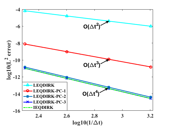
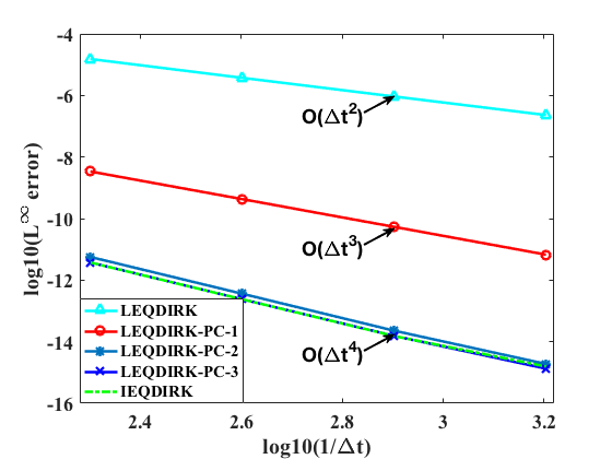
(a) $L^{2}$ and $L^{\infty}$ errors using the DIRK4th scheme

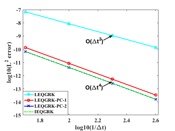
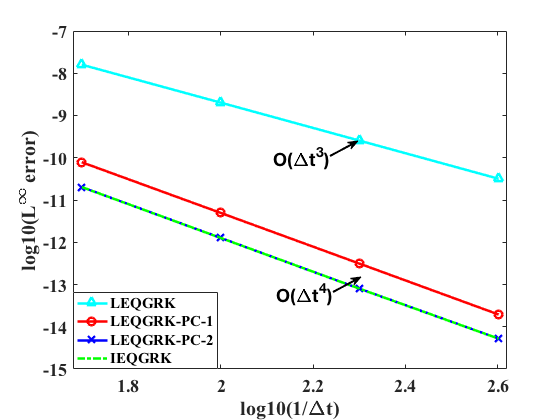
(b) $L^{2}$ and $L^{\infty}$ errors using the Gauss4th scheme

Figure 4.1: Time step refinement tests with the proposed numerical schemes for the Cahn-Hilliard equation.

To further compare the DIRK4th and Gauss4th schemes, we summarize their $L^{2}$ and $L^{\infty}$ errors in the same plot, as shown in Figure 4.2(a)-(b), respectively. We observe that the Gauss4th scheme reaches its order of accuracy even with a larger time step size. After a few iterations, the DIRK4th scheme also reaches its order of accuracy quickly. Also, with the same time step size, the Gauss4th scheme is more accurate than the DIRK4th scheme.

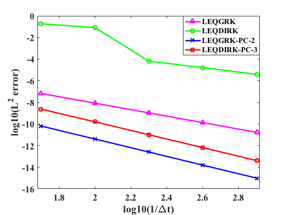
(a) $L^{2}$ error

(b) $L^{\infty}$ error

Figure 4.2: $L^{2}$ and $L^{\infty}$ errors using DIRK4th and Gauss4th schemes for the Cahn-Hilliard equation.

To further benchmark these two schemes, we conduct several numerical tests. For comparison, we also implement the widely used 2nd order convex splitting scheme (which we refer to as the 2nd-CS scheme in this paper),

$$\frac{\phi^{n+1}-\phi^{n}}{\Delta t}=\lambda\Delta\Big{[}-\varepsilon^{2}\Delta\phi^{n+\frac{1}{2}}+\frac{1}{2}((\phi^{n})^{2}+(\phi^{n+1})^{2})\phi^{n+\frac{1}{2}}-(\frac{3}{2}\phi^{n}-\frac{1}{2}\phi^{n-1})\Big{]}.$$ (4.10)

We emphasis that there is no theoretical proofs for energy dissipation for the 2nd-CS scheme above, though it is more accurate than the first-order convex splitting scheme.

For the first example, we choose the domain as $[0\,\,\,1]^{2}$, and parameters $\lambda=1$, $\epsilon=0.01$, and $\gamma=1$. Then, we use the initial condition [34]

$$\phi(x,y,t=0)=0.05\Big{(}\cos(3x)\cos(4y)+(\cos(4x)\cos(3y))^{2}+\cos(x-5y)\cos(2x-y)\Big{)}.$$ (4.11)

This initial profile would drive a fast coarsening dynamics, such that the algorithm would predict ’wrong’ dynamics if it is not accurate or robust enough. In this example, we intend to find the maximum possible time step that one can capture the correct dynamics numerically. Various numerical schemes with different time steps are implemented and compared. The numerical results are summarized in Figure 4.3, where the predicted profile of $\phi(x,y)$ at $t=0.1$ are shown using different schemes and time-step sizes. We observe that the maximum possible time step size for the 2nd-order convex splitting scheme is approximately $\Delta t=6.25\times 10^{-5}$. For the DIRK4th scheme with 5 prediction iterations, the maximum time step size is approximately $\Delta t=1.25\times 10^{-4}$. For the Gauss4th method with five prediction iterations, it is $2.5\times 10^{-4}$. Notice, the prediction steps could be easily solved with FFT, so the computational cost is negligible compared to the correction step.

These results indicate that the DIRK4th and Gauss4th schemes are superior over the 2nd order convex splitting scheme in this simulation. In addition, one should notice that there is no theoretical guarantee of monotonic energy decay with the 2nd order convex splitting scheme, and the implementation of the convex splitting scheme is relatively complicated, as nonlinear equations have to be solved at each time step. In contrast, the proposed high-order schemes here are linear and easy to implement. Also, they are rather general so that they can be applied to a broad class of gradient flow models.

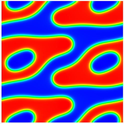
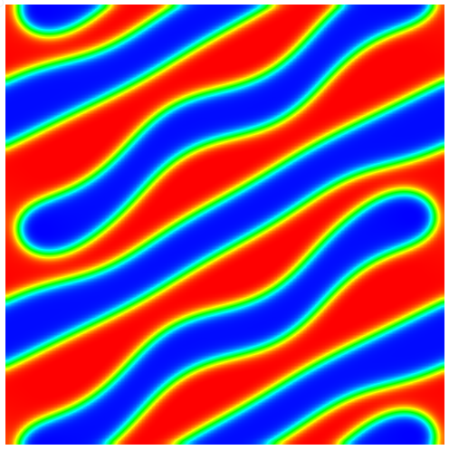
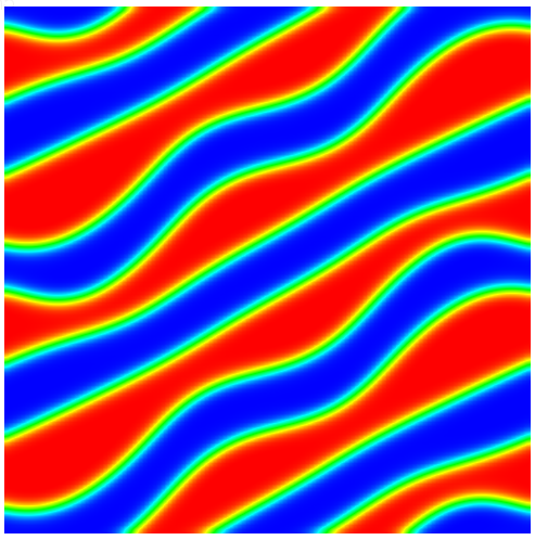
(a) The profile of $\phi$ at $t=0.1$ using various time step sizes: $\Delta t=2.5\times 10^{-4},1.25\times 10^{-4},3.125\times 10^{-5}$ with the 2nd-order convex splitting scheme.

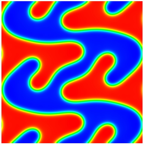
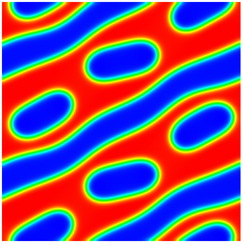
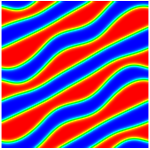
(b) The profile of $\phi$ at $t=0.1$ using various time step sizes: $\Delta t=5\times 10^{-4},2.5\times 10^{-4},1.25\times 10^{-4}$ with the DIRK4th scheme.

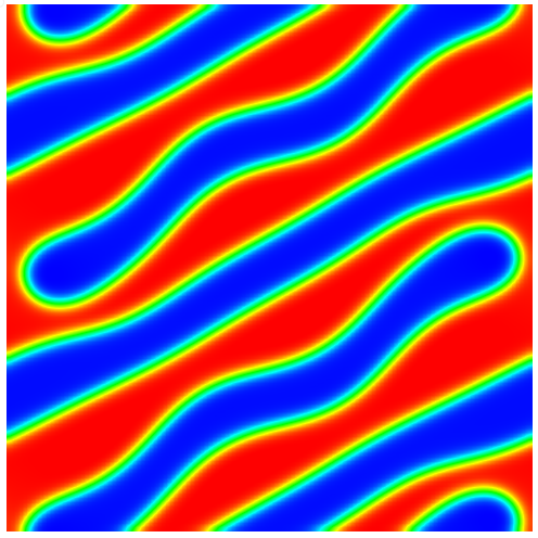
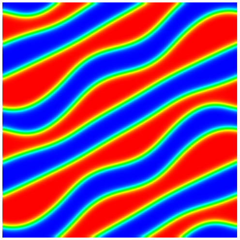
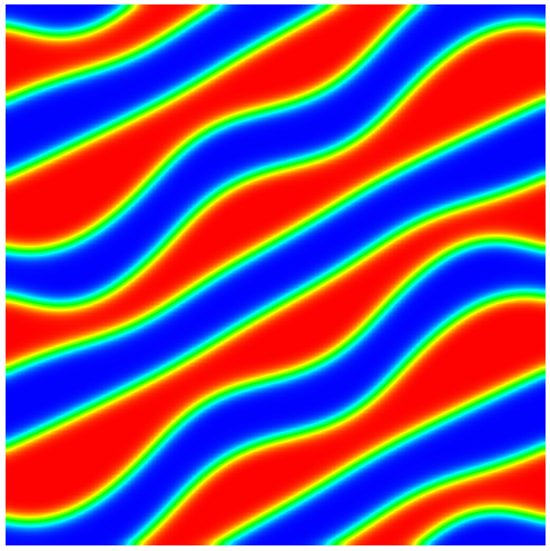
(c) The profile of $\phi$ at $t=0.1$ using various time step sizes: $\Delta t=5\times 10^{-4},2.5\times 10^{-4},1.25\times 10^{-4}$ with the Gauss4th scheme.

Figure 4.3: A comparison of the three schemes on predicting accurate Cahn-Hilliard dynamics at various time step sizes. The figures show the numerical results of $\phi$ at time $t=0.1$ using different schemes with various time steps. The last sub-figure in each row indicates the maximum possible time step size to predict correct dynamics for the corresponding scheme. Both the DIRK4th scheme and the Gauss4th scheme perform better than the 2nd order CS scheme.

To further confirm these findings, we conduct an additional numerical experiment with random initial conditions. Specifically, we use

$$\phi(x,y,t=0)=0.001\textrm{rand}(x,y),$$ (4.12)

where $\textrm{rand}(x,y)$ generates random numbers between $-1$ and $1$ uniformly. The rest settings are kept the same as in the previous example. The numerical results are summarized in Figure 4.4. This numerical example also indicates that the new schemes allow larger step sizes for accurately predicting the coarsening dynamics over the 2nd CS scheme.

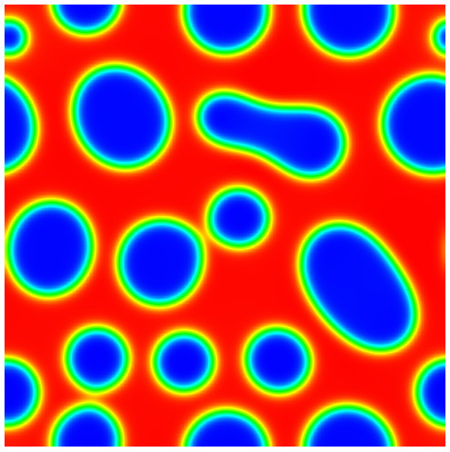
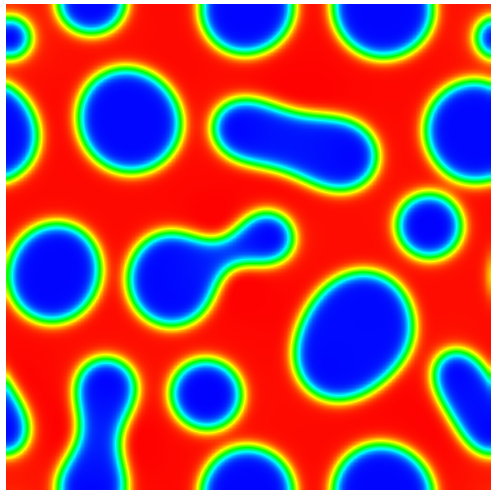
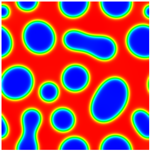
(a) The profile of $\phi$ at $t=0.1$ using various time step sizes: $\Delta t=2.5\times 10^{-4},1.25\times 10^{-4},6.25\times 10^{-5}$ with the 2nd order convex splitting method

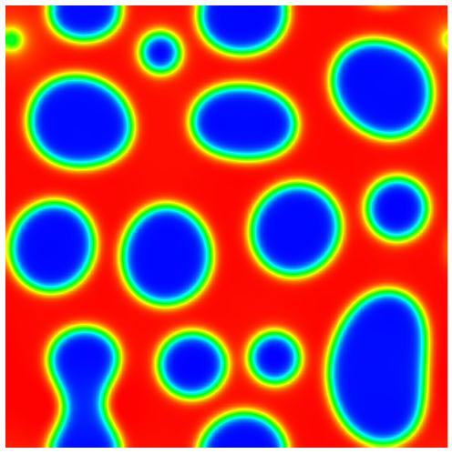
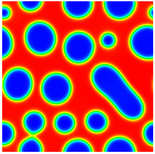
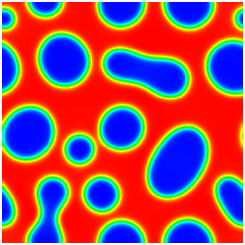
(b) The profile of $\phi$ at $t=0.1$ using various time step sizes: $\Delta t=5\times 10^{-4},2.5\times 10^{-4},1.25\times 10^{-5}$ with the DIRK4th method.

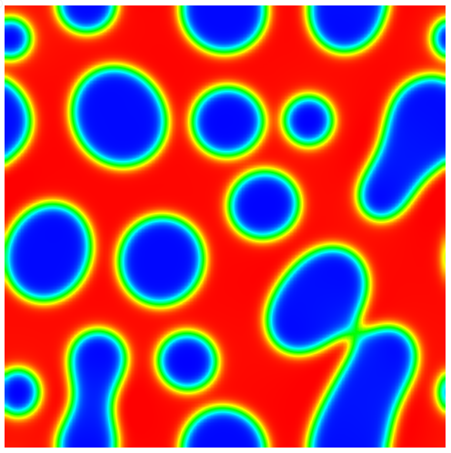
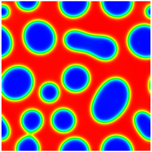
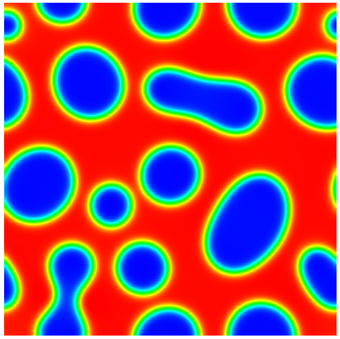
(c) The profile of $\phi$ at $t=0.1$ using various time step sizes: $\Delta t=5\times 10^{-4},2.5\times 10^{-4},1.25\times 10^{-5}$ with the Gauss4th method.

Figure 4.4: A comparison of the three schemes on predicting accurate Cahn-Hilliard dynamics with random initial conditions. These figures show the numerical results of $\phi$ at time $t=0.1$ using different schemes with various time steps. The last sub-figure in each row indicates the maximum possible time step size to predict correct dynamics for the corresponding scheme. The Gauss4th scheme performs the best.

4.2 Molecular beam epitaxial growth model

In this subsection, we focus on the molecular beam epitaxial growth model with slope selection given as follows

$$\phi_{t}=-\lambda\Big{(}\varepsilon^{2}\Delta^{2}\phi-\nabla\cdot\big{(}(|\nabla\phi|^{2}-1)\nabla\phi\big{)}\Big{)},$$ (4.13)

where the free energy functional is given by

$$F=\dfrac{\varepsilon^{2}}{2}\|\Delta\phi\|^{2}+\frac{1}{4}\big{\|}|\nabla\phi|^{2}-1\big{\|}^{2}.$$ (4.14)

We let $q=\frac{1}{2}\big{(}|\nabla\phi|^{2}-1-\gamma\big{)}$ and rewrite the energy functional as

$$\mathcal{F}=\frac{1}{2}\Big{(}\phi,\varepsilon^{2}\Delta^{2}\phi-\gamma\Delta\phi\Big{)}+\|q\|^{2}-\frac{\gamma^{2}+2\gamma}{4}|\Omega|.$$ (4.15)

Using the EQ reformulation, we have the following equivalent system

$$\begin{cases}\phi_{t}=-\lambda\Big{(}\varepsilon^{2}\Delta^{2}\phi-\gamma\Delta\phi-\nabla\cdot\big{(}2q\nabla\phi\big{)}\Big{)},\\ q_{t}=\nabla\phi\cdot\nabla\phi_{t},\end{cases}$$ (4.16)

with the consistent initial condition

$$\begin{cases}\phi(t=0)=\phi_{0},\\ q(t=0)=\frac{1}{2}\big{(}|\nabla\phi_{0}|^{2}-1-\gamma\big{)}.\end{cases}$$ (4.17)

It is readily to show that new system (4.16) obeys the following energy dissipation law

$$\frac{d\mathcal{F}}{dt}=-\lambda\Big{\|}\varepsilon^{2}\Delta^{2}\phi-\gamma\Delta\phi-\nabla\cdot\big{(}2q\nabla\phi\big{)}\Big{\|}^{2}\leq 0.$$ (4.18)

Applying the LEQRK-PC scheme for system (4.16), we have the following scheme.

Scheme 4.2.

Let $b_{i}$, $a_{ij}$ ($i,j=1,\cdots,s$) be real numbers and let $c_{i}=\sum\limits_{j=1}^{s}a_{ij}$. For given $(\phi^{n},q^{n})$ and $\Phi_{N}(t_{n}+c_{i}\Delta t),Q_{N}(t_{n}+c_{i}\Delta t),\forall i$, the following intermediate values are first calculated by the following prediction-correction strategy

1. Prediction: we set $\Phi_{i}^{n,0}=\Phi_{N}(t_{n}+c_{i}\Delta t),$ $Q_{i}^{n,0}=Q_{N}(t_{n}+c_{i}\Delta t)$ and $M>0$ as a given integer. For $m=0$ to $M-1$, we compute $\Phi_{i}^{n,m+1}$, $k_{i}^{n,m+1}$, $l_{i}^{n,m+1}$, $Q_{i}^{n,m+1}$ using

   $$\left\{\begin{array}[]{l}\Phi_{i}^{n,m+1}=\phi^{n}+\Delta t\sum\limits_{j=1}^{s}a_{ij}k_{j}^{n,m+1},\\ k_{i}^{n,m+1}=-\lambda\Big{(}\varepsilon^{2}\Delta^{2}\Phi_{i}^{n,m+1}-\gamma\Delta\Phi_{i}^{n,m+1}-\nabla\cdot\big{(}2Q_{i}^{n,m}\nabla\Phi_{i}^{n,m}\big{)}\Big{)},\\ l_{i}^{n,m+1}=\nabla\Phi_{i}^{n,m+1}\cdot\nabla k_{i}^{n,m+1},\\ Q_{i}^{n,m+1}=q^{n}+\Delta t\sum\limits_{j=1}^{s}a_{ij}l_{j}^{n,m+1},\end{array}\right.\quad i=1,\cdots,s.$$ (4.19)

   Given the error tolerance $TOL>0$, if $\max\limits_{i}\|\Phi^{n,m+1}_{i}-\Phi^{n,m}_{i}\|_{\infty}<TOL$, we stop the iteration and set $\Phi^{n,*}_{i}=\Phi_{i}^{n,m+1}$; otherwise, we set $\Phi^{n,*}_{i}=\Phi_{i}^{n,M}$.

2. Correction: for the predicted $\Phi^{n,*}_{i}$, we compute the intermediate values $\Phi_{i}^{n},Q_{i}^{n},k_{i}^{n},l_{i}^{n}$ via

   $$\left\{\begin{array}[]{l}\Phi_{i}^{n}=\phi^{n}+\Delta t\sum\limits_{j=1}^{s}a_{ij}k_{j}^{n},\\ Q_{i}^{n}=q^{n}+\Delta t\sum\limits_{j=1}^{s}a_{ij}l_{j}^{n},\\ k_{i}^{n}=-\lambda\Big{(}\varepsilon^{2}\Delta^{2}\Phi_{i}^{n}-\gamma\Delta\Phi_{i}^{n}-\nabla\cdot\big{(}2Q_{i}^{n}\nabla\Phi_{i}^{n,*}\big{)}\Big{)},\\ l_{i}^{n}=\nabla\Phi_{i}^{n,*}\cdot\nabla k_{i}^{n},\end{array}\right.\quad i=1,\cdots,s.$$ (4.20)

Then $(\phi^{n+1},q^{n+1})$ is updated via

$$\phi^{n+1}=\phi^{n}+\Delta t\sum\limits_{i=1}^{s}b_{i}k_{i}^{n},$$ (4.21)

$$q^{n+1}=q^{n}+\Delta t\sum\limits_{i=1}^{s}b_{i}l_{i}^{n}.$$ (4.22)

We apply the proposed arbitrarily high order schemes to solve MBE model (4.13). We repeat the time step refinement test first. Here we use domain $[0\,\,\,2\pi]^{2}$ and choose parameters $\lambda=0.01$, $\gamma=1$ and $\varepsilon=1$. By adding the proper force term on the right-hand side of the equation, we create the real solution

$$\phi(x,y,t)=\sin(x)\sin(y)\cos(t).$$ (4.23)

for the MBE model. Then we solve the modified model in the domain with a periodic boundary using the pseudo-spectral method for spatial discretization on $128^{2}$ meshes. The $L^{2}$ errors and $L^{\infty}$ errors using different schemes and various time steps are summarized in Figure 4.5. Here we observe similar results, i.e., the DIRK4th scheme reaches 2nd order accuracy without prediction, but obtain 4th order accuracy with only two iteration steps for both the $L^{2}$ and $L^{\infty}$ norms. This is due to the low-order approximation for extrapolating the explicit terms. Analogously, the Gauss4th scheme is 3rd order accurate without any prediction steps and reaches 4th order accuracy with one iteration step.

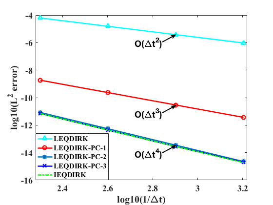
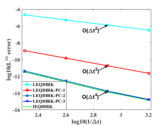
(a) $L^{2}$ and $L^{\infty}$ errors using the DIRK4th scheme

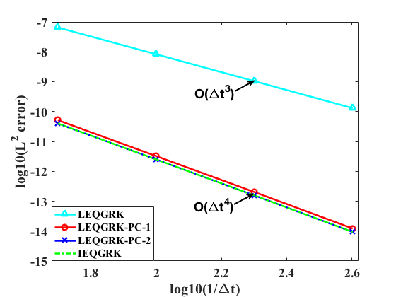
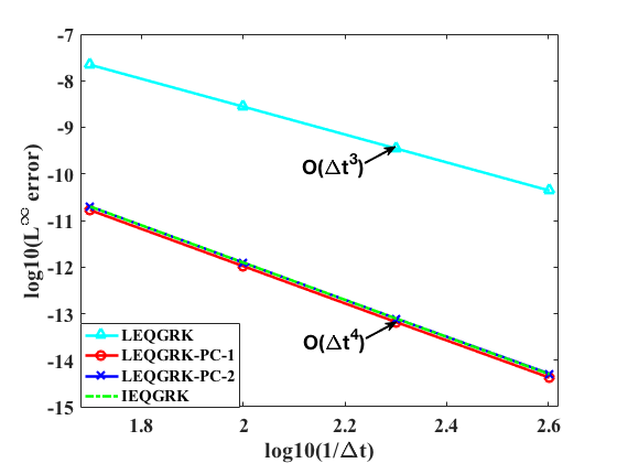
(b) $L^{2}$ and $L^{\infty}$ errors using the Gauss4th scheme

Figure 4.5: Time step refinement tests with the proposed numerical schemes for the MBE model.

To compare the accuracy of the DIRK4th scheme with that of the Gauss4th scheme in solving the molecular beam epitaxy (MBE) model, we summarize their $L^{2}$ and $L^{\infty}$ errors in the same figure as shown in 4.6. We observe that the Gauss4th method has smaller errors than the DIRK4th scheme if using the same time step sizes.

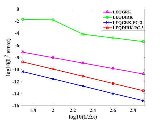
(a) $L^{2}$ errors

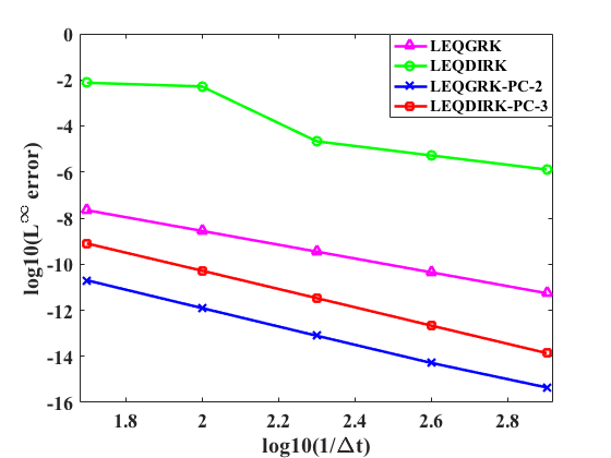
(b) $L^{\infty}$ errors

Figure 4.6: $L^{2}$ and $L^{\infty}$ errors using the DIRK4th method and the Gauss4th method for the MBE model.

Next, we use the proposed DIRK4th and Gauss4th schemes to solve two benchmark problems associated to the MBE model (4.13). As before, we introduce the 2nd-order convex splitting scheme

$$\frac{\phi^{n+1}-\phi^{n}}{\delta t}=-\lambda\Big{(}\varepsilon^{2}\Delta^{2}\phi^{n+\frac{1}{2}}-\frac{1}{2}\nabla\cdot\big{(}(|\nabla\phi^{n+1}|^{2}+|\nabla\phi^{n}|^{2})\nabla\phi^{n+\frac{1}{2}}\big{)}+\Delta(\frac{3}{2}\phi^{n}-\frac{1}{2}\phi^{n-1})\Big{)},$$ (4.24)

which will be used for comparison with the proposed linear high-order schemes.

Following [34], we choose the domain as $[0\,\,\,2\pi]^{2}$, parameters $\lambda=1$, $\varepsilon^{2}=0.1$, and $\gamma=1$. We solve the MBE model in a periodic domain using the pseudo-spectral method with $128^{2}$ meshes. All the numerical schemes (i.e., the DIRK4th, Gauss4th, and 2nd CS scheme) are implemented. Five prediction iterations are used for both the DIRK4th and Gauss4th scheme. The energy from $t=0$ to $t=15$ are calculated with different time steps and the results are summarized in Figure 4.7. We observe the maximum time steps to obtain accurate solutions are $\Delta t=0.015625$ for 2nd order convex splitting scheme, $\Delta t=0.0025$ for LEQDIRK-PC-5, and $\Delta t=0.015625$ for LEQGRK-PC-5.

We emphasis that, using the 2nd-order convex splitting scheme (4.24) for the MBE model, nonlinear equations have to be solved at each time step, but DIRK and Gauss scheme are all linear and easy to implement. In addition, for the 2nd order convex splitting scheme, there are no theoretical proofs for energy dissipation, but the high-order linear schemes introduced in this paper all guarantee energy dissipation laws.

(a) Convex splitting scheme

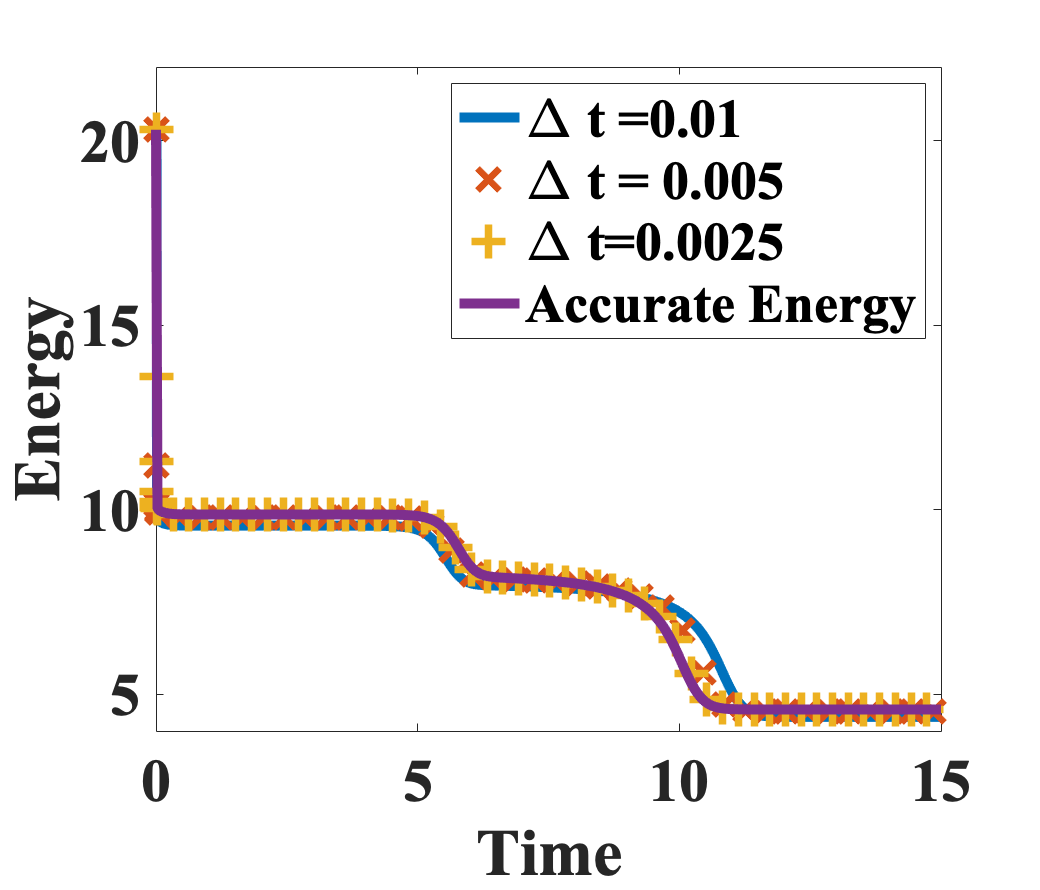
(b) LEQDIRK-PC-5

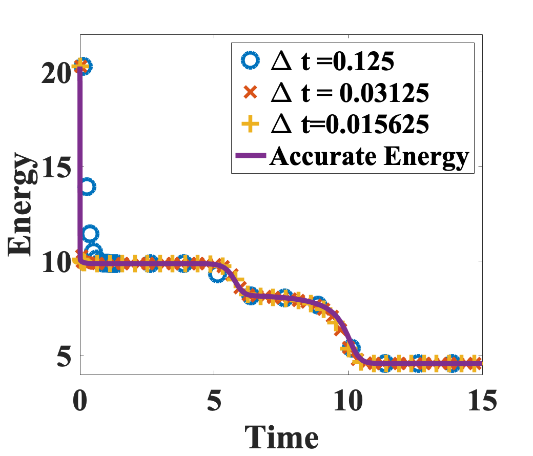
(c) LEQGRK-PC-5

Figure 4.7: Numerical results of energy evolution for the MBE model using different schemes with various time steps.

With the proposed high-order schemes, we can easily solve the MBE model with relatively larger time steps in most cases, making simulating long-time dynamics practical. Here we give an additional example as an illustration. We choose the domain as $[0\,\,\,12.8]^{2}$ and $\varepsilon=0.03$. The rest parameters are the same as in previous examples. We use $256^{2}$ meshes. It is known that the MBE coarsening dynamics follows a power law, where the energy decreases as $O(t^{-\frac{1}{3}})$, and the roughness increases as $O(t^{\frac{1}{3}})$ [34]. The numerical results are summarized in Figure 4.8, showing a strong agreement with the expected power law.

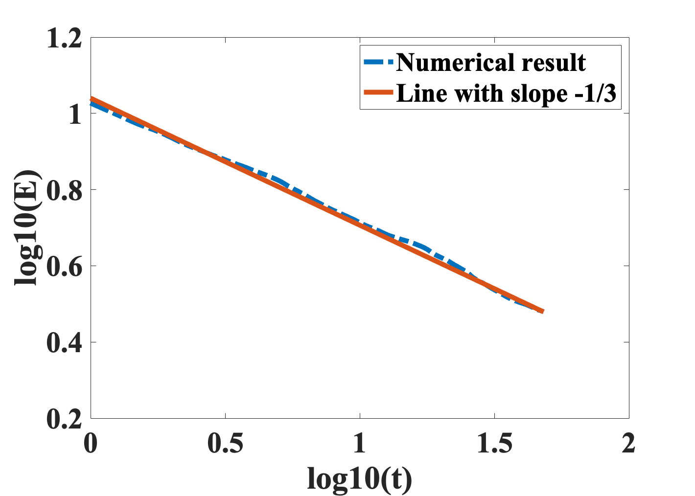
(a) Energy

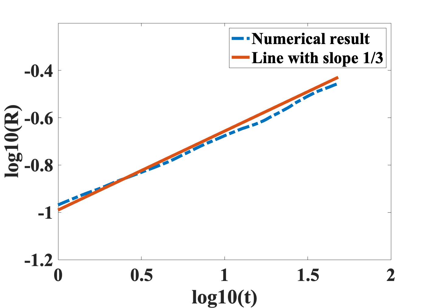
(b) Rougness

Figure 4.8: The numerical results show proper power law dynamics for the decreasing energy as $O(t^{-1/3})$ and increasing roughness as $O(t^{1/3})$.

The profile of $\phi$ and $\Delta\phi$ at different times are summarized in Figure 4.9 and 4.10, respectively. These profiles look qualitatively similar to the reported results. These results strongly support our claim that the general arbitrarily high order linear schemes can be applied to predict accurate dynamics for the MBE model.

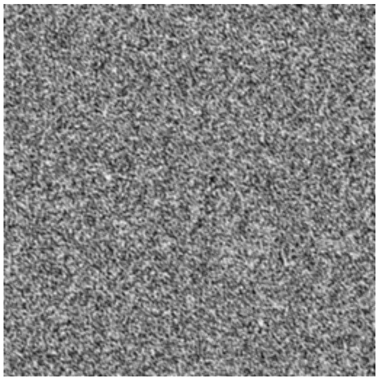
(a) $\phi$ at $t=0$

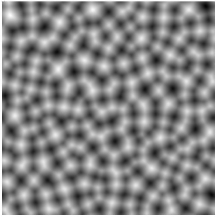
(b) $\phi$ at $t=5$

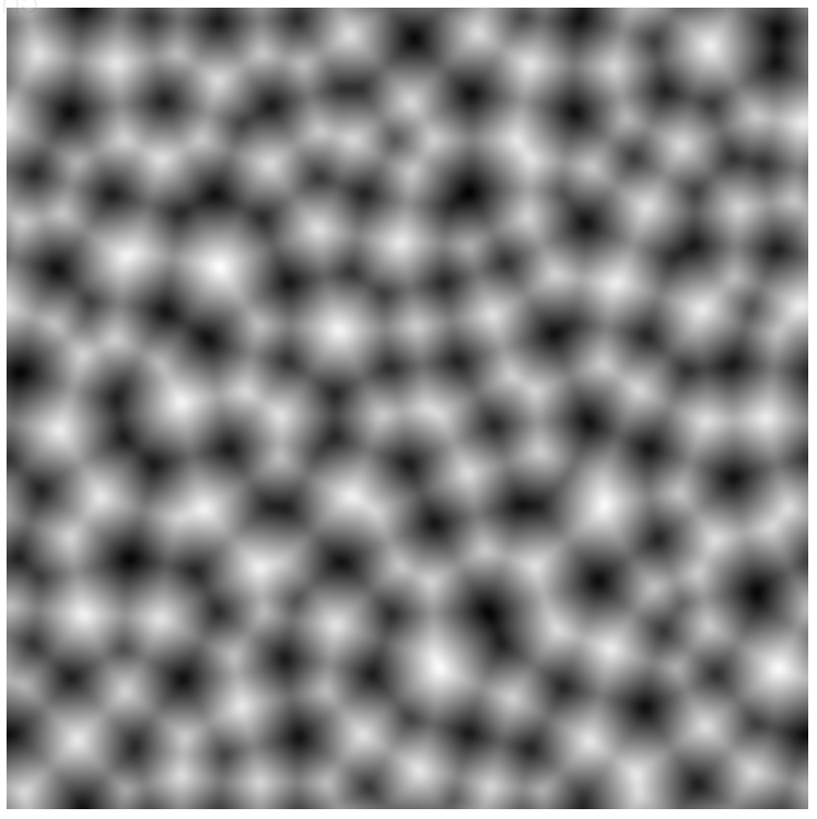
(c) $\phi$ at $t=10$

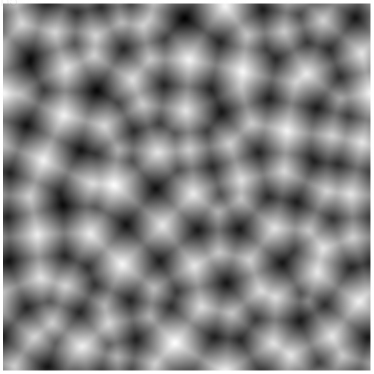
(d) $\phi$ at $t=20$

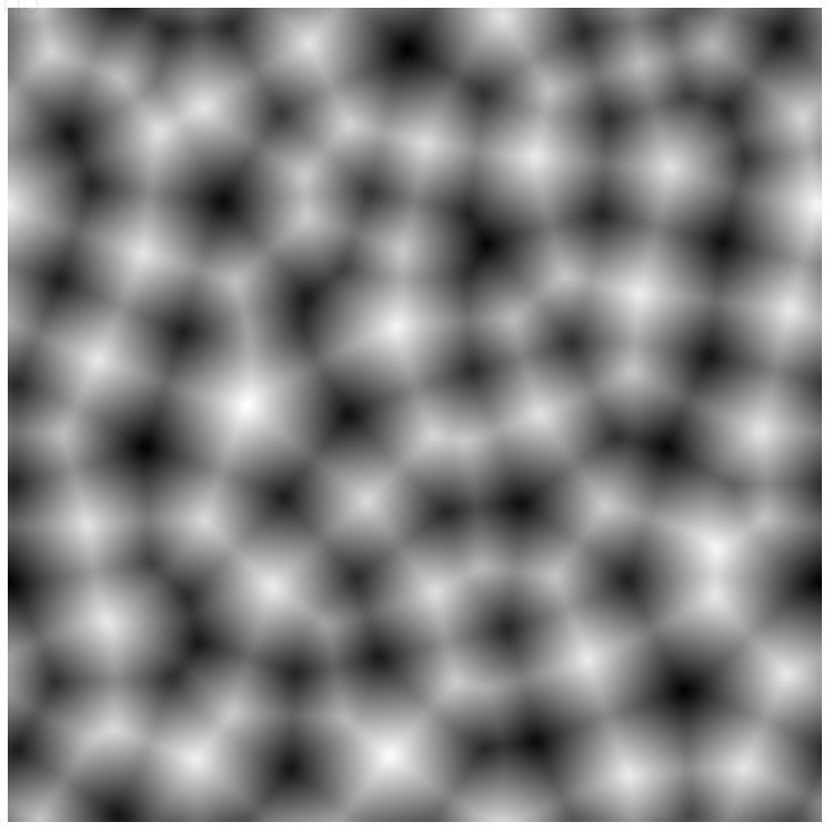
(e) $\phi$ at $t=30$

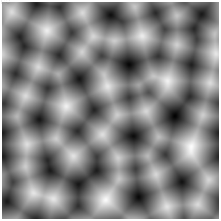
(f) $\phi$ at $t=45$

Figure 4.9: The profile of $\phi$ at different times.

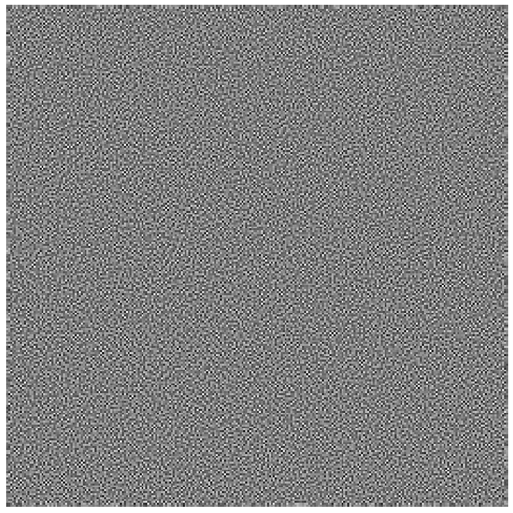
(a) $\Delta\phi$ at $t=0$

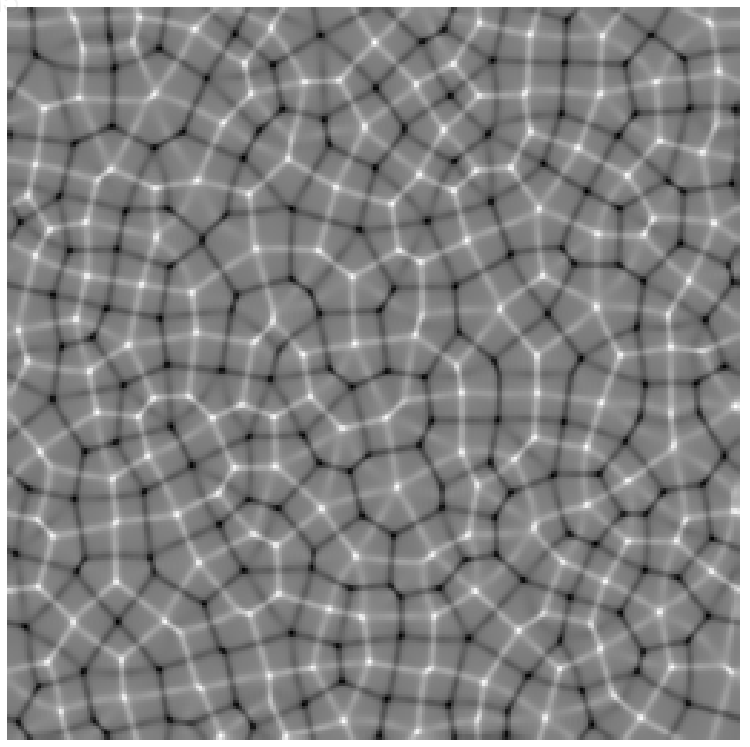
(b) $\Delta\phi$ at $t=5$

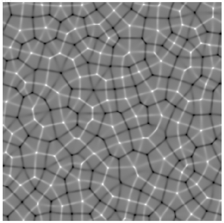
(c) $\Delta\phi$ at $t=10$

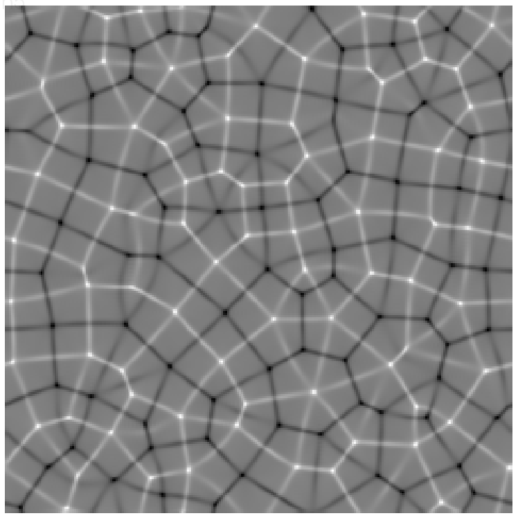
(d) $\Delta\phi$ at $t=20$

(e) $\Delta\phi$ at $t=30$

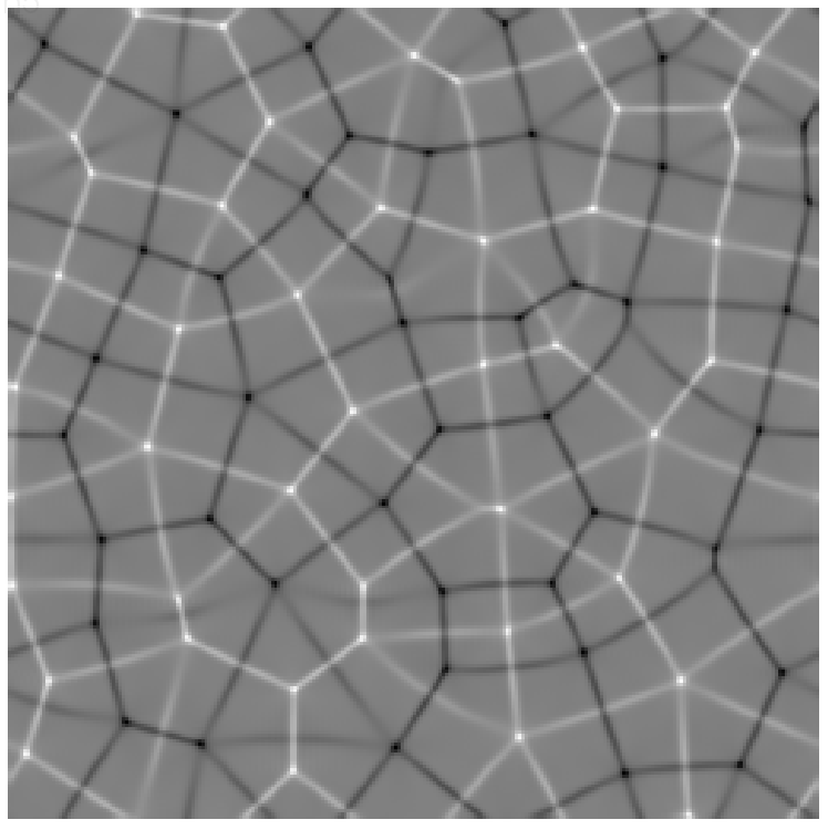
(f) $\Delta\phi$ at $t=45$

Figure 4.10: The profile of $\Delta\phi$ at different times.

5 Conclusions

In this paper, we present a new paradigm for developing arbitrarily high order, fully discrete numerical algorithms. These newly proposed algorithms have several advantageous properties: (1) the schemes are all linear such that they are easy to implement and computationally efficient; (2) the schemes are unconditionally energy stable and uniquely solvable such that large time steps can be used in some long-time dynamical simulations; (3) the schemes can reach arbitrarily high-order of accuracy spatial-temporally such that relatively large meshes can guarantee the desired accuracy of numerical solutions; (4) the schemes do not depend on the specific expression of the free energy explicitly such that it can be readily applied to a large class of general gradient flow models. The proofs for energy stability and uniquely solvability are given, and numerical tests with benchmark problems are shown to illustrate the effectiveness of the proposed schemes.

References

- [1] J. W. Barrett, J. F. Blowey, and H. Garcke. On fully practical finite element approximations of degenerate cahn-hilliard systems. ESAIM: M2AN, 35:713–748, 2001.
- [2] K. Burrage and J. C. Butcher. Stability criteria for implicit Runge-Kutta methods. SIAM Journal on Numerical Analysis, 16(1):46–57, 1979.
- [3] J. W. Cahn and S. M. Allen. A microscopic theory for domain wall motion and its experimental varification in fe-al alloy domain growth kinetics. J. Phys. Colloque, C7:C7–51, 1977.
- [4] J. W. Cahn and J. E. Hilliard. Free energy of a nonuniform system. I. interfacial free energy. Journal of Chemical Physics, 28:258–267, 1958.
- [5] L. Chen, J. Zhao, and X. Yang. Regularized linear schemes for the molecular beam epitaxy model with slope selection. Applied Numerical Mathematics, 128:138–156, 2018.
- [6] W. Chen, S. Conde, C. Wang, X. Wang, and S. Wise. A linear energy stable scheme for a thin film model without slope selection. Journal of Scientific Computing, 52:546–562, 2012.
- [7] Q. Cheng, X. Yang, and J. Shen. Efficient and accurate numerical schemes for a hydrodynamically coupled phase field diblock copolymer model. Journal of Computational Physics, 341:44–60, 2017.
- [8] S. Clarke and D. D. Vvedensky. Origin of reflection high-energy electron-diffraction intensity oscillations during molecular-beam epitaxy: A computational modeling approach. Phys. Rev. Lett., 58:2235–2238, 1987.
- [9] S. Dong, Z. Yang, and L. Lin. A family of second-order energy-stable schemes for cahn-hilliard type equations. Journal of Computational Physics, 383:24–54, 2019.
- [10] M. Elsey and B. Wirth. A simple and efficient scheme for phase field crystal simulation. ESAIM: M2AN, 47:1413–1432, 2013.
- [11] D. Eyre. Unconditionally gradient stable time marching the Cahn-Hilliard equation. Computational and mathematical models of microstructural evolution (San Francisco, CA, 1998), 529:39–46, 1998.
- [12] W. Feng, C. Wang, S. Wise, and Z. Zhang. A second-order energy stable backward differentiation formula method for the epitaxial thin film equation with slope selection. Numerical Methods for Partial Differential Equations, 34(6):1975–2007, 2018.
- [13] D. Furihata and T. Matsuo. Discrete variational derivative method. A structure-preserving numerical method for partial differential equations. CRC Press, 2011.
- [14] K. Glasner and S. Orizaga. Improving the accuracy of convexity splitting methods for gradient flow equations. Journal of Computational Physics, 315:52–64, 2016.
- [15] Y. Gong and J. Zhao. Energy-stable Runge-Kutta schemes for gradient flow models using the energy quadratization approach. Applied Mathematics Letters, 94:224–231, 2019.
- [16] Y. Gong, J. Zhao, and Q. Wang. Linear second order in time energy stable schemes for hydrodynamic models of binary mixtures based on a spatially pseudospectral approximation. Advances in Computational Mathematics, 44:1573–1600, 2018.
- [17] Y. Gong, J. Zhao, and Q. Wang. Second order fully discrete energy stable methods on staggered grids for hydrodynamic phase field models of binary viscous fluids. SIAM Journal on Scientific Computing, 40(2):B528–B553, 2018.
- [18] Y. Gong, J. Zhao, and Q. Wang. Arbitrarily high-order unconditionally energy stable sav schemes for gradient flow models. ArXiv, pages 1–22, 2019.
- [19] Y. Gong, J. Zhao, and Q. Wang. Arbitrary high order energy stable schemes for gradient flow models based on energy quadratization. SIAM Journal on Scientific Computing, page accepted, 2019.
- [20] F. Guillen-Gonzalez and G. Tierra. Second order schemes and time-step adaptivity for Allen-Cahn and Cahn-Hilliard models. Computers Mathematics with Applications, 68(8):821–846, 2014.
- [21] Z. Guo, P. Lin, J. Lowengrub, and S. Wise. Mass conservative and energy stable finite difference methods for the quasi-incompressible navier-stokes-cahn-hilliard system: primitive variable and projection-type schemes. Computer Methods in Applied Mechanics and Engineering, 326:144–174, 2017.
- [22] D. Hou, M. Azaiez, and C. Xu. A variant of scalar auxiliary variable approaches for gradient flows. Journal of Computational Physics, 395:307–332, 2019.
- [23] W. Hu and M. lai. Unconditionally energy stable immersed boundary method with application to vesicle dyanmics. East Asian Journal on Applied Mathematics, 3(3):247–262, 2013.
- [24] J. Kim, K. Kang, and J. Lowengrub. Conservative multigrid methods for ternary cahn-hilliard systems. Commun. Math. Sci., 2:53–77, 2004.
- [25] Z. Liu and X. Li. Efficient modified techniques of invariant energy quadratization approach for gradient flows. Applied Math. Letters, 98:206–214, 2019.
- [26] F. Luo, H. Xie, M. Xie, and F. Xu. Adaptive time-stepping algorithms for molecular beam epitaxy: based on energy or roughness. Applied Mathematics Letters, 99:105991, 2020.
- [27] Z. Qiao, Z. Sun, and Z. Zhang. Stability and convergence of second-order schemes for the nonlinear epitaxial growth model without slope selection. Mathematics of Computation, 84(292):653–674, 2015.
- [28] Z. Qiao, Z. Zhang, and Tao Tang. An adaptive time-stepping strategy for the molecular beam epitaxy models. SIAM Journal on Scientific Computing, 33(3):1395–1414, 2011.
- [29] J. Shen and J. Xu. Stabilized predictor-corrector schemes for gradient flows with strong anisotropic free energy. Communications in Computational Physics, 24(3):635–654, 2018.
- [30] J. Shen, J. Xu, and J. Yang. The scalar auxiliary variable (sav) approach for gradient flows. Journal of Computational Physics, 353:407–416, 2018.
- [31] J. Shen, J. Xu, and J. Yang. A new class of efficient and robust energy stable schemes for gradient flows. SIAM Review, 61(3):474–506, 2019.
- [32] J. Shen and X. Yang. Numerical approximations of Allen-Cahn and Cahn-Hilliard equations. Disc. Conti. Dyn. Sys.-A, 28:1669–1691, 2010.
- [33] C. Theng, I. Chern, and M. Lai. Simulating binary fluid-surfactant dynamics by a phase field model. Discrete and Continuous Dynamical Systems B, 17(4):1289–1307, 2012.
- [34] C. Wang, X. Wang, and S. Wise. Unconditionally stable schemes for equations of thin film epitaxy. Discrete and Continuous Dynamic Systems, 28(1):405–423, 2010.
- [35] S.-L. Wang, R.F. Sekerka, A.A. Wheeler, B.T. Murray, S.R. Coriell, R.J. Braun, and G.B. McFadden. Thermodynamically-consistent phase-field models for solidification. Physica D, 69:189–200, 1993.
- [36] S. Wise, J. Kim, and J. Lowengrub. Solving the regularized strongly anisotropic cahn-hilliard equation by an adaptive nonlinear multigrid method. Journal of Computational Physics, 226(1):414–446, 2007.
- [37] S. Wise, C. Wang, and J. S. Lowengrub. An energy-stable and convergent finite-difference scheme for the phase field crystal equation. SIAM Journal of Numerical Analysis, 47(3):2269–2288, 2009.
- [38] Z. Xu, X. Yang, H. Zhang, and Z. Xie. Efficient and linear schemes for anisotropic Cahn-Hilliard model using the stabilized-invariant energy quadratization (S-IEQ) approach. Computer Physics Communications, 238:36–49, 2019.
- [39] X. Yang. Linear, first and second-order, unconditionally energy stable numerical schemes for the phase field model of homopolymer blends. Journal of Computational Physics, 327:294–316, 2016.
- [40] X. Yang and L. Ju. Efficient linear schemes with unconditional energy stability for the phase field elastic bending energy model. Journal of Computational Physics, 315:691–712, 2017.
- [41] X. Yang, J. Zhao, and Q. Wang. Numerical approximations for the molecular beam epitaxial growth model based on the invariant energy quadratization method. J. Comput. Phys., 333:104–127, 2017.
- [42] X. Ye. The Legendre collocation method for the cahn-hilliard equation. Journal of Computational and Applied Mathematics, 150:87–108, 2003.
- [43] Z. Zhang, Y. Ma, and Z. Qiao. An adaptive time-stepping strategy for solving the phase field crystal model. Journal of Computational Physics, 249:204–215, 2013.
- [44] J. Zhao, X. Yang, Y. Gong, X. Zhao, J. Li, X. Yang, and Q. Wang. A general strategy for numerical approximations of thermodynamically consistent nonequilibrium models-part I: Thermodynamical systems. International Journal of Numerical Analysis and Modeling, 15(6):884–918, 2018.