Large deviation of long time average for a stochastic process : an alternative method.

Abstract

We present here a simple method for computing the large deviation of long time average for stochastic jump processes. We show that the computation of the rate function can be reduced to that of a partial differential equation governing the evolution of the probability generating function. The long time limit of this equation, which in many cases can be easily obtained, leads naturally to the rate function.

I Introduction.

Markov stochastic processes are at the heart of many area of science, ranging from statistical and quantum physics to biology and economics(vankampen2007stochastic, ; gardiner2004handbook, ). Broadly speaking, for time continuous models, a Markovian system in a state $\mathbf{x}$ at time $t$ will transit to a state $\mathbf{y}$ at time $t+dt$ with a probability that depends only on $\mathbf{x},\mathbf{y}$ and $t$ ; in other words the system has no memory. By following many (ideally an infinite number) trajectories $\mathbf{x}(\tau)$, one can construct the probability $P(\mathbf{u},t)$, i.e. the relative number of trajectories that pass through state $\mathbf{u}$ at time $\tau$. $P(\mathbf{u},t)$ is the fundamental quantity that gives the most complete description of the studied system.

During the last thirty years, large deviation theory of stochastic processes has attracted a large number of investigation as a natural reformulation of statistical physics (for a review, see (touchette2009thelarge, )). More specifically, there has been a great interest in using the tools of large deviation theory for studying the fluctuation of time-additive quantities(touchette2018introduction, ). In this approach, an information $\mathbf{r}(T)$ is extracted from each trajectory of a Markov process, and a probability density $p(\mathbf{r},T)$ is constructed for this information. Usually, one is interested only in the long time limit ($T\rightarrow\infty)$. A most studied case is the time average of the original variable $\mathbf{x}$:

$$\bar{\mathbf{x}}(T)=\frac{1}{T}\int_{0}^{T}x(\tau)d\tau$$ (1)

For jump processes that are the object of this note, the sum in (1) involves the usual Riemann integral.

The purpose of the present note is to present a simple mathematical framework for computing the probability density of such stochastic time averaged quantities. The basic idea is to reduce the problem at hand to the resolution of a partial differential equation and extract it long time behavior. The mathematical tools are fairly standard and in many cases lead simply to the desired results, as it will be discussed below.

This note is organized as follow : in the next section, we recall, for self consistency, the basic concepts of discreet Markovian stochastic processes, their large deviation theory and the main idea behind the method we call dPGF$k$ that transforms the problem at hand into a partial differential equation (PDE). Section III is devoted to the application of the method to various well studied stochastic processes and some of its extensions. The final section is devoted to discussions of the methods limitations and conclusion. The appendices handle the details of technical computations.

II the dPGF$k$ method.

We consider here first, for the sake of simplicity, one step Markovian jump processes of the stochastic variable $n$ ($=0,1,...$). These processes are described by their transition probabilities $W(n\rightarrow n\pm 1)=W^{\pm}(n)$. The probability $P(n,t)$ of being in state $n$ at time $t$ is governed by the Master equation(gardiner2004handbook, ; vankampen2007stochastic, )

$$\frac{\partial P(n,t)}{\partial t} = W^{+}(n-1)P(n-1,t)-W^{+}(n)P(n,t)$$ (2)

$$+ W^{-}(n+1)P(n+1,t)-W^{-}(n)P(n,t)$$

The above equation can be presented in the matricial form

$$\partial_{t}\left|P(t)\right\rangle={\cal L}\left|P(t)\right\rangle$$ (3)

where the (right, column) vector $\left|P(t)\right\rangle=(P(0,t),P(1,t),...)^{T}$ and the matrix ${\cal L}$ collects the rates of equation (2):

$${\cal L}_{n\pm 1}^{n}=W^{\pm}(n)\,\,\,\,;\,\,\,{\cal L}_{n}^{n}=-\left(W^{+}(n)+W^{-}(n)\right)$$

where the upper (lower) index designates the row (column) of the matrix. We suppose that the stochastic process has a stationary equilibrium state independent of the initial conditions.

The quantity of interest in this paper is the distribution of $\bar{n}(T),$ the long time average ($T\rightarrow\infty$) over a trajectory :

$$\bar{n}(T)=\frac{1}{T}\int_{0}^{T}n(t)dt$$

The Large Deviation theory states (touchette2009thelarge, ) that the probability density of $\bar{n}$ is given by

$${\cal P}\left(\bar{n}(T)=x\right)=e^{-TI(x)}$$

where the rate function $I(x)$ has its minimum and zero at $\mu=\left\langle n_{\text{eq}}\right\rangle$ of the original process.

To compute the rate function, which is the objective of the present note, the Donsker-Varadhan (DV)(donsker1975asymptotic, ; touchette2018introduction, ) method consists of (i) building the tilted matrix

$${\cal L}(k)={\cal L}+k{\cal D}$$ (4)

where ${\cal D}$ is a diagonal matrix such that its elements are$\left({\cal D}\right)_{m}^{n}=n\delta_{m}^{n}$ ; (ii) compute the largest eigenvalue of the above matrix: $\lambda(k)=\xi_{\text{max}}\left({\cal L}(k)\right)$ and (iii) compute the rate function $I(x)$ as the Legendre-Fenchel transform of $\lambda(k)$ :

$$I(x)=\underset{k}{\text{max}}\left(kx-\lambda(k)\right)$$ (5)

Note that the DV method is written for the Hermitian conjugate of ${\cal L}(k)$, but these two matrices have the same eigenvalues and therefore, without loss of generality, we use ${\cal L}(k)$ in this article.

We can use the usual tools of the trade of stochastic processes for the DV method. For any jump processes for example, we now that the matrix ${\cal L}$ has a (left,row) eigenvector $\left\langle 1\right|=(1,1,....)$ with eigenvalues $\lambda=0$, as applying this vector to both sides of equation (3) leads to

$$\partial_{t}\left\langle 1\right\rangle=\partial_{t}\left\langle 1|P\right\rangle=\left\langle 1|{\cal L}|P\right\rangle=0$$ (6)

which is another way of stating the obvious fact that $\partial_{t}\sum_{n}P(n,t)=0$. The right eigenvector associated with $\left\langle 1\right|$ is the equilibrium probabilities $\left|P_{\text{eq}}\right\rangle$. Various average quantities can be computed by applying an adequate left vector to equation (3). For example, the evolution of the mean is given by

$$\partial_{t}\left\langle n|P\right\rangle=\partial_{t}\left\langle n\right\rangle=\left\langle n|{\cal L}|P\right\rangle$$

where $\left\langle n\right|=(0,1,2,...)$. Simple manipulations of the sums involved show that

$$\partial_{t}\left\langle n\right\rangle=\left\langle W^{+}(n)-W^{-}(n)\right\rangle$$

The most complete information is contained in the probability generating function (PGF)

$$\phi(z,t)=\left\langle z^{n}\right\rangle=\sum_{n}z^{n}P(n,t)$$ (7)

and it is straightforward to show that(houchmandzadeh2010alternative, )

$$\partial_{t}\phi(z,t)=(z-1)\left\langle z^{n}W^{+}(n)\right\rangle+(1/z-1)\left\langle z^{n}W^{-}(n)\right\rangle$$ (8)

When the transition rates are polynomials in $n$, the $\left\langle...\right\rangle$ in the above expressions are reduced to derivatives of $\phi$. For example (see appendix A for more details), deriving expression (7) in respect to $z$, we have

$$\left\langle nz^{n}\right\rangle=z\frac{\partial\phi}{\partial z}\,\,\,;\,\,\,\left\langle n(n-1)z^{n}\right\rangle=z^{2}\frac{\partial^{2}\phi}{\partial z^{2}}$$

Therefore, the evolution of the PGF is governed by a partial differential equation on $\phi()$.

Now, we can embed the DV method into a similar problem by investigating the Master-like equation

$$\partial_{t}\left|P\right\rangle={\cal L}(k)\left|P\right\rangle$$ (9)

The vector $\left|P\right\rangle$ here is obviously not a probability anymore when $k\neq 0$, but for the purpose of computing the largest eigenvalue and the rate function, this is of no consequence. For example, for small $k$, we can solve equation (9) perturbatively by setting

$$\left|P(t)\right\rangle=\left(\left|P_{\text{0}}\right\rangle+k\left|P_{1}\right\rangle+k^{2}\left|P_{2}\right\rangle\right)e^{\left(k\eta_{1}+k^{2}\eta_{2}+...\right)t}$$ (10)

To the zero-th order of $k$ we have ${\cal L}\left|P_{0}\right\rangle=0$ so $\left|P_{0}\right\rangle$ is the equilibrium distribution $\left|P_{\text{eq}}\right\rangle$ of the original process. To the first order in $k$ we have

$$\eta_{1}\left|P_{0}\right\rangle={\cal L}\left|P_{1}\right\rangle+{\cal D}\left|P_{0}\right\rangle$$

Applying $\left\langle 1\right|$ to both side of the above equation, we obtain

$$\eta_{1}=\left\langle 1\right|{\cal D}\left|P_{0}\right\rangle=\left\langle n_{\text{eq}}\right\rangle$$

which, in other words, is the well known relation $\left.d\lambda(k)/dk\right|_{k=0}=\left\langle n_{\text{eq}}\right\rangle$.

More generally, defining the “PGF$k$” function $\phi$ as (and omitting to write the variable $k$ explicitly)

$$\phi(z,t)=\left\langle z^{n}|P\right\rangle=\left\langle z^{n}\right\rangle$$

its evolution is given by

$$\frac{\partial\phi(z,t)}{\partial t} = \left\langle z^{n}|{\cal L}|P\right\rangle+k\left\langle z^{n}|{\cal D}|P\right\rangle$$ (11)

$$= (z-1)\left\langle z^{n}W^{+}(n)\right\rangle+(1/z-1)\left\langle z^{n}W^{-}(n)\right\rangle$$

$$+ kz\frac{\partial\phi}{\partial z}$$

We see that compared to the original PGF, the evolution of the PGF$k$ adds only one first derivative to the original evolution equation. If we are able to compute the evolution of the PGF$k$ function, we automatically possess the largest eigenvalue of ${\cal L}(k)$. As we are only interested in the rate of long time evolution, in some cases as illustrated below, we don’t even need to solve the equation and we can restrict the investigation to some particular points, as we will discuss in the next section.

Note that we could approximate a jump process by a continuous Fokker Plank (FP) equation

$$\frac{\partial p}{\partial t}=-N\frac{\partial\left(ap\right)}{\partial x}+\frac{1}{2}\frac{\partial^{2}\left(bx\right)}{\partial x^{2}}$$

where $N$ is a natural scale of the problem used for discretization, $x=n/N$, $a(x)=\left(W^{+}(n)-W^{-}(n)\right)/N$, $b(x)=\left(W^{+}(n)+W^{-}(n)\right)/N$, and follow the classical tilted backward operator method reviewed by Touchette(touchette2018introduction, ). There are two disadvantages with this method : first, for discrete jump processes, the Fokker Plank approximation is of $O(1/N)$, which is a bad approximation if $N$ is not large ; second, the term $b(x)$ is usually not a constant and makes the backward, tilted FP operator rather intricate to investigate.

In the following, we illustrate the use of dPGF$k$ method through few simple cases and investigate some of its extensions.

III Applications and extensions

III.1 Simple chemical reactions.

Consider a simple chemical reaction $\emptyset\leftrightarrows A$ which models for example the production of RNA when a gene is active(paulsson2005modelsof, ). Denoting by $n$ the number of $A$ molecules, the transition rates are

$$W^{+}(n)=N\,\,\,;\,\,\,W^{-}(n)=n$$ (12)

Where the parameter $N$ (not necessarily an integer) is the production rate of $A$. The evolution of the PGF$k$ is given by

$$\frac{\partial\phi}{\partial t}=\left((k-1)z+1\right)\frac{\partial\phi}{\partial z}+N(z-1)\phi$$ (13)

We can, if needed, eliminate $N$ from the equation by setting $\phi=\exp(Nu)$.

At the point $z^{*}=1/(1-k)$, the prefactor of the $\partial_{z}\phi$ in equation (13) is zero ; therefore, at this point, $\phi(z^{*},t)$ evolves exponentially with rate

$$\lambda(k)=N(z^{*}-1)=N\frac{k}{1-k}$$ (14)

The Legendre transform of the above relation is

$$I(x)=\left(\sqrt{N}-\sqrt{x}\right)^{2}$$ (15)

This result has been obtained recently (zilber2019agiant, ) by using a WKB method.

If needed, we can check the above result by solving exactly equation (13) using the methods of characteristics : setting $\phi=\exp(Nu)$, the solution, for the initial condition $\phi(z,t=0)=1$ is :

$$u(z,t)=\frac{e^{(k-1)t}-1}{(k-1)^{2}}\left((k-1)z+1\right)+\frac{k}{1-k}t$$

The linear term in $t$ (up to the scaling factor $N)$ is indeed given by expression (14).

III.2 The Ehrenfest urn.

The Ehrenfest urn is one of the first simple stochastic processes used to understand the march toward equilibrium in statistical physics. The large deviation of its long-time average was investigated recently by Meerson and Zilber using a direct DV approach(meerson2018largedeviations, ). In this model, $N$ objects are distributed among two urns ; at exponentially distributed times, an object is drawn at random to change urn. Let $n$ designates the size of the first urn, then the transition rates for $n$ (up to a constant ) are given by:

$$W^{+}(n)=N-n\,\,\,;\,\,\,W^{-}(n)=n$$ (16)

According to relation (11), the evolution of the PGF$k$ is given by

$$\frac{\partial\phi}{\partial t}=N(z-1)\phi-(z^{2}-kz-1)\frac{\partial\phi}{\partial z}$$ (17)

which is a first order PDE. The system size $N$ can be eliminated by setting $\phi=u^{N}$, which transforms equation (17) into

$$\frac{\partial u}{\partial t}+(z^{2}-kz-1)\frac{\partial u}{\partial z}=(z-1)u$$ (18)

Consider $z_{\pm}$, the two roots of the algebraic equation

$$z^{2}-kz-1=0$$

where $z_{+}$ is the positive one. At $z=z_{\pm}$, the prefactor of $\partial_{z}u$ in equation (18) vanishes and we have

$$\frac{\partial u(z_{\pm},t)}{\partial t}=\left(z_{\pm}-1\right)u(z_{\pm},t)$$

As $z_{+}>z_{-}$, the largest eigenvalue of ${\cal L}(k)$ is simply

$$\lambda(k) = N(z_{+}-1)$$ (19)

$$= \frac{N}{2}\left(k-2+\sqrt{k^{2}+4}\right)$$

The fixed point method allows us to avoid solving the partial differential equation (18) ; however, as this is a first order linear PDE, it can be exactly solved. The solution of equation (18) for the initial condition $u(z,0)=1$ is

$$u(z,t)=\left((z-z_{-})e^{\lambda_{+}t}-(z-z_{+})e^{\lambda_{-}t}\right)/(z_{+}-z_{-})$$

where $\lambda_{\pm}=(z_{\pm}-1)$. Obviously, expression (19) is indeed the correct largest eigenvalue.

The Legendre transform of expression (19) is

$$I(x)=\left(N-2\sqrt{x(N-x)}\right)=\left(\sqrt{x}-\sqrt{N-x}\right)^{2}$$ (20)

Expression (19,20) were obtained by Meerson and Zilber (meerson2018largedeviations, ) using a direct DV approach.

The results of the above two subsections can be generalized. It can be shown by elementary algebra (see appendix B), that when rates are first order polynomials in $n$,

$$I(x)=\left(\sqrt{W^{+}(x)}-\sqrt{W^{-}(x)}\right)^{2}$$ (21)

this expression has been obtained by other methods in (zilber2019agiant, ).

We stress that this expression is only correct for single step processes with first order polynomial rates. In general, $I(x)$ must vanish for $x=\left\langle n_{\text{eq}}\right\rangle$ ; In expression (21) however, $I(x)$ vanishes at $x^{*}$ such that $W^{+}(x^{*})=W^{-}(x^{*})$. In general, $x^{*}\neq\left\langle n_{\text{eq}}\right\rangle$ and these two quantities coincide only for first order polynomial rates of single step processes.

III.3 Extension to multi-step processes.

The dPGF$k$ method can easily be extended to investigate multi-step processes. As an illustration, consider a simple generalization of the chemical process considered in subsection III.1, describing now RNA productions with bursts (golding2005realtime, ) or the dynamics of neutron production in nuclear reactors(houchmandzadeh2015neutron, ). The transition rates are :

$$W(n\rightarrow n+m) = W_{m}^{+}(n)=N\alpha_{m}$$ (22)

$$W(n\rightarrow n-1) = n$$ (23)

where $\sum_{m=1}^{M}\alpha_{m}=1$. The coefficient $\alpha_{m}$ is the probability that a production events produces $m$ particles. The previous case (equation 12) is recovered by setting $\alpha_{1}=1$; as before, the parameter $N$ denotes the production rate. Setting $\phi(z,t)=\exp\left(Nu(z,t)\right)$, the evolution of the exponential part of PGF$k$ is given by (see appendix A)

$$\frac{\partial u}{\partial t}=\left((k-1)z+1\right)\frac{\partial u}{\partial z}+\sum_{m=1}^{M}\alpha_{m}(z^{m}-1)$$ (24)

At the point $z^{*}=1/(1-k)$, the first order derivative in $z$ vanishes and therefore,

$$\lambda(k)=\sum_{m=1}^{M}\frac{\alpha_{m}}{(1-k)^{m}}-1$$ (25)

The above expression is not in general amenable to an analytic Legendre transform, but is easily computed numerically. Moreover, considering the limits $k\rightarrow-\infty$, $k\approx 0$ and $k\rightarrow 1$, we can obtain the limiting form of $I(x)$ for $x\rightarrow 0$ , $x\approx x^{*}$ and $x\rightarrow\infty$ :

$$I(x) \approx 1-2\sqrt{\alpha_{1}x}\,\,\,\,\,\,\,\,\,\,\,x\ll x^{*}$$ (26)

$$I(x) \approx \frac{1}{2}\frac{(x-x^{*})^{2}}{\tilde{\alpha}}\,\,\,\,\,\,\,\,\,\,\,x\approx x^{*}$$ (27)

$$I(x) \approx x-(M+1)\alpha_{M}\left(\frac{x}{M\alpha_{M}}\right)^{\frac{M}{M+1}}\,\,\,x\gg x^{*}$$ (28)

where $x^{*}=\sum_{m}m\alpha_{m}$, $\tilde{\alpha}=\sum_{m}m(m+1)\alpha_{m}$ and we have supposed $\alpha_{1}\neq 0$. Figure 1 illustrates the above results.

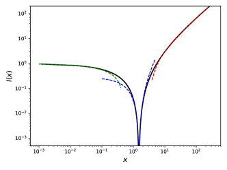
Figure 1: The rate function $I(x)$ for a two step process (eqs. 22,23) with $\alpha_{1}=\alpha_{2}=0.5$. Solid line : numerical Legendre transform of $\lambda(k)$ (eq. 25) ; dashed lines : approximate expressions given by eqs (26-28).

III.4 Extension to multi-component systems.

The dPGF$k$ method naturally generalizes to multi-component systems. As an example, consider the simplest (berg1978amodel, ; paulsson2005modelsof, ) chemical reaction modeling the production of mRNA and its encoded protein :

$$W(n,p\rightarrow n+1,p) = N$$

$$W(n,p\rightarrow n-1,p) = n$$

$$W(n,p\rightarrow n,p+1) = \alpha n$$

$$W(n,p\rightarrow n,p-1) = \beta p$$

where $(n,p)$ is the number of mRNA and proteins, $N$ the production rate of mRNA, $\alpha,\beta$ the production and degradation rate of proteins. Following the same arguments as above, the dPGFk equation is

$$\frac{\partial\phi}{\partial t} = N(z_{1}-1)\phi+a(z_{1},z_{2})\frac{\partial\phi}{\partial z_{1}}+b(z_{1},z_{2})\frac{\partial\phi}{\partial z_{2}}$$ (29)

where $z_{1},z_{2}$ are the conjugate variables to $n,p$,

$$a(z_{1},z_{2}) = (1-z_{1})+\alpha z_{1}(z_{2}-1)+k_{1}z_{1}$$ (30)

$$b(z_{1},z_{2}) = \beta(1-z_{2})+k_{2}z_{2}$$ (31)

and $k_{1},k_{2}$ are the amplitude of the tilted operator. Relation (29) is a linear first order PDE and can be solved exactly ; as we are only interested in the rates, we can look as before for vanishing points of the derivatives

$$a(z_{1}^{*},z_{2}^{*})=b(z_{1}^{*},z_{2}^{*})=0$$

that is

$$z_{2}^{*} = \frac{\beta}{\beta-k_{2}}$$

$$z_{1}^{*} = \frac{1}{1-k_{1}-\alpha(z_{2}^{*}-1)}$$

and therefore

$$\lambda(k_{1},k_{2})=N(z_{1}^{*}-1)=\frac{k_{1}+\alpha(z_{2}^{*}-1)}{1-k_{1}-\alpha(z_{2}^{*}-1)}$$

Taking the Legendre transform $I(\mathbf{x})=\sup_{\mathbf{k}}\left\{\mathbf{k.x}-\lambda(\mathbf{k})\right\}$, we find

$$I(x_{1},x_{2})=\left(\sqrt{N}-\sqrt{x_{1}}\right)^{2}+\left(\sqrt{\alpha x_{1}}-\sqrt{\beta x_{2}}\right)^{2}$$

We could have expected this result, as the transition rates for protein production has the same form that those for mRNA production, where $N$ has been replaced by $\alpha n$ : mRNA drives protein production but in this simple scheme, its own production is independent of the protein level.

III.5 Numerical computation.

The dPGF$k$ method is well suited to compute numerically $\lambda(k)$. As time flows, the solution of the dPGFk $\phi(z,t)$ converges to $\phi_{0}(z)\exp\left(\lambda(k)t\right)$. The dPGF$k$ equation is first order in time. Therefore, we can implement a discrete numerical scheme on a finite suitable interval $[L_{0},L_{1}]$: noting $dz,dt$ the discretization steps in in $z$ and $t$, $z_{i}=L_{0}+idz$ and $t_{j}=jdt$, one can compute $\phi(z_{i},t_{j+1})$ from $\phi(z_{i},t_{j})$. At a chosen point $z_{\alpha}$, at each time step $t_{j}$, the ratio $r_{j}=\phi(z_{\alpha},t_{j+1})/\phi(z_{\alpha},t_{j})$ is computed and $\phi(z_{i},t_{j+1})$ is normalized by this ratio:

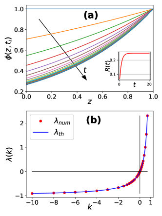
Figure 2: Numerical computation of $\lambda(k)$ of equation (13) with $N=1$ and initial condition $\phi(z,0)=1$. (a) For $k=0.25$, evolution of $\phi(z,t)$ as a function of $z$ for 50 times $t_{i}\in[0,20]$. At each time steps, $\phi(z,t+dt)$ is renormalized according to relation (32). Arrow indicates the direction of time. Inset : $R(t)=\log\left(\phi(1,t+dt)/\phi(1,t)\right)/dt$ as a function of time. (b)Numerical computation of $\lambda(k)$ as a function of $k$ (circles) and compared to its theoretical value given by expression (14).

$$\phi(z_{i},t_{j+1})\leftarrow\phi(z_{i},t_{j+1})/r_{j}$$ (32)

With this normalization, $\phi(z_{i},t_{j})\rightarrow\phi_{0}(z_{i})$, while

$$R_{j}=\frac{\log\left(r_{j}\right)}{dt}\rightarrow\lambda(k)$$

This algorithm, which is similar in its principle to the Lanczos algorithm(golub1996matrixcomputations, ), is illustrated in figure 2 for the case of the simple chemical reaction (equation 13) discussed in subsection III.1.

III.6 Discussions and conclusion.

The application of the dPGF$k$ method we have presented in this article was restricted to the cases where the transition rates $W(n\rightarrow n+m)$ were linear in the state of the system $n$. These systems give rise to first order PDE for $\phi(z,t;k)$ and therefore are exactly soluble. Moreover, as we are only interested in the long time behavior of the function $\phi()$, we usually even do not need to solve the PDE but can restrict the analysis to some particular points $z^{*}$ where the long time limit can be obtained through an ordinary differential equation.

Many interesting stochastic processes are quadratic in $n$ (see for example (nemoto2014finitesize, ; zilber2019agiant, ) where dynamical phase transition are observed ). The dPGF$k$ method for these cases leads to parabolic PDEs for $\phi()$ . The investigation of these equations is beyond the scope of this article as there is no general solution for them and they need to be investigated one a case by case basis. These equations however are of Schrodinger type and many more or less sophisticated methods are devoted in the literature to their investigations.

Higher order rate transitions give rise to PDEs that are less studied in the literature and therefore the dPGF$k$ method does not seem to be very useful for their investigation, even though the numerical method we have presented in subsection III.5 can still be used to obtain useful numerical results about their behavior. On the other hand, for transition rates that are not polynomial in the state $n$, the dPGF$k$ method of this article seems to be of limited use.

More complicated quantities than the time-average, such as $\bar{f}=(1/T)\int_{0}^{T}f\left(n(t)\right)dt$ can also be considered with the dPGF$k$ method, with the same limitations as discussed above. The diagonal matrix of DV in this case is ${\cal D}_{m}^{n}=\delta_{m}^{n}f(n)$ (touchette2018introduction, ); if $f(n)=n^{2}$, the dPGF$k$ method will contain a seconder order derivative of the form $z^{2}\partial^{2}\phi/\partial z^{2}$ and the resulting equation is still parabolic. Higher order terms, as discussed above, would be more difficult to investigate.

To summarize, in this paper, we have proposed a method (dPGF$k$) to compute the rate function $I(x)$ by embedding the tilted matrix of Donsker-Varadhan procedure into a partial differential equation, obtaining its largest eigenvalue $\lambda(k)$ through the long time analysis of the resulting equation and finding $I(x)$ by a Legendre transform of $\lambda(k)$. We believe that this method can constitute a useful tool in the analysis of large deviation of time-averaged stochastic processes.

Appendix A The dPGF$k$ equation.

The algebra for deriving the dPGF$k$ equation from the rate transitions is straightforward. Defining the PGF as

$$\phi(z,t)=\sum_{n}z^{n}P(n,t)$$

we have

$$\partial_{t}\phi = \sum_{n}z^{n}\partial_{t}P(n,t)$$

$$\partial_{z}\phi = \sum_{n}nz^{n-1}P(n,t)$$

$$\partial_{zz}\phi = \sum_{n}n(n-1)z^{n-2}P(n,t)$$

and so forth. Therefore, in the general dPGF$k$ equation :

$$\frac{\partial\phi(z,t)}{\partial t} = (z-1)\left\langle z^{n}W^{+}(n)\right\rangle+(1/z-1)\left\langle z^{n}W^{-}(n)\right\rangle$$ (33)

$$+ kz\frac{\partial\phi}{\partial z}$$

a term such as $\left\langle az^{n}\right\rangle$ where $a$ is a constant transforms into $\phi$, while a term such as $\left\langle nz^{n}\right\rangle$ transforms into $z\partial_{z}\phi$ etc.

For example, for $W^{+}(n)=N$ and $W^{-}(n)=n$ give rise to the equation

$$\partial_{t}\phi=N(z-1)\phi+(1/z-1)z\partial_{z}\phi+kz\partial_{z}\phi$$

which is equation (13) of subsection III.1.

For $W^{+}(n)=N-n$, $W^{-}(n)=n$ of subsection III.2, we have

$$\partial_{t}\phi=(z-1)\left(N\phi-z\partial_{z}\phi\right)+(1/z-1)z\partial_{z}\phi+kz\partial_{z}\phi$$

which is equation (III.2).

For multi-step processes with rates $W(n\rightarrow n+m)$, the dPGF$k$ equation is generally written as

$$\partial_{t}\phi=\sum_{m}(z^{m}-1)\left\langle z^{n}W(n\rightarrow n+m)\right\rangle+kz\partial_{z}\phi$$

the rules for transforming $\left\langle...\right\rangle$ into derivatives of $\phi$ being the same.

Appendix B General expression of the rate function for linear jump rates

It has been mentioned in the discussions above that when the transition rates $W(n\rightarrow n\pm 1)$ are first order polynomials of $n$, then the rate function is

$$I(x)=\left(W^{+}(x)-W^{-}(x)\right)^{2}$$

We demonstrate this statement here.

Consider a one-step stochastic process

$$W^{+}(n)=a+bn\,\,\,;\,\,\,W^{-}(n)=c+dn$$

the PGF$k$ associated to this process is

$$\frac{\partial\phi}{\partial t}=\left(bz^{2}-(b+d-k)z+d\right)\frac{\partial\phi}{\partial z}+\left(az+\frac{c}{z}-a-c\right)\phi$$

Let us first consider the case $b=0$. The prefactor of $\partial_{z}\phi$ vanishes at

$$z^{*}=\frac{d}{d-k}$$

and therefore

$$\lambda(k)=az^{*}+\frac{c}{z^{*}}-a-c$$ (34)

As $dz^{*}/dk=z^{*2}/d$, we have

$$x=\frac{d\lambda}{dk}=(az^{*2}-c)/d$$

reversing this relation, we have

$$z^{*2}=\frac{dx+c}{a}=\frac{W^{-}(x)}{W^{+}(x)}$$

As $k=d(1-1/z^{*})$, the rates read:

$$I(x) = kx-\lambda=a(z^{*}-1)^{2}$$ (35)

$$= \left(\sqrt{W^{+}(x)}-\sqrt{W^{-}(x)}\right)^{2}$$

Consider now the case $b\neq 0$ ; without loss of generality, we set $b=1$. The prefactor vanishes for the roots $z_{\pm}$ of the second order equation

$$z^{2}-(1+d-k)z+d=0$$

$\lambda(k)$ is still given by equation (34) and

$$x=\frac{d\lambda}{dk}=\frac{-az_{+}+cz_{-}/d}{z_{+}-z_{-}}$$

it is straightforward to show that, as before, $z_{+}^{2}=W^{-}(x)/W^{+}(x)$ and $z_{-}=d/z_{+}$. As $k=1+d-z_{+}-z_{-}$, after some algebraic manipulation, we find

$$I(x) = kx-\lambda$$

$$= W^{+}(x)+W^{-}(x)\pm 2\sqrt{W^{+}(x)W^{-}(x)}$$

As the rates $W$ are positive, we must choose the minus sign to have $I(x^{*})=0$ where $x^{*}$is such that $W^{+}(x^{*})=W^{-}(x^{*})$.

Appendix C Numerical computations.

The algorithm used for numerical computation of the largest eigenvalue discussed in subsection III.5 is an explicit finite difference scheme written in C where the function $\phi$ is discretized in space over $M=200$ points, $dz=\Delta L/M$ and $dt=0.5dz$. The algorithm for computing the discrete Legendre transform follows directly the definition (5) and has been written in Julia language (bezanson2017juliaa, ).

Acknowledgments.

We are grateful to Eric Bertin and Vivien Lecomte for detailed reading of the manuscript and fruitful discussions.

References

- [1] N. G. Van Kampen. Stochastic Processes in Physics and Chemistry. North Holland, Amsterdam ; Boston, 3 edition, 2007.
- [2] C Gardiner. Handbook of Stochastic Methods: for Physics, Chemistry and the Natural Sciences. Springer, 2004.
- [3] Hugo Touchette. The large deviation approach to statistical mechanics. Physics Reports, 478(1):1–69, July 2009.
- [4] Hugo Touchette. Introduction to dynamical large deviations of Markov processes. Physica A: Statistical Mechanics and its Applications, 504:5–19, August 2018.
- [5] M. D. Donsker and S. R. S. Varadhan. Asymptotic evaluation of certain markov process expectations for large time, I. Communications on Pure and Applied Mathematics, 28(1):1–47, 1975.
- [6] B Houchmandzadeh and M Vallade. Alternative to the diffusion equation in population genetics. Phys Rev E Stat Nonlin Soft Matter Phys, 82(5 Pt 1):51913, 2010.
- [7] Johan Paulsson. Models of stochastic gene expression. Physics of Life Reviews, 2(2):157–175, June 2005.
- [8] Pini Zilber, Naftali R. Smith, and Baruch Meerson. A giant disparity and a dynamical phase transition in large deviations of the time-averaged size of stochastic populations. Physical Review E, 99(5):052105, May 2019. arXiv: 1901.09384.
- [9] Baruch Meerson and Pini Zilber. Large deviations of a long-time average in the Ehrenfest urn model. Journal of Statistical Mechanics: Theory and Experiment, 2018(5):053202, May 2018.
- [10] Ido Golding, Johan Paulsson, Scott M. Zawilski, and Edward C. Cox. Real-Time Kinetics of Gene Activity in Individual Bacteria. Cell, 123(6):1025–1036, December 2005.
- [11] B. Houchmandzadeh, E. Dumonteil, A. Mazzolo, and A. Zoia. Neutron fluctuations: The importance of being delayed. Physical Review E, 92(5):052114, November 2015.
- [12] Otto G. Berg. A model for the statistical fluctuations of protein numbers in a microbial population. Journal of Theoretical Biology, 71(4):587–603, April 1978.
- [13] Golub. Matrix Computations 3e. Johns Hopkins University Press, Baltimore, 3rd revised edition edition, October 1996.
- [14] Takahiro Nemoto, Vivien Lecomte, Shin-ichi Sasa, and Frédéric van Wijland. Finite-size effects in a mean-field kinetically constrained model: dynamical glassiness and quantum criticality. Journal of Statistical Mechanics: Theory and Experiment, 2014(10):P10001, October 2014.
- [15] J. Bezanson, A. Edelman, S. Karpinski, and V. Shah. Julia: A Fresh Approach to Numerical Computing. SIAM Review, 59(1):65–98, January 2017.