Figure 1. Given a single scenery image, our method predicts the motion (e.g., moving clouds) and appearance (e.g., time-varying colors) separately to generate a cyclic animation via self-supervised learning of time-lapse videos using our convolutional neural networks that infer backward flow fields (insets) and color transfer functions for converting the input image. The flow fields are visualized using the colormap shown in Figures 8 and 9. The output frame size is $1,024\times 576$. Please see the supplemental video for the resultant animations. Input photo: Pixabay/Pexel.com.

Animating Landscape: Self-Supervised Learning of Decoupled Motion and Appearance for Single-Image Video Synthesis

Abstract.

Automatic generation of a high-quality video from a single image remains a challenging task despite the recent advances in deep generative models. This paper proposes a method that can create a high-resolution, long-term animation using convolutional neural networks (CNNs) from a single landscape image where we mainly focus on skies and waters. Our key observation is that the motion (e.g., moving clouds) and appearance (e.g., time-varying colors in the sky) in natural scenes have different time scales. We thus learn them separately and predict them with decoupled control while handling future uncertainty in both predictions by introducing latent codes. Unlike previous methods that infer output frames directly, our CNNs predict spatially-smooth intermediate data, i.e., for motion, flow fields for warping, and for appearance, color transfer maps, via self-supervised learning, i.e., without explicitly-provided ground truth. These intermediate data are applied not to each previous output frame, but to the input image only once for each output frame. This design is crucial to alleviate error accumulation in long-term predictions, which is the essential problem in previous recurrent approaches. The output frames can be looped like cinemagraph, and also be controlled directly by specifying latent codes or indirectly via visual annotations. We demonstrate the effectiveness of our method through comparisons with the state-of-the-arts on video prediction as well as appearance manipulation. Resultant videos, codes, and datasets will be available at http://www.cgg.cs.tsukuba.ac.jp/~endo/projects/AnimatingLandscape.

1. Introduction

From a scenery image, humans can imagine how the clouds move and the sky color changes as time goes by. Reproducing such transitions in scenery images is a common subject of not only artistic contents called cinemagraph [Bai et al., 2012; Liao et al., 2013; Oh et al., 2017] but also various techniques for image manipulation (e.g., scene completion [Hays and Efros, 2007], time-lapse mining [Martin-Brualla et al., 2015], attribute editing [Shih et al., 2013; Laffont et al., 2014], and sky replacement [Tsai et al., 2016]). However, creating a natural animation from a scenery image remains a challenging task in the fields of computer graphics and computer vision.

Previous methods in this topic can be grouped into two categories. The first category is the example-based approach that can create a realistic animation by transferring exemplars, e.g., fluid motion [Okabe et al., 2009; Prashnani et al., 2017] or time-varying scene appearance [Shih et al., 2013]. This approach, however, heavily relies on reference videos that match the target scene. The other category is the learning-based approach, which is typified by the recent remarkable techniques using Deep Neural Networks (DNNs).

DNN-based techniques have achieved great success in image generation tasks, particularly thanks to Generative Adversarial Networks (GANs) [Karras et al., 2018; Wang et al., 2018a] and other generative models, e.g., Variational Auto-Encoders (VAEs), which were also used to generate a video [Xiong et al., 2018; Li et al., 2018] from a single image. Unfortunately, the resolution and quality of the resulting videos are far lower than those generated in image generation tasks. One reason for the poor results is that the spatiotemporal domain of videos is too large for generative models to learn, compared to the domain of images. Another reason is the uncertainty in future frame predictions; for example, imagine clouds in the sky in a single still image. The clouds might move left, right, forward, or backward in the next frames according to the environmental factors such as wind. Due to such uncertainty, learning a unique output from a single input (i.e., one-to-one mapping) is intractable and unstable. The recent work using VAEs to handle the uncertainty is still insufficient for generating realistic and diverse results [Li et al., 2018].

In this paper, we propose a learning-based approach that can create a high-resolution video from a single outdoor image using DNNs. This is accomplished by self-supervised learning with a training dataset of time-lapse videos. Our key idea is to learn the motion (e.g., moving clouds in the sky and ripples on a lake) and the appearance (e.g., time-varying colors in daytime, sunset, and night) separately, by considering their spatiotemporal differences. For example, clouds move rapidly on the scale of seconds, whereas sky color changes slowly on the scale of tens of minutes, as shown in the riverside scene of Figure 1. Moreover, the moving clouds exhibit detailed patterns, whereas the sky color varies overall smoothly.

With this observation in mind, we learn/predict the motion and appearance separately using two types of DNN models (Figure 2) as follows. For motion, because one-shot prediction of complicated motion is difficult, our motion predictor learns the differences between two successive frames as a backward flow field. Long-term prediction is achieved by inputting the predicted frames recurrently. Motion-added images are then generated at high resolution by reconstructing pixels from the input image after tracing back the flow fields. For appearance, our predictor learns the differences between the input frame and arbitrary frames in each training video as spatially-smooth color transfer functions. In the prediction phase, color transfer functions are predicted at sparse frames and are applied to the motion-predicted frames via temporal interpolation. We assume that the motion and color variations in landscape time-lapse videos are spatiotemporally-smooth, and enforce such regularization in our training, which works well particularly with the motions of clouds in the sky and waves on water surfaces as well as the color variations of dusk/sunset in the sky. The output animation can be looped, inspired by cinemagraph.

To combat the uncertainty of future prediction, we also extract latent codes both for motion and appearance, which depict potential future variations and enable the learning of one-to-many mappings. The user can manipulate the latent codes to control the motion and appearance smoothly in the latent space. Note that the backward flow fields, color transfer functions, and latent codes are learned in a self-supervised manner because their ground-truth data are not available in general. Unlike previous techniques using 3D convolutions [Vondrick et al., 2016; Xiong et al., 2018; Li et al., 2018] for predictions with fixed numbers of frames, our networks adopt 2D convolutional layers. This approach allows fast learning and prediction and abolishes the limit on the number of predicted frames by recurrent feeding.

Our main contributions are summarized as follows:

• A framework for automatic synthesis of animation from a single outdoor image with fully convolutional neural network (CNN) models for motion and appearance prediction,

• Higher-resolution and longer-term movie generation by training with only hundreds to thousands of time-lapse videos in a self-supervised manner, and

• Decoupled control mechanism for the variations of motion and appearance that change at different time intervals based on latent codes.

We demonstrate these advantages by comparing with various methods of video prediction as well as attribute transfer. Our user study reveals that our results are subjectively evaluated as competitive or superior to those of previous methods or commercial software (see Appendix D). We also show applications for controlling the motion and appearance of output frames.

2. Related Work

Here we briefly review the related work of our technical components; optical flow prediction, color transfer, style transfer, video prediction, and so forth.

2.1. Optical Flow Prediction

Optical flow prediction from a single image has been studied with various approaches. Supervised approaches using CNNs have also been proposed [Walker et al., 2015; Gao et al., 2017]. The point is how to prepare ground-truth flow fields for supervised learning. The above-mentioned methods exploited existing techniques (e.g., FlowNet [Dosovitskiy et al., 2015], DeepFlow [Weinzaepfel et al., 2013; Revaud et al., 2016], and SpyNet [Ranjan and Black, 2017]) for generating ground-truth flow fields synthetically. However, we confirmed that previous methods relying on such synthetic data yield poor predictions for time-lapsed videos (see Section 6.2) for which no genuine ground-truth is available.

Recently, self-supervised approaches have been proposed for estimating flow fields between two input images [Ren et al., 2017; Wang et al., 2018b]. We also adopt a self-supervised approach where a flow field is computed between two consecutive frames. The main difference against the existing approaches is that we input only a single image in the inference phase and handle the prediction uncertainty by introducing latent codes.

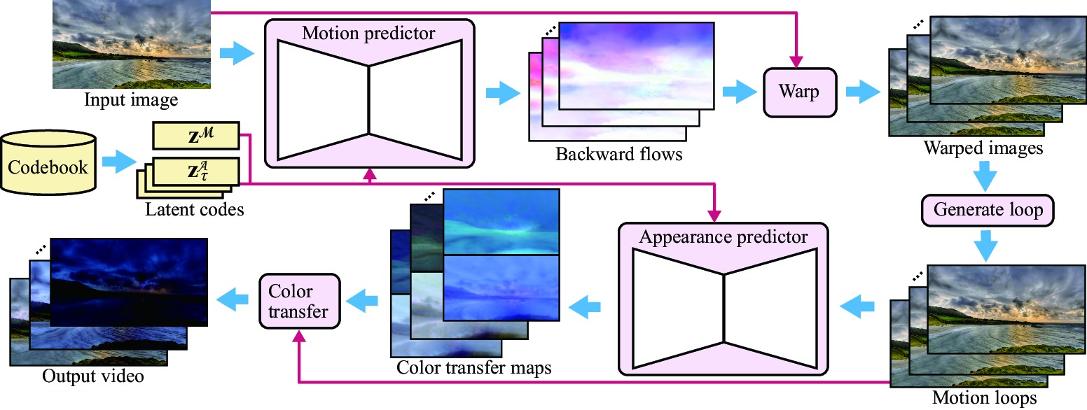
Figure 2. Overview of our inference pipeline. Given the input image and latent codes that control future variations, the motion predictor generates future backward flows. The flows are used to warp the input image to synthesize motion-added images, which are then converted to a cyclic motion loop. The appearance predictor generates color transfer maps, which are finally used for color transfer to obtain the output video. Input photo: Per Erik Sviland (Vvuxdqn-0vo)/Youtube.com.

2.2. Appearance Manipulation

Color transfer [Reinhard et al., 2001] is a fundamental technique for changing color appearance. This technique makes the overall color of a target image conform to that of a reference image while retaining the scene structure of the target, by matching the statistics (i.e., the mean and standard deviation) of the two images. The original method [Reinhard et al., 2001] is enhanced by respecting local color distributions using soft clustering [Tai et al., 2005] or semantic region correspondence [Wu et al., 2013]. There is also a color tone transfer method specialized in sky replacement [Tsai et al., 2016].

Style transfer can convey richer information, including textures using DNNs, than color transfer. The original work [Gatys et al., 2016] in this literature optimizes an output image via backpropagation of the perceptual loss for retaining the source content and style loss for transferring the target style. Faster transfer is accomplished by pre-training autoencoders for specific styles [Johnson et al., 2016] and using whitening and coloring transforms (WCTs) for arbitrary styles [Li et al., 2017]. Semantic region correspondence can also be integrated [Luan et al., 2017]. However, the strong expression power of style transfer works negatively for our purpose; it yields unnatural results for various scenes due to overfitting (see Section 6). We instead delegate the texture transfer to our motion predictor and change the color appearance using the transfer functions that can avoid overfitting.

A recent arXiv paper [Karacan et al., 2018] presents a method to manipulate attributes of natural scenes (e.g., night, sunset, and winter) via style transfer [Luan et al., 2017] and image synthesis using a conditional GAN. From a semantic layout of the input image and a target attribute vector, the method first synthesizes an intermediate style image, which is then used for style transfer with the input image. Animations can be generated by gradually changing the attribute vector, but enforcing temporal coherence is difficult with this two-step synthesis. In contrast, our method offers smooth appearance transitions via latent-space interpolation, as we demonstrate in Section 6.

2.3. Video Generation from a Still Image

An early attempt to animate a natural scene in a single image was a procedural approach called stochastic motion texture [Chuang et al., 2005]. This approach generates simple quasi-periodic motions of individual components, such as swaying trees, rippling water, and bobbing boats, with parameter tuning for each component.

Example-based approaches can reproduce realistic motion or appearance without complex parameters by directly transferring reference videos [Okabe et al., 2009, 2011, 2018; Prashnani et al., 2017; Shih et al., 2013]. However, their results become unnatural without an appropriate reference video similar to the input image. This issue can be alleviated at the cost of larger database and larger computational resource. Also, existing techniques often impose tedious manual processes for specifying, e.g., alpha mattes, flow fields and regions for fluid. Our method can generate high-resolution videos using only hundreds of megabytes of pre-trained data within a few minutes on a single GPU. Our method can run automatically yet can also be controlled using latent codes.

Example-based appearance transfer [Shih et al., 2013] can reproduce the time-varying color variations in a static image with a reference video. However, simple frame-by-frame transfer suffers from flickering artifacts for dynamic objects in the scene. Key-frame interpolation alleviates such flickering, which is not directly applicable if the outputs are videos containing dynamic objects, unlike ours. The method by Laffont et al. [2014] achieves appearance transfer using a manually-annotated database whereas our training datasets do not require manual annotations.

The past few years have witnessed the dramatic advances in learning-based approaches, particularly using DNN. For example, DNN architectures used for video prediction include not only 2DCNN [Xue et al., 2016; Mathieu et al., 2016; Lotter et al., 2017; Babaeizadeh et al., 2018; Hao et al., 2018] but also convolutional Recurrent Neural Networks (cRNNs) [Ranzato et al., 2014], Long Short-Term Memory (LSTM) [Srivastava et al., 2015; Zhou and Berg, 2016; Denton and Birodkar, 2017; Byeon et al., 2018], and 3DCNNs [Vondrick et al., 2016; Xiong et al., 2018; Li et al., 2018]. However, even with the state-of-the-art techniques [Xiong et al., 2018; Li et al., 2018], the frame length and resolution of generated videos are quite limited (i.e., up to 16 or 32 frames at $128\times 128$) due to the training complexity and architecture design. In a sharp contrast, our method can generate much higher-resolution videos with an unlimited number of frames by leveraging intermediate flow fields and color transfer functions, as we discuss in Section 6. Note that a recent work by Li et al. [2018] also predicts flow fields like our method. The key differences of our method are that i) their method requires ground-truth flow fields, whereas ours does not (i.e., learning is self-supervised); ii) their method uses 3DCNN, whereas ours uses 2DCNN, which reduces the training complexity; and iii) their method cannot provide direct control over appearance transition, whereas ours can because we employ decoupled training of motion and appearance.

3. Method Overview

Figure 2 shows the whole pipeline of our video synthesis, where our method first generates motion-added frames from the single input image, optionally makes them looped by linear blending, and then applies color transfer to each frame. As we explained in Section 1, our motion predictor infers backward flows recurrently, whereas our appearance predictor infers a color transfer function for each frame. This design is crucial for handling the well-known problem in recurrent inference where error accumulates in the cycled output frames [Shi et al., 2015]; in our motion prediction, error accumulates in the backward flows, which we assume are spatially-smooth and thus less sensitive to error. Each predicted frame is reconstructed by tracing back to the input image to avoid error accumulation in RGB values due to repetitive color sampling. In our appearance prediction, on the other hand, we avoid recurrent feeding and infer time-varying color transfer maps from the input image directly. Blur artifacts and error accumulation in output RGB values can be avoided because the per-pixel RGB value in the input image is sampled only once for each output frame in both predictions.

We handle the future uncertainty in both predictions using latent codes extracted in the training phases. By assuming that the overall motion throughout an animation sequence is similar, we control the motion in a single animation only with a single latent code. On the other hand, because our appearance predictor is trained with frame pairs between an input image and arbitrary frames in each training video, we require a latent code to control the appearance of each frame. Consequently, for appearance control of an animation sequence, we require a sequence of latent codes, which has the same length as the output frame length. The latent codes can be specified automatically or manually, from latent codes stored during training (hereafter we refer to them as a codebook).

4. Models

Hereafter, we describe our network models and distinguish the notations between motion and appearance with the superscripts $\mathcal{M}$ and $\mathcal{A}$, respectively. Our motion predictor $P^{\mathcal{M}}$ and appearance predictor $P^{\mathcal{A}}$ are encoder-decoders with the same architecture of a fully CNN. The inputs of the predictors are i) a linearly-normalized RGB image $\textbf{I}\in[-1,1]^{w\times h\times 3}$ (where $w$ and $h$ are image width and height) and ii) a latent code z to account for uncertainty of future prediction. Code $\textbf{z}^{\mathcal{M}}$ controls the motion in a whole sequence, whereas $\textbf{z}^{\mathcal{A}}$ controls the appearance of only a single frame. The outputs of the predictors are multi-channel intermediate maps that are then used to convert the input image I into an output RGB frame $\hat{\textbf{O}}\in[-1,1]^{w\times h\times 3}$, where we use a circumflex ( $\hat{}$ ) to indicate an inferred output.

In the following subsections, for motion and appearance, we first explain the inference phase to illustrate the use cases of the predictors and then describe how to train the networks.

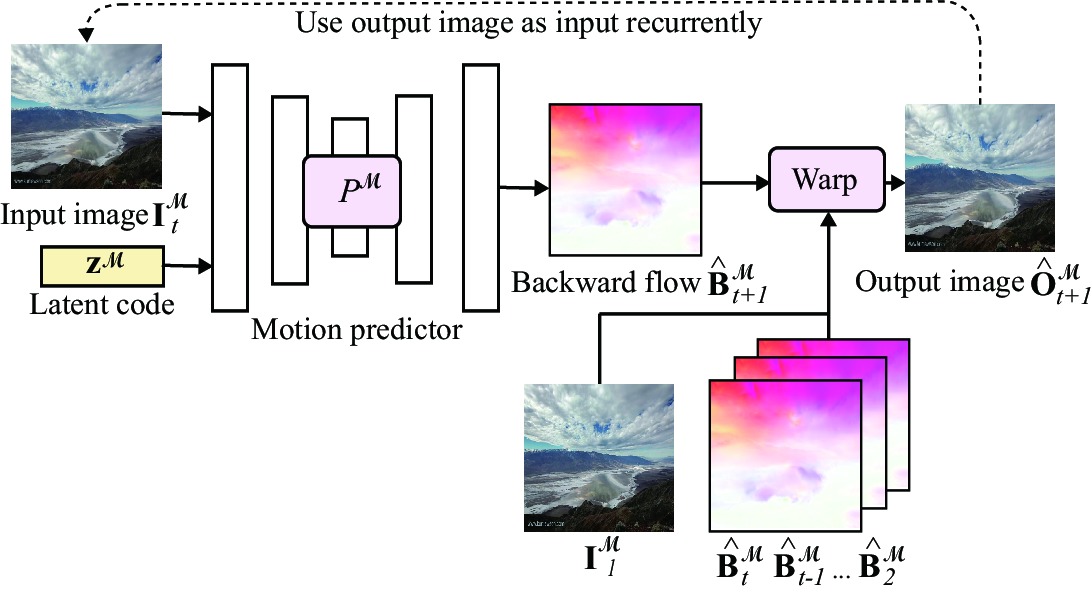
Figure 3. Recurrent inference using the motion predictor $P^{\mathcal{M}}$. A backward flow $\hat{\textbf{B}}_{t+1}^{\mathcal{M}}$ at time $t+1$ is predicted from an image $\textbf{I}_{t}^{\mathcal{M}}$ at time $t$ and a latent code $\textbf{z}^{\mathcal{M}}$. An output frame $\hat{\textbf{O}}_{t+1}^{\mathcal{M}}$ is obtained by warping $\textbf{I}_{t}^{\mathcal{M}}$ using $\hat{\textbf{B}}_{t+1}^{\mathcal{M}}$. $\hat{\textbf{O}}_{t+1}^{\mathcal{M}}$ is then used as the next input $\textbf{I}_{t+1}^{\mathcal{M}}$. This procedure is repeated to obtain multiple frames. Input photo: echoesLA (zleuiAR2syI)/Youtube.com.

4.1. Motion Predictor

Inference.

Given an input image $\mathbf{I}_{t=1}^{\mathcal{M}}$ ($=\mathbf{I}$, where $t$ indicates the time, i.e., the frame number) and a latent code $\textbf{z}^{\mathcal{M}}$, the motion predictor $P^{\mathcal{M}}$ infers a backward flow field $\hat{\textbf{B}}_{t+1}^{\mathcal{M}}\in[-1,1]^{w\times h\times 2}$ using $tanh$ for normalization. Here the pixel positions of $\textbf{I}^{\mathcal{M}}_{t}$ are normalized as $[-1,1]^{2}$. The pixel value at position $\mathbf{p}$ in the output frame $\hat{\textbf{O}}_{t+1}^{\mathcal{M}}$ is then reconstructed by sampling that in the current frame $\mathbf{I}_{t}^{\mathcal{M}}$ at $\mathbf{p}+\hat{\textbf{B}}_{t+1}^{\mathcal{M}}(\mathbf{p})$ via bilinear interpolation, where $\hat{\mathbf{B}}_{t+1}^{\mathcal{M}}(\mathbf{p})$ is the flow vector at $\mathbf{p}$. We call this reconstruction operation as warping in this paper. We recurrently use the predicted frames $\hat{\textbf{O}}_{t+1}^{\mathcal{M}}$ as the next motion predictor input $\textbf{I}_{t+1}^{\mathcal{M}}$(see Figure 3). However, if we warp the current frame to synthesize the next frame naïvely, the output frames will become gradually blurry, as explained in Section 3. Therefore, we instead warp flow fields $\hat{\mathbf{B}}_{t=2}^{\mathcal{M}}$, $\hat{\mathbf{B}}_{t=3}^{\mathcal{M}}$, $\dots$, $\hat{\mathbf{B}}_{t+1}^{\mathcal{M}}$ sequentially to accumulate flow vectors so that we can reconstruct each output frame $\hat{\textbf{O}}_{t+1}^{\mathcal{M}}$ from the input image $\mathbf{I}_{t=1}^{\mathcal{M}}$ directly.

Predicting flow fields in our self-supervised setting is challenging because it is essentially to find correspondences between two consecutive frames with large degrees of freedom, which is easily trapped into local optima yielding inconsistent flow fields. We thus restrict the range of the output flow fields both in prediction and training phases by assuming that the objects do not move significantly in a single timestep. Specifically, we divide inferred flow fields by a constant $\beta>1$ to restrict the range of their magnitudes to $[-1/\beta,1/\beta]^{2}$. Figure 4 demonstrates the effectiveness of $\beta$, with the results obtained after training only using the single image shown at the top left. Without this restriction (i.e., $\beta=1$), the estimated flow fields are inconsistent and the reconstructed images are corrupted. With this restriction (e.g., $\beta=64$), the reconstructed frames match to the ground-truth more closely, thanks to the consistent flow field estimation.

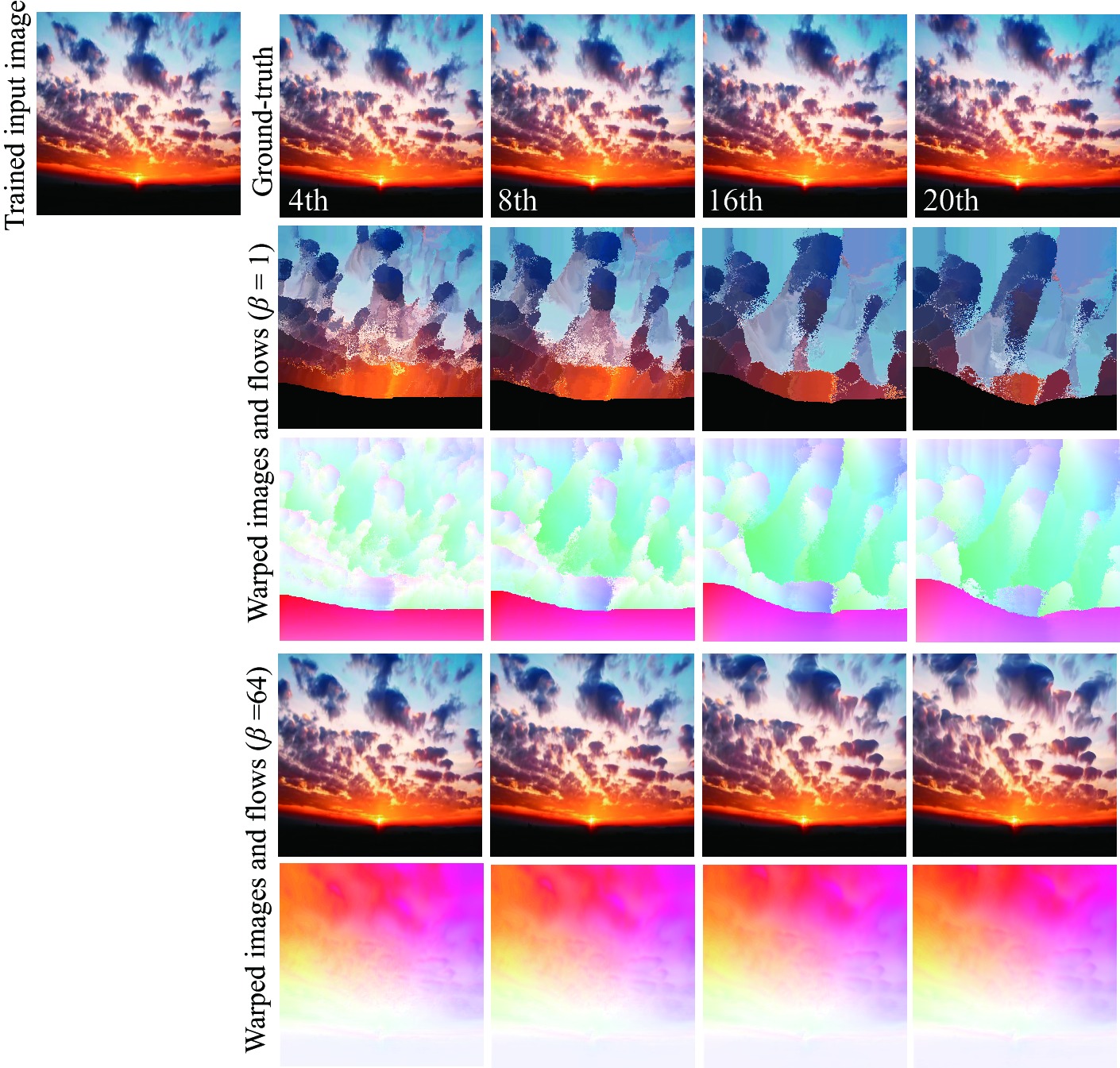
Figure 4. Motion restriction with constant $\beta$. The inferred flows become inconsistent without restriction (i.e., $\beta=1$) but yield warped images close to ground-truth frames with restriction (i.e., $\beta=64$). Input photos: Melania Anghel (rM7aPu9WV2Q)/Youtube.com.

Training.

A straightforward way for training the motion predictor is to minimize the difference between inferred and ground-truth flow fields, as done in [Walker et al., 2015; Gao et al., 2017; Li et al., 2018]. Our motion predictor, in contrast, learns future flow fields in a self-supervised manner only from time-lapse videos that have no ground-truth.

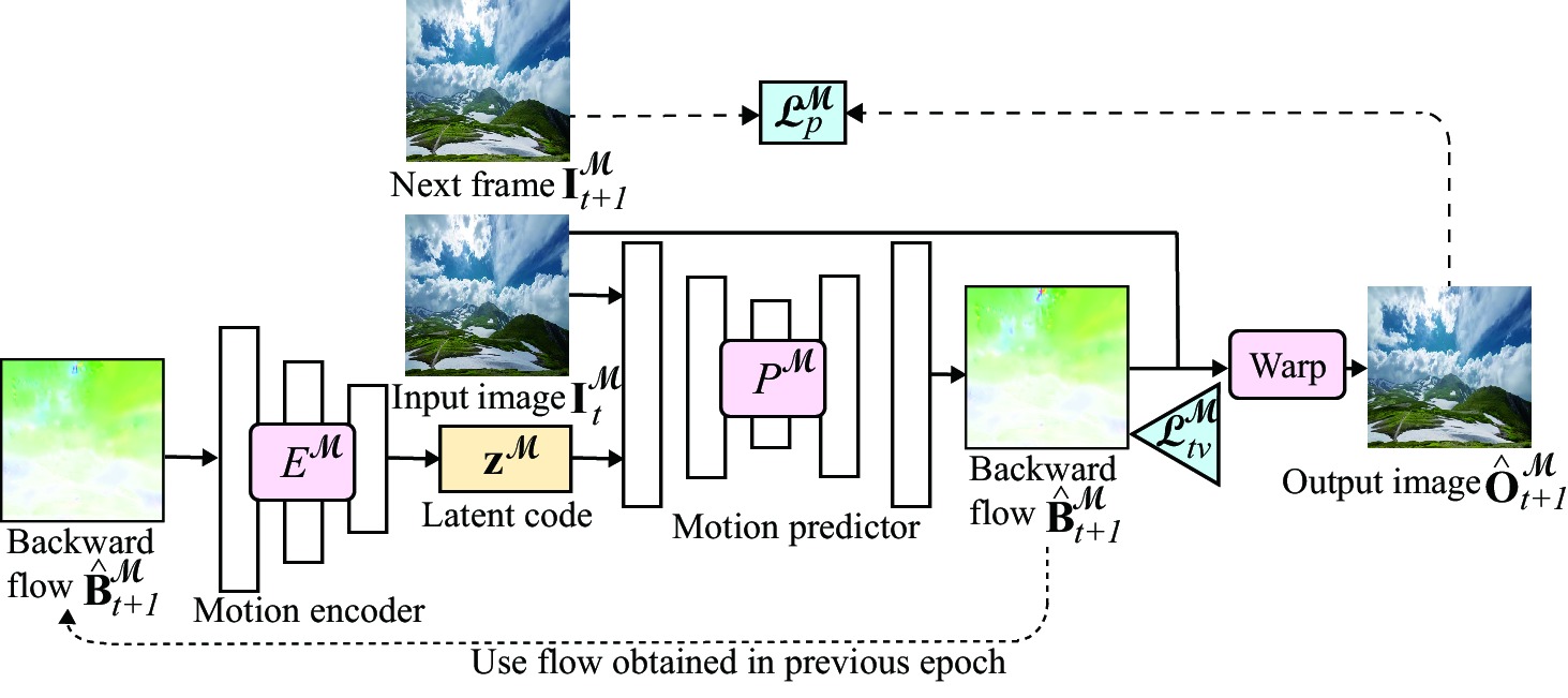
Figure 5. Training of the motion predictor $P^{\mathcal{M}}$. The training is done using consecutive frames $\textbf{I}^{\mathcal{M}}_{t}$ and $\textbf{I}^{\mathcal{M}}_{t+1}$ such that the loss $\mathcal{L}^{\mathcal{M}}_{p}$ between $\textbf{I}^{\mathcal{M}}_{t+1}$ and the output $\hat{\textbf{O}}^{\mathcal{M}}_{t+1}$ is minimized. $\hat{\textbf{O}}^{\mathcal{M}}_{t+1}$ is obtained by warping $\textbf{I}^{\mathcal{M}}_{t}$ using the backward flow $\hat{\textbf{B}}^{\mathcal{M}}_{t+1}$, which is regularized with the loss $\mathcal{L}^{\mathcal{M}}_{tv}$. $\textbf{z}^{\mathcal{M}}$ is obtained by encoding the previously inferred flow using the motion encoder $E^{\mathcal{M}}$ in our self-supervised setting where ground-truth flows do not exist. Input photos: Akio Terasawa (gRnKhf9Kw1Q)/Youtube.com.

Figure 5 outlines the training of the motion predictor. We first define a L2 loss for the network output $\hat{\textbf{O}}^{\mathcal{M}}_{t+1}$ obtained from the input image $\textbf{I}^{\mathcal{M}}_{t}$ and the next frame $\textbf{I}^{\mathcal{M}}_{t+1}$:

(1) $$\mathcal{L}^{\mathcal{M}}_{p}=\|\textbf{I}^{\mathcal{M}}_{t+1}-\hat{\textbf{O}}^{\mathcal{M}}_{t+1}\|_{2}^{2}\;,$$

where $\|\cdot\|_{2}$ means L2 norm. Also, a weighted total variation loss is applied to the output flow field for edge-preserving smoothing:

(2) $$\mathcal{L}^{\mathcal{M}}_{tv}=\displaystyle\sum_{\textbf{p},\textbf{q}\in N(\textbf{p})}w(\textbf{I}^{\mathcal{M}}_{t+1}(\textbf{p}),\textbf{I}^{\mathcal{M}}_{t+1}(\textbf{q}))\|\hat{\mathbf{B}}_{t+1}^{\mathcal{M}}(\textbf{p})-\hat{\mathbf{B}}_{t+1}^{\mathcal{M}}(\textbf{q})\|_{1},$$

(3) $$w(\textbf{x},\textbf{y})=\exp\left(-\frac{\|\textbf{x}-\textbf{y}\|_{1}}{\sigma}\right),$$

where $N(\textbf{p})$ indicates the right and above neighbors of p, and $\sigma$ is a constant to determine influence of this term. The output flow field $\hat{\mathbf{B}}^{\mathcal{M}}_{t+1}$ is smoothed using the weighting function $w$ such that $\hat{\mathbf{B}}^{\mathcal{M}}_{t+1}$ respects the color variations of the next frame $\mathbf{I}^{\mathcal{M}}_{t+1}$. Using weights $\lambda^{\mathcal{M}}_{p}$ and $\lambda^{\mathcal{M}}_{tv}$, our total training loss function is defined by

(4) $$\mathcal{L}^{\mathcal{M}}=\lambda^{\mathcal{M}}_{p}~{}\mathcal{L}^{\mathcal{M}}_{p}+\lambda^{\mathcal{M}}_{tv}~{}\mathcal{L}^{\mathcal{M}}_{tv}\;.$$

To handle future uncertainty and extract latent codes $\mathbf{z}^{\mathcal{M}}$, we simultaneously train the motion encoder $E^{\mathcal{M}}$. Problems similar to this one-to-many mapping were tackled in BicycleGAN [Zhu et al., 2017], where latent codes are learned from ground-truth images. In our case, the latent codes $\mathbf{z}^{\mathcal{M}}$ should be learned from the flow fields $\mathbf{B}^{\mathcal{M}}_{t+1}$, whose ground-truth are not available.

To overcome this chicken-and-egg problem, we initialize the input flow field of our motion encoder $E^{\mathcal{M}}$ as zero tensor in the first epoch, and gradually update it with $\textbf{B}^{\mathcal{M}}_{t+1}$ during the training phase. Another problem is that, because a pair of consecutive frames for training is selected randomly from each training video for each epoch (see Section 4.3), a naïve approach would initialize the input of $E^{\mathcal{M}}$ for each pair, which yields slow convergence. We thus re-use the input of $E^{\mathcal{M}}$ for each training video, assuming that frames throughout the video exhibit a similar motion. We refer to this re-used input as a common motion field for the training video and condition it on a single latent code $\mathbf{z}^{\mathcal{M}}$. A common motion field of each training video is stored in each epoch and used in the next epoch to extract the latent code $\mathbf{z}^{\mathcal{M}}$ of the corresponding video. In this way, we finally store the code $\mathbf{z}^{\mathcal{M}}$ in a codebook for the use in the inference phase. A pseudo-code of this training procedure is shown in Appendix A.2.

4.2. Appearance Predictor

Inference.

Given $\mathbf{I}^{\mathcal{A}}$ (equals a motion-added frame $\textbf{I}^{\mathcal{A}}_{t}$ at time $t$), our appearance predictor $P^{\mathcal{A}}$ infers a color transfer map $\hat{\textbf{C}}_{\tau}^{\mathcal{A}}=\{\hat{\mathbf{C}}_{\tau}^{w},\hat{\mathbf{C}}_{\tau}^{b}\}$ (where $\hat{\mathbf{C}}_{\tau}^{w},\hat{\mathbf{C}}_{\tau}^{b}\in[-1,1]^{w\times h\times 3}$) for an arbitrary frame $\tau$ (Figure 6). Each color transfer map $\hat{\textbf{C}}_{\tau}^{\mathcal{A}}$ is controlled by the latent code $z^{\mathcal{A}}_{\tau}$ at frame $\tau$. The output frame $\hat{\textbf{O}}_{\tau}^{\mathcal{A}}$ is then computed by applying the map $\hat{\textbf{C}}_{\tau}^{\mathcal{A}}$ to the input image $\mathbf{I}^{\mathcal{A}}$ as follows:

(5) $$\hat{\textbf{O}}_{\tau}^{\mathcal{A}} =\textsc{ColorTransfer}\left(\hat{\textbf{C}}_{\tau}^{\mathcal{A}},\textbf{I}^{\mathcal{A}}\right)$$

(6) $$=\tanh\left(\hat{\textbf{C}}_{\tau}^{w}\circ\textbf{I}^{\mathcal{A}}+\hat{\textbf{C}}_{\tau}^{b}\right),$$

where $\circ$ denotes Hadamard product and $tanh$ is used to restrict the pixel values of $\hat{\textbf{O}}_{\tau}^{\mathcal{A}}$ within $[-1,1]$.

In the final video generation (Section 5), we first interpolate the latent code sequence $\{\mathbf{z}_{\tau}^{\mathcal{A}}\}$ linearly, and then apply color transfer to each frame.

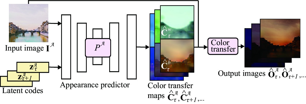
Figure 6. Inference using the appearance predictor $P^{\mathcal{A}}$. Color transfer maps $\hat{\textbf{C}}_{\tau}^{\mathcal{A}}=\{\hat{\textbf{C}}_{\tau}^{w},\hat{\textbf{C}}_{\tau}^{b}\}$ at time $\tau$ are computed from an input image $\textbf{I}^{\mathcal{A}}$ and latent code $\textbf{z}^{\mathcal{A}}_{\tau}$. An output frame $\hat{\textbf{O}}_{\tau}^{\mathcal{A}}$ is obtained by applying color transfer to $\textbf{I}^{\mathcal{A}}$. Multiple frames are obtained using latent code sequence $\{\textbf{z}^{\mathcal{A}}_{\tau}\}$, unlike the recurrent feeding used in the motion predictor $P^{\mathcal{M}}$. Input photo: Domenico Loia/Unsplash.com.

Training.

Figure 7 outlines the training of the appearance predictor. We first define loss functions between two frames with different appearances sampled from the training dataset. To learn style conversion for the entire image, we use a style loss between the inferred output frame $\hat{\textbf{O}}^{\mathcal{A}}_{\tau}$ and the ground-truth target frame $\textbf{I}^{\mathcal{A}}_{\tau}$:

(7) $$\mathcal{L}^{\mathcal{A}}_{s}=\displaystyle\sum_{l}\|G(F_{l}(\textbf{I}^{\mathcal{A}}_{\tau}))-G(F_{l}(\hat{\textbf{O}}^{\mathcal{A}}_{\tau}))\|_{2}^{2}\;,$$

where the function $F_{l}$ outputs feature maps obtained from the $l$-th layer of the pre-trained VGG16 [Simonyan and Zisserman, 2014]. The function $G$ outputs the Gram matrix of the features maps. Inspired by the existing style transfer algorithm [Johnson et al., 2016], we use relu_2_2, relu_3_3, and relu_4_3 as the layers $l$. Note that the style loss is insensitive to spatial color distributions due to the Gram matrix, which makes, for example, a partially red sky during sunset difficult to handle. Therefore, an additional weak constraint is imposed on the output frame $\hat{\textbf{O}}^{\mathcal{A}}_{\tau}$ to roughly conform to the spatial color distributions:

(8) $$\mathcal{L}^{\mathcal{A}}_{sp}=\|SP(\textbf{I}^{\mathcal{A}}_{\tau})-SP(\hat{\textbf{O}}^{\mathcal{A}}_{\tau})\|_{2}^{2}\;,$$

where $SP$ indicates the spatial pyramid pooling function [He et al., 2015], which outputs fixed-size feature maps by dividing an image into multi-level grids. We set the pyramid height as one and divide the image into a $32\times 32$ grid, where average pooling is applied to each cell. Whereas the above losses are defined against the ground-truth target frame $\textbf{I}^{\mathcal{A}}_{\tau}$, a content loss is defined against the input $\textbf{I}^{\mathcal{A}}$ to keep the input scene structure:

(9) $$\mathcal{L}^{\mathcal{A}}_{c}=\displaystyle\sum_{l}\|F_{l}(\mathbf{I}^{\mathcal{A}})-F_{l}(\hat{\textbf{O}}^{\mathcal{A}}_{\tau})\|_{2}^{2}\;.$$

As the layer $l$ in this loss function, we use relu_1_2 only to retain high-frequency components of the input scene. Finally, the inferred color transfer map $\hat{\textbf{C}}_{\tau}^{\mathcal{A}}$ is regularized to improve the generalization ability of the model:

(10) $$\mathcal{L}^{\mathcal{A}}_{tv}=\displaystyle\sum_{\textbf{p},\textbf{q}\in N(\textbf{p})}w(\textbf{I}^{\mathcal{A}}(\textbf{p}),\textbf{I}^{\mathcal{A}}(\textbf{q}))\|\hat{\mathbf{C}}^{\mathcal{A}}_{\tau}(\textbf{p})-\hat{\mathbf{C}}^{\mathcal{A}}_{\tau}(\textbf{q})\|_{1}.$$

Note that, unlike Equation (2), these color transfer maps are smoothed such that $\hat{\textbf{C}}_{\tau}^{\mathcal{A}}$ respects the scene structure of the input image $\textbf{I}^{\mathcal{A}}_{t}$. Total loss $\mathcal{L}^{\mathcal{A}}$ is then given by the summation of the above losses with weights $\lambda^{\mathcal{A}}_{s}$, $\lambda^{\mathcal{A}}_{sp}$, $\lambda^{\mathcal{A}}_{c}$, and $\lambda^{\mathcal{A}}_{tv}$:

(11) $$\mathcal{L}^{\mathcal{A}}=\lambda^{\mathcal{A}}_{s}~{}\mathcal{L}^{\mathcal{A}}_{s}+\lambda^{\mathcal{A}}_{sp}~{}\mathcal{L}^{\mathcal{A}}_{sp}+\lambda^{\mathcal{A}}_{c}~{}\mathcal{L}^{\mathcal{A}}_{c}+\lambda^{\mathcal{A}}_{tv}~{}\mathcal{L}^{\mathcal{A}}_{tv}\;.$$

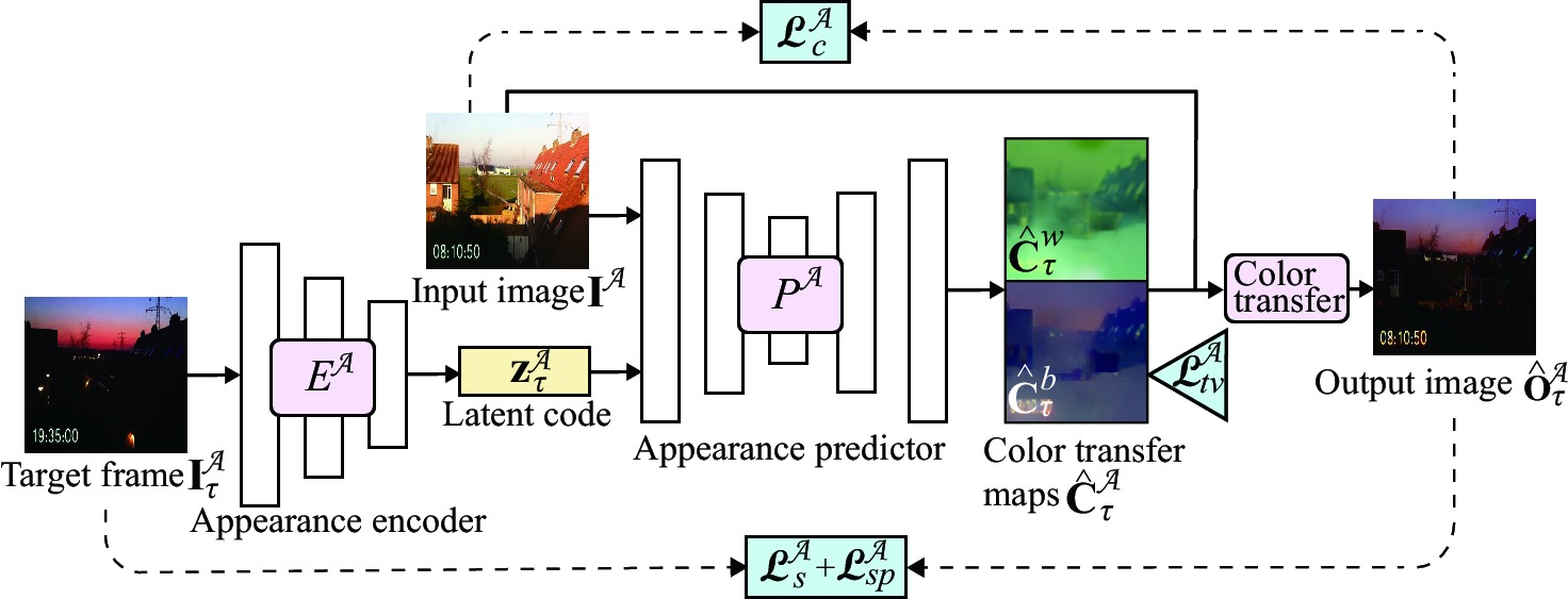
Figure 7. Training of the appearance predictor $P^{\mathcal{A}}$. The training uses each pair of a source image $\textbf{I}^{\mathcal{A}}$ and a target image $\textbf{I}^{\mathcal{A}}_{\tau}$ such that the losses $\mathcal{L}^{\mathcal{A}}_{s}$ and $\mathcal{L}^{\mathcal{A}}_{sp}$ between $\textbf{I}^{\mathcal{A}}_{\tau}$ and $\hat{\textbf{O}}^{\mathcal{A}}_{\tau}$ are minimized. $\hat{\textbf{O}}^{\mathcal{A}}_{\tau}$ is obtained via color transfer based on $\hat{\textbf{C}}^{\mathcal{A}}_{\tau}$ to $\textbf{I}^{\mathcal{A}}$. The losses $\mathcal{L}^{\mathcal{A}}_{c}$ and $\mathcal{L}^{\mathcal{A}}_{tv}$ impose that the content of $\textbf{I}^{\mathcal{A}}$ be preserved in $\hat{\textbf{O}}^{\mathcal{A}}_{\tau}$ and $\hat{\textbf{C}}^{\mathcal{A}}_{\tau}$ be regularized, respectively. $\textbf{z}^{\mathcal{A}}_{\tau}$ is obtained by encoding the target image $\textbf{O}^{\mathcal{A}}_{\tau}$ using the appearance encoder $E^{\mathcal{M}}$. Input photos: Anonymous (a8CTqQAxBzI)/Youtube.com.

We also train the appearance encoder $E^{\mathcal{A}}$ to extract latent codes $\textbf{z}^{\mathcal{A}}_{\tau}$ simultaneously using $\mathcal{L}^{\mathcal{A}}$. The input of the appearance encoder $E^{\mathcal{A}}$ is the target frame $\textbf{I}^{\mathcal{A}}_{\tau}$ so that the inferred output $\hat{\textbf{O}}_{\tau}^{\mathcal{A}}$ is conditioned on $\textbf{I}^{\mathcal{A}}_{\tau}$. After the training, a sequence of latent codes $\{\mathbf{z}^{\mathcal{A}}_{\tau}\}$ for each training video is extracted using $E^{\mathcal{A}}$ and stored in a codebook, similarly to the motion predictor.

4.3. Implementation

The network architectures of our predictors are summarized in Appendix A.1. The motion and appearance predictors $P^{\mathcal{M}}$ and $P^{\mathcal{A}}$ are fully CNNs, each of which consists of three downsampling layers, five residual blocks, and three upsampling layers. The networks contain skip connections also used in U-Net [Ronneberger et al., 2015]. Our motion and appearance encoders $E^{\mathcal{M}}$ and $E^{\mathcal{A}}$ adopt the same network structure as that in resnet_128 [Zhu et al., 2017], which consists of six layers for convolution, pooling, and linear transformation.

To avoid training biases by longer video clips, we train each pair of frames sampled randomly for each video clip in each epoch. Whereas the motion predictor $P^{\mathcal{M}}$ learns from a pair of consecutive frames, the appearance predictor $P^{\mathcal{A}}$ learns from any pair of frames. The pseudo-codes of the training procedures are described in Appendix A.2.

The training image size $w\times h$ was set to $256\times 256$ for the predictors and $128\times 128$ for the encoders for both motion and appearance. The number of dimensions of the latent codes z was set to 8. We used the Adam optimizer [Kingma and Ba, 2014] with a learning rate of $1.0\times 10^{-4}$, two coefficients of $\{0.5,0.999\}$, and a batch size of 8 for backpropagation. Regarding the weights of the loss functions, we empirically chose $\lambda^{\mathcal{M}}_{p}=1$, $\lambda^{\mathcal{M}}_{tv}=1$, $\lambda^{\mathcal{A}}_{s}=1$, $\lambda^{\mathcal{A}}_{sp}=1\times 10^{-2}$, $\lambda^{\mathcal{A}}_{c}=1\times 10^{-5}$, $\lambda^{\mathcal{A}}_{tv}=0.1$, and $\sigma=0.1$.

5. Single-image Video Generation

Now we explain how to generate a video from a single image by integrating the two predictors. Inspired by cinemagraph, the output animation can be looped as an option. Here we explain the looped version.

Algorithm 1 summarizes the procedure of our video generation. The motion prediction first generates a sequence of frames $\mathcal{V^{M}}$, which is then converted to a looped one $\mathcal{V}^{\mathcal{M}}_{loop}$. A sequence of output frames $\mathcal{V}$ are finally generated from $\mathcal{V}^{\mathcal{M}}_{loop}$ through the appearance prediction. Note that $\mathcal{V}^{\mathcal{M}}$ is used instead of $\mathcal{V}^{\mathcal{M}}_{loop}$ if the looping process is not required. To make a motion loop $\mathcal{V}^{\mathcal{M}}_{loop}$ from the non-periodic sequence $\mathcal{V^{M}}$, various methods can be used [Schödl et al., 2000; Liao et al., 2015]. Among the several methods that we tested, simple cross-fading  [Schödl et al., 2000] worked relatively well for making plausible animations without significant discontinuities. Whereas the resolutions of images $\mathbf{I}$, the output frames in $\mathcal{V^{M}}$, $\mathcal{V}^{\mathcal{M}}_{loop}$, and the final video $\mathcal{V}$ are not limited, the inputs to the predictors and encoders are resized to fixed resolutions for training. The inferred flow fields and color transfer maps are resized to the original size and then applied to the original input image. We do not magnify output frames directly to avoid blurring. To handle sampling outside of previous flow fields during the reconstruction of output frames, reflection padding is applied to the input image and previous flow fields.

Algorithm 1. Single-image Video Generation

Input: Input image I, latent codes $z^{\mathcal{M}}$, $\{z^{\mathcal{A}}_{\tau}\}$

Output: Output video $\mathcal{V}=\{\textbf{I}_{1},\textbf{I}_{2},...\}$

//Motion prediction

1: $\mathcal{V^{M}}\leftarrow\{\textbf{I}\}$

2: $\textbf{I}^{\mathcal{M}}_{t=1}\leftarrow\textbf{I}$

3: for each frame do

4:     $\hat{\textbf{B}}^{\mathcal{M}}_{t+1}\leftarrow$ Resize$(P^{\mathcal{M}}$(Resize$(\textbf{I}^{\mathcal{M}}_{t}),\textbf{z}^{\mathcal{M}}))$

5:     $\hat{\textbf{O}}^{\mathcal{M}}_{t+1}\leftarrow$ Warp($\{\hat{\textbf{B}}^{\mathcal{M}}_{t+1},\hat{\textbf{B}}^{\mathcal{M}}_{t},\ldots,\hat{\textbf{B}}^{\mathcal{M}}_{t=2}\},\textbf{I}^{\mathcal{M}}_{t=1})$

6:     $\mathcal{V^{M}}\leftarrow\mathcal{V^{M}}\bigcup\hat{\textbf{O}}^{\mathcal{M}}_{t+1}$

7:     $\textbf{I}^{\mathcal{M}}_{t+1}\leftarrow\hat{\textbf{O}}^{\mathcal{M}}_{t+1}$

8: endfor

9: $\mathcal{V}^{\mathcal{M}}_{loop}\leftarrow$ GenerateLoop($\mathcal{V^{M}}$)

//Appearance prediction

10: $\mathcal{V}\leftarrow\phi$

11: $\{\textbf{z}^{\mathcal{A}}_{t}\}\leftarrow$ InterpolateLatentCodes$(\{\textbf{z}^{\mathcal{A}}_{\tau}\})$

12: for all $\textbf{z}^{\mathcal{A}}_{t}$ in $\{\textbf{z}^{\mathcal{A}}_{t}\}$ do

13:     $\textbf{I}^{\mathcal{A}}\leftarrow$ GetNextFrameCyclically$(\mathcal{V}^{\mathcal{M}}_{loop})$

14:     $\hat{\textbf{C}}^{\mathcal{A}}_{t}\leftarrow P^{\mathcal{A}}($Resize$(\textbf{I}^{\mathcal{A}}),\textbf{z}^{\mathcal{A}}_{t})$

15:     $\hat{\textbf{O}}^{\mathcal{A}}_{t}\leftarrow$ ColorTransfer(Resize$(\hat{\textbf{C}}^{\mathcal{A}}_{t}$),$\textbf{I}^{\mathcal{A}})$

16:    $\mathcal{V}\leftarrow\mathcal{V}\bigcup\hat{\textbf{O}}^{\mathcal{A}}_{t}$

17: endfor

We can control the future variations of output frames with latent codes $z^{\mathcal{M}}$ and $\{z^{\mathcal{A}}_{\tau}\}$, and also adjust the speeds of motion and appearance. The latent codes can be selected randomly (in this case, automatically) or manually from the codebook. We also show some applications to control latent codes indirectly in Section 6.4. The motion speed can be adjusted by simply multiplying flow fields by an arbitrary scalar value. Meanwhile, the appearance speed is determined in two ways; by adjusting the number of latent codes in a sequence obtained from the codebook, or by repeating the motion loop $\mathcal{V}^{\mathcal{M}}_{loop}$ an integer number of times during one cycle of appearance variation. We adopt the latter for all the looped videos. The latent code sequence for appearance at key-frames are linearly interpolated to generate latent codes for the whole frames. We also interpolate the final and initial latent codes to generate a cycle.

6. Experiments

We implemented our system with PyTorch library running on a PC with NVIDIA GeForce GTX 1080 Ti GPUs. We stopped training after 5,000 epochs, and the computation time was about one week on a single GPU. Motion and appearance inferences to generate a $640\times 320$ frame took 0.054 seconds and 0.058 seconds, respectively. Overall computation time to generate a cinemagraph of 1,010 frames was 98 seconds, which included trained model parameter loadings to a GPU of 9 seconds, motion inference of 11 seconds, motion loop generation of 6 seconds, and appearance inference of 59 seconds. The other processes consumed the remaining time.

The results in our paper are demonstrated in the supplemental video. The directions and magnitudes of optical flow vectors are visualized using the pseudo colors shown in Figure 8.

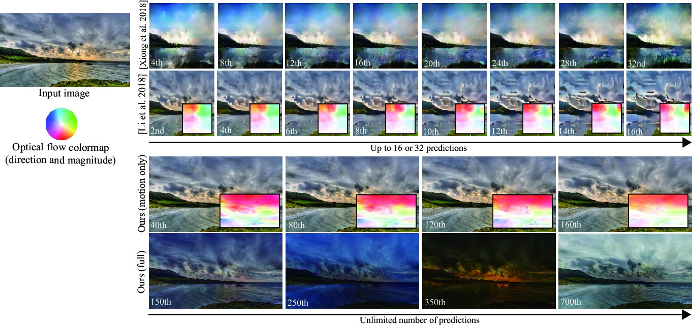
Figure 8. Qualitative comparison with the state-of-the-art video generation by Xiong et al. [2018] and Li et al. [2018]. Their and our output resolutions are $128\times 128$ and $640\times 360$, respectively. Input photo: Per Erik Sviland (Vvuxdqn-0vo)/Youtube.com.

6.1. Dataset Generation

For training the motion predictor and encoder, we used the time-lapse video dataset published by Xiong et al. [2018]. The dataset was divided into 1,825 video clips for training and 224 clips for testing at the resolution of $640\times 360$. To avoid learning motions that were too subtle, we first sampled every other frame from each training video clip and then automatically omitted pairs of frames in which the average of differences of pixel values of consecutive frames was less than 0.02. The resultant video clips contain 227 frames on average.

Because the videos used for motion modeling are too short to observe appearance transitions, we collected 125 one-day video clips from YouTube and the dataset published by Shih et al. [2013] for appearance modeling. Because appearance changes more slowly than motion, we omitted more redundant frames from the dataset. Specifically, we first sampled frames about every 10 minutes in real-world time for each video clip, and then omitted consecutive frames containing smaller appearance variations. To do this, we computed the sum of the RGB differences of the average of the pixel values for the consecutive frames, and adjacent frames were automatically omitted if the corresponding sum was less than 0.3. With this sampling process, the number of frames for each training clip is reduced to 15 on average. Note that the input images shown in this paper were not included in the training data unless otherwise noted.

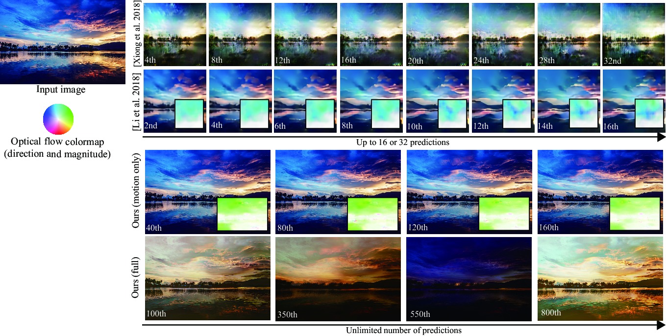
Figure 9. Another qualitative comparison with the state-of-the-art video generation by Xiong et al. [2018] and Li et al. [2018]. Their and our output resolutions are $128\times 128$ and $1024\times 683$, respectively. Input photo: Fancycrave.com/Pexels.com.

6.2. Comparisons with Video Prediction Models

To clarify the advantages of our method, we compared it with the state-of-the-art video prediction models for a single input image. The comparison models are 3DCNN encoder-decoders [Li et al., 2018] that predict flow fields for a fixed number frames from an input image and generate future frames based on the predicted flows. To train the comparison models, we used the same training data [Xiong et al., 2018] as ours, and ground-truth flow fields were created using SpyNet [Ranjan and Black, 2017] based on the authors’ codes [Li et al., 2018]. We used their default parameters and image size. The number of epochs was also the same as ours (5,000), and improvement was not observed with more epochs. We also compared our method with other recent GAN-based models [Xiong et al., 2018].

Figures 8 and 9 show qualitative comparisons. The right images are generated frames and flow fields using each method from the upper-left image. As shown by the insets in the second and third rows, our method generates more plausible flow fields than the previous method according to the input scene structure; for example, whereas the clouds and the water surface move differently, the lands remain static overall. In the first row, the GAN-based method severely suffers from artifacts even in low-resolution images. In the second row, the generated frames by Li et al. are unnaturally abstracted despite the model’s two-phase design that first predicts flow fields and then generates future frame pixels. Our results are clearer and higher-resolution as demonstrated in the third row. Moreover, our method can theoretically generate an unlimited number of frames. Finally, as shown in the third row, our method can generate a looped animation that also contains appearance variations, thanks to decoupled learning, whereas the comparative method cannot handle it sufficiently.

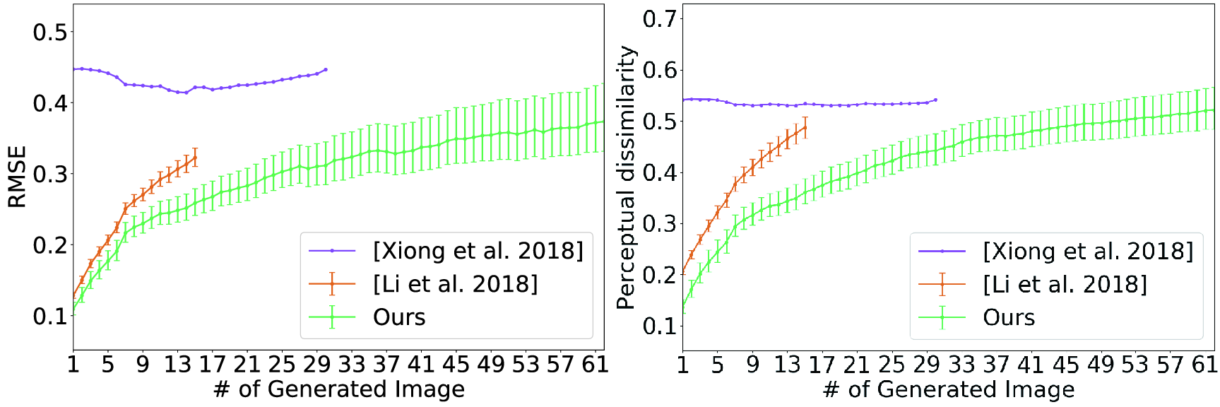
Figure 10. Quantitative comparisons with ground-truth for 224 test video clips. RMSE (left) and perceptual dissimilarity [Zhang et al., 2018] (right) are computed for each predicted frame. The solid lines and error bars denote average, minimum, and maximum values of the metrics, respectively.

In addition, we conducted quantitative evaluations using 224 test video clips with the methods by Xiong et al. [2018] and Li et al. [2018], regarding the accuracy compared to ground-truth successive frames. We compared differences between generated sequences and ground-truth ones frame-by-frame. As evaluation metrics, we used RMSE and perceptual dissimilarity [Zhang et al., 2018] based on Alex-Net [Krizhevsky et al., 2012]. Because our results depend on latent codes, we compared average, minimum, and maximum values of evaluation metrics for five latent codes sampled from the codebook. The previous method [Li et al., 2018] based on VAE can also synthesize different future sequences, and thus we sampled different noises five times from the normally distributed latent space for generating five sequences, which are used to calculate the metrics in the same manner as ours. Figure 10 shows the frame-by-frame RMSEs and perceptual dissimilarities for each method. The solid lines and error bars denote average, minimum, and maximum values of the metrics computed from the different future sequences. The increasing trends in both graphs imply that long-term prediction is challenging. Nevertheless, our method outperforms the state-of-the-art method in that ours can generate higher-resolution and longer sequences. In particular, our results are perceptually more similar to the ground-truth sequences, even when generated with different parameters.

6.3. Comparisons on Appearance Manipulation

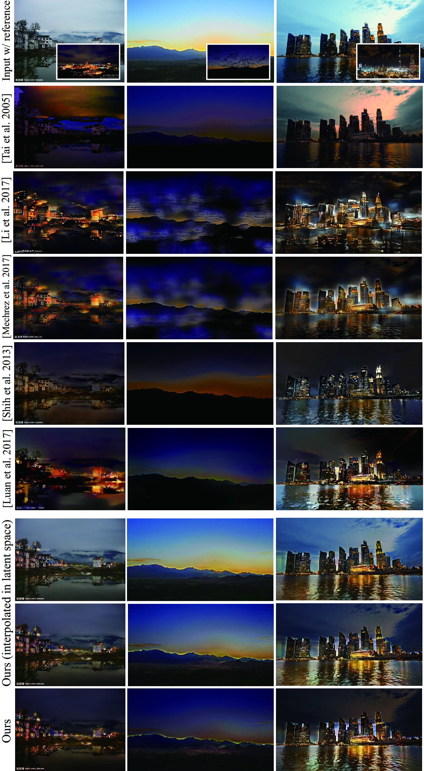
Figure 11. Comparisons with previous methods for appearance manipulation. From left to right, the output image sizes are $700\times 525$, $700\times 394$, and $700\times 394$, respectively. Input photos: Shih et al. [2013].

We further compared our appearance-only results with those of previous color/style transfer methods. Figure 11 shows the results of appearance transfer obtained using the source and target images (inset) in the top row. For the local color transfer [Tai et al., 2005] in the second row, the appearance variations are monotonic and inconsistent with the scene structures. Style transfer based on WCT [Li et al., 2017] in the third row can handle more diverse appearance variations but some artifacts can be observed. Although these artifacts are alleviated by solving the screened Poisson equation [Mechrez et al., 2017] as shown in the fourth row, the results are still unnatural. On the other hand, the example-based hallucination [Shih et al., 2013] (fifth row) and deep photo style transfer  [Luan et al., 2017] (sixth row) successfully transfer the target appearances. These methods, however, require a target video and an additional semantic segmentation map, respectively. Even worse, when applied to videos, frame-by-frame optimization will cause flickering artifacts, and key-frame interpolation cannot be used with dynamic objects. Our results in the bottom row are generated without any additional inputs, except for latent codes encoded from target images. Thanks to latent codes, natural and smooth interpolation is possible in the latent space, as demonstrated from the seventh to ninth rows where the appearance changes from the source to the target. Moreover, we can dispense even with target images if latent codes are specified from the codebook or are predicted from source images via LSTM prediction (see Appendix B).

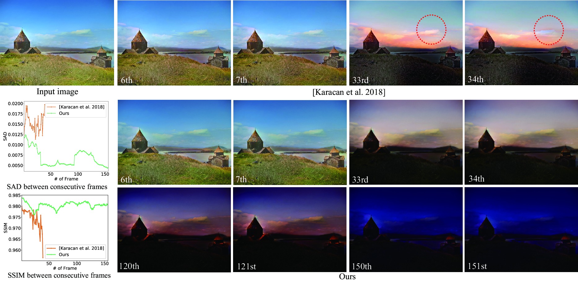
Figure 12. Comparisons with the state-of-the-art attribute manipulation by Karacan et al. [2018]. The red circles indicate flicker artifacts in their results. In contrast, our method can reproduce smoothly-varying appearances. We also tried to quantitatively visualize this difference based on the sum of absolute distance and structural similarity between consecutive frames. The output resolution is $640\times 480$. Input photo: Heretiq/Wikipedia.com.

Figure 13. Comparisons with commercial appearance editing software (Photoshop Match Color). The input image is the same as that in Figure 12, and the target images are also used to extract the latent codes for our method. The fade parameter (from 0 to 100) can control the degree of color transfer.

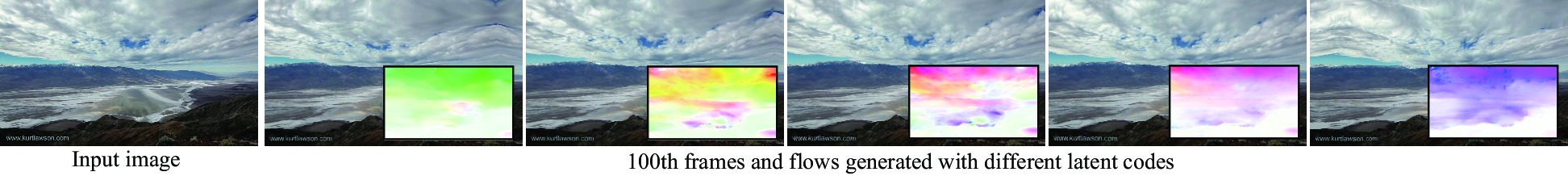
Figure 14. Effects of latent codes for motion. The input latent codes are extracted via self-supervised learning, and sorted along the first principle axis in the codebook. We can see that the output frames are also aligned according to the input latent codes. The output resolution is $640\times 360$. Input photo: echoesLA (zleuiAR2syI)/Youtube.com.

To the best of our knowledge, there are no methods using generative models for appearance variation, except for the recent one for manipulating image attributes [Karacan et al., 2018]. This method can be applied to generation of videos containing appearance transitions by gradually changing attributes. Therefore, in Figure 12, we compared our appearance predictor with their method using the input image and results on their project page. In our results, we selected the latent codes that yield appearances similar to those of the compared results. As demonstrated in the first row, for each output frame, the compared method can generate semantically plausible appearances that match the image content. Their sequence, however, contains flickering artifacts due to the two-stage synthesis where temporal consistency is difficult to impose as is. In the second and third rows, we can see that our result is free from noticeable artifacts. We can generate temporally-coherent animations thanks to keyframe interpolation in the latent space, unlike the compared method. Also, we tried to quantitatively visualize such artifacts by computing the sum of absolute differences and structural similarity between the consecutive frames, as shown at the lower left. The resultant values imply that our method allows smoother transition than the compared method. In addition, we compared commercial appearance editing software (Photoshop Match Color). Figure 13 demonstrates that local appearance transitions cannot be reproduced by the software, unlike our method. The halo artifacts behind the cottage roof in Figure 13 is stronger than ours in Figure 12. Note that, in the supplemental video, the resultant animation using the commercial software was generated by repeatedly applying color transfer to intermediate frames using multiple target images. In this case, the halo artifact is reduced unexpectedly, but the global color variation becomes monotonic due to error accumulation. Our method can avoid such error accumulation thanks to the latent-space interpolation.

6.4. Controlling Future Variations

6.4.1. Effects of latent codes.

To verify that our method can handle future uncertainty and can learn meaningful latent space in an unsupervised manner, i.e., without any ground-truth labels such as wind directions or time labels (e.g., “daytime” or “night”), we investigated how latent codes affect outputs. Figure 14 shows the examples of motion. Here we sorted latent codes in the codebook according to the first principle component and applied them to the same input image. As we can see from the optical flows, our method generates similar motions from similar latent codes, while retaining a wide variety of motions. For appearance, a sequence $\{\mathbf{z}^{\mathcal{A}}\}$ contains time-varying latent codes, and thus we can see that similar consecutive latent codes yield smooth transition in a time series (please check our supplemental video). Figure 15 also demonstrates that diverse appearances (e.g., sunset, twilight, and night) can be reproduced from the same input image with different latent code sequences.

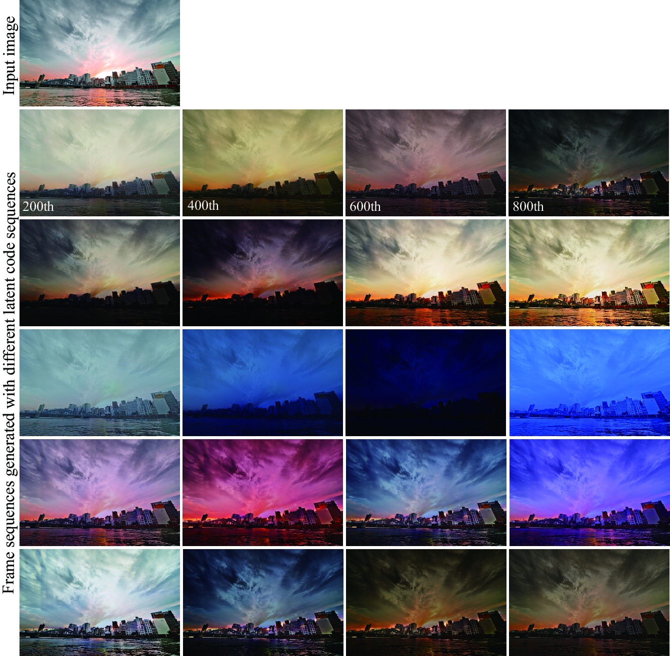
Figure 15. Effects of latent codes for appearance. In a frame sequence in each row, diverse appearances are synthesized from a different latent code sequence in the codebook. The output resolution is $700\times 466$. Input photo: Jezael Melgoza/Unsplash.com.

Whereas direct use of latent codes from the codebook yields natural transition (e.g., from daytime to sunset in appearance) because they are extracted from real time-lapse videos, we also provide means to indirectly specify latent codes, namely, using arrow annotations for motion and image patches for appearance, as explained below.

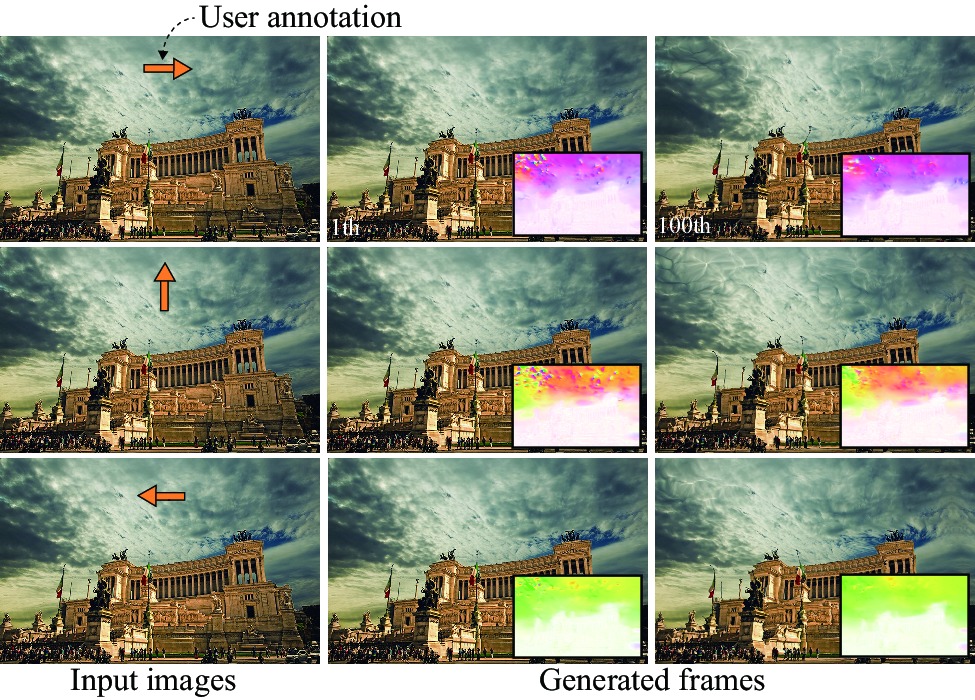
Figure 16. Motion specification using arrow annotations. The output resolution is $640\times 411$. Input photo: Pixabay/Pexels.com

6.4.2. Motion control using arrow annotations

We offer arrow annotations for specifying flow directions of motion, as shown in the left column in Figure 16. We represent these sparse annotations as 2D maps $\mathbf{U}^{\mathcal{M}}\in[-1,1]^{w\times h\times 2}$, where pixels corresponding to the arrows have the specified flow vectors. Given $\textbf{U}^{\mathcal{M}}$ and an input image $\textbf{I}^{\mathcal{M}}$, an optimum latent code $\hat{\textbf{z}}^{\mathcal{M}}$ is obtained via optimization w.r.t. $\mathbf{z}^{\mathcal{M}}$ while fixing the network parameters of the motion predictor $P^{\mathcal{M}}$, as done in [Gatys et al., 2016]:

(12) $$\hat{\textbf{z}}^{\mathcal{M}}=\mathop{\rm arg~{}min}\limits_{\textbf{z}^{\mathcal{M}}}\|\max(\textbf{0},\textbf{M}\circ(\textbf{1}-D(\textbf{U}^{\mathcal{M}},P^{\mathcal{M}}(\textbf{I}^{\mathcal{M}},\textbf{z}^{\mathcal{M}}))-\textbf{m}))\|_{2}^{2},$$

where the function $D$ gives a map containing the cosine of an angle between two flows for each pixel. The mask $\mathbf{M}\in\{0,1\}^{w\times h}$ is used to compute error on arrows only, and $\textbf{m}\in\mathbb{R}^{w\times h}$ is a constant margin map (having 0.5 for each pixel) that allows a certain level of difference between estimated flows and specified flows. We used the Adam optimizer [Kingma and Ba, 2014] for this optimization. Using $\hat{\textbf{z}}^{\mathcal{M}}$ and $\textbf{I}^{\mathcal{M}}$, we recurrently predict image sequences containing motions similar to the directions of the annotations. The middle and right columns in Figure 16 demonstrate that entire flow fields are plausibly generated using the sparse annotations. Optimization for each user edit took about seven seconds.

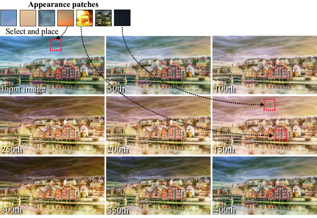
Figure 17. Appearance specification using image patches. The output resolution is $1,024\times 571$. Input photo: Pixabay/Pexels.com

6.4.3. Appearance control using image patches

We offer a means to specify the appearance at specific positions and frames using image patches. Using a map $\mathbf{U}^{\mathcal{A}}\in[-1,1]^{w\times h\times 3}$ containing information of placed patches, an optimum latent code $\hat{\textbf{z}}^{\mathcal{A}}$ is obtained, similarly to Equation (12):

(13) $$\hat{\textbf{z}}^{\mathcal{A}}\!\!=\mathop{\rm arg~{}min}\limits_{\textbf{z}^{\mathcal{A}}}\|\textbf{M}\circ(\textbf{U}^{\mathcal{A}}\!\!-\textsc{ColorTransfer}(P^{\mathcal{A}}(\textbf{I}^{\mathcal{A}}\!\!,\textbf{z}^{\mathcal{A}}),\textbf{I}^{\mathcal{A}})\|_{2}^{2}.$$

Figure 17 shows the results obtained via latent space interpolation between the input image and $\hat{\textbf{z}}^{\mathcal{A}}$. We can further change its appearance by placing multiple appearance patches as shown in the right image in the middle row. Cyclic animations can also be created via interpolation between the final and input images as demonstrated in the 300th to 400th frames.

6.5. Ablation Study

We conducted an ablation study to investigate the effectiveness of our loss functions. Figure 18 shows comparisons between the generated frames with and without each of the loss functions. Without the motion regularization term $\mathcal{L}^{\mathcal{M}}_{tv}$, the resultant flow fields in the third row are often inconsistent with the scene structure due to overfitting. For the same reason, the lack of the appearance regularization term $\mathcal{L}^{\mathcal{A}}_{tv}$ also causes noticeable artifacts (see our supplemental video) in the generated frames in the sixth row. Moreover, without the loss function $\mathcal{L}^{\mathcal{A}}_{sp}$ for learning spatial color distributions, the appearances vary uniformly, as shown in the fifth row, and the partially-reddish sky due to sunset is not sufficiently reproduced. In contrast, we can see that the resultant frames generated with the full losses in the second and fourth rows are more stable than the others.

Direct in Figure 18 means that the output images were inferred directly without color transfer functions. For this, we used a CNN with the same architecture as the appearance predictor except for the three-channel output. Although this CNN was trained with the full losses (the TV loss was applied to network outputs), the results are less natural than the others.

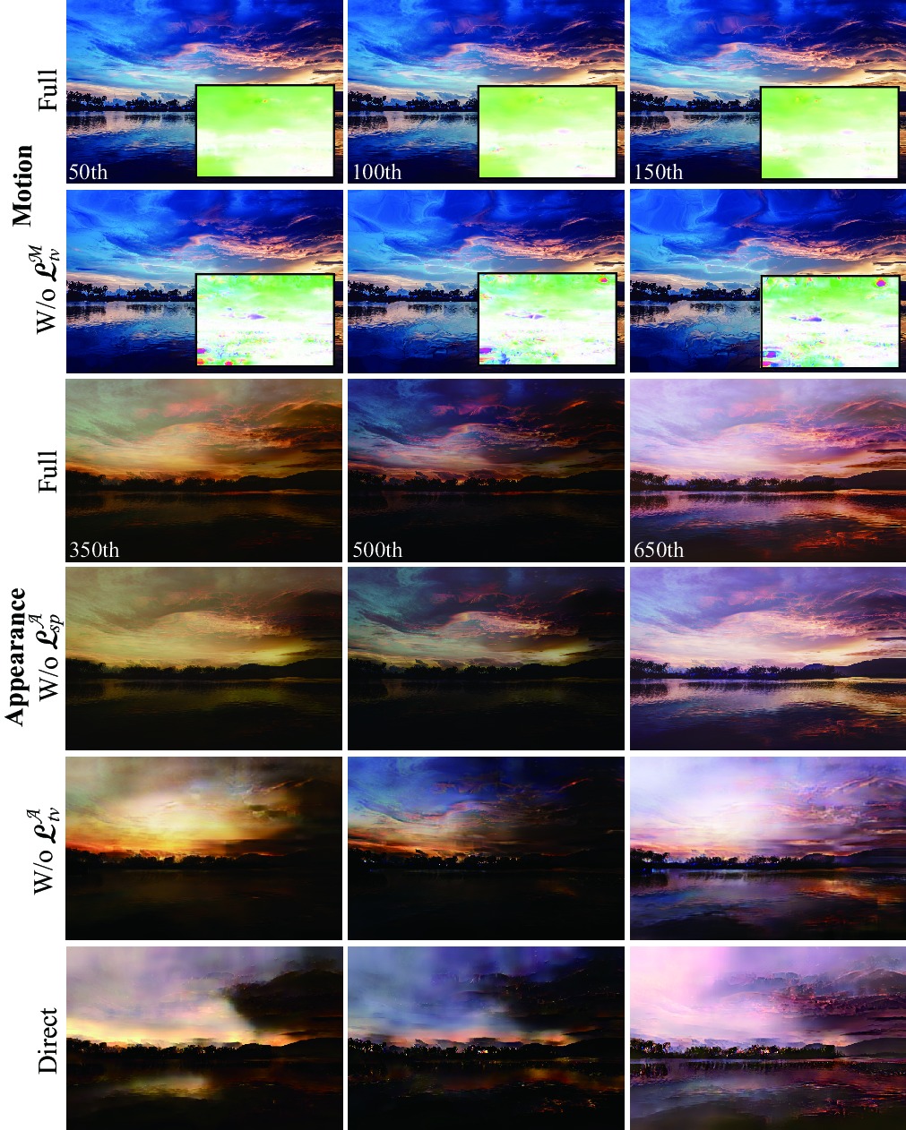
Figure 18. Ablation study of loss functions. The input image is the same as that in Figure 9. “Direct” means direct inference of output frames without color transfer. The output resolution is $1,024\times 683$.

6.6. Discussion

Do latent codes need regularization?

To make search of latent codes in a latent space more stable, there is an additional training option for adopting regularizers used by Variational Auto-Encoder (VAE) [Kingma and Welling, 2013] and Wasserstein Auto-Encoder (WAE) [Tolstikhin et al., 2017]. Whereas we regard the direct use of stored latent codes as the default choice because they yield plausible results, VAE and WAE allow us to select latent codes from regularized latent space, without referring to the codebook. In Figure 19, the predictors trained with these regularizers generated the results using latent codes sampled from a Gaussian distribution. In particular, the WAE regularizer is effective for generating more various outputs than the VAE regularizer because latent codes of different examples can stay far away from each other. In contrast, we can see that the models trained without these regularizers failed to generate plausible results from Gaussian latent codes. Although the regularization for training latent codes is not essential in our case because we use the codebook and how to select appropriate sequences of latent codes for appearance from regularized latent space is not clear without the codebook, it might be useful for future applications.

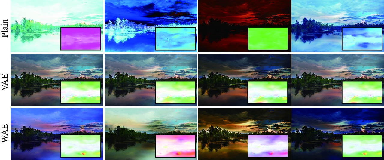
Figure 19. Comparison of with and without regularizations used in VAE and WAE. The appearance and motion (insets) in each column are inferred using the same latent code randomly sampled from a Gaussian distribution. The input image is the same as that in Figure 1.

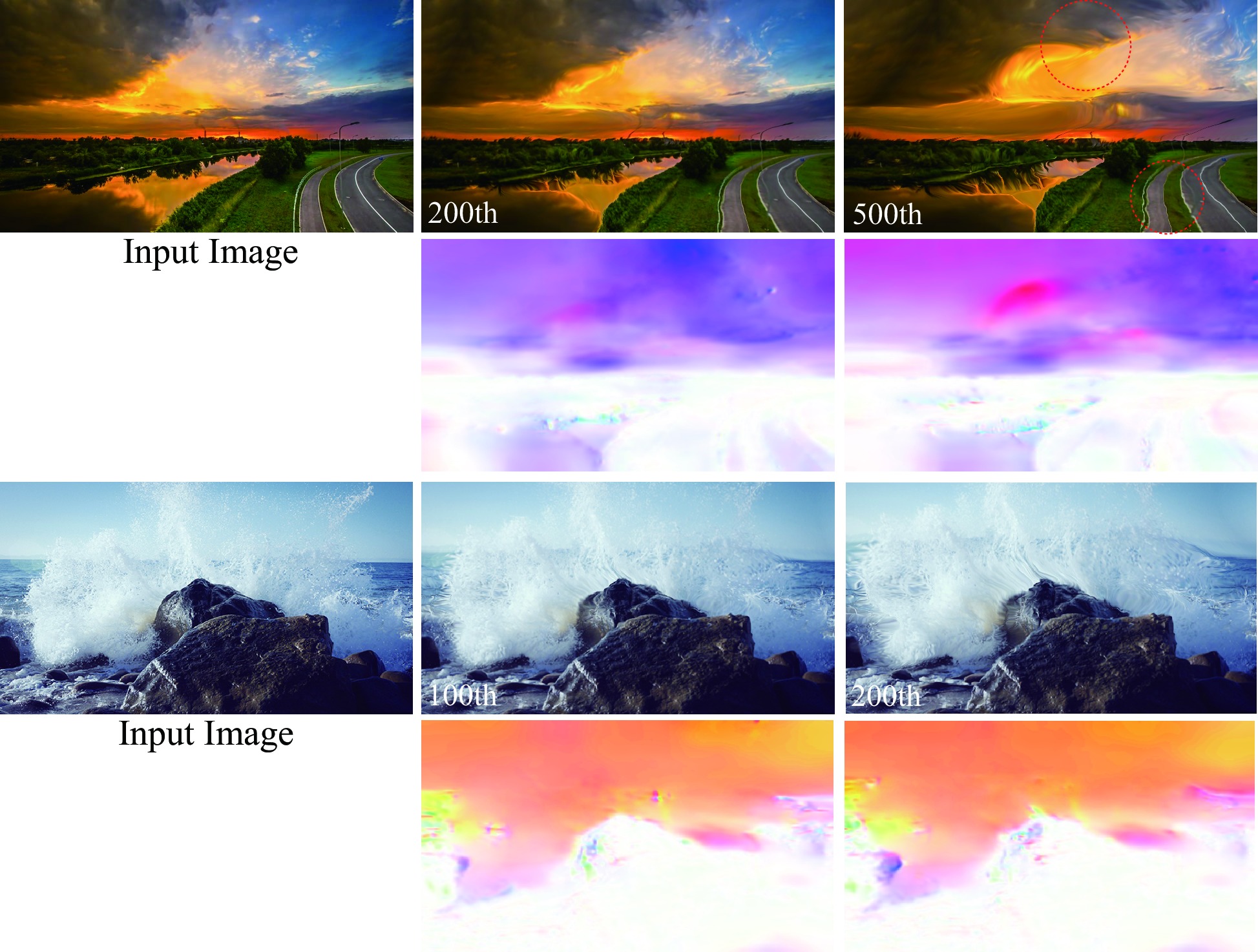
Figure 20. Failure cases. Very long-term prediction causes distortions (red circles in the top right), and non-uniform motions are difficult to reproduce (bottom rows). The output resolutions are $640\times 360$ (top) and $600\times 338$ (bottom), respectively. Input photos: Race The World (jZOLRAIUW2s)/Youtube.com and Justin Leibow/Unsplash.com.

Limitations

Although our motion predictor can generate an unlimited number of frames, very long-term prediction causes unnatural distortions because predicted frames are reconstructed only from an input image. The first row in Figure 20 shows an example, where the clouds in the 500th predicted frame are unnaturally stretched and the border of the road is deformed, compared to those in the 200th frame. Also, our method erroneously generates uni-directional motion even for objects that should exhibit scattered motions such as splashes, as shown in the third and fourth rows in Figure 20. There is still room for improvement in handling specific targets; cloud motions sometimes look unnatural, and mirror images of the sky on the water surface do not move synchronously in our results. When the user controls cloud motions (Section 6.4.2), the reflected motions on water surfaces are also changed but do not necessarily move consistently with the clouds. These artifacts might be alleviated by introducing specialized loss function(s) (e.g., physically- or geometrically-inspired loss functions for clouds and mirror images) and training data for each target.

There is also a trade-off between the diversity of output videos and the generalization ability of the models. To handle more various motions and appearances, a straightforward solution is to reduce the regularization weights while restricting unnatural deformations and artifacts to a tolerable level.

We mainly focus on landscape animations, especially of skies and waters, and put other types of animations where something appears (e.g., flower florescence or building construction) outside the scope. Nonetheless, we believe that our scope covers a wide variety of landscape videos and our motion predictor can also handle other types of motions (e.g., crowd motions seen from a distance) that can be well described with flow fields.

7. Conclusion

This paper has presented a method that can create a plausible animation at high resolution from a single scenery image. We demonstrated the effectiveness of our method by qualitatively and quantitatively comparing it with not only the state-of-the-art video prediction models but also other appearance manipulation methods. To the best of our knowledge, it is unprecedented to synthesize high-resolution videos with separated control over motion and appearance variations. This was accomplished by self-supervised, decoupled learning and latent-space interpolation. Our method can generate images with higher-resolution and longer-term sequences than previous methods. This advantage comes from the indirect image synthesis using intermediate maps predicted via training with regularization, rather than directly generating output frames as done in previous methods. The output sequences can also be controlled using latent codes extracted during training, which can be specified not only directly from the codebook but also indirectly via simple annotations.

One future direction is to improve the proposed model to create higher-quality animations. For example, additional information for semantic segmentation might be helpful for improving the performance, as done in existing style transfer methods [Luan et al., 2017]. Our current method does not adopt this approach to avoid the influence of segmentation error. Occlusion information [Wang et al., 2018b] could be incorporated explicitly into training of the motion predictor. We believe that our work has taken a significant step in single-image synthesis of videos and will inspire successive work for diverse animations.

Appendix A Implementation Details of Our DNNs

A.1. Network Architectures

Table 1. Network architecture of the motion predictor and appearance predictor. Concat(z) means concatenation between each pixel of input feature maps and z. For 2D convolutional layers and residual blocks, C is the number of channels, K is the kernel width and height, S is the stride, and P is the padding. Upsample(2) means magnifying input feature maps twice using nearest-neighbor interpolation.

Components	Layers	Specifications
	conv1	Concat(z), Conv2D(C(128), K(5), S(2), P(2)), LeakyReLU(0.1)
Downsampling	conv2	Concat(z), Conv2D(C(256), K(3), S(2), P(1)), InstanceNorm(256), LeakyReLU(0.1)
	conv3	Concat(z), Conv2D(C(512), K(3), S(2), P(1)), InstanceNorm(512), LeakyReLU(0.1)
Residual	res1, $\ldots$, res5	ResBlock2D(C(512), K(3), S(1), P(1))
	upconv1	Concat(conv3), Upsample(2), Conv2D(C(256), K(3), S(1), P(1)), InstanceNorm(256), LeakyReLU(0.1)
Upsampling	upconv2	Concat(conv2), Upsample(2), Conv2D(C(128), K(3), S(1), P(1)), InstanceNorm(128), LeakyReLU(0.1)
	upconv3	Concat(conv1), Upsample(2), Conv2D(C(3) or C(6), K(5), S(1), P(2))

Table 2. Network architecture of the motion encoder and the appearance encoder. Notations are the same as those in Table 1.

Component	Layers	Specifications
	conv1	Conv2D(C(64), K(4), S(2), P(1))
	res1	ResBlock2D(C(128), K(3), S(1), P(1))
Encoder	res2	ResBlock2D(C(192), K(3), S(1), P(1))
	res3	ResBlock2D(C(256), K(3), S(1), P(1))
	pooling	LeakyReLU(0.2), AvgPool2D(8,8)
	fc	Linear(8)

Table 1 summarizes the architecture of our motion and appearance predictors $P^{\mathcal{M}}$ and $P^{\mathcal{A}}$, whereas Table 2 shows the network architecture of our motion and appearance encoders $E^{\mathcal{M}}$ and $E^{\mathcal{A}}$.

A.2. Training Algorithms

The training procedures are summarized in Algorithms 1 and 2. The motion and appearance predictors $P^{\mathcal{M}}$ and $P^{\mathcal{A}}$ are trained using the time-lapse video datasets $\mathcal{D^{M}}$ and $\mathcal{D^{A}}$. These datasets contain $N$ video clips $\mathcal{S}_{i}~{}(i=1,...,N)$, each of which consists of $T_{i}$ images $\mathcal{S}_{i}=\{\textbf{I}^{i}_{1},\textbf{I}^{i}_{2},...,\textbf{I}^{i}_{T_{i}}\}$ in a time series. Note that, in the training of our motion predictor (Algorithm 1), each minibatch $\{\mathcal{B}\}$ uses frames only from a specific set of video clips $\{S_{j}\}$ randomly selected in each epoch, and a latent code is learned and saved for each training video.

Algorithm 2. Training of Motion Predictor

Input: $\mathcal{D^{M}}=\{\mathcal{S}_{1},\mathcal{S}_{2},...,\mathcal{S}_{N}\}$, $\mathcal{S}_{i}=\{\textbf{I}^{i}_{1},\textbf{I}^{i}_{2},...,\textbf{I}^{i}_{T_{i}}\}$

1: for $i=1$ to $N$ do

2:     Common motion field $\textbf{B}^{\mathcal{M}}_{\mathcal{S}_{i}}$ for $\mathcal{S}_{i}$ $\leftarrow\textbf{0}$

3: endfor

4: for each epoch do

5:     for each minibatch $\mathcal{B}=\{\mathcal{S}_{j}\}\subset\mathcal{D^{M}}$ do

6:        $\mathcal{L^{M}}\leftarrow 0$

7:        for each $\mathcal{S}_{j}$ in $\mathcal{B}$ do

8:           $t$ $\leftarrow$ RandomSample$([1,T_{j}])$

9:           $\textbf{I}^{\mathcal{M}}_{t}$, $\textbf{I}^{\mathcal{M}}_{t+1}$ $\leftarrow\textbf{I}_{t}^{j},\textbf{I}_{t+1}^{j}\in\mathcal{S}_{j}$

10:           $\textbf{z}^{\mathcal{M}}$ $\leftarrow$ $E^{\mathcal{M}}(\textbf{B}^{\mathcal{M}}_{\mathcal{S}_{j}})$

11:           $\hat{\textbf{B}}^{\mathcal{M}}_{t+1}$ $\leftarrow$ $\frac{1}{\beta}$ $P^{\mathcal{M}}(\textbf{I}^{\mathcal{M}}_{t},\textbf{z}^{\mathcal{M}})$

12:           $\hat{\textbf{O}}^{\mathcal{M}}_{t+1}$ $\leftarrow$ Warp($\hat{\textbf{B}}^{\mathcal{M}}_{t+1}$, $\textbf{I}^{\mathcal{M}}_{t}$)

13:           $\mathcal{L}^{\mathcal{M}}$ $\leftarrow$ $\mathcal{L}^{\mathcal{M}}$ + $\lambda^{\mathcal{M}}_{p}\!\mathcal{L}^{\mathcal{M}}_{p}$ + $\lambda^{\mathcal{M}}_{tv}\!\mathcal{L}^{\mathcal{M}}_{tv}$

14:           $\textbf{B}^{\mathcal{M}}_{\mathcal{S}_{j}}$ $\leftarrow$ $\hat{\textbf{B}}^{\mathcal{M}}_{t+1}$

15:        endfor

16:        $E^{\mathcal{M}}$, $P^{\mathcal{M}}$ $\leftarrow$ Optimize$(\frac{\partial\mathcal{L}^{\mathcal{M}}}{\partial E^{\mathcal{M}}})$, Optimize$(\frac{\partial\mathcal{L}^{\mathcal{M}}}{\partial P^{\mathcal{M}}})$

17:     endfor

18: endfor

Algorithm 3. Training of Appearance Predictor

Input: $\mathcal{D^{A}}=\{\mathcal{S}_{1},\mathcal{S}_{2},...,\mathcal{S}_{N}\}$, $\mathcal{S}_{i}=\{\textbf{I}^{i}_{1},\textbf{I}^{i}_{2},...,\textbf{I}^{i}_{T_{i}}\}$

1: for each epoch do

2:     for each minibatch $\mathcal{B}=\{\mathcal{S}_{j}\}\subset\mathcal{D^{A}}$ do

3:        $\mathcal{L^{A}}\leftarrow 0$

4:        for each $\mathcal{S}_{j}\in\mathcal{B}$ do

5:           $t,\tau$ $\leftarrow$ RandomSample$([1,T_{j}])$

6:           $\textbf{I}^{\mathcal{A}}$, $\textbf{I}^{\mathcal{A}}_{\tau}$ $\leftarrow\textbf{I}_{t}^{j},\textbf{I}_{\tau}^{j}\in\mathcal{S}_{j}$

7:           $\textbf{z}^{\mathcal{A}}_{\tau}$ $\leftarrow$ $E^{\mathcal{A}}(\textbf{I}^{\mathcal{A}}_{\tau})$

8:           $\hat{\textbf{C}}^{\mathcal{A}}_{\tau}$ $\leftarrow$ $P^{\mathcal{A}}(\textbf{I}^{\mathcal{A}},\textbf{z}^{\mathcal{A}}_{\tau})$

9:           $\hat{\textbf{O}}^{\mathcal{A}}_{\tau}$ $\leftarrow$ ColorTransfer($\hat{\textbf{C}}^{\mathcal{A}}_{\tau}$, $\textbf{I}^{\mathcal{A}})$

10:           $\mathcal{L}^{\mathcal{A}}$ $\leftarrow$ $\mathcal{L}^{\mathcal{A}}$ + $\lambda^{\mathcal{A}}_{s}\!\mathcal{L}^{\mathcal{A}}_{s}$ + $\lambda^{\mathcal{A}}_{sp}\!\mathcal{L}^{\mathcal{A}}_{sp}$ + $\lambda^{\mathcal{A}}_{c}\!\mathcal{L}^{\mathcal{A}}_{c}$ + $\lambda^{\mathcal{A}}_{tv}\!\mathcal{L}^{\mathcal{A}}_{tv}$

11:        endfor

12:        $E^{\mathcal{A}}$, $P^{\mathcal{A}}$ $\leftarrow$ Optimize$(\frac{\partial\mathcal{L}^{\mathcal{A}}}{\partial E^{\mathcal{A}}})$, Optimize$(\frac{\partial\mathcal{L}^{\mathcal{A}}}{\partial P^{\mathcal{A}}})$

13:     endfor

14: endfor

Appendix B Latent code prediction using LSTM

To generate latent code sequences for appearance without using the codebook in the inference phase, we can use a simple LSTM neural network that predicts future latent codes recurrently. The LSTM model is trained in advance using latent code sequences in the codebook. In the inference phase, the first latent code is encoded by the appearance encoder, and successive latent codes are predicted by the LSTM model recurrently. The network architecture is shown in Table 3. Figure 21 shows the resultant video sequences with latent code sequences predicted only from input images in the left.

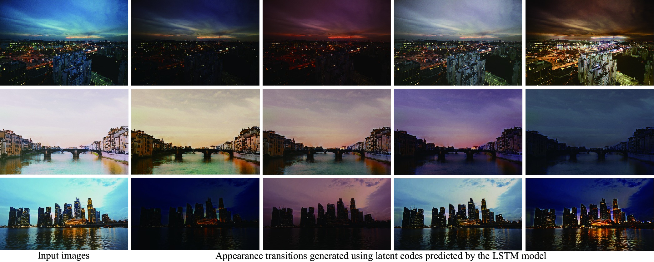
Figure 21. Appearance predictions only from input images. In each row, the latent code for the first frame is encoded using the appearance encoder, and successive latent codes are predicted recurrently by the LSTM model. Various appearance transitions are reproduced from different latent code sequences, each of which varies smoothly via latent-space interpolation. From top to bottom, the output resolutions are $1,024\times 683$, $1,080\times 720$, and $700\times 394$. Input photos: :DC Snapshots/Unsplash.com, Domenico Loia/Unsplash.com, and Shih et al. [2013].

Appendix C Generalizability

Whereas most of our results contain cloud-like motion and one-day appearance transition simply because time-lapse videos in available datasets typically capture such scenes, we further investigated the generalizability of our method.

Table 3. Network architecture of the LSTM model for predicting latent codes for appearance.

Component	Layers	Specifications
	fc	Linear(128)
LSTM model	lstm	LSTM(128)
	fc	Linear(8)

Figure 22 compares gait motions generated from the KTH dataset [Schüldt et al., 2004]. Our method yields more plausible results than [Xue et al., 2016; Denton and Birodkar, 2017]. The quality of our first-half frames is comparable to that of the state-of-the-art [Li et al., 2018]. Meanwhile, our latter-half frames indicate that there is room for improvement in the prediction of which leg precedes next after the leg-crossed pose. Modeling long-term dependency to handle such a situation is left for future work.

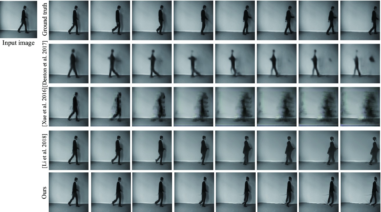
Figure 22. Comparison of gait motions generated from the KTH dataset [Schüldt et al., 2004].

Figure 23 compares season transitions into winter, generated from the transient attribute dataset [Laffont et al., 2014]. Our transition sequences contain more wider variations in spatially-local appearance and are more faithful to the target images than those of Photoshop Match Color, even in different times of the day.

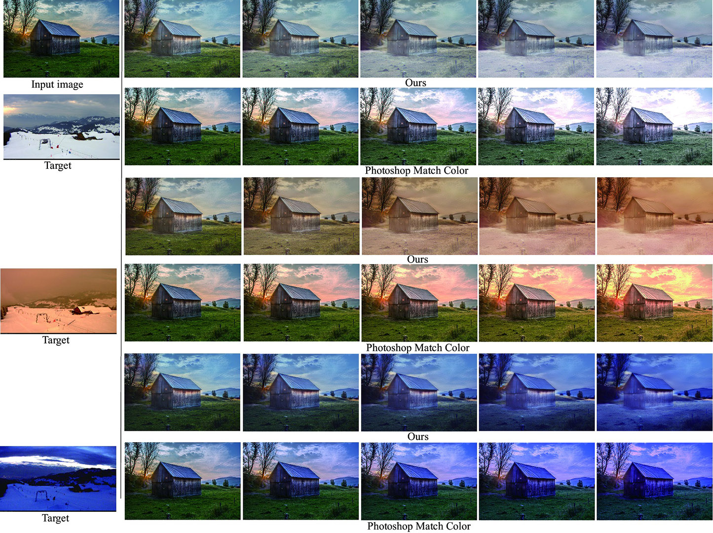
Figure 23. Comparison of season transitions into winter, generated from the transient attribute dataset [Laffont et al., 2014]. Input photo: Kevin Jarrett/Unsplash.com.

Appendix D User study

We conducted a user study for subjective validation of the plausibility of our results. We compared our method with commercial software (Plotagraph, After Effects, and Photoshop) that requires manual annotations (e.g., static and movable regions plus fine flow directions) as well as the previous methods [Xiong et al., 2018; Li et al., 2018]. We used 20 different scenes (ten for comparisons with the previous methods and the other ten for commercial software). For fair comparisons with the previous methods [Xiong et al., 2018; Li et al., 2018], we made their results looped in the same way as ours and minified our results to the same size ($128\times 128$) as their results. For comparisons with commercial software, we collected manually-created animations from Youtube and Vimeo, and generated our results from the same input images. Because the collected animations do not contain appearance transition, we created two more results containing only appearance transition using Photoshop Match Color. The evaluation criteria are i) plausibility w.r.t. motion and appearance transition for motion-added animations and ii) faithfulness against target images for appearance-only animations (i.e., comparisons with Photoshop Match Color); appearance-only results are highly plausible in any methods, and thus we omitted plausibility for them. We requested 11 subjects to score video clips on a 1-to-4 scale ranging from “implausible (or unfaithful)” to “plausible (or faithful)” after they watch each clip only once. The movie used in this user study is submitted as a supplemental material.

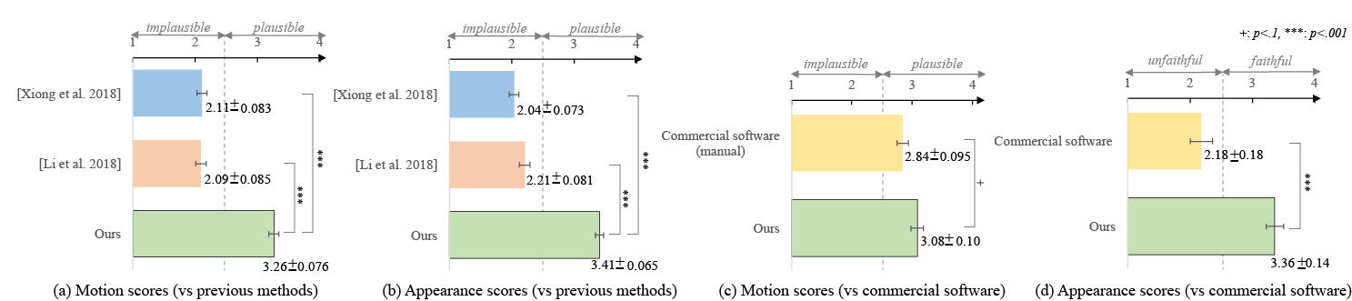
Figure 24. Statistics of our user study. The graphs indicate that our method yields more plausible results than the previous methods and commercial software. The error bars represent standard errors. The results marked with * show statistically-significant differences (paired t-test).

Figure 24 summarizes the statistics of the user study. The graphs in Figure 24 (a) and (b) indicate that our method significantly outperforms the previous methods in terms of plausibility of motion and appearance. In Figure 24 (c), we can confirm that our motion scores are slightly better than those manually created using commercial software. Figure 24 (d) shows that our method can reproduce target styles more faithfully and can handle wider variations in appearance than commercial software, as demonstrated in Figures 12, 13, and 23.