Transport on a topological insulator surface with a time-dependent magnetic barrier

Abstract

We study transport across a time-dependent magnetic barrier present on the surface of a three-dimensional topological insulator. We show that such a barrier can be implemented for Dirac electrons on the surface of a three-dimensional topological insulator by a combination of a proximate magnetic material and linearly polarized external radiation. We find that the conductance of the system can be tuned by varying the frequency and amplitude of the radiation and the energy of an electron incident on the barrier providing us optical control on the conductance of such junctions. We first study a $\delta$-function barrier which shows a number of interesting features such as sharp peaks and dips in the transmission at certain angles of incidence. Approximate methods for studying the limits of small and large frequencies are presented. We then study a barrier with a finite width. This gives rise to some new features which are not present for a $\delta$-function barrier, such as resonances in the conductance at certain values of the system parameters. We present a perturbation theory for studying the limit of large driving amplitude and use this to understand the resonances. Finally, we use a semiclassical approach to study transmission across a time-dependent barrier and show how this can qualitatively explain some of the results found in the earlier analysis. We discuss experiments which can test our theory.

I Introduction

Topological insulators (TI) have been studied extensively both theoretically and experimentally due to their remarkable physical and mathematical properties (see Refs. [hasan, ; qi, ] for reviews). These are materials in which the bulk states are separated from the Fermi energy by a finite gap and therefore do not contribute to electronic transport at low temperatures; however, there are states at the boundaries which are gapless (if certain symmetries like time-reversal are not broken), and they participate in transport. In reality, many TIs have some bulk conductance because the Fermi energy lies within a bulk conduction band. However, an appropriate amount of doping can produce ideal TIs where the bulk conductance is very small brahlek ; kushwaha . Further, the number of boundary states with a given momentum is given by a topological invariant which characterizes the bulk states. In three-dimensional (3D) topological insulators such as Bi₂Se₃ and Bi₂Te₃, the boundaries are surfaces, and the surface electrons are typically governed by the Hamiltonian of a single massless Dirac particle in two spatial dimensions. Further, the Hamiltonians exhibit spin-momentum locking, so that the linear momentum and the spin angular momentum of an electron are perpendicular to each other. If time-reversal symmetry is not broken (by, say, magnetic impurities), the spin-momentum locking leads to ballistic transport; this is because scattering from a non-magnetic impurities cannot flip the spin of an electron and therefore cannot change its momentum. The application of an in-plane magnetic field which has a Zeeman coupling to the spin or, equivalently, the presence of a proximate magnetic material which induces in plane Zeeman magnetization, alters the spin-momentum locking of the Dirac electrons yoko ; sm1 . It has been shown in Ref. sm1, that the presence of such proximate magnetic material over a strip of finite width can cut off conductance across it for sufficiently strong induced magnetization. This allows one to implement a magnetic switch and achieve magnetic control over electric current in these materials utilizing spin-momentum locking of Dirac quasiparticles.

The effects of periodic driving of quantum many-body systems is another subject which has been studied extensively for about a decade from many points of view (for reviews, see Refs. [rudner, ; nathan, ; cayssol, ; goldman, ; eckardt, ; bukov, ; mikami, ]). Such periodic driving can be used to change the band structure of a material (giving rise to phenomena such as dynamical freezing das ; bhat ; hegde ; pekker ; nag1 ; nag2 ; agarwala1 ), generate boundary modes and induce dynamical topological transitions by changing a non-topological system to a topological one rudner ; cayssol ; mikami ; oka ; inoue ; kita1 ; kita2 ; gu ; lindner ; morrell ; katan ; delplace ; tong ; thakur1 ; thakur2 ; usaj ; kundu1 ; carp ; alessio ; xiong ; loss ; mukh1 ; mukh2 ; zhou , produce novel steady states which cannot appear in time-independent systems nathan , and control electronic transport bukov ; kundu2 ; agarwala2 .

In this paper, we will be interested in the last aspect of periodic driving, namely its role on the electric transport. More precisely, we will study what happens when a magnetic barrier which is periodically varying in time is placed on the surface of a 3D TI like Bi₂Se₃. Such a barrier can be realized in these materials by applying an in-plane magnetic field (which induces a static Zeeman magnetization) and a linearly polarized light (which provides the time varying part) over a region of width $L$. A schematic picture of the system is shown in Fig. 1. We will see that the conductance of this system, in the presence of such a barrier, exhibits a number of interesting features, such as prominent peaks and dips, as the different system parameters are varied. Moreover, such a barrier provides a route to optical (electromagnetic) control over electric current in such junctions; we show that the conductance of such a junction can be tuned by controlling the amplitude and frequency of the applied light even in the absence of a static Zeeman field. We note that an analogous study for the case of an oscillating potential barrier was carried out in Ref. mondal, ; however, the optical control of conductance that we find in our study has not been obtained earlier.

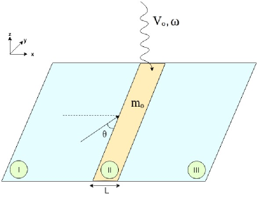
Figure 1: Schematic picture of the system showing the top surface of a TI, with a static magnetic barrier of strength $m_{0}$ and electromagnetic radiation with frequency $\omega$ and amplitude $V_{0}$ which is incident on the barrier. The barrier has a width $L$ (region $II$), and an electron comes in from region $I$ with an angle of incidence $\theta$.

The plan of this paper is as follows. In Sec. II we study the effect of a $\delta$-function magnetic barrier which has both a constant term $m_{0}$ and a term which oscillates sinusoidally with an amplitude $\alpha$ and frequency $\omega$; we take the field to point along the $\hat{x}$ direction. The $\delta$-function nature of the barrier allows a simpler analysis of the problem than the more realistic case of a finite-width barrier which is discussed in the next section. We find that the $\delta$-function leads to a non-trivial matching condition for the wave function on the left and right edges of the barrier. Assuming that an electron is incident on the barrier from the left with an energy $E_{0}$ and angle of incidence $\theta$, we will use the matching condition to derive the transmission amplitudes in the different Floquet bands and hence the transmitted current on the right of the barrier. Integrating this over $\theta$ gives the differential conductance $G$. We then present our numerical results for the transmitted current and $G$ as a function of the parameters $m_{0}$, $\alpha$, $\omega$ and $E_{0}$. Several interesting features are seen, such as kinks in the transmitted current at certain values of $\theta$ for intermediate values of $\omega$ and peaks in $G$ at certain values of $m_{0}$ for small values of $\omega$. We provide simple explanations for these features and for the results obtained in some limits of the problem such as small and large values of $\omega$. In Sec. III, we study a time-dependent magnetic barrier which has a finite width $L$; the field is taken to consist of a constant $m_{0}$ and an oscillating term with an amplitude $V_{0}$ and frequency $\omega$. We examine surface plots of $G$ as a function of $V_{0}$ and $m_{0}$ for various values of $\omega$. We find that $G$ is peaked along the line $m_{0}=V_{0}$ for small $\omega$ and shows resonance-like features for a discrete set of values of $V_{0}$ when $\omega$ is large and $m_{0}$ is small. We show that the conductance of a time-dependent barrier with parameters $(m_{0},V_{0},\omega)$ can be mapped to that of a time-independent barrier with a single parameter $m_{eff}$; we find that $m_{eff}$ approaches a constant for large $\omega$, where the constant depends on $(m_{0},V_{0})$. We also find that when $E_{0}$ and $\omega$ are large and are related as $E_{0}=\hbar\omega/2$, there are prominent dips in $G$. We analyze how the width and magnitude of the dips depend on the parameters $V_{0}$ and $L$. We provide a detailed study of the behavior of $G$ as a function of $m_{0}$ and $V_{0}$ at both high and low frequencies, and show that for small or zero $m_{0}$, one can tune $V_{0}$ to control $G$ in these systems. This shows that these junctions can operate as optically controlled switches. To study this more carefully, we carry out a detailed investigation of the dependence of $G$ on $V_{0}$ and $\omega$, for a fixed value of $E_{0}$ and $L$, taking $m_{0}=0$. We find that for $\omega/V_{0}\gtrsim 0.83$, there are curves in the $(V_{0},\omega)$ plane along which there are resonances and $G$ is particularly high; the spacing between these curves is proportional to $1/L$. For $\omega/V_{0}\lesssim 0.83$, the conductance is small everywhere; however, it is particularly small along certain straight lines. We present a Floquet perturbation theory which can explain both the resonances and the lines of very small conductances. We summarize our results and discuss possible experimental tests in Sec. IV. The paper ends with two appendices. In Appendix A we briefly recall the basics of Floquet theory and how the Floquet eigenstates and eigenvalues can be found. In Appendix B, we present a completely different approach to the problem of a time-dependent magnetic barrier. While Secs. II and III considered a spin-1/2 electron, we consider the large-spin limit in this appendix and study the semiclassical equations of motion for the trajectory of such a particle moving in two dimensions in the presence of an electromagnetic field. Using this approach, we are able to qualitatively understand some features of the surface plots of $G$ versus $(V_{0},m_{0})$ presented in Sec. III.

II $\delta$-function magnetic barrier

In this section, we will study the effect of a magnetic barrier present on the top surface of a three-dimensional TI hasan ; qi . The Hamiltonian for electrons on the surface (taken to be the $x-y$ plane) is known to have the form of a massless Dirac equation with spin-momentum locking, namely,

$$H~{}=~{}-i\hbar v~{}\left[\sigma^{x}\frac{\partial}{\partial y}~{}-~{}\sigma^{y}\frac{\partial}{\partial x}\right],$$ (1)

where $v$ is the velocity, $\sigma^{a}$ denote Pauli matrices, and the wave function $\psi(x,y,t)$ has two components. In the well-known TI Bi₂Se₃, it is known qi that $\hbar v=0.333$ eV-nm.

We now consider a magnetic barrier which has the form of a $\delta$-function located along the line $x=0$; the barrier strength will be taken to have both a constant term and a term which oscillates in time with a frequency $\omega$ and an amplitude $\alpha$. We will assume that the magnetic field associated with the barrier points in the $\hat{x}$ direction; we can then ignore the coupling of the field to the orbital motion of the electrons since they are constrained to move in the $x-y$ plane and therefore cannot have cyclotron orbits perpendicular to the field direction. Hence we only have a Zeeman coupling of the field to the electron spin. The Hamiltonian will therefore take the form

$$H~{}=~{}\hbar v~{}\left[\sigma^{x}\{-i\frac{\partial}{\partial y}~{}+~{}[m_{0}~{}+~{}\alpha~{}\cos(\omega t)]~{}\delta(x)\}~{}+~{}i\sigma^{y}\frac{\partial}{\partial x}\right],$$ (2)

where for an applied field $B=B_{0}+B_{1}\cos(\omega t)\hat{x}$, $m_{0}[\alpha]=g\mu_{B}B_{0}[B_{1}]/(\hbar vk_{0})$, $g$ is the gyromagnetic ratio, $\mu_{B}$ is the Bohr magneton, and $k_{0}$ is the inverse of a typical length scale (for instance, a typical barrier width of the order of 20 nm as stated in Sec. III.1). We note that $m_{0}$ and $\alpha$ are dimensionless quantities. We also point out that the oscillation term may be generated via coupling of $H$ to linearly polarized vector potential given by $A=A_{0}\cos(\omega t)\hat{y}$ in which case $\alpha=eA_{0}/(\hbar vk_{0})$, where $e$ is the electron charge. This is a consequence of the fact that the coupling to the magnetic barrier appears in Eq. (2) as an addition to $p_{y}=-i\hbar\partial/\partial y$ and therefore acts as a vector potential in the $y$ direction.

Given that the wave function satisfies

$$i\hbar\frac{\partial\psi(x,y,t)}{\partial t}~{}=~{}H\psi(x,y,t),$$ (3)

we can derive the matching condition that $\psi$ must satisfy at $x=0$ due to the $\delta$-function in Eq. (2). To do this, we assume that

$$\psi~{}=~{}\psi_{0}(y,t)~{}e^{f(x)}$$ (4)

in the vicinity of $x=0$, where $f(x)$ may have a discontinuity at $x=0$. We then integrate the two sides of Eq. (3) from $x=-\epsilon$ to $x=+\epsilon$, and take the limit $\epsilon\to 0$. This gives

$$i\sigma^{y}~{}[f(x=0+)~{}-~{}f(x=0-)]~{}+~{}\sigma^{x}~{}[m_{0}~{}+~{}\alpha\cos(\omega t)]~{}=~{}0,$$ (5)

which implies that

$$f(x=0+)~{}-~{}f(x=0-)~{}=~{}\sigma^{z}~{}[m_{0}~{}+~{}\alpha\cos(\omega t)].$$ (6)

Thus the wave function will have a discontinuity at $x=0$ given by

$$\psi_{x=0^{+}} = e^{[m_{0}+\alpha~{}\cos(\omega t)]\sigma^{z}}\psi_{x=0^{-}},$$

$${\rm namely,}~{}~{}~{}\psi_{x=0^{+}} = \begin{pmatrix}e^{m_{0}+\alpha\cos(\omega t)}&0\vspace{0.5cm}\\ 0&e^{-m_{0}-\alpha\cos(\omega t)}\end{pmatrix}\psi_{x=0^{-}}.$$ (7)

We can now use the identity

$$e^{\alpha\cos\theta}~{}=~{}\sum_{n=-\infty}^{\infty}~{}I_{n}(\alpha)~{}e^{-in\theta},$$ (8)

where $I_{n}(\alpha)$ is the modified Bessel function abram . (These functions satisfy $I_{n}(\alpha)=I_{-n}(\alpha)$ and $I_{n}(-\alpha)=(-1)^{n}I_{n}(\alpha)$). Hence Eq. (7) takes the form

$$\psi_{x=0^{+}}~{}=~{}\begin{pmatrix}e^{m_{0}}\sum\limits_{n=-\infty}^{\infty}I_{n}(\alpha)e^{-in\omega t}&0\vspace{0.5cm}\\ 0&e^{-m_{0}}\sum\limits_{n=-\infty}^{\infty}I_{n}(-\alpha)e^{-in\omega t}\end{pmatrix}~{}\psi_{x=0^{-}}.$$ (9)

II.1 Transmitted particle current

We now assume that an electron is incident on the magnetic barrier from the left ($x<0$) with energy $E_{0}>0$ (measured with respect to the Dirac point) and momentum $(k_{x,0},k_{y})$. (These satisfy the dispersion relation $E_{0}=v\sqrt{k_{x,0}^{2}+k_{y}^{2}}$). We will calculate the probabilities of reflection and transmission from the time-dependent barrier.

We now use the matching condition in Eq. (9). In our problem, $\psi_{x=0^{+}}=\psi_{t}$ is the transmitted wave, while $\psi_{x=0^{-}}$ is given by the sum of the incident wave $\psi_{i}$ and the reflected wave $\psi_{r}$. The incident wave is given by

$$\frac{1}{\sqrt{2}}~{}\begin{pmatrix}1\vspace{0.5cm}\\ \dfrac{E_{0}}{v~{}(k_{y}+ik_{x,0})}\end{pmatrix},$$ (10)

where $k_{x,0}=\sqrt{(E_{0}/v)^{2}-k_{y}^{2}}$. This gives rise to reflected and transmitted waves at $x=0$ due to the presence of the $\delta$-function. We can see from Eq. (62) that the allowed energies of these are given by the energies of all the Floquet modes, namely,

$$E_{n}~{}=~{}E_{0}~{}+~{}n\hbar\omega,$$ (11)

where $n$ is an integer which can take any value from $-\infty$ to $\infty$; the modes with $n\neq 0$ are called side bands. (Note that $E_{n}$ may be either positive or negative). Since the $\delta$-function is independent of the $y$ coordinate, the momentum $k_{y}$ is a good quantum number. For each energy $E_{n}$, the corresponding eigenfunction is given by

$$\frac{1}{\sqrt{2}}\begin{pmatrix}1\vspace{0.5cm}\\ \dfrac{E_{n}}{v(k_{y}+ik_{x,n})}\end{pmatrix}~{}~{}~{}\text{with}~{}~{}~{}k_{x,n}~{}=~{}\pm\sqrt{(E_{n}/v)^{2}~{}-~{}k_{y}^{2}}.$$ (12)

The $\pm$ sign for $k_{x,n}$ in Eq. (12) is fixed by the requirement that the group velocity $v_{g}=\partial E_{n}/\partial k_{x,n}$ should be positive for the transmitted wave in the region $x>0$ and negative for the reflected wave in the region $x<0$. (This holds if $k_{x,n}$ is real. If $k_{x,n}$ is imaginary, we have to choose the $\pm$ sign in such a way that the corresponding wave decays as $x\to+\infty$ or $-\infty$). Substituting the eigenfunctions in Eq. (12) in Eq. (9), we find that at $x\to 0$,

$$\begin{pmatrix}e^{m_{0}}\sum\limits_{m=-\infty}^{\infty}I_{m}(\alpha)e^{-im\omega t}&0\vspace{0.5cm}\\ 0&e^{-m_{0}}\sum\limits_{m=-\infty}^{\infty}I_{m}(-\alpha)e^{-im\omega t}\end{pmatrix}\Bigg{[}\begin{pmatrix}1\vspace{0.5cm}\\ \beta_{0}^{+}\end{pmatrix}~{}e^{-iE_{0}~{}t}~{}+~{}r_{n}\begin{pmatrix}1\vspace{0.5cm}\\ \beta_{n}^{-}\end{pmatrix}~{}e^{-iE_{n}~{}t}\Bigg{]}~{}=~{}t_{n}\begin{pmatrix}1\vspace{0.5cm}\\ \beta_{n}^{+}\end{pmatrix}~{}e^{-iE_{n}~{}t},$$ (13)

where

$$\beta_{n}^{\pm}~{}=~{}\dfrac{E_{n}}{v(k_{y}\pm ik_{x,n})},$$ (14)

and $r_{n}$ and $t_{n}$ are the reflection and transmission amplitudes respectively for the $n$-th Floquet mode with energy $E_{n}$. The superscript $\pm$ in $\beta_{n}^{\pm}$ indicates if the wave is traveling in the positive or negative $x$ direction.

Given the Hamiltonian in Eq. (2), we can use the equation of continuity to show that the particle current operator is given by

$$J_{x}~{}=~{}-~{}v\sigma^{y}.$$ (15)

The charge current will be equal to the particle current multiplied by the electron charge, as we will see in Eq. (21) below. Using the eigenfunctions in Eq. (12), we find that the transmitted particle current in the band $n$ is given by

$$<J_{x}>_{n}~{}=~{}\dfrac{v^{2}|t_{n}|^{2}k_{x,n}}{E_{n}}$$ (16)

if $k_{x,n}$ is real. (If $k_{x,n}$ is imaginary, we find that $<J_{x}>_{n}=0$. This is because when $k_{x,n}$ is imaginary, both the components of the corresponding wave function are real and hence the expectation value of $\sigma^{y}$ vanishes). Thus $E_{n}$ and $k_{x,n}$ must have the same sign in value of $<J_{x}>$ in the transmitted region in order to have a positive value of $<J_{x}>_{n}$. Similarly, $E_{n}$ and $k_{x,n}$ must have opposite signs to have a negative value of $<J_{x}>_{n}$. Now, since $E_{n}=E_{0}+n\hbar\omega$, and $e^{-in\omega t}$ form a basis for periodic functions of $t$, we can match the coefficients for each $n$ separately in Eq. (13). For each value of $n$, we obtain two equations since the wave function has two components. To solve these equations numerically, we must truncate the number of equations. If $N$ is the total number of values that the integer $n$ can take, we have $2N$ equations, and $2N$ unknown coefficients ($N$ reflection amplitudes $r_{n}$ and $N$ transmission amplitudes $t_{n}$). We can therefore numerically find the values of $r_{n}$ and $t_{n}$. Incidentally, current conservation implies that moskalets ; agarwal

$$\frac{k_{x,0}}{E_{0}}~{}=~{}\sum_{n=-\infty}^{\infty}~{}(|t_{n}|^{2}~{}+~{}|r_{n}|^{2})~{}\frac{k_{x,n}}{E_{n}}.$$ (17)

Rearranging Eqs. (13), we obtain the matrix equation

$$\begin{pmatrix}\ddots&\vdots&\vdots&\vdots&\vdots&\vdots&\vdots&\vdots&\reflectbox{$\ddots$}\\ \cdots&e^{m_{0}}I_{0}^{+}&e^{m_{0}}I_{-1}^{+}&e^{m_{0}}I_{-2}^{+}&\cdots&-1&0&0&\cdots\\ \cdots&e^{m_{0}}I_{1}^{+}&e^{m_{0}}I_{0}^{+}&e^{m_{0}}I_{-1}^{+}&\cdots&0&-1&0&\cdots\\ \cdots&e^{m_{0}}I_{2}^{+}&e^{m_{0}}I_{1}^{+}&e^{m_{0}}I_{0}^{+}&\cdots&0&0&-1&\cdots\\ &\vdots&\vdots&\vdots&\vdots&\vdots&\vdots&\vdots\\ \cdots&e^{-m_{0}}\beta_{-1}^{-}I_{0}^{-}&e^{-m_{0}}\beta_{0}^{-}I_{-1}^{-}&e^{-m_{0}}\beta_{1}^{-}I_{-2}^{-}&\cdots&\beta_{-1}^{+}0&0&0&\cdots\\ \cdots&e^{-m_{0}}\beta_{-1}^{-}I_{1}^{-}&e^{-m_{0}}\beta_{0}^{-}I_{0}^{-}&e^{-m_{0}}\beta_{1}^{-}I_{-1}^{-}&\cdots&0&\beta_{0}^{+}&0&\cdots\\ \cdots&e^{-m_{0}}\beta_{-1}^{-}I_{2}^{-}&e^{-m_{0}}\beta_{0}^{-}I_{1}^{-}&e^{-m_{0}}\beta_{1}^{-}I_{0}^{-}&\cdots&0&0&\beta_{1}^{+}&\cdots\\ \reflectbox{$\ddots$}&\vdots&\vdots&\vdots&\vdots&\vdots&\vdots&\vdots&\ddots\\ \end{pmatrix}\begin{pmatrix}\vdots\\ r_{-1}\\ r_{0}\\ r_{1}\\ \vdots\\ t_{-1}\\ t_{0}\\ t_{1}\\ \vdots\end{pmatrix}=-\begin{pmatrix}\vdots\\ e^{m_{0}}I_{-1}^{+}\\ e^{m_{0}}I_{0}^{+}\\ e^{m_{0}}I_{1}^{+}\\ \vdots\\ e^{-m_{0}}\beta_{0}^{+}I_{-1}^{-}\\ e^{-m_{0}}\beta_{0}^{+}I_{0}^{-}\\ e^{-m_{0}}\beta_{0}^{+}I_{1}^{-}\\ \vdots\end{pmatrix}.$$ (18)

where $I^{+}_{n}$ and $I^{-}_{n}$ denote the $n$-th modified Bessel function with arguments $\alpha$ and $-\alpha$ respectively.

The total transmitted particle current is given by a sum over all bands,

$$I_{t}~{}=~{}<J_{x}>_{tot}~{}=~{}\sum\limits_{n=-\infty}^{\infty}~{}|t_{n}|^{2}\bigg{(}\dfrac{v^{2}k_{x,n}}{E_{n}}\bigg{)},$$ (19)

where the sum only runs over terms in which $k_{x,n}$ is real.

The angle of incidence of the electron coming from the left of the barrier is given by

$$\theta~{}=~{}\tan^{-1}\Big{(}\frac{k_{x}}{k_{y}}\Bigr{)},$$ (20)

where $\theta$ lies in the range $[0,\pi]$; normal incidence corresponds to $\theta=\pi/2$. The total transmitted particle current $I_{t}$ is clearly a function of $\theta$. Given $I_{t}(\theta)$, the differential conductance $G$ can be calculated as follows adithi . Suppose that the $\mu_{L}$ and $\mu_{R}$ denote the chemical potentials of the left and right leads assumed to be at $x\to-\infty$ and $x\to\infty$ respectively; the chemical potential $\mu$ in a lead is related to the voltage $V$ applied to that lead as $\mu=qV$, where $q$ is the charge of the electron. In the zero-bias limit, $\mu_{L},~{}\mu_{R}~{}\to~{}E_{0}$, the differential conductance is given by

$$G~{}=~{}\frac{dI}{dV}~{}=~{}\frac{q^{2}WE_{0}}{(2\pi v\hbar)^{2}}~{}\int_{0}^{\pi}d\theta~{}I_{t}(\theta),$$ (21)

where $W$ is the width of the system in the $y$ direction (assumed to be much larger that the wavelength $\sim\hbar v/E_{0}$ of the electrons). It is convenient to define a quantity $G_{0}$ which is the maximum possible value of $G$; this arises when the total transmitted current has the maximum possible value given by $I_{t}(\theta)=v^{2}k_{x,0}/E_{0}=v\sin\theta$. The conductance in this case is given by

$$G_{0}~{}=~{}\frac{q^{2}WE_{0}}{2v(\pi\hbar)^{2}}.$$ (22)

In the figures presented below, we will plot the dimensionless ratio $G/G_{0}=(1/2v)\int_{0}^{\pi}d\theta I_{t}(\theta)$ whose maximum value is 1.

II.2 Numerical results

We now present our numerical results as a function of the different parameters of the system. In our calculations, we have generally taken $E_{0}=2$ in units of $0.01$ eV (so that it is much smaller than the bulk gap of $0.56$ eV in Bi₂Se₃, ensuring that there is no contribution to the current from the bulk states). Hence $k=\sqrt{k_{x}^{2}+k_{y}^{2}}$ will have the value $E_{0}/(\hbar v)=0.02/0.333=0.06$ nm^-1 in Bi₂Se₃. The values of $\omega$ will be taken to be in units of $0.01$ eV/$\hbar$ $\simeq 15.2$ THz.

II.2.1 Transmitted particle current as a function of $\theta$

Figure 2 shows the total transmitted particle current as a function of the angle of incidence $\theta$, for different values of $m_{0}$, $\alpha$ and $\omega$. We observe that there are kinks in some of the plots. These occur because at those values of $\theta$, the value of $k_{x,n}$ changes from real to imaginary for some value of $n$; as a result the contribution to the transmitted current from that side band becomes zero. Given that $v\hbar k_{x,n}=\pm\sqrt{(E_{0}+n\hbar\omega)^{2}-v^{2}\hbar^{2}k_{y}^{2}}$ $=\pm\sqrt{(E_{0}+n\hbar\omega)^{2}-E_{0}^{2}\cos^{2}\theta}$, we see that $k_{x,n}$ becomes imaginary when

$$\cos\theta~{}=~{}\pm~{}\left(1~{}+~{}\dfrac{n\hbar\omega}{E_{0}}\right).$$ (23)

It can be checked that the kinks appearing in Fig. 2 exactly coincide with the values of $\theta$ corresponding to different values of $n$ in the above equation. For small and large values of $\omega$, kinks do not appear. For large $\omega$, there is no value of $n$ which satisfies the condition in Eq. (23). For small $\omega$, the values of $\theta$ which satisfy the condition lie close to glancing angles (0 and $\pi$) where the transmitted current is always small; hence kinks in the current are not observable.

For $m_{0}=0$, Fig. 2 shows that the transmitted particle current is symmetric about $\theta=\pi/2$. This is because of the following symmetry of the Hamiltonian in Eq. (2) when $m_{0}=0$. Replacing $-i\partial/\partial y\to k_{y}=k\cos\theta$, we see that changing $\theta\to\pi-\theta$ and shifting the time $t\to t+\pi/\omega$, we get a new Hamiltonian which is related to the old Hamiltonian by the unitary transformation $H\to\sigma^{y}H\sigma^{y}$. According to Floquet theory, physical quantities like the transmitted current are invariant under time shifts. Hence the current must be invariant under $\theta\to\pi-\theta$.

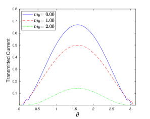
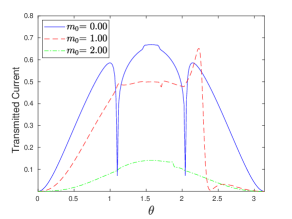
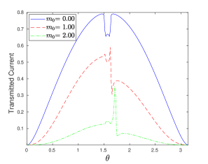
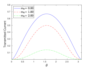
Figure 2: Transmitted particle current as a function of angle of incidence for different values of $m_{0}$, $E_{0}=2,~{}\alpha=1$, and $\omega$ equal to (a) 0.01, (b) 1.1, (c) 2.1, and (d) 5.1.

II.2.2 Differential conductance as a function of $m_{0}$

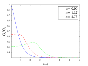
Figure 3: $G/G_{0}$ as a function of $m_{0}$ for different values of $\alpha$, with $E_{0}=2$, and $\omega$ equal to $0.01$.

Figure 3 shows the dimensionless differential conductance $G/G_{0}$ as a function of $m_{0}$, for different values of $\alpha$. If $\alpha$ is not too small, we see that there are peaks in the conductance, and their locations move with $\alpha$. This can be qualitatively understood as follow, particularly for the lowest value of $\omega=0.01$. The strength of the magnetic barrier is given by $m_{0}+\alpha\cos(\omega t)$. When $m_{0}=\pm\alpha$, the barrier strength stays close to zero for a long time since $\pm 1$ correspond to the extreme values of $\cos(\omega t)$; this is particularly true if $\omega$ is small. The barrier strength being close to zero gives rise to a large value of the transmitted particle current and therefore of the conductance.

For large values of $m_{0}$, we see that the conductance goes to zero for all values of $\alpha$ and $\omega$. This can be understood from Eq. (9). Large $m_{0}$ means that $e^{-m_{0}}$ and therefore the lower component of $\psi_{x=0+}$ is small. Hence the current, which is proportional to $\psi_{x=0+}^{\dagger}\sigma^{y}\psi_{x=0+}$, will be small.

II.2.3 Differential conductance as a function of $\alpha$

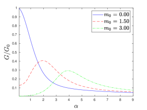
Figure 4: $G/G_{0}$ as a function of $\alpha$ for different values of $m_{0}$, with $E_{0}=2$ and $\omega=1.1$.

Figure 4 shows the dimensionless differential conductance $G/G_{0}$ as a function of $\alpha$, for different values of $m_{0}$ and $\omega$. Once again we see that there are peaks in the conductance when $\alpha$ is close to $m_{0}$; this can be understood in the same way as the peaks in Fig. 3. For large values of $\alpha$, we see in Fig. 5 that the conductance approaches a constant value which is almost independent of $m_{0}$. This can be understood since the magnetic barrier strength is $m_{0}+\alpha\cos(\omega t)$; if $\alpha\gg m_{0}$, the barrier strength is dominated by the $\alpha$ term. We note that for both small and intermediate $\omega$ and small $m_{0}$, $G$ can be substantially reduced by increasing the intensity of the applied radiation $\alpha$. This provides optical control over the conductance; we will analyze this point in more detail in the next section.

II.2.4 Small $\omega$ limit

Next, we look at the adiabatic limit $\hbar\omega\ll E_{0}$. Since the barrier strength varies very slowly with time in this limit, we can estimate the total transmitted particle current value by studying the Hamiltonian at an equispaced sequence of frozen times covering one time period $T$, and then averaging over the results for all these times. Thus by solving a sequence of problems with no time dependence, we expect to obtain a good approximation of the time-dependent problem. The time-dependent term in the barrier strength is $\alpha\cos(\omega t)$. Denoting $\phi=\omega t$, we fix $\phi$ at $N$ equispaced values, $\phi_{j}$, in the range 0 to $2\pi$, and find the total transmitted current $I(\phi_{j})$ for each value of $j$. We then calculate the averaged current

$$I_{avg}~{}=~{}\dfrac{\sum\limits_{j=1}^{N}I(\phi_{j})}{N},$$ (24)

and check how well this compares with the result for the time-dependent problem. The results are shown in Fig. 5. As we can see from the figure, the averaging approximation works well for $\omega=0.01$ which is much smaller than $E_{0}/\hbar$. When $\omega$ is larger than $E_{0}/\hbar$, we observe a significant difference between from the averaged current and the actual current obtained for the time-dependent system.

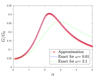
Figure 5: $G/G_{0}$ as a function of $\alpha$. The current obtained by solving the time-dependent problem is shown by the solid blue curve (for $\omega=0.01$) and dashed green curve (for $\omega=2.1$), while the value obtained by averaging over $N=100$ equispaced values of $\phi$ is shown by the red circles. The averaged results (red) agree well with the results for $\omega=0.01$ (blue) which is in the adiabatic regime, but do not agree with the results for $\omega=2.1$ (green).

II.2.5 Large $\omega$ limit

We now look at the opposite limit where $\hbar\omega\gg E_{0}$. Since the energy in the $n$-th band is given by $E_{n}=E_{0}+n\hbar\omega$, the gap between successive side bands is much larger that $E_{0}$ in this limit. Hence we do not expect the side bands to contribute much to the current. Also, the momenta $k_{x,n}$ and $k_{y}$ are related to $E_{n}$ as $k_{x,n}=\pm(1/v)\sqrt{E_{n}^{2}-v^{2}k_{y}^{2}}$; we can ignore $k_{y}$ in this expression if $E_{n}$ is very large. Thus $k_{x,n}\approx\pm E_{n}/v$. Eq. (12) then implies that the eigenfunctions of the side bands become independent of $n$, and we get

$$\psi_{n}=\frac{1}{\sqrt{2}}\begin{pmatrix}1\vspace{0.5cm}\\ \dfrac{E_{n}}{ivk_{x,n}}\end{pmatrix},$$ (25)

for $n\neq 0$, where we have ignored $k_{y}$. Simplifying this, we obtain

$$\psi_{n,t}=\frac{1}{\sqrt{2}}\begin{pmatrix}1\vspace{0.5cm}\\ -i\end{pmatrix}~{}~{}~{}\text{and}~{}~{}~{} \psi_{n,r}=\frac{1}{\sqrt{2}}\begin{pmatrix}1\vspace{0.5cm}\\ i\end{pmatrix}$$ (26)

as the approximate wave functions in the large $\omega$ limit for the transmitted and reflected waves respectively for $n\neq 0$. Using these wave functions, we solve the equations analogous to Eq. (13) to find $r_{n}$ and $t_{n}$ and hence the total transmitted particle current. (Note that since the wave functions in Eq. (26) do not depend on $\omega$, the transmitted current and conductance become independent of $\omega$ in the large $\omega$ limit). Figure 6 shows a comparison between the results obtained by this approximation and the exact result. We see that the agreement is very good when $\omega=100.1\gg E_{0}/\hbar$ but deviates significantly when $\omega=2.1$ is comparable to $E_{0}/\hbar$.

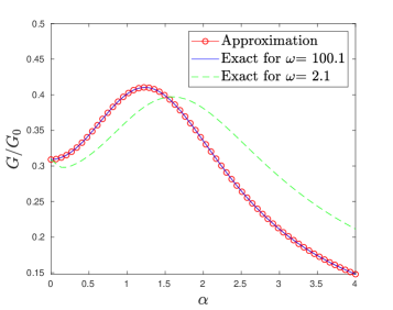
Figure 6: $G/G_{0}$ as a function of $\alpha$. The solid blue and dashed green curves show the currents obtained by solving the time-dependent problem for $\omega$ equal to $100.1$ and $2.1$ respectively. The red circles show the approximate solution obtained by using the wave functions in Eq. (26). We have taken $E_{0}=2$ and $m_{0}=1$.

III Finite-width magnetic barrier

In this section, we study the effects of a time-dependent magnetic barrier which has a finite width; we will assume that the barrier lies in the region $0\leq x\leq L$. The incident and reflected waves lie in region $I$ where $x<0$, while the transmitted wave lies in region $III$ where $x>0$. In region $II$ where $0\leq x\leq L$, the wave function satisfies the equation

$$i\hbar\dfrac{\partial\psi}{\partial t}~{}=~{}\hbar v~{}[k_{y}\sigma^{x}~{}+~{}i\sigma^{y}\frac{\partial}{\partial x}~{}+~{}\{m_{0}+V_{0}\cos(\omega t)\}~{}\sigma^{x}]~{}\psi.$$ (27)

We note that $m_{0}=g\mu_{B}B_{0}/(\hbar v)$ and $V_{0}=eA_{0}/(\hbar v)$ have the dimensions of inverse length. We now assume that the solution of Eq. (27) is of the form

$$\psi~{}=~{}\sum_{n=-\infty}^{\infty}~{}\begin{pmatrix}\alpha_{n}\\ \beta_{n}\end{pmatrix}e^{i(k^{\prime}_{x}x~{}+~{}k^{\prime}_{y}y~{}-~{}E_{n}t/\hbar)},$$ (28)

where $E_{n}=E_{0}+n\hbar\omega$, $k^{\prime}_{y}=k_{y}+m_{0}$, and $k^{\prime}_{x}$ will be determined as described below. Equating coefficients of $e^{-in\omega t}$ on the two sides of Eq. (27), we obtain the following equations

$$-i\hbar vk^{\prime}_{y}\alpha_{n}~{}-~{}\dfrac{i\hbar vV_{0}}{2}(\alpha_{n+1}~{}+~{}\alpha_{n-1})~{}+~{}iE_{n}\beta_{n} = \hbar vk^{\prime}_{x}\alpha_{n}$$

$$~{}i\hbar vk^{\prime}_{y}\beta_{n}~{}+~{}\dfrac{i\hbar vV_{0}}{2}(\beta_{n+1}+\beta_{n-1})~{}-~{}iE_{n}\alpha_{n} = \hbar vk^{\prime}_{x}\beta_{n}.$$ (29)

If we truncate the above equations by keeping only $N$ bands, then Eqs. (29) give an eigenvalue equation for $k^{\prime}_{x}$ with $2N$ possible eigenvalues; the eigenvalue equation looks as follows.

$$\begin{pmatrix}\ddots&\vdots&\vdots&\vdots&\vdots&\vdots&\vdots&\vdots&\reflectbox{$\ddots$}\\ \cdots&-i\hbar vk^{\prime}_{y}&iE_{-1}&-\frac{i\hbar vV_{0}}{2}&0&0&0&\cdots\\ \cdots&-iE_{-1}&i\hbar vk^{\prime}_{y}&0&\frac{i\hbar vV_{0}}{2}&0&0&\cdots\\ \cdots&-\frac{i\hbar vV_{0}}{2}&0&-i\hbar vk^{\prime}_{y}&iE_{0}&-\frac{i\hbar vV_{0}}{2}&0&\cdots\\ \cdots&0&\frac{i\hbar vV_{0}}{2}&-iE_{0}&i\hbar vk^{\prime}_{y}&0&\frac{i\hbar vV_{0}}{2}&\cdots\\ \cdots&0&0&-\frac{i\hbar vV_{0}}{2}&0&-i\hbar vk^{\prime}_{y}&iE_{1}&\cdots\\ \cdots&0&0&0&\frac{i\hbar vV_{0}}{2}&-iE_{1}&i\hbar vk^{\prime}_{y}&\cdots\\ \reflectbox{$\ddots$}&\vdots&\vdots&\vdots&\vdots&\vdots&\vdots&\vdots&\ddots\\ \end{pmatrix}\begin{pmatrix}\vdots\\ \alpha_{-1}\\ \beta_{-1}\\ \alpha_{0}\\ \beta_{0}\\ \alpha_{1}\\ \beta_{1}\\ \vdots\end{pmatrix}~{}=~{}\hbar vk^{\prime}_{x}~{}\begin{pmatrix}\vdots\\ \alpha_{-1}\\ \beta_{-1}\\ \alpha_{0}\\ \beta_{0}\\ \alpha_{1}\\ \beta_{1}\\ \vdots\end{pmatrix}.$$ (30)

After finding the different eigenvalues $k^{\prime}_{x}$, denoted by $k^{\prime}_{x,j}$, and the corresponding values of $\alpha_{n}$ and $\beta_{n}$ denoted by $\alpha_{n,j}$ and $\beta_{n,j}$, we proceed to find the reflection and transmission amplitudes by matching wave functions at $x=0$ and $L$. At $x=0$, we have

$$\begin{pmatrix}1\\ e^{-i\theta}\end{pmatrix}\delta_{n,0}~{}+~{}r_{n}\begin{pmatrix}1\\ \beta_{n}^{-}\end{pmatrix}=\sum_{j=1}^{2N}~{}C_{j}~{}\begin{pmatrix}\alpha_{n,j}\\ \beta_{n,j}\end{pmatrix},$$ (31)

while at $x=L$, we get

$$\sum_{j=1}^{2N}~{}C_{j}~{}\begin{pmatrix}\alpha_{n,j}\\ \beta_{n,j}\end{pmatrix}e^{ik^{\prime}_{x,j}L}~{}=~{}t_{n}\begin{pmatrix}1\\ \beta_{n}^{+}\end{pmatrix}e^{ik_{x,n}L},$$ (32)

where $k_{x,n}$ and $\beta_{n}^{\pm}$ are given in Eqs. (12) and Eq. (14) respectively, $C_{j}$’s are the coefficients of the wave functions corresponding to different values of $k^{\prime}_{x,j}$ in region $II$, and $n$ takes $N$ possible values. The above equations give us a total of $4N$ conditions, since we have $N$ equations at both $x=0$ and $L$, and each wave function has two components. We have to use these conditions to determine $4N$ quantities, namely, the $2N$ values of $C_{j}$ and $N$ values of both $r_{n}$ and $t_{n}$. We can therefore calculate all these quantities and thus determine the transmitted particle current in the region $x>L$ using Eq. (19).

III.1 Numerical results

We now present our numerical results for the transmitted particle current and conductance. In our numerical calculations, we will take the incident energy $E_{0}=2$ in units of $0.01$ eV, and the barrier width $L=1$ in units of $\hbar v/(0.02$ eV) $\simeq 17$ nm. The values of $m_{0}$ and $V_{0}$ will be given in units of $0.01$ eV/$(\hbar v)\simeq 0.03$ nm^-1.

III.1.1 Transmitted particle current as a function of $\theta$

We recall that $\theta=\tan^{-1}(k_{x}/k_{y})$ is the angle of incidence in region $I$. Figure 7 shows the transmitted particle current as function of $\theta$, for different values of $V_{0}$ and $\omega$, with $E_{0}=2$ and $m_{0}=0$ and 1. If $\omega$ is not too large, we see kinks for certain values of $\theta$ for the same reasons as discussed for the $\delta$-function barrier. The plots are symmetric about $\theta=\pi/2$ for $m_{0}=0$ (Fig. 7 (a)), but there is no symmetry when $m_{0}\neq 0$ (Fig. 7 (b)).

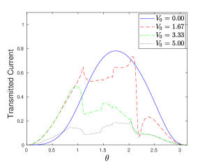
Figure 7: Transmitted particle current as a function of angle of incidence for different values of $V_{0}$, with $E_{0}=2$, $L=1$, $\omega=1.1$ and $m_{0}$ equal to (a) 0 and (b) 1.

III.1.2 Transmitted particle current as a function of $m_{0}$ and $V_{0}$

It is interesting to look at surface plots of the dimensionless differential conductance $G/G_{0}$ for different values of $\omega$, with $E_{0}=2$ and $L=1$. These are shown in Fig. 8 for $\omega=0.01,~{}1.1,~{}10.1$ and $40.1$.

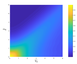
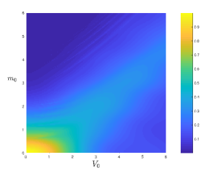
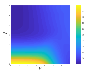
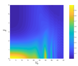
Figure 8: Surface plots of $G/G_{0}$ as a function of $V_{0}$ and $m_{0}$, for $E_{0}=2$, $L=1$, and $\omega$ equal to (a) $0.01$, (b) $1.1$, (c) $10.1$, and (d) $40.1$.

For the smallest value of $\omega=0.01$, we see that the current is maximum around the line $m_{0}=V_{0}$. This can be understood by an argument similar to the one used to understand the positions of the peaks in Fig. 3. If $\omega$ is small, the strength of the magnetic barrier, given by $m_{0}+V_{0}\cos(\omega t)$ stays close to its extreme values of $m_{0}\pm V_{0}$ for a long time. For instance, if $m_{0}=V_{0}$, an expansion of $t$ around the time $t_{0}=\pi/\omega$ gives $\hbar v[m_{0}+V_{0}\cos(\omega t)]~{}\simeq~{}\hbar vm_{0}w^{2}(t-t_{0})^{2}/2$, which is much smaller than the incident energy $E_{0}$ for a duration of time $|t-t_{0}|$ which is of the order of $(1/\omega)\sqrt{E_{0}/(\hbar vm_{0})}$. If this time is much larger than the time taken by the electron to go across the barrier region, namely, $L/v$, we expect the conductance would be large since the electron sees a very small barrier strength.

For large values of $\omega$ as shown in Fig. 8 (c), we observe that a new phenomenon emerges. Namely, we find that close to the line $m_{0}=0$, the conductance oscillates significantly with $V_{0}$. In particular, there are peaks in $G/G_{0}$ for certain values of $V_{0}$ which are reminiscent of resonances in transmission through a barrier. To obtain a better understanding of these peaks, we will make some simplifying assumptions about region $II$. Since the peaks appear even for very small values of $m_{0}$ and for large values of $V_{0}\gg E_{0}$, we will set $m_{0}=0$ and analyze the problem both numerically and using perturbation theory.

Figure 9 shows a surface plot of $G/G_{0}$ as a function of $V_{0}$ and $\omega$, for $m_{0}=0$, $E_{0}=2$, and (a) $L=1$ and (b) $L=0.5$. In the upper left parts of the figures, we see prominent oscillations in the conductance, while in the lower right parts, we see that the conductance is small everywhere but there are straight lines along which the conductance is particularly small. We will provide an analytical understanding of both these features below.

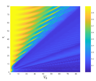
Figure 9: Surface plots of $G/G_{0}$ as a function of $V_{0}$ and $\omega$, for $E_{0}=2$, $m_{0}=0$, and (a) $L=1$ and (b) $L=0.5$.

Inside the barrier (region $II$), the Hamiltonian is given by Eq. (27),

$$H(t)~{}=~{}\hbar v~{}[k_{y}~{}\sigma^{x}~{}-~{}k^{\prime}_{x}~{}\sigma^{y}~{}+~{}V_{0}\cos(\omega t)~{}\sigma^{x}],$$ (33)

where $k^{\prime}_{x}$ denotes one of the possible values of the momentum of an electron inside the barrier. We can numerically find the Floquet operator $U$ defined in Eq. (60) and find its eigenvalues which have the form $e^{\pm i\theta_{1}T}$, where we take $\theta_{1}T$ to lie in the range $[0,\pi]$. A plot of $\theta_{1}T$ versus $k^{\prime}_{x}$ is shown in Fig. 10 for $E_{0}=2$, $k_{y}=1$, $\omega=40$, $V_{0}=10$, and $m_{0}=0$. The horizontal dotted line lies at the value $E_{0}T/\hbar\simeq 0.314$. Since the Floquet eigenvalue inside the barrier must match the eigenvalue outside (regions $I$ and $III$), the intersections of the horizontal line with the plot of $\theta_{1}T$ shows the values that $k^{\prime}_{x}$ can take. We note from the figure that the three smallest possible values of $k^{\prime}_{x}$ lie near zero and $\pm\omega/v$. We will now derive these values analytically using Floquet perturbation theory soori .

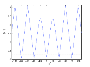
Figure 10: Plot of $\theta_{1}T$ as a function of $k^{\prime}_{x}$ obtained from a numerical evaluation of the Floquet operator $U$, for $E_{0}=2$, $k_{y}=1$, $\omega=40$, $V_{0}=10$, and $m_{0}=0$. The horizontal dotted line lies at $E_{0}T/\hbar\simeq 0.314$.

To develop the perturbation theory, we write the Hamiltonian in Eq. (33) as

$$H(t)~{}=~{}H_{0}(t)~{}+~{}V(t),$$ (34)

where $H_{0}$ is much larger than $V$. We will assume that $H_{0}(t)$ commutes with itself at different times; hence its eigenstates are time-dependent although its eigenvalues may vary with time. In our problem described by Eq. (27), we will consider two cases given by

$$H_{0} = \hbar vV_{0}\cos(\omega t)~{}\sigma^{x},$$

$$V = \hbar v~{}(k_{y}~{}\sigma^{x}~{}-~{}k^{\prime}_{x}~{}\sigma^{y}),$$ (35)

where we assume $V_{0}\gg k_{y},~{}k^{\prime}_{x}$, and

$$H_{0} = -\hbar vk^{\prime}_{x}~{}\sigma^{y},$$

$$V = \hbar v~{}[k_{y}~{}+~{}V_{0}\cos(\omega t)]~{}\sigma^{x},$$ (36)

where we assume $k^{\prime}_{x}\gg k_{y},~{}V_{0}$. We now consider the two cases in turn.

For the case given in Eq. (35), the unperturbed problem given by $i\hbar\partial\psi/\partial t=H_{0}\psi$ has solutions of the form

$$\psi_{1}(t) = \phi_{1}~{}\exp[-i(vV_{0}/\omega)~{}\sin(\omega t)],$$

$$\psi_{2}(t) = \phi_{2}~{}\exp[i(vV_{0}/\omega)~{}\sin(\omega t)],$$

$${\rm where}~{}~{}~{}\phi_{1} = \frac{1}{\sqrt{2}}~{}\begin{pmatrix}1\\ 1\end{pmatrix}~{}~{}~{}{\rm and}~{}~{}~{}\phi_{2}~{}=~{}\frac{1}{\sqrt{2}}~{}\begin{pmatrix}1\\ -1\end{pmatrix},$$ (37)

and the corresponding eigenvalues of $H_{0}(t)$ are given by $E_{1}(t)=\hbar vV_{0}\cos(\omega t)$ and $E_{2}(t)=-\hbar vV_{0}\cos(\omega t)$ respectively. Since these satisfy the condition

$$e^{(i/\hbar)\int_{0}^{T}dt~{}[E_{1}(t)-E_{2}(t)]}~{}=~{}1,$$ (38)

we have to use degenerate perturbation theory soori . Assuming that the wave function has the form

$$\psi(t)=\sum_{p=1}^{2}C_{m}(t)e^{-(i/\hbar)\int_{0}^{t}dt^{\prime}E_{m}(t^{\prime})}\phi_{m},$$ (39)

and solving for the equation $i\hbar\partial\psi/\partial t=H(t)\psi$, we obtain a differential equation for $C_{m}(t)$. Integrating from $t=0$ to $T$, we have, to first order in $V$,

$$C(T)~{}=~{}(I~{}-~{}iM)~{}C(0),$$ (40)

where $C(t)=(C_{1}(t),C_{2}(t))$ is a column, and the matrix $M$ has elements

$$M_{mn}~{}=~{}\frac{1}{\hbar}~{}\int_{0}^{T}dt~{}\psi_{m}^{\dagger}V\psi_{n}~{}e^{i\int_{0}^{t}~{}dt^{\prime}(E_{m}(t^{\prime})-E_{n}(t^{\prime}))}.$$ (41)

In our problem, $M$ is a $2\times 2$ matrix with elements

$$M_{11} = vk_{y}T,~{}~{}~{}M_{22}~{}=~{}-vk_{y}T,$$

$$M_{12} = iJ_{0}\big{(}{\frac{2V_{0}}{\omega}}\big{)}~{}vk^{\prime}_{x}T,~{}~{}~{}M_{21}~{}=~{}-~{}iJ_{0}\big{(}\frac{2V_{0}}{\omega}\big{)}~{}vk^{\prime}_{x}T.$$ (42)

Up to first order in $V$, the eigenvalues of $M$ are given by

$$\lambda_{\pm}~{}=~{}\pm~{}vT\sqrt{k_{y}^{2}~{}+~{}[J_{0}(2V_{0}/\omega)k^{\prime}_{x}]^{2}}.$$ (43)

Hence we can find eigenstates of $M$ such that

$$C_{\pm}(T)~{}=~{}e^{i\lambda_{\pm}}~{}C_{\pm}(0).$$ (44)

Since the Hamiltonian is periodic, Floquet theory implies that

$$\psi_{n}(T)~{}=~{}e^{-i\theta_{n}T}\psi_{n}(0).$$ (45)

This gives a relation between $\theta_{\pm}$ and $\lambda_{\pm}$; in our case it is

$$\theta_{\pm}~{}=~{}\pm~{}v\sqrt{k_{y}^{2}~{}+~{}[J_{0}(2V_{0}/\omega)k^{\prime}_{x}]^{2}}.$$ (46)

Since the Floquet eigenvalues in regions $I$ and $III$ given by $e^{-iE_{0}T/\hbar}$ (where $E_{0}$ is the energy of the incident electron) must be equal to the Floquet eigenvalue in region $II$ (the barrier), we obtain an expression for two of the allowed values of $k^{\prime}_{x}$, namely,

$$k^{\prime}_{x}~{}=~{}\pm~{}\frac{\sqrt{(E_{0}/\hbar v)^{2}~{}-~{}k_{y}^{2}}}{J_{0}(2V_{0}/\omega)}.$$ (47)

This gives an expression for $k^{\prime}_{x}$ of the order of $E_{0}/(\hbar v)$ which lies near zero in Fig. 10 since we have taken $E_{0}\ll\hbar\omega$ in that figure.

Eq. (47) implies that if $J_{0}(2V_{0}/\omega)=0$, there is no value of $k^{\prime}_{x}$ for which the Floquet eigenvalue in region $II$ will match the Floquet eigenvalues in regions $I$ and $III$, except for the special case $k_{y}=\pm E_{0}/(\hbar v)$ which corresponds to grazing incidence where the transmission probability is always zero. Hence, it is not possible to an electron to transmit through region $II$ if the parameters $(V_{0},\omega)$ lie on one of the straight lines where $J_{0}(2V_{0}/\omega)=0$. The first five zeros of $J_{0}(z)$ are given by $z=2.405,5.520,8.654,11.792$ and $14.931$, which give $\omega/V_{0}=0.832,0.362,0.231,0.170$ and $0.134$. We see in Fig. 11 that the conductance is indeed particularly small on the white lines whose slopes correspond to zeros of $J_{0}(2V_{0}/\omega)$.

We now turn to the case given in Eq. (36). The unperturbed problem given by $i\hbar\partial\psi/\partial t=H_{0}\psi$ has solutions of the form

$$\psi_{1}(t) = \phi_{1}~{}e^{-ivk^{\prime}_{x}t},$$

$$\psi_{2}(t) = \phi_{2}~{}e^{ivk^{\prime}_{x}t},$$

$${\rm where}~{}~{}~{}\phi_{1} = \frac{1}{\sqrt{2}}~{}\begin{pmatrix}1\\ -i\end{pmatrix}~{}~{}~{}{\rm and}~{}~{}~{}\phi_{2}~{}=~{}\frac{1}{\sqrt{2}}~{}\begin{pmatrix}1\\ i\end{pmatrix},$$ (48)

and the corresponding eigenvalues of $H_{0}$ are given by $E_{1}=k^{\prime}_{x}$ and $E_{2}=-k^{\prime}_{x}$ respectively. These do not satisfy the condition in Eq. (38) if $k^{\prime}_{x}\neq n\omega/(2v)$ for any integer value of $n$. We can then use non-degenerate perturbation theory soori . Assuming that the wave function has the form

$$\psi(t)=\sum_{p=1}^{2}C_{m}(t)e^{-(i/\hbar)\int_{0}^{t}dt^{\prime}E_{m}(t^{\prime})}\phi_{m},$$ (49)

and solving for the equation $i\hbar\partial\psi/\partial t=H(t)\psi$, we obtain the following coupled differential equations

$$\frac{dC_{1}}{dt} = e^{i2vk^{\prime}_{x}t}~{}v~{}[k_{y}~{}+~{}V_{0}\cos(\omega t)]~{}C_{2},$$

$$\frac{dC_{2}}{dt} = -~{}e^{-i2vk^{\prime}_{x}t}~{}v~{}[k_{y}~{}+~{}V_{0}\cos(\omega t)]~{}C_{1}.$$ (50)

To solve these equations, we have to choose the initial conditions $(C_{1}(0),C_{2}(0))$. To find the change in the Floquet eigenvalue $e^{-i\theta_{1}T}$ of a Floquet eigenstate which lies close to $\psi_{1}(t)$, we choose $C_{1}(0)=1$ and $C_{2}(0)$ to be small and of order $k_{y},~{}V_{0}$. Demanding that $\psi(T)=e^{-i\theta_{1}T}\psi(0)$, we discover that $\theta_{1}$ differs from $k^{\prime}_{x}T$ only at second order in the perturbation, namely,

$$\theta_{1}~{}=~{}v~{}\left[k^{\prime}_{x}~{}+~{}\frac{k_{y}^{2}}{2k^{\prime}_{x}}~{}+~{}\left(\frac{V_{0}}{2}\right)^{2}~{}\frac{1}{2k^{\prime}_{x}~{}+~{}\omega/v}~{}+~{}\left(\frac{V_{0}}{2}\right)^{2}~{}\frac{1}{2k^{\prime}_{x}~{}-~{}\omega/v}\right],$$ (51)

modulo integer multiples of $\omega$ since $\theta_{1}$ is a periodic variable with period $\omega$. A similar calculation for a Floquet eigenstate which lies close to $\psi_{2}(t)$ shows that $\theta_{2}=-\theta_{1}$. Eq. (51) shows that the second order correction is small except around the points $k^{\prime}_{x}=0$ and $\pm\omega/(2v)$.

Next, we can study what happens if $k^{\prime}_{x}=n\omega/(2v)$ where the condition in Eq. (38) is satisfied. We then have to use degenerate perturbation theory as described in Eqs. (39-41). We discover that the matrix $M$ defined in Eq. (41) is identically equal to zero if $k^{\prime}_{x}\neq 0,~{}\pm\omega/(2v)$. We can therefore use non-degenerate perturbation theory and go up to second order as in Eq. (51). We thus conclude that Eq. (51) holds for any value of $k^{\prime}_{x}$ except around 0 and $\pm\omega/(2v)$.

We now study the region around $k^{\prime}_{x}=\pm\omega/v$ where we have pairs of solutions for $\theta_{1}T=E_{0}T/\hbar$ as we see in Fig. 10. We can find an expression for the two solutions near $k^{\prime}_{x}=\omega/v$ by replacing $k^{\prime}_{x}$ by $\omega/v$ in the last three terms in Eq. (51) (which are of second order in the perturbation) but not in the first term. Eq. (51) then implies that the two possible values of $k^{\prime}_{x}$ which yield $\theta_{1}=E_{0}/\hbar$ modulo $\omega$ are given by

$$k^{\prime}_{x}~{}=~{}\frac{\omega}{v}~{}\pm~{}\frac{E_{0}}{\hbar v}~{}-~{}\frac{vk_{y}^{2}}{2\omega}~{}-~{}\frac{vV_{0}^{2}}{3\omega}.$$ (52)

Since $E_{0}\geq\hbar v|k_{y}|$, and we are working in the regime $\hbar\omega\gg E_{0}$, we can ignore the term $vk_{y}^{2}/(2\omega)$. We then get

$$k^{\prime}_{x}~{}=~{}\frac{\omega}{v}~{}\pm~{}\frac{E_{0}}{\hbar v}~{}-~{}\frac{vV_{0}^{2}}{3\omega}.$$ (53)

In problems involving transmission through a barrier, we typically find that the condition for resonances is given by $e^{ik^{\prime}_{x}L}=\pm 1$, where $k^{\prime}_{x}$ is the momentum inside the barrier (see, for instance, Ref. schwabl, ). This requires that $k^{\prime}_{x}=p\pi/L$, where $p=1,2,3,\cdots$. Since the last two terms in Eq. (53) are small, we obtain the approximate expression

$$\omega~{}=~{}\frac{\pi pv}{L}~{}\pm~{}\frac{E_{0}}{\hbar}~{}+~{}\frac{vLV_{0}^{2}}{3\pi p}.$$ (54)

This implies that in a plot of the conductance versus $(V_{0},\omega)$, the resonance regions (large conductance) will have a spacing given by $\pi v/L$ when $V_{0}=0$ and will curve up as $V_{0}^{2}$ when $V_{0}$ is increased, provided that $V_{0}/\omega$ is small. This is exactly what we see in Fig. 12 where the black and red lines are given by Eq. (54), where the second term is $\pm E_{0}/\hbar$ respectively, and the integer $p$ increases as we go up from the bottom to the top. In the figure, we see that the spacing between either the black lines or the red lines is $\pi v/L=\pi$ at $V_{0}=0$. The black and red lines go up quadratically with increasing $V_{0}$ with the correct curvatures as given in Eq. (54).

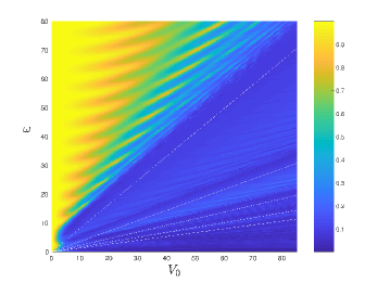
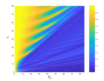
Figure 11: Surface plots of $G/G_{0}$ as a function of $V_{0}$ and $\omega$, for $E_{0}=2$, $m_{0}=0$, and (a) $L=1$ and (b) $L=0.5$. These are the same as Figs. 9 (a) and (b), but we have added some straight white lines corresponding to $J_{0}(2V_{0}/\omega)=0$; from top to bottom, these lines have slopes given by $0.832,0.362,0.231,0.170$ and $0.134$.

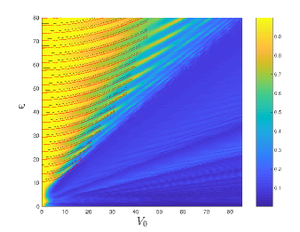
Figure 12: Surface plot of $G/G_{0}$ as a function of $V_{0}$ and $\omega$, for $E_{0}=2$, $m_{0}=0$, and $L=1$. This is the same as Fig. 9 (a), but we have added black and red lines which are given by Eq. (54), where the second term is $\pm E_{0}/\hbar$ respectively, and the integer $p$ increases as we go up from the bottom to the top.

III.1.3 Effective time-independent magnetic barrier

In this section, we will map the time-dependent system with a given set of parameter values $(m_{0},~{}V_{0},~{}\omega)$ to a time-independent system with a magnetic barrier which has only the term $m_{0}\sigma^{x}$; we do the mapping by demanding that the two systems should have the same value of the differential conductance. The procedure is as follows. On the one hand, we will calculate the conductance of the time-dependent system and find its dependence on $m_{0}$ and $\omega$, keeping $V_{0}$ fixed. On the other hand, we will calculate the conductance for the time-independent system and find its dependence on the single parameter $m_{0}$. We will then use the condition of equal conductance to find an effective value of $m_{0}$, called $m_{eff}$, of the time-independent system as a function of $\omega$ and $m_{0}$ of the time-dependent system.

We therefore first look at the time-dependent system and calculate the conductance as a function of $\omega$ for different values of $m_{0}$ and fixed $V_{0}=1.1$. This is shown in Fig. 13. Next, we consider a time-independent system with a barrier strength $m_{0}$. The Hamiltonian in region $II$ of this system is given by

$$i\hbar\dfrac{\partial\psi}{\partial t}~{}=~{}\hbar v~{}[k_{y}\sigma^{x}~{}-~{}k^{\prime}_{x}\sigma^{y}~{}+~{}m_{0}\sigma^{x}]~{}\psi.$$ (55)

The conductance of this system as a function of $m_{0}$ is shown in Fig. 14.

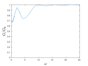
Figure 13: $G/G_{0}$ as a function of $\omega$ for $V_{0}=1.1$, $E_{0}=2$, $L=1$, and $m_{0}=0$.

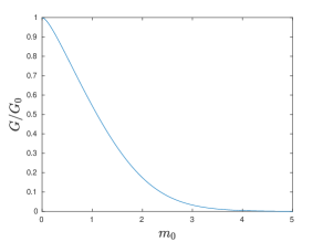
Figure 14: $G/G_{0}$ as a function of $m_{0}$ in a time-independent system with $E_{0}=2$ and $L=1$.

Finally, we can use Figs. 13 and 14 to map the time-dependent system with some values of $\omega$ and $m_{0}$ to a time-dependent system with a barrier strength $m_{eff}$, by demanding that the two systems should have the same conductance. Fig. 15 shows $m_{eff}$ as a function of $\omega$, for $V_{0}=1.1$ and $m_{0}=0$ in the time-dependent system. We have set $E_{0}=2$ in all cases. In Fig. 15 we see that $m_{eff}$ approaches a constant as $\omega$ becomes large. This can be understood using the fact that when $m_{0}$ and $V_{0}$ are fixed, the conductance of time-dependent system tends to a constant when $\omega$ becomes much larger than all the other energy scales in the problem. The reason for this is similar to the one given in Sec. II.2.5 for the case of a $\delta$-function magnetic barrier. We note from Fig. 15 that $m_{eff}$ is large for small frequencies whereas it goes to zero for large frequencies. This allows for a frequency induced control over the barrier conductance for a fixed amplitude. For large frequencies, one expects the junction to be conducting (since $m_{eff}\simeq 0$) while for small frequencies one has large $m_{eff}$ which will lead to $G\to 0$.

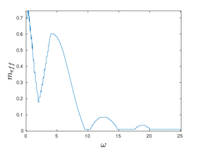
Figure 15: $m_{eff}$ of the time-independent problem as a function of $\omega$, for $V_{0}=1.1$, and $m_{0}=0$ in the time-dependent system. We have taken $E_{0}=2$ and $L=1$.

III.1.4 Conductance as a function of $E_{0}$

Finally, we study the conductance as a function of the incident energy $E_{0}$ for different values of $\omega$ and some fixed values of $m_{0}$ and $V_{0}$. We find an interesting result that there is a dip in the conductance around $E_{0}=\hbar\omega/2$; the dips are quite prominent when $\omega$ is large. This is shown in Fig. 16.

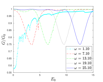
Figure 16: $G/G_{0}$ as a function of $E_{0}$ for different values of barrier strength $\omega$, for $L=1$, $m_{0}=0$ and $V_{0}=1.1$.

These dips can be understood as follows. When $E_{0}=\hbar\omega/2$, we have $E_{-1}=E_{0}-\hbar\omega=-E_{0}$, namely, the energies of the bands $n=0$ and $-1$ become equal in magnitude. We then find numerically that the maximum contribution to the conductance comes from only these two bands. Hence ignoring the contributions from all the other bands, we can proceed to study this problem analytically. To find the allowed values of $k^{\prime}_{x}$ inside the barrier, we have to solve the eigenvalue equation as in Eq. (30), but now with just two bands. The equation then takes the form

$$\begin{pmatrix}-i\hbar vk_{y}&iE_{-1}&-\frac{i\hbar vV_{0}}{2}&0\\ -iE_{-1}&i\hbar vk_{y}&0&\frac{i\hbar vV_{0}}{2}\\ -\frac{i\hbar vV_{0}}{2}&0&-i\hbar vk_{y}&iE_{0}\\ 0&\frac{i\hbar vV_{0}}{2}&-iE_{0}&i\hbar vk_{y}\end{pmatrix}\begin{pmatrix}\alpha_{-1}\\ \beta_{-1}\\ \alpha_{0}\\ \beta_{0}\end{pmatrix}~{}=~{}\hbar vk^{\prime}_{x}\begin{pmatrix}\alpha_{-1}\\ \beta_{-1}\\ \alpha_{0}\\ \beta_{0}\end{pmatrix}.$$ (56)

(We have taken $m_{0}=0$, hence $k^{\prime}_{y}=k_{y}$). We then find that the values of $k^{\prime}_{x}$ are given by

$$\hbar^{2}v^{2}k_{x}^{{}^{\prime}2}~{}=~{}\frac{1}{2}~{}\Bigl{[}~{}E_{0}^{2}+E_{-1}^{2}-\frac{\hbar^{2}v^{2}V_{0}^{2}}{2}-2\hbar^{2}v^{2}k_{y}^{2}~{}\pm~{}\sqrt{(E_{0}^{2}-E_{-1}^{2})^{2}-\hbar^{2}v^{2}V_{0}^{2}(E_{-1}-E_{0})^{2}+4\hbar^{4}v^{4}V_{0}^{2}k_{y}^{2}}\Bigr{]}.$$ (57)

Assuming that $V_{0}$ is small, we see that if $E_{0}$ is not equal to $\hbar\omega/2$, the change in $k_{x}^{{}^{\prime}2}$ is of the order of $V_{0}^{2}$, but if $E_{0}=\hbar\omega/2$, we get

$$k_{x}^{{}^{\prime}2}~{}=~{}k_{x,0}^{2}~{}\pm~{}iV_{0}k_{x,0},$$ (58)

giving a change in $k_{x}^{{}^{\prime}2}$ of the order of $V_{0}$. Thus, for $V_{0}$ small, $E_{0}=\hbar\omega/2$ gives a much larger change in $k^{\prime}_{x}$ as compared to $E_{0}\neq\hbar\omega/2$. Next, Eq. (58) implies that $k^{\prime}_{x}=k_{x,0}\pm iV_{0}/2$ has an imaginary part given by $iV_{0}/2$. Hence the wave function $e^{ik^{\prime}_{x}L}$ decays exponentially as $e^{-V_{0}L/2}$ as we go across the barrier region from $x=0$ to $L$; this reduces the transmitted particle current and hence the conductance. We can find the width of the region of low conductance around $E_{0}=\hbar\omega/2$ by using Eq. (57) to determine when $k^{\prime}_{x}$ becomes complex. We find that this happens when

$$|E_{0}~{}-~{}\frac{\hbar\omega}{2}|~{}<~{}\dfrac{\hbar vV_{0}}{2}~{}\sqrt{1~{}-~{}\frac{4v^{2}k_{y}^{2}}{\omega^{2}}},$$ (59)

which is proportional to $V_{0}$. Thus the width of the dip in the conductance is expected to be proportional to $V_{0}$ while the magnitude of the dip (which is related to the transmission probability) should be proportional to $e^{-V_{0}L}$ since the transmission amplitude is proportional to $e^{-V_{0}L/2}$. If we hold $V_{0}L$ fixed and vary $L$, the magnitude of the dip should remain the same but the width should be proportional to $V_{0}$ and therefore inversely proportional to $L$. This agrees with the plot shown in Fig. 17 where we have plotted the differential conductance as a function of $E_{0}$ for two values of $L$, with $m_{0}=1$, $\omega=25.1$, and $V_{0}L=2.3$. Thus by varying $E_{0}$, $\omega$ and $V_{0}$, we can tune the conductance and achieve a switching behavior close to $E_{0}=\hbar\omega/2$.

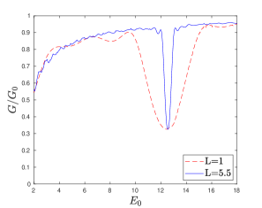
Figure 17: $G/G_{0}$ as a function of $E_{0}$ for $m_{0}=1$, $\omega=25.1$, and $L=1$ and $5.5$, keeping $V_{0}L=2.3$ fixed.

IV Discussion

In this work, we have studied transport across a magnetic barrier placed on the top surface of a three-dimensional TI, where the barrier strength varies sinusoidally with time in addition to having a constant term. Such a situation arises if a ferromagnetic strip is placed on top of the TI surface and a periodically driven magnetic field is applied to the ferromagnet; then the magnetization of the ferromagnet would oscillate in time. If the magnetization points along the $\hat{x}$ direction and has a Zeeman coupling to the spin of the electrons on the TI surface, it would lead to the time-dependent Hamiltonian that we have studied in this paper. Alternatively, the ferromagnetic strip could have a time-independent magnetization along the $\hat{x}$ direction, and a electromagnetic field (which is linearly polarized along the $\hat{y}$ direction) can be applied to the same region of the surface of the TI. The vector potential of the electromagnetic field would point along the $\hat{y}$ direction and vary periodically in time; this would lead to the same time-dependent Hamiltonian.

We have studied two kinds of time-dependent magnetic barriers: a $\delta$-function barrier and a barrier which has a finite width $L$. The $\delta$-function barrier leads to a discontinuity of the wave function of a specific kind. For the finite width barrier, we have to match the wave function at the two edges of the barrier. In both cases, we have to take into account a large number of Floquet bands. We consider what happens when an electron is incident on the barrier from the left with an energy $E_{0}$ and an angle of incidence $\theta$. We numerically calculate the transmitted current as a function of $\theta$; integrating this over $\theta$ gives the differential conductance $G$ when a voltage equal to $E_{0}$ is applied to the leads. We have studied these quantities as a function of $E_{0}$, the driving frequency $\omega$, and the constant $m_{0}$ and the oscillation amplitude $V_{0}$ of the barrier strength.

Our main results are as follows. For the transmitted current, we find kinks at certain values of $\theta$. These arise because the momentum in the direction of propagation changes from a real to a complex value in some side band at those values of $\theta$; the corresponding wave function changes from a plain wave to an exponentially decaying wave which then leads to a drop in the transmitted current. For small values of $\omega$ (the adiabatic limit), one can approximate the results well by averaging over a sequence of time-independent values of the barrier strength. We then find that there are peaks in the conductance when $m_{0}$ is equal to $\pm V_{0}$ since the barrier strength stays close to zero for long periods of time. For large values of $\omega$, we find numerically that the transmission is dominated by three Floquet bands; the central band $n=0$ and the first two side bands $n=\pm 1$. This allows us to calculate the conductance more easily. We have shown that the time-dependent barrier problem can be mapped to a time-independent magnetic barrier with an effective strength $m_{eff}$ whose value depends on the driving parameters. Thus the conductance of the driven system can be effectively characterized by a static parameter.

Next, we have analyzed surface plots of the conductance as a function of $V_{0}$ and $m_{0}$, for different values of $\omega$. When $\omega$ and $V_{0}$ are large compared to $E_{0}$, and $m_{0}$ is small, we find that the conductance has peaks at a discrete set of values of $V_{0}$. To understand this better, we have made a detailed study of the conductance as a function of $V_{0}$ and $\omega$, keeping $E_{0}$ and $L$ fixed and taking $m_{0}=0$. We find that the behavior of $G$ is quite different depending on whether $\omega/V_{0}$ lies above or below a value equal to $0.83$ (this is related to the first zero of the Bessel function $J_{0}(z)$). When $\omega/V_{0}\gtrsim 0.83$, the conductance is large along certain curves in the $(V_{0},\omega)$ plane; these curves correspond to resonances, and their spacing is proportional to $1/L$. When $\omega/V_{0}\lesssim 0.83$, the conductance is generally small; however it is particularly small along certain straight lines whose slopes are related to the successive zeros of $J_{0}(z)$. We present a Floquet perturbation theory which can explain both the resonances and lines of very small conductances. We have then studied the conductance as a function of the incident energy $E_{0}$. We find that this shows a prominent dip when $E_{0}$ is close to $\hbar\omega/2$ when these quantities are much larger than $m_{0}$ and $V_{0}$. We can understand this as follows. When $E_{0}=\hbar\omega/2$, the energy in one of the side bands, $E_{-1}$, becomes equal in magnitude to $E_{0}$. We then find numerically that the conductance is dominated by only the two bands, $n=0$ and $-1$. This allows us to analytically estimate the width and magnitude of the conductance dips. We find that the width is proportional to $V_{0}$, in agreement with the numerical results.

Our results can be experimentally tested as follows. As mentioned in Sec. II.2, an energy of $0.01$ eV corresponds to a frequency scale of about 15 THz. This gives an estimate of the required frequency $\omega$ if electromagnetic radiation is used to produce the time-dependent magnetic barrier. The strength $V_{0}$ of the magnetic barrier is proportional to the vector potential $\cal A$; this is related to the electric field $\cal E$ (as ${\cal E}=\omega{\cal A}$) and hence to the intensity of the radiation. Our most important result is that when $\omega$ is much larger than the energy $E_{0}$ of the electrons ($\omega\gg E_{0}/\hbar$), the conductance across the barrier has a striking dependence on $V_{0}$ and $\omega$ as indicated in Fig. 9. For instance, increasing the intensity of the radiation keeping the frequency fixed or decreasing the frequency keeping the intensity fixed should reduce the conductance sharply as we cross a line in the $(V_{0},\omega)$ plane. Further, the conductance shows resonance-like features when the conductance is large, and these features depend sensitively on the width of the barrier. Another interesting feature appears when $\omega$ is of the order of $E_{0}/\hbar$; namely, there is a prominent dip in the conductance when $\omega$ crosses $2E_{0}/\hbar$, and this dip becomes sharper as the barrier length is increased.

Finally, we have used a semiclassical approach to study this problem in the limit where the spin of the particle is very large instead of being 1/2. This allows us to use classical equations of motion to study the motion of the particle in the presence of a time-dependent magnetic barrier, assuming that at time $t=0$ it is incident on the left edge of the barrier at a normal angle of incidence. We find that although the motion of the particle can be quite complicated inside the barrier, it eventually escapes either to the left or to the right of the barrier. To connect this with the study of spin-1/2 electrons done in the earlier sections, we interpret escaping to the left (right) as reflection (transmission) and therefore as small and large conductances respectively. With this interpretation, we find that the behaviors of the system as a function of the barrier parameters $\omega$, $m_{0}$ and $V_{0}$ show a qualitative match between spin-1/2 and the large spin limit.

We have not considered the effects of disorder and have only studied ballistic transport in this work. If there is strong disorder, the mean free path of the electrons becomes less than the width of the magnetic barrier, and the effect of disorder would have to be considered. This would be an interesting problem to study in the future. However, our results should hold with minor modifications in the weak disordered limit fogler . Moreover, we have not addressed the effects of interactions between the Dirac electrons which may lead to heating effects, specially at low drive frequencies. A detailed study of this problem is left as a subject of future study.

Acknowledgments

D.S. thanks Amit Agarwal, Sankalpa Ghosh and Puja Mondal for stimulating discussions. D.S. also thanks DST, India for Project No. SR/S2/JCB-44/2010 for financial support.

Appendix A Basics of Floquet theory

In this section we briefly recapitulate Floquet theory bukov ; mikami . Given a Hamiltonian which varies periodically in time with a time period $T=2\pi/\omega$, namely, $H(t+T)=H(t)$, we want to find the solutions of the equation $i\hbar\partial\psi(t)/\partial t=H(t)\psi(t)$. To this end, we define the Floquet operator which time evolves the system through one time period,

$$U~{}=~{}{\cal T}~{}\exp[-~{}\frac{i}{\hbar}~{}\int_{0}^{T}~{}dtH(t)],$$ (60)

where $\cal T$ denotes time-ordering. Thus, $\psi(T)=U\psi(0)$. Since $U$ is a unitary operator, its eigenvalues must be phases; denoting the $n$-th eigenvalue and eigenstate as $e^{-i\theta_{n}T}$ and $\psi_{n}(0)$, we have

$$U\psi_{n}(0)~{}=~{}e^{-i\theta_{n}T}~{}\psi_{n}(0).$$ (61)

We can find $\theta_{n}$ and $\psi_{n}(0)$ as follows. Eq. (61) implies that $\psi_{n}(T)=e^{-i\theta_{n}T}\psi_{n}(0)$. We can therefore write

$$\psi_{n}(t)~{}=~{}e^{-i\theta_{n}t}~{}\sum_{m=-\infty}^{\infty}~{}e^{-im\omega t}\psi_{n,m},$$ (62)

so that $\psi_{n}(0)=\sum_{m=-\infty}^{\infty}\psi_{n,m}$. Next, the periodicity of the Hamiltonian in time means that we can write

$$H(t)~{}=~{}\sum_{m=-\infty}^{\infty}~{}H_{m}~{}e^{-im\omega t},$$ (63)

where $H_{m}$ is given by $H_{m}=(1/T)\int_{0}^{T}dtH(t)e^{im\omega t}$. The equation $i\hbar\partial\psi(t)/\partial t=H(t)\psi(t)$ then leads to the infinite set of coupled time-independent equations,

$$\sum_{p=-\infty}^{\infty}~{}(H_{m-p}~{}-~{}m\hbar\omega~{}\delta_{m,p})~{}\psi_{n,p}~{}=~{}\hbar\theta_{n}~{}\psi_{n,m}.$$ (64)

where $m$ runs over all values from $-\infty$ to $\infty$. We can solve these equations to find $\theta_{n}$ and $\psi_{n}(0)$; a numerical solution typically requires an upper and a lower cut-off for the values of $p$.

Appendix B Semiclassical approach

In the earlier sections, we have studied the transmission of spin-1/2 electrons through a time-dependent magnetic barrier. It may be instructive, however, to look at the more general problem of the transmission of a spin-$S$ particle whose spin angular momentum operators $\vec{S}$ satisfy ${\vec{S}}^{2}=S(S+1)\hbar^{2}$. In particular, we will study the semiclassical limit $S\to\infty$ and see if this can give a qualitative understanding of some of the phenomena that we have discovered for the spin-1/2 case.

In this section, we investigate the semiclassical dynamics of a charged particle with spin maiti which is moving in two dimensions in the presence of a time-dependent magnetic barrier with a finite width. The dynamics involves two two-dimensional vectors, namely, the position of the particle ${\vec{r}}=(x,y)$ and the canonically conjugate momentum ${\vec{p}}=(p_{x},p_{y})$. In addition, the dynamics also involves a three-dimensional unit vector ${\vec{n}}=(n_{1},n_{2},n_{3})$ which is related to the spin vector $\vec{S}$ as ${\vec{n}}={\vec{S}}/(S\hbar)$; in the limit $S\to\infty$, $\vec{n}$ becomes a unit vector. For convenience, we will denote $M=S\hbar$.

Classically, the different dynamical variables describing the particle satisfy the following Poisson bracket relations

$$\{r_{i},p_{j}\}_{PB}~{}=~{}\delta_{ij}~{}~{}~{}{\rm and}~{}~{}~{}\{n_{i},n_{j}\}_{PB}~{}=~{}\frac{1}{M}~{}\sum_{k=x,y,z}\epsilon_{ijk}~{}n_{k},$$ (65)

where $\epsilon_{ijk}$ is the totally antisymmetric tensor with $\epsilon_{123}=1$. All other Poisson brackets such as $\{r_{i},n_{j}\}$ and $\{p_{i},n_{j}\}$ vanish. We now consider a Hamiltonian of the form maiti

$$H = v\vec{n}\cdot\vec{\Pi}~{}+~{}q\phi,$$

$${\vec{\Pi}} = {\vec{p}}~{}-~{}q{\vec{A}},$$ (66)

where $\vec{A}$ is the vector potential, and $\phi$ is the electrostatic potential. [We note that in two dimensions, the electric field ${\vec{E}}=-{\vec{\nabla}}\phi-\partial{\vec{A}}/{\partial t}$ has two components and the magnetic field $B=\partial A_{y}/\partial x-\partial A_{x}/\partial y$ has one component]. Using Eq. (65) we find that $\{\Pi_{x},\Pi_{y}\}_{PB}=B$. The Hamiltonian that we have studied earlier, given in Eq. (27), has the form $v{\vec{\sigma}}\times{\vec{\Pi}}$ while the Hamiltonian given in Eq. (66) has the form $v\vec{n}\cdot\vec{\Pi}$. The two are related by first rotating by $\pi/2$ which transforms $\sigma^{x}\to\sigma^{y}$ and $\sigma^{y}\to-\sigma^{x}$, and then going from spin-1/2 to the large spin limit.

Now, the classical equations of motion of a dynamical variable $\cal O$ is given by

$$\frac{d{\cal O}}{dt}~{}=~{}\frac{\partial{\cal O}}{\partial t}~{}-~{}\{H,{\cal O}\}_{PB}.$$ (67)

Using Eqs. (65), we obtain the following equations

$$\dot{x} = vn_{1},~{}~{}~{}~{}~{}~{}\dot{y}~{}=~{}vn_{2},$$

$$\dot{\Pi}_{x} = q~{}[E_{x}~{}+~{}vn_{2}B],~{}~{}~{}~{}~{}~{}\dot{\Pi}_{y}~{}=~{}q~{}[E_{y}~{}-~{}vn_{1}B],$$

$$\dot{n}_{1} = \frac{v}{M}~{}n_{3}\Pi_{y},~{}~{}~{}~{}~{}~{}\dot{n}_{2}~{}=~{}-~{}\frac{v}{M}~{}n_{3}\Pi_{x},~{}~{}~{}~{}~{}~{}\dot{n}_{3}~{}=~{}\frac{v}{M}~{}(n_{2}\Pi_{x}~{}-~{}n_{1}\Pi_{y}).$$ (68)

Note that these equations preserve the constraint ${\vec{n}}^{2}=1$.

Before proceeding further, we present a simple case of Eqs. (68). In the absence of electromagnetic fields, i.e., for a free particle, we find that Eqs. (68) are invariant under rotations in the $x-y$ plane. We then find that after a suitable rotation, the solution of the equations can be written as

$$\Pi_{x} = p,~{}~{}~{}~{}~{}~{}\Pi_{y}~{}=~{}0,$$

$$n_{1} = \mu,~{}~{}~{}~{}~{}~{}n_{2}~{}=~{}\sqrt{1~{}-~{}\mu^{2}}~{}\cos(\frac{vpt}{M}~{}+~{}\alpha),~{}~{}~{}~{}~{}~{}n_{3}~{}=~{}\sqrt{1~{}-~{}\mu^{2}}~{}\sin(\frac{vpt}{M}~{}+~{}\alpha),$$

$$x = v\mu t~{}+~{}x_{0},~{}~{}~{}~{}~{}~{}y~{}=~{}\frac{M\sqrt{1~{}-~{}\mu^{2}}}{p}~{}\sin(\frac{vpt}{M}~{}+~{}\alpha)~{}+~{}y_{0},$$ (69)

where $p,~{}\mu,\alpha,x_{0}$ and $y_{0}$ are constants, and $\mu$ must lie in the range $[-1,1]$. Note that the particle moves with constant velocity $v\mu$ in one direction ($x$) but oscillates in the transverse direction ($y$). The velocity $v\mu$ can take any value from $+v$ to $-v$. This agrees with the fact that if a spin-$S$ particle has a Hamiltonian of the form $H=(v/\hbar S){\vec{S}}\cdot{\vec{p}}$, the group velocity is given by $v_{g}=(v/\hbar S){\vec{S}}\cdot{\hat{p}}$. Then the fact that eigenvalues of $(1/\hbar){\vec{S}}\cdot{\hat{p}}$ are quantized as $S,~{}S-1,~{}\cdots,~{}-S$, implies that $v_{g}$ can take $2S+1$ values in the range $[-v,v]$. In the limit $S\to\infty$, $v_{g}$ can take all values in the above range.

Returning to our problem described by Eq. (27), $\phi$ and $A_{x}$ are equal to zero, while the term multiplying $v\sigma^{x}$ in the barrier region is equal to $\hbar k_{y}+\hbar\{m_{0}+V_{0}\cos(\omega t)\}$. To identify this with $\Pi_{y}=p_{y}-qA_{y}$, we must take

$$qA_{y}~{}=~{}-~{}\hbar\{m_{0}+V_{0}\cos(\omega t)\}~{}~{}~{}{\rm for}~{}~{}~{}0<x<L,$$ (70)

and zero for other values of $x$. However, such a step function form for $A_{y}(x,t)$ would mean that the magnetic field $B$ would blow up as a $\delta$-function at $x=0$ and $L$. We will therefore approximate $A_{y}$ to have the continuous and piecewise linear form

$$qA_{y}(x,t) = 0\quad{\rm for}~{}~{}~{}x~{}<~{}0,$$ (71)

$$= \dfrac{x}{\delta}~{}\{m_{0}~{}+~{}V_{0}\cos(\omega t)\}\quad{\rm for}~{}~{}~{}0~{}<~{}x~{}<~{}\delta,$$

$$= m_{0}~{}+~{}V_{0}\cos(\omega t)\quad{\rm for}~{}~{}~{}\delta~{}<~{}x~{}<~{}L~{}-~{}\delta,$$

$$= \dfrac{L~{}-~{}x}{\delta}~{}\{m_{0}+V_{0}\cos(\omega t)\}\quad{\rm for}~{}~{}~{}L~{}-~{}\delta~{}<~{}x~{}<~{}L,$$

$$= 0\quad{\rm for}~{}~{}~{}x~{}>~{}L,$$

where $\delta$ is a small distance ($\delta\ll L$) over which $A_{y}$ changes between zero and the value that it has inside the barrier. We note that the parameters $m_{0},~{}V_{0}$ in the above equations are not identical to the same parameters in Eq. (27); they differ by a factor of $\hbar$.

We can now study the time evolution given by Eqs. (68), where

$$qE_{x}~{}=~{}0,~{}~{}~{}~{}qE_{y}~{}=~{}-~{}q~{}\partial A_{y}/\partial t,~{}~{}~{}~{}qB~{}=~{}q~{}\partial A_{y}/\partial x,$$ (72)

and $qA_{y}$ is given in Eq. (71). We have to choose some initial conditions at time $t=0$. We will assume that the particle comes in from $x=-\infty$ with an energy $E>0$ and arrives at $x=0,~{}y=0$ at a normal angle of incidence. Hence $x(0)=0$ (i.e., the left edge of the barrier), $y(0)=0$, while $\Pi_{x}=p_{x}=E/v$ and $\Pi_{y}=p_{y}-qA_{y}=0$ at $t=0$. Finally, the spin-momentum locking implied by the Hamiltonian in Eq. (66) implies that since $\Pi_{x}(0)>0$ and $\Pi_{y}(0)=0$, we must take choose the components of the unit vector $\vec{n}$ as $n_{1}(0)=1$ and $n_{2}(0)=n_{3}(0)=0$. To summarize, the initial conditions are

$$x(0)~{}=~{}0,~{}~{}~{}~{}~{}~{}y(0)~{}=~{}0,~{}~{}~{}~{}~{}~{}\Pi_{x}(0)~{}=~{}\frac{E}{v},~{}~{}~{}~{}~{}~{}\Pi_{y}(0)~{}=~{}0,~{}~{}~{}~{}~{}~{}n_{1}(0)~{}=~{}1,~{}~{}~{}~{}~{}~{}n_{2}(0)~{}=~{}0,~{}~{}~{}~{}~{}~{}n_{3}(0)~{}=~{}0.$$ (73)

We can now use Eqs. (68) to numerically find how the different dynamical variables change with time. Since we are specifically interested in transmission through the barrier, we will concentrate on the variable $x$.

Figures 18 and 19 show $x$ as a function of $t$ for different values of $\omega$, $m_{0}$ and $V_{0}$. We have taken $E=2$ and $v=1$ in Eq. (73) and the barrier width $L=1$ and $\delta=0.1$ in appropriate units. In these figures, we see that depending on the various parameters, the particle may have a complicated trajectory while it is inside the barrier region ($0<x<L$), but eventually it always escapes either to the left ($x<0$) with constant negative velocity or to the right ($x>L$) with a constant positive velocity. In order to compare with the results obtained in the earlier sections, we can interpret escape to the left as reflection (hence zero or small conductance) and to the right as transmission (large conductance).

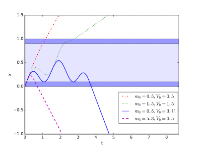
Figure 18: $x$ as a function of $t$ for $\omega=0.01$ and different values of $m_{0}$ and $V_{0}$

In Fig. 18, we see that for small and intermediate equal values of $m_{0}$ and $V_{0}$ (dash dot red and dotted green lines), there is transmission which maps to the $m_{0}-V_{0}$ plane in Fig. 8 (a). But as we increase $m_{0}$ keeping $V_{0}$ fixed, or increase $V_{0}$ keeping $m_{0}$ fixed, we see in Fig. 18 (solid blue and dashed magenta lines) that there is reflection. This maps to regions in Fig. 18, where there is no conductance. Also in Fig. 18 (solid blue line), where we have fine tuned the value of $V_{0}$, we see that the particle remains in the barrier region for a relatively longer time.

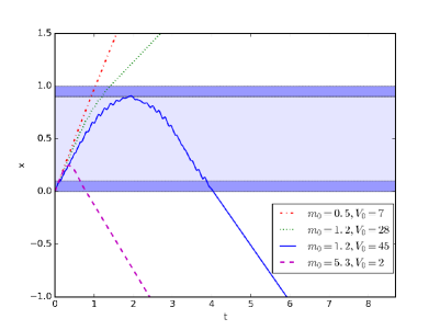
Figure 19: $x$ as a function of $t$ for $\omega=40.1$ and different values of $m_{0}$ and $V_{0}$.

In Fig. 19 we see that the value of $V_{0}=41.8$ is a cut-off, below which there is transmission and above which there is reflection. For small $m_{0}$, a comparison of Figs. 18 and 19 shows that as $\omega$ is increased, the value of $V_{0}$ beyond which there is reflection increases. This maps qualitatively to the surface plot in Fig. 8 (c) where we see that for larger $\omega$, the value of $V_{0}$ up to which there is large conductance increases. Although the cut-off values of $V_{0}$ do not match between the surface plots and the semiclassical analysis, we see that there is a qualitative mapping between the two as a function of $\omega$.

References

- (1)
- (2) M. Z. Hasan and C. L. Kane, Rev. Mod. Phys. 82, 3045 (2010).
- (3) X.-L. Qi and S.-C. Zhang, Rev. Mod. Phys. 83, 1057 (2011).
- (4) M. Brahlek, N. Koirala, M. Salehi, N. Bansal, and S. Oh, Phys. Rev. Lett. 113, 026801 (2014).
- (5) S. K. Kushwaha, I. Pletikosić, T. Liang, A. Gyenis, S. H. Lapidus, Y. Tian, H. Zhao, K. S. Burch, H. Ji, A. V. Fedorov, A. Yazdani, N. P. Ong, T. Valla, and R. J. Cava, Nature Communications 7, 11456 (2016).
- (6) T. Yokoyama, Y. Tanaka, and N. Nagaosa, Phys. Rev. B 81, 121401 (R) (2010).
- (7) S. Mondal, D. Sen, K. Sengupta, and R. Shankar, Phys. Rev. Lett. 104, 046403 (2010), and Phys. Rev. B 82, 045120 (2010).
- (8) M. S. Rudner, N. H. Lindner, E. Berg, and M. Levin, Phys. Rev. X 3, 031005 (2013).
- (9) F. Nathan and M. S. Rudner, New J. Phys. 17, 125014 (2015).
- (10) J. Cayssol, B. Dóra, F. Simon, and R. Moessner, Phys. Status Solidi RRL 7, 101 (2013).
- (11) N. Goldman and J. Dalibard, Phys. Rev. X 4, 031027 (2014).
- (12) A. Eckardt and E. Anisimovas, New J. Phys. 17, 093039 (2015).
- (13) M. Bukov, L. D’Alessio, and A. Polkovnikov, Advances in Physics 64, 139 (2015).
- (14) T. Mikami, S. Kitamura, K. Yasuda, N. Tsuji, T. Oka, and H. Aoki, Phys. Rev. B 93, 144307 (2016).
- (15) A. Das, Phys. Rev. B 82, 172402 (2010).
- (16) S. Bhattacharyya, A. Das, and S. Dasgupta, Phys. Rev. B 86, 054410 (2012).
- (17) S. S. Hegde, H. Katiyar, T. S. Mahesh, and A. Das, Phys. Rev. B 90, 174407 (2014).
- (18) S. Mondal, D. Pekker, and K. Sengupta, EPL 100, 60007 (2012).
- (19) T. Nag, S. Roy, A. Dutta and D. Sen, Phys. Rev. B 89, 165425 (2014).
- (20) T. Nag, D. Sen and A. Dutta, Phys. Rev. A 91, 063607 (2015).
- (21) A. Agarwala, U. Bhattacharya, A. Dutta and D. Sen, Phys. Rev. B 93, 174301 (2016).
- (22) T. Oka and H. Aoki, Phys. Rev. B79, 081406(R) (2009).
- (23) J.-I. Inoue and A. Tanaka, Phys. Rev. Lett. 105, 017401 (2010).
- (24) T. Kitagawa, T. Oka, A. Brataas, L. Fu, and E. Demler, Phys. Rev. B 84, 235108 (2011).
- (25) T. Kitagawa, E. Berg, M. Rudner, and E. Demler, Phys. Rev. B 82, 235114 (2010).
- (26) Z. Gu, H. A. Fertig, D. P. Arovas, and A. Auerbach, Phys. Rev. Lett. 107, 216601 (2011).
- (27) N. H. Lindner, G. Refael, and V. Galitski, Nature Phys. 7, 490 (2011).
- (28) E. Suarez Morell and L. E. F. Foa Torres, Phys. Rev. B 86, 125449 (2012).
- (29) Y. T. Katan and D. Podolsky, Phys. Rev. Lett. 110, 016802 (2013).
- (30) P. Delplace, A. Gomez-Leon and G. Platero, Phys. Rev. B 88, 245422 (2013).
- (31) Q.-J. Tong, J.-H. An, J. Gong, H.-G. Luo, and C. H. Oh, Phys. Rev. B 87, 201109(R) (2013).
- (32) M. Thakurathi, A. A. Patel, D. Sen, and A. Dutta, Phys. Rev. B 88, 155133 (2013).
- (33) M. Thakurathi, K. Sengupta, and D. Sen, Phys. Rev. B 89, 235434 (2014).
- (34) G. Usaj, P. M. Perez-Piskunow, L. E. F. Foa Torres, and C. A. Balseiro, Phys. Rev. B 90, 115423 (2014).
- (35) A. Kundu, H. A. Fertig, and B. Seradjeh, Phys. Rev. Lett. 113, 236803 (2014).
- (36) D. Carpentier, P. Delplace, M. Fruchart, and K. Gawedzki, Phys. Rev. Lett. 114, 106806 (2015).
- (37) L. D’Alessio and M. Rigol, Nature Communications 6, 8336 (2015).
- (38) T.-S. Xiong, J. Gong, and J.-H. An, Phys. Rev. B 93, 184306 (2016).
- (39) M. Thakurathi, D. Loss, and J. Klinovaja. Phys. Rev. B 95, 155407 (2017).
- (40) B. Mukherjee, A. Sen, D. Sen, and K. Sengupta, Phys. Rev. B 94, 155122 (2016).
- (41) B. Mukherjee, P. Mohan, D. Sen, and K. Sengupta, Phys. Rev. B 97, 205415 (2018).
- (42) L. Zhou and J. Gong, Phys. Rev. B 97, 245430 (2018).
- (43) A. Kundu and B. Seradjeh, Phys. Rev. Lett. 111, 136402 (2013).
- (44) A. Agarwala and D. Sen, Phys. Rev. B 96, 104309 (2017).
- (45) P. Mondal, S. Ghosh, and M. Sharma, J. Phys. Condens. Matter 31, 495001 (2019).
- (46) M. Abramowitz and I. A. Stegun, Handbook of Mathematical Functions (Dover, New York, 1972).
- (47) M. Moskalets and M. Büttiker, Phys. Rev. B 66, 205320 (2002).
- (48) A. Agarwal and D. Sen, Phys. Rev. B 76, 235316 (2007).
- (49) A. Udupa, K. Sengupta, and D. Sen, Phys. Rev. B 98, 205413 (2018).
- (50) A. Soori and D. Sen, Phys. Rev. B 82, 115432 (2010).
- (51) F. Schwabl, Quantum Mechanics (Springer, Berlin, 1995).
- (52) M. Maiti and R. Shankar, J. Phys. A 45, 185307 (2012).
- (53) M. M. Fogler, F. Guinea, and M. I. Katsnelson, Phys. Rev. Lett. 101, 226804 (2008).