A Semi-Parametric Estimation Method for the Quantile Spectrum with an Application to Earthquake Classification Using Convolutional Neural Network

Abstract

In this paper, a new estimation method is introduced for the quantile spectrum, which uses a parametric form of the autoregressive (AR) spectrum coupled with nonparametric smoothing. The method begins with quantile periodograms which are constructed by trigonometric quantile regression at different quantile levels, to represent the serial dependence of time series at various quantiles. At each quantile level, we approximate the quantile spectrum by a function in the form of an ordinary AR spectrum. In this model, we first compute what we call the quantile autocovariance function (QACF) by the inverse Fourier transformation of the quantile periodogram at each quantile level. Then, we solve the Yule-Walker equations formed by the QACF to obtain the quantile partial autocorrelation function (QPACF) and the scale parameter. Finally, we smooth QPACF and the scale parameter across the quantile levels using a nonparametric smoother, convert the smoothed QPACF to AR coefficients, and obtain the AR spectral density function. Numerical results show that the proposed method outperforms other conventional smoothing techniques. We take advantage of the two-dimensional property of the estimators and train a convolutional neural network (CNN) to classify smoothed quantile periodogram of earthquake data and achieve a higher accuracy than a similar classifier using ordinary periodograms.

Key Words: Quantile periodogram; Autoregressive approximation; Convolutional neural network; Earthquake data classification

1 Introduction

Motivated by the least-squares interpretation of the ordinary periodogram, Li, 2012b proposed the quantile periodogram based on trigonometric quantile regression. Similarly to the behavior of the ordinary spectrum and periodogram (Brockwell and Davis,, 1984), the quantile periodogram has an asymptotic exponential distribution but the mean function, called the quantile spectrum, is a scaled version of the ordinary spectrum of the level-crossing process. Related works include Hagemann, (2013), Li, (2013), Dette et al., (2015) Lim and Oh, (2016), Birr et al., (2017, 2019), and Baruník and Kley, (2019).

The quantile periodogram was inspired by the quantile regression (Koenker,, 2005), which examines the conditional quantiles and, thus, provides a richer view of the data than the traditional least-squares regression. Just as the ordinary periodogram can be obtained by applying least squares regression to the trigonometric regressor, the quantile periodogram is computed by applying quantile regression instead of least squares regression. Since quantile regression is known for its robustness against outliers and heavy-tailed noise, quantile periodograms are also endowed with these properties. Li, 2012a used the quantile periodogram to detect and estimate hidden periodicity from noisy observations when the noise distribution was asymmetric with a heavy tail on one side, while ordinary periodograms are less effective in handling such noise. Li, (2014) applied the quantile periodogram to Dow Jones Industrial Average and showed the advantages of quantile periodograms when handling time-dependent variance.

In traditional spectral analysis, the ordinary periodogram needs to be smoothed to serve as an estimator of the underlying ordinary (or power) spectrum. Many methods have been proposed to do so. One classical method is to apply a nonparametric smoother to the periodogram across frequencies. Shumway and Stoffer, (2016) discussed several periodogram smoothing techniques include moving-average smoothing. Wahba, (1980) developed the optimally smoothed spline (OSS) estimator, and the smoothing parameter is selected to minimize the expected integrated mean square error. The span selection is an important issue in periodogram smoothing. The unbiased risk estimator is used to produce the span selector in Lee, (1997), and the selector does not require strong conditions on the spectral density function. Another popular method for spectral density estimation is based on likelihood. Capon, (1983) used the maximum-likelihood filter to produce the minimum-variance unbiased estimator of the spectral density function. Chow and Grenander, (1985) proposed a sieve for the estimation of the spectral density of a Gaussian stationary stochastic process using likelihood, and compared to standard periodogram-based estimate, the proposed method aims at exploiting the full Gaussian nature of the process. The well-known Whittle likelihood was developed for time series analysis in Whittle, (1953, 1954), and an approximation to the likelihood is constructed from the spectrum and periodogram. In Pawitan and O’Sullivan, (1994), the spectral density function is estimated by the penalized Whittle likelihood. For parametric estimation methods, the autoregressive (AR) spectral approximation is discussed in Shumway and Stoffer, (2016). Chan and Langford, (1982) and Friedlander and Porat, (1984) used the Yule-Walker method to estimate the parameters.

Similar to the ordinary periodogram, the quantile periodogram is also very noisy at each quantile level. To estimate the copula rank-based quantile spectrum, Zhang, (2019) produced an automatically smoothed estimator for the copula spectral density kernel (CSDK), along with samples from the posterior distributions of the parameters via a Hamiltonian Monte Carlo (HMC) step. Hagemann, (2013) applied the Parzen, (1957) class of kernel spectral density estimators to the quantile periodogram and characterized the asymptotic properties of the quantile and smoothed quantile periodograms. Dette et al., (2015) showed that the quantile spectrum can be estimated consistently by a window smoother of the quantile periodogram.

The ordinary spectrum is a critical feature of Gaussian time series, and it is often used to classify or cluster time series. For example, Orhan et al., (2011) introduced a classifier based on multilayer perceptron neural network (MLPNN) as a diagnostic-decision support mechanism in epilepsy treatment. Maadooliat et al., (2018) employed ordinary spectral density functions for electroencephalogram (EEG) data clustering. The quantile spectrum contains information at both the frequency levels and the quantile levels. Due to the additional information it provides compared to the ordinary periodogram, the quantile periodogram is expected to produce better classification and clustering results. The two-dimensional (2D) nature of the quantile spectrum offers opportunities to apply image-based techniques. The convolutional neural network (CNN) is an effective and popular technique for 2D image classification. For example, Krizhevsky et al., (2012) trained a large, deep CNN to classify 1.3 million high-resolution images in the LSVRC-2010 ImageNet training set. For accurate classification, a good estimation of the quantile spectrum is crucial. The quality of the estimator directly affects the classification performance.

Motivated by the function approximation capability of the autoregressive (AR) spectrum (Shumway and Stoffer,, 2011), we propose a new method that uses the parametric form of the AR spectrum to approximate the quantile spectrum at each quantile level. The novelty of our approach is threefold. First, at each quantile level, we approximate the quantile spectrum by the ordinary AR spectral density derived from what we call the quantile autocovariance function as the Fourier transform of the quantile periodogram, where the order of the AR model is automatically selected by the AIC. Furthermore, we apply nonparametric smoothing techniques with respect to the quantile levels for the AR orders as well as the AR coefficients, where the latter is carried out in the partial autocorrelation domain to ensure the causality of the approximating AR spectrum. Therefore, the proposed method ensures not only the smoothness with respect to the frequencies but also the smoothness with respect to the quantile levels. Finally, we treat the smoothed quantile periodograms as images and apply image classification techniques to classify time series. For the case study, we employ the proposed quantile spectral estimation technique, coupled with a CNN classifier, to classify a set of time series for earthquakes. The results show that the proposed quantile periodogram estimator is a better choice than the ordinary periodogram for the purpose of time series classification.

The rest of the paper is organized as follows. In Section 2, we introduce the quantile periodogram and the proposed estimation procedure. The simulation study is performed in Section 3, and the time series classification of earthquake waveforms using both ordinary and quantile periodograms is described in Section 4. We conclude and discuss the paper in Section 5.

2 Methodology

In this section, we introduce the quantile spectrum and quantile periodogram (Section 2.1). We describe the Yule-Walker approach (Section 2.2) and the AR model representation of the quantile periodogram (Section 2.3).

2.1 Quantile Spectrum and Quantile Periodogram

Let $Y_{t}$ be a stationary process, and let $F(u)$ denote the marginal cumulative distribution function (CDF) of $\{Y_{t}\}$. Assume $F(u)$ is a continuous function with strictly positive derivative $\dot{F}(u)$, the level-crossing process of $Y_{t}$ is defined as $\{I(Y_{t}\leq\lambda_{\tau})\}$, where $\lambda_{\tau}$ is the $\tau$-quantile of $Y_{t}$: $E\{I(Y_{t}\leq\lambda_{\tau})\}=\tau$. The level-crossing spectrum is defined as:

$$f^{*}_{\tau}(\omega)=\sum_{k=-\infty}^{\infty}\{1-\frac{1}{2\tau(1-\tau)}S_{k}\}{\rm exp}(2\pi j\omega k),$$

where $S_{k}={\rm Pr}\{(Y_{t+k}-\lambda_{\tau})(Y_{t}-\lambda_{\tau})<0\}$ is the lag-$k$ level-crossing rate and $\omega\in(0,1/2)$. The quantile spectrum (Li, 2012b, ) is defined as

$$f_{\tau}(\omega)=\eta_{\tau}^{2}f^{*}_{\tau}(\omega),$$ (1)

where $\eta_{\tau}=\tau(1-\tau)^{1/2}/\dot{F}(\lambda_{\tau})$ is the scaling factor determined by the marginal distribution.

Given observations $Y_{1},...,Y_{n}$, consider the quantile regression problem

$$\hat{\boldsymbol{\beta}}_{n,\tau}(\omega):={\sf argmin}_{\boldsymbol{\beta}\in\mathbb{R}^{2},\lambda_{\tau}\in\mathbb{R}}\sum_{t=1}^{n}\rho_{\tau}\{Y_{t}-\lambda_{\tau}-{\bf x}_{t}^{\top}(\omega)\boldsymbol{\beta}(\omega)\},$$

where $\rho_{\tau}(u)=u\{\tau-I(u<0)\}$, ${\bf x}_{t}(\omega)=\{{\sf cos}(2\pi\omega t),{\sf sin}(2\pi\omega t)\}^{\top}$ for $\omega\in(0,1/2)$. The quantile periodogram of $\{Y_{1},...,Y_{n}\}$ at quantile level $\tau$ is defined as

$$Q_{n,\tau}(\omega):=\frac{1}{4}n||\hat{\boldsymbol{\beta}}_{n,\tau}(\omega)||_{2}^{2}=\frac{1}{4}n\hat{\boldsymbol{\beta}}^{\top}_{n,\tau}(\omega)\hat{\boldsymbol{\beta}}_{n,\tau}(\omega).$$

In other words, the quantile periodogram is a scaled version of the squared norm (or sum of squares) of the quantile regression coefficients corresponding to the trigonometric regressor ${\bf x}_{t}(\omega)$. The Laplace periodogram (Li,, 2008) is a special case of the quantile periodogram with $\tau=0.5$. Note that the quantile periodogram can be generalized to quantile cross-periodograms by using two quantile levels $\tau_{1}\neq\tau_{2}$ (Dette et al.,, 2015; Kley,, 2016; Birr et al.,, 2017).

The quantile periodograms can be regarded as generalizations of the ordinary periodogram

$$I_{n}(\omega):=\frac{1}{n}\left|\sum_{t=1}^{n}Y_{t}e^{-2\pi jt\omega}\right|^{2}.$$

It is easy to show that when $\omega$ is a Fourier frequency of the form $l/n$, with $l$ being integer, we can write $I_{n}(\omega):=\frac{1}{4}n||\bar{\boldsymbol{\beta}}_{n}(\omega)||_{2}^{2}$, where $\bar{\boldsymbol{\beta}}_{n}(\omega)$ is given by

$$\bar{\boldsymbol{\beta}}_{n}(\omega):={\sf argmin}_{\boldsymbol{\beta}\in\mathbb{R}^{2},\mu\in\mathbb{R}}\sum_{t=1}^{n}\{Y_{t}-\mu-{\bf x}_{t}^{\top}(\omega)\boldsymbol{\beta}(\omega)\}^{2},$$

and $\mu$ is the sample mean. Li, 2012b proved that the quantile periodogram is asymptotically exponentially distributed with the quantile spectrum in (1) as the mean of the asymptotic exponential distribution.

2.2 Yule-Walker Equations

The Yule-Walker equations provide a way to obtain the autoregressive (AR) coefficients and the partial autocorrelation function (PACF) from the ordinary autocovariance function (ACF). Given the ACF $r(h)$, the AR coefficients $\phi(j)\text{ },j=1,...,p$ can be obtained from

$$\left[\begin{array}[]{c}r(1)\\ r(2)\\ \vdots\\ r(p-1)\\ r(p)\end{array}\right]_{\bf r}=\left[\begin{array}[]{ccccc}r(0)&r(1)&\cdots&r(p-1)\\ r(1)&r(0)&\cdots&r(p-2)\\ \vdots&&\vdots\\ r(p-2)&r(p-3)&\cdots&r(1)\\ r(p-1)&r(p-2)&\cdots&r(0)\end{array}\right]_{\bf R}\left[\begin{array}[]{c}\phi(1)\\ \phi(2)\\ \vdots\\ \phi(p-1)\\ \phi(p)\end{array}\right]_{\boldsymbol{\phi}},$$

i.e., ${\bf r}={\bf R}\boldsymbol{\phi}$. Since R is a full-rank symmetric Toeplitz matrix, the invertability is guaranteed and $\boldsymbol{\phi}$=R^-1r. Let r_i and R_i denote the case when $p=i$. The PACF $\psi$ and the residual variance $\sigma_{p}^{2}$ are obtained as follows:

• set initial value $\sigma_{0}^{2}=r(0)$.

• Loop on $i$, $1\leq i\leq p$. Then,
  * $\boldsymbol{\phi}_{i}=$(R_i)^-1r${}_{i}=[\phi_{i}(1),\phi_{i}(2),...,\phi_{i}(i)]^{\top}$;
  * $\psi(i)=\phi_{i}(i)$ and $\sigma_{i}^{2}=\sigma_{i-1}^{2}\{1-\phi_{i}^{2}(i)\}$;

• End loop on $i$. Then, we have the $\psi=\{\psi(1),...,\psi(p)\}$ and the residual variance $\sigma_{p}^{2}$.

The Levinson-Durbin algorithm (Brockwell and Davis,, 2006), allows for a recursive implementation that solves the Yule-Walker equations efficiently.

2.3 Autoregressive Approximation of Quantile Spectrum

2.3.1 Quantile Autocovariance Function and Order Selection

Suppose that $h(\omega)$ is the ordinary spectrum. Then, given $\epsilon>0$, there exists an AR spectrum $f(\omega)$ such that $\left|f(\omega)-h(\omega)\right|<\epsilon$ for all $\omega\in(0,1/2)$ (Shumway and Stoffer,, 2016). Motivated by this function approximation capability, we use the ordinary AR spectrum of order $p_{\tau_{i}}$ to approximate the quantile spectrum at level $\tau_{i}$, which is denoted by $f_{\tau_{i}}$, for $i=1,...,m$, where the AR order $p_{\tau_{i}}$ is quantile level specific. Suppose that $Q_{\tau_{i}}(\omega_{l}),\text{ }l=0,1,...,n-1$, is the raw quantile periodogram obtained from the data, where $\omega_{l}=l/n$ is the Fourier frequency in $[0,1)$. Here, the raw quantile periodogram is calculated at Fourier frequencies $\omega_{l}\in(0,1/2)$, and is extended to $[0,1)$ by symmetry (the quantile periodogram at $\omega_{l}=0$ is set to be 0). We define the quantile autocovariance function (QACF) by the inverse Fourier transform of $Q_{\tau_{i}}(\omega_{l})$ as

$$\hat{\gamma}_{\tau_{i}}(h)=n^{-1}\sum_{l=0}^{n-1}e^{2\pi j\omega_{l}h}Q_{\tau_{i}}(\omega_{l}),h=0,1,...,n-1.$$ (2)

By solving the Yule-Walker Equations in Section 2.2 using the Levinson-Durbin algorithm, we obtain what we call the quantile PACF (QPACF) $\psi_{\tau_{i}}(1),...,\psi_{\tau_{i}}(p_{\tau_{i}})$, the AR coefficients $\phi_{\tau_{i}}(1),...,\phi_{\tau_{i}}(p_{\tau_{i}})$ and the residual variance $\hat{\sigma}^{2}_{p_{\tau_{i}}}$ which we call the scale parameters. The resulting AR spectrum in (3) maximizes the entropy $\int_{0}^{1}log\{f(\omega)\}d\omega$ among all spectral density functions whose first $p_{\tau_{i}}$ partial autocovariances coincide with the QACF in (2).

We propose to choose the order of the AR model by minimizing the Akaike information criterion (AIC) (Akaike,, 1974), i.e.,

$$\hat{p}_{\tau_{i}}={\rm argmin}_{p_{\tau_{i}}}\{n{\rm log}(\hat{\sigma}^{2}_{p_{\tau_{i}}})+2p_{\tau_{i}}\}.$$

The AIC balances the goodness of fit with the complexity of the AR model at each quantile level. The bias-variance tradeoff is also shown in Bayesian information criterion (BIC) (Schwarz et al.,, 1978), corrected AIC (AIC_c) (Hurvich and Tsai,, 1989), and finite sample information criterion (FSIC) (Broersen and Wensink,, 1998). Alternatively, we can use the same order $p$ for all quantile levels, with $p$ determined by minimizing the average AIC across the quantile levels.

There may also be a need to smooth the order sequence $\{\hat{p}_{\tau_{1}},...,\hat{p}_{\tau_{m}}\}$ and scale sequence $\{\hat{\sigma}^{2}_{p_{\tau_{1}}},...,\hat{\sigma}^{2}_{p_{\tau_{m}}}\}$ in order to reduce their variability across the quantile levels. To obtain smooth order sequence and scale sequence, we apply Friedman’s SuperSmoother (Friedman,, 1984) because of its flexibility. Other nonparametric smoothers can also be applied. The smoothed versions are denoted by $\{\hat{p}^{*}_{\tau_{1}},...,\hat{p}^{*}_{\tau_{m}}\}$ and $\{\hat{\sigma}^{*2}_{p_{\tau_{1}}},...,\hat{\sigma}^{*2}_{p_{\tau_{m}}}\}$.

2.3.2 Quantile PACF and AR Coefficients

With $\hat{p}^{*}_{\tau_{i}},\text{ }i=1,..,m$ identified, we obtain the QPACF

$$\hat{\Psi}_{\tau_{i}}=[\psi_{\tau_{i}}(1),...,\psi_{\tau_{i}}(\hat{p}^{*}_{\tau_{i}}),0,...,0],$$

in which we pad zeros at the end to make the length of the QPACFs equal to $\hat{p}^{*}={\rm max}_{i\in 1,...,m}\{\hat{p}^{*}_{\tau_{i}}\}$. Then, we have the QPACF matrix:

$$\hat{\Psi}=[\hat{\Psi}_{\tau_{i}},...,\hat{\Psi}_{\tau_{m}}]^{\top}.$$

We propose to smooth the columns of $\hat{\Psi}$ using a nonparametric smoother such as splines with the tuning parameters selected by the ordinary level-one-out cross-validation or generalized cross-validation (function smooth.spline in R). The smoothed quantile PACF matrix is denoted by $\hat{\Psi}^{*}.$

Then, the corresponding matrix $\hat{\boldsymbol{\Phi}}^{*}$ of the quantile AR coefficients can be computed at each quantile level $\tau_{i}$ via the method described in Barndorff-Nielsen and Schou, (1973). Let $\{\psi^{*}_{\tau_{i}}(1),...,\psi^{*}_{\tau_{i}}(\hat{p}^{*})\}$ be the $i$-th row of $\hat{\Psi}^{*}$. Then,

• $\boldsymbol{\phi}_{\tau_{i}}^{*}=\psi^{*}_{\tau_{i}}(1)$

• Loop on $k$, $2\leq k\leq\hat{p}^{*}$. Then,
  $\boldsymbol{\phi}^{\prime}=\boldsymbol{\hat{\phi}}_{\tau_{i}}^{*}$;
  $\boldsymbol{\hat{\phi}}_{\tau_{i}}^{*}=\boldsymbol{\phi}^{\prime}-\psi^{*}_{\tau_{i}}(k)\cdot{\sf rev}(\boldsymbol{\phi}^{\prime})$, where ${\sf rev}(\cdot)$ reverses the order of the argument;
  $\boldsymbol{\hat{\phi}}_{\tau_{i}}^{*}$=append$\{\boldsymbol{\hat{\phi}}^{*}_{\tau_{i}},\psi^{*}_{\tau_{i}}(k)\}$.

• End loop on $k$. Then, return $\boldsymbol{\hat{\phi}}_{\tau_{i}}$ as the AR coefficients of quantile $\tau_{i}$.

Then, the AR coefficients matrix $\hat{\boldsymbol{\Phi}}^{*}=[\boldsymbol{\hat{\phi}}_{\tau_{1}},...,\boldsymbol{\hat{\phi}}_{\tau_{m}}]^{\top}$.

It is possible to obtain $\hat{\boldsymbol{\Phi}}^{*}$ by smoothing the AR coefficient matrix $\hat{\boldsymbol{\Phi}}$ across the quantile levels, where $\hat{\boldsymbol{\Phi}}$ is obtained by solving the Yule-Walker equation when the orders $\{\hat{p}^{*}_{\tau_{1}},...,\hat{p}^{*}_{\tau_{m}}\}$ are identified. However, we propose to smooth the quantile PACF matrix $\Psi^{*}$ in order to ensure they stay between -1 and 1 and therefore satisfy the causal condition requirement that the roots of $g(z)=1-\sum_{k=1}^{\hat{p}^{*}}\hat{\phi}^{*}_{\tau_{i}}(k)z^{k}$ lie outside the unit circle, where $\hat{\phi}^{*}_{\tau_{i}}(k)$ is the $(i,k)$-th element in $\hat{\boldsymbol{\Phi}}^{*}$. Directly applying a smoother to the AR coefficients does not guarantee this causal requirement.

With the AR coefficients, we have the estimator for $\tau_{i}$,

$$\hat{f}_{\tau_{i}}(\omega_{l})=\frac{\hat{\sigma}^{*2}_{p_{\tau_{i}}}}{|g(e^{2\pi j\omega_{l}})|^{2}}.$$ (3)

In cases where the scale parameter is not of primary interest, one may consider the normalized estimator

$$\hat{\tilde{f}}_{\tau_{i}}(\omega_{l})=\frac{\hat{f}_{\tau_{i}}(\omega_{l})}{\sum_{l^{\prime}}\hat{f}_{\tau_{i}}(\omega_{l^{\prime}})},$$

which satisfies $\sum_{l}\hat{\tilde{f}}_{\tau_{i}}(\omega_{l})=1$. Because of the normalization, the exact value of the scale parameter $\hat{\sigma}^{*2}_{p_{\tau_{i}}}$ becomes irrelevant. We consider $\hat{\tilde{f}}_{\tau_{i}}(\omega_{l})$ as an estimator of the normalized quantile spectrum $\tilde{f}_{\tau_{i}}(\omega_{l}):=\frac{f_{\tau_{i}}(\omega_{l})}{\sum_{l^{\prime}}f_{\tau_{i}}(\omega_{l^{\prime}})}$.

3 Simulation Studies

In this section, we describe the simulation setup and then compare the proposed method for estimating the normalized quantile spectrum to three conventional periodogram smoothing methods using two spectral divergence measures.

3.1 Simulation Setup

In the simulations, we consider four time series models:

1. AR(2) model: $Y_{t}=0.9Y_{t-1}-0.9Y_{t-2}+w_{t}$, $w_{t}\sim N(0,1)$, and $t=1,2,...n$;

2. ARMA(2,2) model: $Y_{t}=0.8897Y_{t-1}-0.4858Y_{t-2}+w_{t}-0.2279w_{t-1}+0.2488w_{t-2}$, $w_{t}\sim N(0,1)$, and $t=1,2,...n$;

3. GARCH(1,1) model (Engle,, 1982): $Y_{t}\sim N(0,\sigma_{t})$, $\sigma_{t}^{2}=10^{-6}+0.35Y^{2}{t-1}+0.35\sigma_{t-1}^{2}$, and $t=1,...,n$;

4. Mixture model: The time series $\{Y_{t}\}$ is a nonlinear mixture of three components given by

   $$Z_{t}:=W_{1}(X_{t1})\,X_{t1}+\{1-W_{1}(X_{t1})\}\,X_{t2},$$

   $$Y_{t}:=W_{2}(Z_{t})\,Z_{t}+\{1-W_{2}(Z_{t})\}\,X_{t3}.$$

   The components $\{X_{t1}\}$, $\{X_{t2}\}$, and $\{X_{t3}\}$ are independent Gaussian AR processes satisfying

   $$X_{t1}=0.8X_{t-1,1}+w_{t1},$$

   $$X_{t2}=-0.75X_{t-1,2}+w_{t2},$$

   $$X_{t3}=-0.81X_{t-2,3}+w_{t3},$$

   where $w_{t1},w_{t2},w_{t3}\sim N(0,1).$ From the perspective of traditional spectral analysis, the series $\{X_{t1}\}$ has a lowpass spectrum, $\{X_{t2}\}$ has a highpass spectrum, and $\{X_{t3}\}$ has a bandpass spectrum around frequency $1/4$. The mixing function $W_{1}(x)$ is equal to 0.9 for $x<-0.8$, 0.25 for $x>0.8$, and linear transition for $x$ in between. The mixing function $W_{2}(x)$ is similarly defined except that it equals 0.5 for $x<-0.4$ and 1 for $x>0$.

We generate time series of length $n=(500,1000)$ and we compute the quantile spectrum for each model by averaging 2,000 quantile periodograms of the time series generated from the model, which we treat as the ground truth of the quantile spectrum and show the case in Figure 1 when $n=500$. The four models have different features. Models 1 and 2 represent a simple and common case with a spectral peak at middle quantiles, respectively, and model 3 is commonly used for financial data such as stock returns with large values at low and high quantiles. Models 1, 2, and 3 have a symmetric quantile spectrum across the quantile levels, while model 4 is asymmetric across the quantile levels. Here, we select 91 quantile levels: 0.05,0.06,…,0.95.

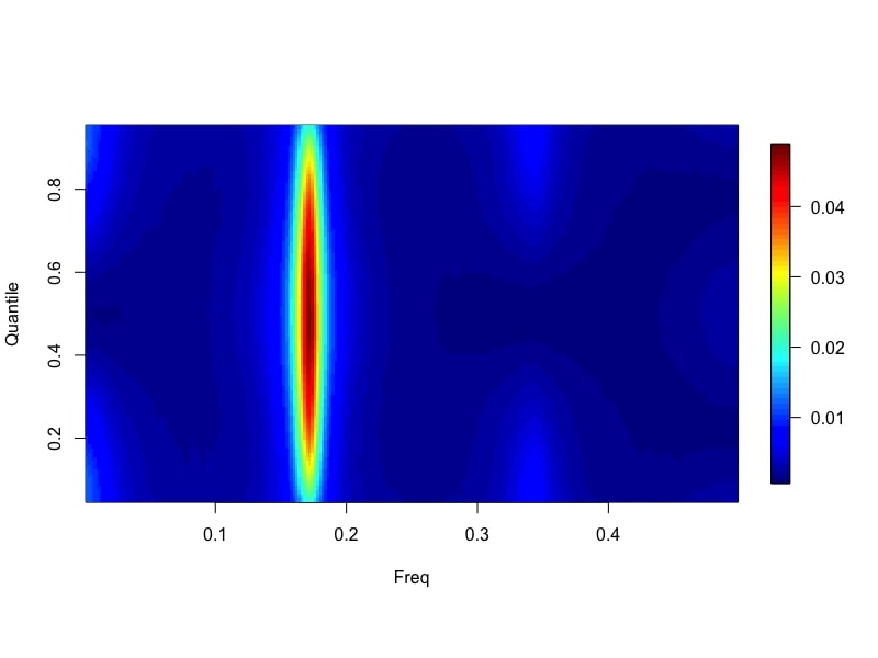
(a) Quantile spectrum of model 1

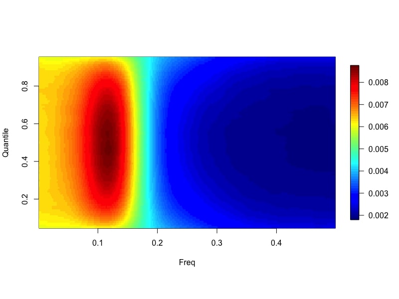
(b) Quantile spectrum of model 2

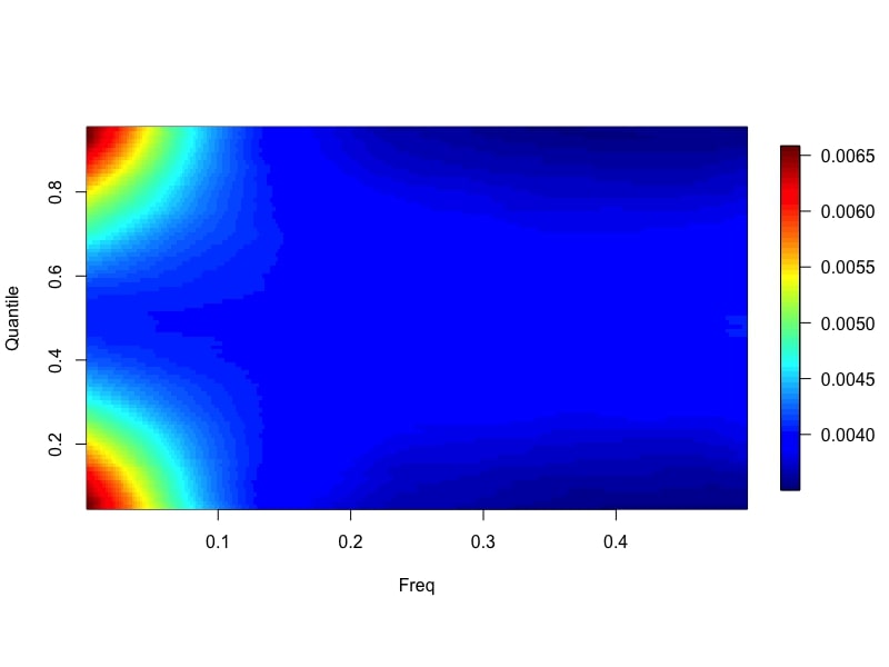
(c) Quantile spectrum of model 3

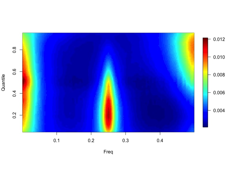
(d) Quantile spectrum of model 4

Figure 1: The true quantile spectra of the four models (n=500). (a) AR(2) model, (b)ARMA(2,2) model, (c) GARCH(1,1) model and (d) mixture model.

3.2 Comparisons

We compare our proposed algorithm to three commonly used smoothing methods: spline smoothing, Gamma-GCV smoothing (Ombao et al.,, 2001), and 2D Gaussian kernel smoothing. For the spline and Gamma-GCV smoothing, at each quantile level $\tau_{i}$, $i=1,...,m$, we apply the smoothing methods to the raw quantile periodograms $Q_{n,\tau_{i}}(\omega)$, and then smooth across the quantile levels for each frequency using splines. We select the tuning parameter for spline smoothing by ordinary leave-one-out cross-validation (function smooth.spline in R). We also apply the 2D Gaussian kernel smoothing to the raw quantile periodograms. These three methods, as well as the proposed method, all consider the smoothness of both the frequencies (horizontal) and the quantile levels (vertical).

We use the divergence between the results of each of the estimators and the ground truth to measure the performance. For GARCH models, we only consider the first 1/5 frequencies. For each simulation run of each estimator, we compute the divergence between the estimator and the ground truth at each quantile level $\tau_{i}$, $i=1,...,m$, and then average the $m$ distances across the quantile levels. Finally, we use the averaged divergences from the N=200 simulation runs of each estimator to assess performance.

We consider two spectral divergence measures:

• Kullback-Leibler (KL) divergence (Kullback and Leibler,, 1951):

  $$D_{KL}\{\tilde{f}_{1,\tau_{i}}(\omega),\tilde{f}_{2,\tau_{i}}(\omega)\}=\sum_{l}\tilde{f}_{1}(\omega_{l}){\sf ln}\frac{\tilde{f}_{2}(\omega_{l})}{\tilde{f}_{1}(\omega_{l})}.$$

• Root mean squared error (RMSE):

  $$D_{RMSE}\{\tilde{f}_{1,\tau_{i}}(\omega),\tilde{f}_{2,\tau_{i}}(\omega)\}=\sqrt{\frac{1}{n}\sum_{l=0}^{n-1}\left[\tilde{f}_{1,\tau_{i}}(\omega_{l})-\tilde{f}_{2,\tau_{i}}(\omega_{l})\right]^{2}}.$$

3.3 Simulation Results

The divergence error from each scenario averaged over N=200 simulations are shown in Tables 1 and 2. The minimum value in each of the four methods in each row is shown in bold. We also include the standard error in the tables.

Model	n	Parametric	Spline	Gamma-GCV	2D kernel
AR(2)	500	0.366(0.151)	0.667(0.338)	0.632(0.165)	1.606(0.303)
AR(2)	1000	0.233(0.085)	0.429(0.218)	0.357(0.088)	1.643(0.226)
AR(2)	2000	0.137(0.045)	0.240(0.088)	0.195(0.051)	1.678(0.160)
ARMA(2,2)	500	0.124(0.039)	0.156(0.052)	0.172(0.041)	1.631(0.142)
ARMA(2,2)	1000	0.074(0.024)	0.089(0.028)	0.164(0.030)	1.650(0.089)
ARMA(2,2)	2000	0.042(0.010)	0.051(0.015)	0.159(0.021)	1.686(0.070)
GARCH(1,1)	500	0.030(0.025)	0.042(0.036)	0.111(0.050)	1.551(0.185)
GARCH(1,1)	1000	0.020(0.012)	0.024(0.018)	0.131(0.046)	1.633(0.156)
GARCH(1,1)	2000	0.015(0.008)	0.016(0.010)	0.142(0.031)	1.679(0.106)
Mixture	500	0.227(0.062)	0.257(0.088)	0.234(0.050)	1.647(0.124)
Mixture	1000	0.139(0.033)	0.154(0.040)	0.185(0.032)	1.650(0.092)
Mixture	2000	0.082(0.019)	0.092(0.028)	0.169(0.023)	1.593(0.060)

Table 1: The averaged KL divergences to the ground truth from 200 simulation runs and the standard errors ($\times 10^{-1}$).

Model	n	Parametric	Spline	Gamma-GCV	2D kernel
AR(2)	500	1.945(0.461)	2.489(0.796)	2.699(0.401)	4.124(0.934)
AR(2)	1000	0.806(0.170)	1.046(0.340)	1.054(0.143)	2.181(0.368)
AR(2)	2000	0.313(0.067)	0.399(0.099)	0.352(0.071)	1.132(0.153)
ARMA(2,2)	500	0.660(0.124)	0.741(0.144)	0.791(0.115)	2.751(0.183)
ARMA(2,2)	1000	0.255(0.046)	0.281(0.051)	0.399(0.046)	1.386(0.061)
ARMA(2,2)	2000	0.099(0.013)	0.108(0.017)	0.202(0.017)	0.703(0.024)
GARCH(1,1)	500	0.548(0.134)	0.546(0.141)	0.791(0.150)	2.654(0.247)
GARCH(1,1)	1000	0.215(0.051)	0.213(0.052)	0.402(0.063)	1.364(0.107)
GARCH(1,1)	2000	0.082(0.018)	0.082(0.019)	0.201(0.022)	0.697(0.036)
Mixture	500	0.956(0.141)	1.004(0.171)	0.958(0.118)	2.622(0.178)
Mixture	1000	0.378(0.050)	0.393(0.056)	0.426(0.048)	1.355(0.069)
Mixture	2000	0.145(0.019)	0.153(0.024)	0.205(0.019)	0.687(0.022)

Table 2: The averaged RMSEs to the ground truth from 200 simulation runs and the standard errors ($\times 10^{-3}$).

From Tables 1 and 2, we see that the proposed method outperforms the three conventional methods. The proposed method results the smallest divergence to the ground truth under most conditions. There are two exceptions: GARCH model ($n=500,1000$) using RMSE, while the differences are less than $10^{-5}$. Additionally, the divergences and the standard errors show a decreasing trend as $n$ increases.

4 Earthquake Data Application

In this section, we apply our method to an earthquake classification problem. We first describe the data in Section 4.1 and then present the quantile periodogram analysis in Section 4.2. The classification of the smoothed quantile periodogram using the CNN is illustrated in Section 4.3.

4.1 Data Description

The earthquake data in this section is waveform data collected during February 2014 in Oklahoma (USA). The continuous waveform data and earthquake catalog are publicly available at
https://www.iris.edu/hq/ and http://www.ou.edu/ogs.html. Details about the catalog data are provided in Benz et al., (2015), where the magnitudes and times of the earthquakes are labeled. The waveform data we use is from 2014-02-15 00:00:00.005 to 2014-02-28 23:59:58.995, and has a sampling rate of 100 Hz.

4.2 Quantile Periodogram Analysis

From the original dataset, there are ten earthquakes with magnitudes greater than 3. Information about the ten earthquakes is shown in Table 3. We extract eight epochs, each comprising one hour of data surrounding one such earthquake event if it is separated from the others by more than one hour or two such earthquake events if they are separated by less than one hour. The total sample size is 2,888,000 (360,000$\times$8). For each epoch, we use a moving window with a width of 20 seconds and move forward at 10 seconds per step, which generates 359 time series of waveform data for each epoch. In each window, the time series is subtracted by a spline fit to eliminate the low-frequency components that do not differ between the earthquake windows and no-earthquake windows. For each time series, we estimate the quantile spectrum using the proposed method and use the first half of the frequencies ($l=1,...,500$) at quantiles {0.05,0.06,…,0.95}. The advantage of using a moving window with an overlap is that, for most cases, the earthquakes appear in at least two frames, which makes the visualization easier. The animations that show the evolution of the smoothed periodogram over time for each epoch can be viewed in the supplementary files.

Date	Time	Magnitude
02-15-2014	00:19:12	3.51
02-16-2014	01:51:47	3.47
02-17-2014	04:54:59	3.50
02-17-2014	05:02:11	3.07
02-17-2014	08:24:21	3.05
02-17-2014	14:19:13	3.36
02-18-2014	11:53:50	3.15
02-18-2014	12:16:43	3.12
02-19-2014	16:44:56	3.25
02-21-2014	21:38:49	3.06

Table 3: Information about the ten earthquakes from February 2014.

Four representative windows from the animations are shown in Figure 2, where the window in Figure 2(a) contains a very large earthquake with a magnitude of 3.47; the window in Figure 2(b) contains a somehow large earthquake with a magnitude of 1.32; (3) the window in Figure 2(c) contains a tiny earthquake with a magnitude $<$ 0.1; and the window in Figure 2(d) does not contain an earthquake. By comparing these results, we have the following findings:

• The smoothed quantile periodogram in the presence of a large earthquake has a large peak at the low-frequency band in the high and low quantiles (see Figure 2 (a) and (b)).

• The smoothed quantile periodogram without an earthquake has peaks at a higher frequency band (see Figure 2(d)).

• The smoothed quantile periodogram in the presence of a very small earthquake has peaks at both low frequency band (in low and high quantiles) and high frequency band (in middle quantiles). The magnitude is too small to make the peak at low frequency band overwhelm the peaks at high frequency band (see Figure 2(c)).

  

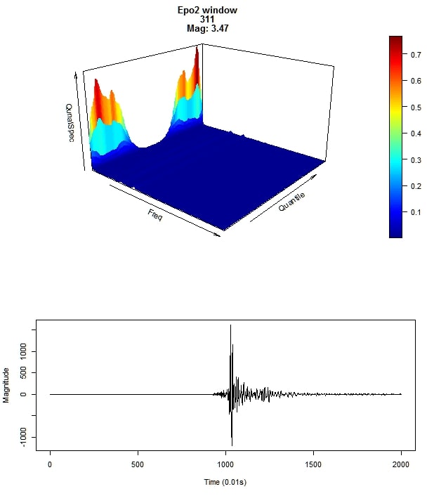
  (a) Earthquake window (mag: 3.47)

  

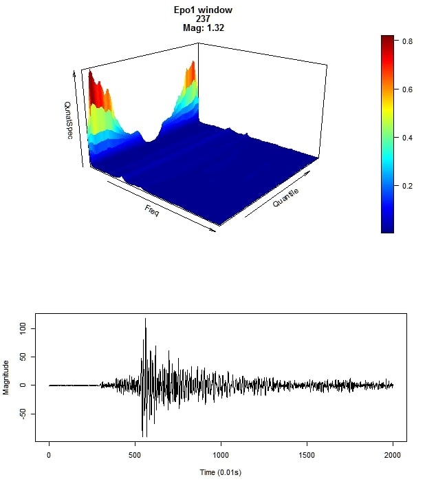
  (b) Earthquake window (mag: 1.32 )

  

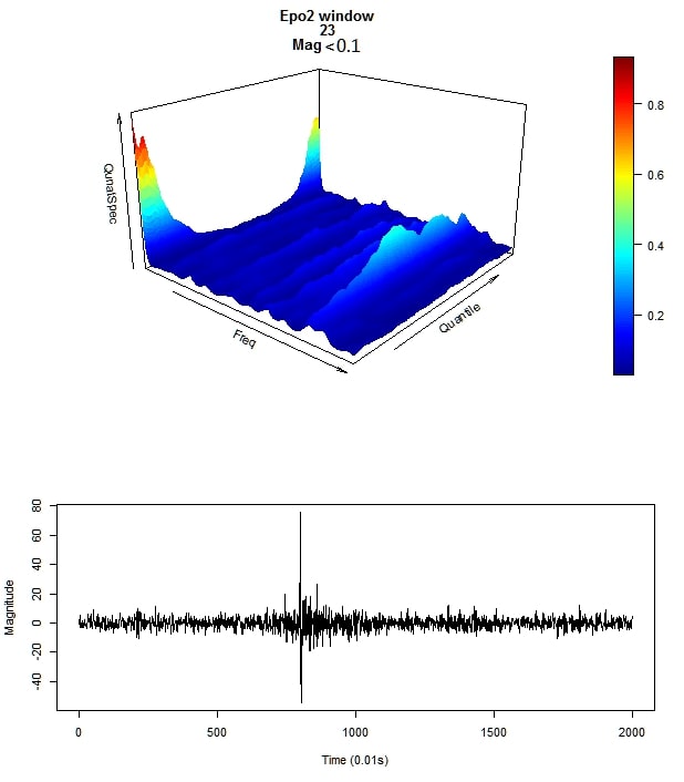
  (c) Earthquake window (mag$<$0.1)

  

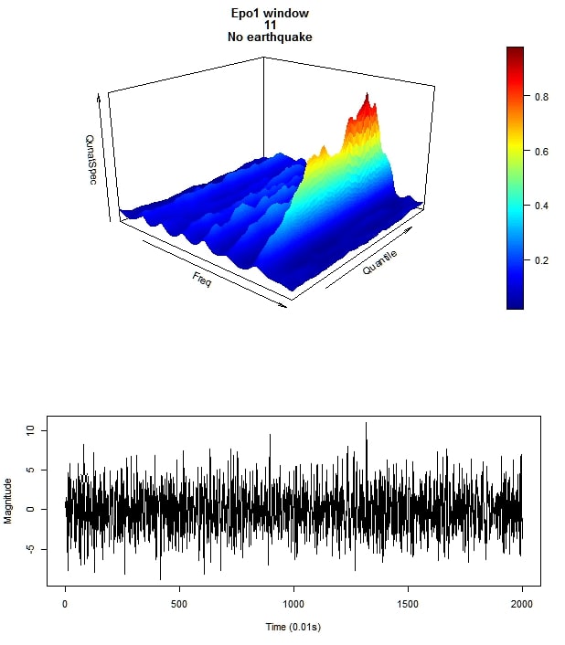
  (d) No earthquake window

  Figure 2: (a), (b), and (c) Windows with earthquakes. (d) The window without earthquakes. The top image in each window (a-d) shows a 3D plot of the smoothed quantile periodogram.

4.3 Classifications Using CNN

In this section, we use the smoothed quantile periodogram as a feature by which we classify the segments into those that contain earthquakes and those that do not. We treat the quantile spectrum as a 2D image and apply the CNN to build the classifier. We extract 2000 nonoverlapping segments of data, each being a time series of length 2000 (equivalent to 20 seconds). Among the 2000 segments, 1000 of them contain an earthquake with a magnitude higher than 0.25 and the remaining 1000 segments contain no earthquakes. In each segment, the time series is subtracted by a spline fit to eliminate the low-frequency components that do not differ between the earthquake segments and no-earthquake segments. The 2000 smoothed quantile periodogram (we use $l=1,...,500$) and their labels are the input data for the CNN. Since we use the normalized quantile periodograms, the amplitude is not considered; we focus on the serial dependence, which makes the classifications more challenging. We randomly split the segments into training and testing sets with respective sizes of 1600 and 400. We build the CNN with two convolution layers, each one connected to a maxpooling layer, where the second maxpooling layer connects to fully connected layers (FC). The CNN structure is shown in Figure 3(a).

To show the advantages of quantile periodograms, we also estimate the ordinary spectra using AR models, with the orders selected by AIC. We apply a CNN with the same structure with different dimensions of the input ($500\times 1$ instead of $500\times m$) and the kernel (5$\times$1 instead of 5$\times$5). We use ten random seeds to initialize the CNN training process and pick the one that yields the best performance. The training and testing accuracy curves are shown in Figure 3(b), and the confusion matrices are shown in Tables 4 and 5. The metrics we use are true positive (TP), which indicates that the segment has an earthquake and is classified as an earthquake; true negative (TN), which indicates that the segment has no earthquake and is classified as no earthquake; false positive (FP), which indicates that the segment has no earthquake but is classified as an earthquake; false negative (FN), which indicates that the segment has an earthquake but is classified as no earthquake. From these results, we see that

• The classification based on quantile periodograms has a higher accuracy rate. Specifically, for quantile periodograms, the accuracy is 100.00% (training) and 99.25% (testing); for ordinary periodograms, the accuracy is 99.56% (training) and 98.00% (testing).

• No misclassification in training set and higher precision ($\frac{TP}{TP+FP}$) and recall ($\frac{TP}{TP+FN}$) using quantile periodograms.

• One misclassification case using quantile periodograms is shown in Figure 3(c). Since the magnitude is small, the power at low frequencies is not as large as the power at high frequencies, which cause the misclassification.

	Positive	Negative
True	800	800
False	0	0

(a) Training set

	Positive	Negative
True	198	199
False	1	2

(b) Testing set

	Positive	Negative
True	998	999
False	1	2

(c) Total

Table 4: The confusion matrices of the classification using quantile periodograms.

	Positive	Negative
True	795	798
False	2	5

(a) Training set

	Positive	Negative
True	193	199
False	1	7

(b) Testing set

	Positive	Negative
True	988	997
False	3	12

(c) Total

Table 5: The confusion matrices of the classification using ordinary periodograms.

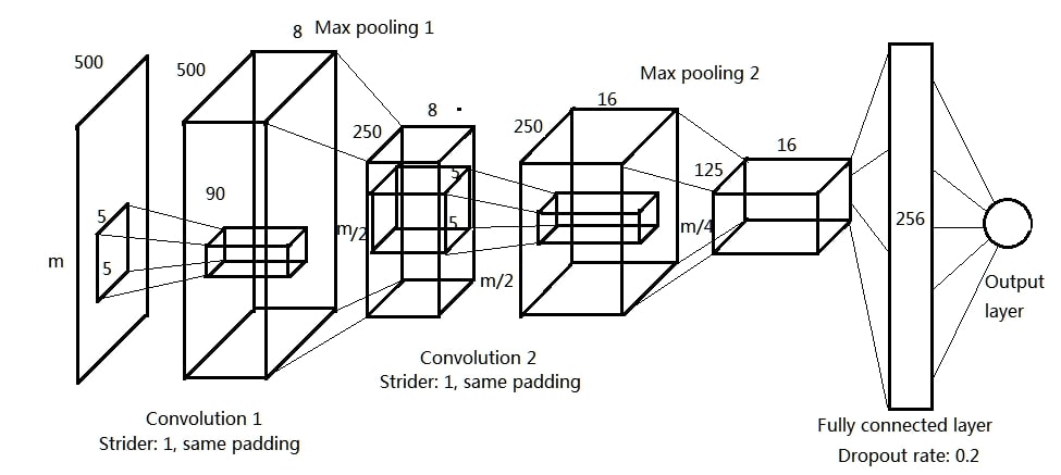
(a) CNN structure

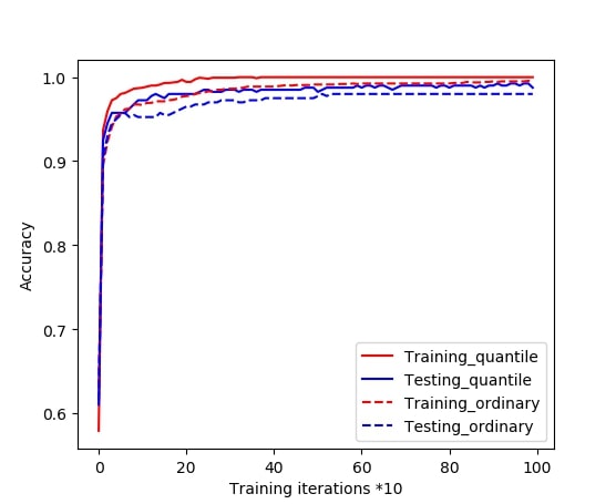
(b) Accuracy curves

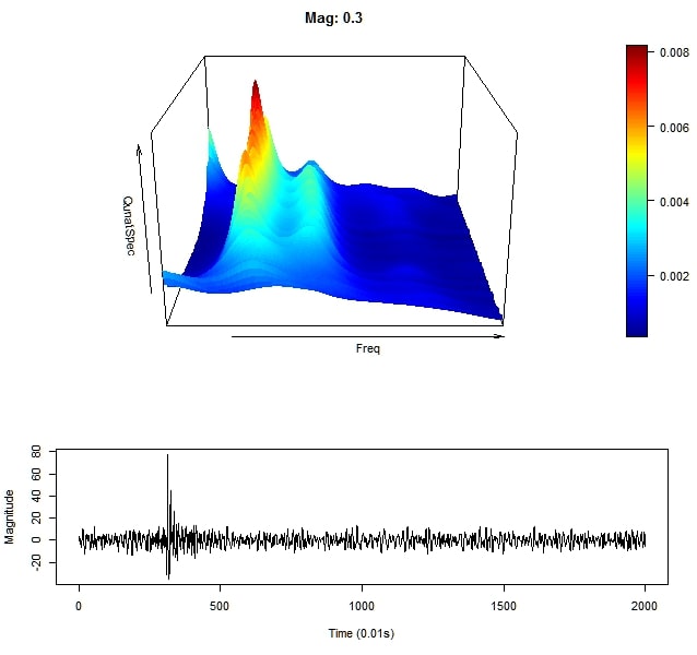
(c) Misclassification case

Figure 3: (a) The CNN structure, (b) the training and testing accuracy of quantile periodograms and ordinary periodograms, and (c) the misclassification case when using quantile periodograms.

5 Conclusion

In this paper, we proposed a new semi-parametric estimation method for the quantile spectrum that uses a parametric form of the AR approximation coupled with nonparametric smoothing. Based on the AR approximation theorem and the maximum entropy principle, we approximate the quantile spectrum by the ordinary AR spectral density at each quantile level. At each quantile level, we define the QACF as the inverse Fourier transform of the raw quantile periodogram. By solving the Yule-Walker equations using the Levinson-Durbin algorithm, we obtain the QPACF and the residual variance from the QACF. The AR order at each quantile is selected by minimizing the AIC, thus balancing the goodness of fit and the model complexity. Then, we smooth the AR orders and the residual variances across the quantile level to reduce variability. Finally, the quantile AR coefficients, obtained from the smoothed QPACF across quantile levels, are used to construct the quantile spectrum. In such a way, the quantile periodogram is smoothed across both the quantile levels and the frequencies. Equipped with the smoothed quantile periodogram, we are able to use the 2D image classification techniques to classify time series. In particular, we apply the CNN, which is a powerful tool for image classification, with the quantile periodogram as input.

The 2D property of the quantile periodogram means that it provides more information than the ordinary periodogram, and that we can take advantage of advanced techniques for images to analyze the time series data. The quantile regression technique also endows the quantile periodogram with sufficient robustness to handle noisy data with outliers. However, the quantile periodogram incurs a higher computational cost because its dimension is multiplied by the number of quantiles. If the scale is not of primary interest, one can use conventional FFT method applied to the clipped data (see Kley, (2016) and R package quantspec), which is less efficient statistically but easier to compute, to obtain the level-crossing periodogram instead of using quantile regression to reduce the computational cost. Li, (2008) and Li, (2010) compared the statistical efficiency of quantile-regression based method and the hard clipping method for hidden periodicity detection and estimation. In the classification procedure using CNN (Section 4.3), the training time was 1.96 seconds per iteration when using quantile periodograms, but only 0.02 seconds per iteration when using ordinary periodograms. One solution to reduce the computational cost is to use fewer quantiles. In this paper, we use a large number of quantiles to make the estimator more like an image. In other applications, we may only look at a few quantiles with sufficient discriminative power, e.g., high or low quantiles. We also used multicore parallelization to speed up computing the raw quantile periodograms.

6 Acknowledgement

This research was supported by funding from King Abdullah University of Science and Technology (KAUST). We would like to thank the editor, associate editor, and reviewers for their valuable comments.

References

- Akaike, (1974) Akaike, H. (1974). A new look at the statistical model identification. IEEE Transactions on, Automatic Control, 19(6):716–723.
- Barndorff-Nielsen and Schou, (1973) Barndorff-Nielsen, O. and Schou, G. (1973). On the parametrization of autoregressive models by partial autocorrelations. Journal of multivariate Analysis, 3(4):408–419.
- Baruník and Kley, (2019) Baruník, J. and Kley, T. (2019). Quantile coherency: A general measure for dependence between cyclical economic variables. The Econometrics Journal, 22(2):131–152.
- Benz et al., (2015) Benz, H. M., McMahon, N. D., Aster, R. C., McNamara, D. E., and Harris, D. B. (2015). Hundreds of earthquakes per day: The 2014 guthrie, oklahoma, earthquake sequence. Seismological Research Letters, 86(5):1318–1325.
- Birr et al., (2019) Birr, S., Kley, T., and Volgushev, S. (2019). Model assessment for time series dynamics using copula spectral densities: a graphical tool. Journal of Multivariate Analysis, 172:122–146.
- Birr et al., (2017) Birr, S., Volgushev, S., Kley, T., Dette, H., and Hallin, M. (2017). Quantile spectral analysis for locally stationary time series. Journal of the Royal Statistical Society: Series B (Statistical Methodology), 79(5):1619–1643.
- Brockwell and Davis, (1984) Brockwell, P. J. and Davis, R. A. (1984). Time Series: Theory and Methods. Springer.
- Brockwell and Davis, (2006) Brockwell, P. J. and Davis, R. A. (2006). Time Series: Theory and Methods. Springer.
- Broersen and Wensink, (1998) Broersen, P. M. and Wensink, H. E. (1998). Autoregressive model order selection by a finite sample estimator for the kullback-leibler discrepancy. IEEE Transactions on Signal Processing, 46(7):2058–2061.
- Capon, (1983) Capon, J. (1983). Maximum-likelihood spectral estimation. Nonlinear Methods of Spectral Analysis, 34(1):155–179.
- Chan and Langford, (1982) Chan, Y. and Langford, R. (1982). Spectral estimation via the high-order yule-walker equations. IEEE Transactions on Acoustics, Speech, and Signal Processing, 30(5):689–698.
- Chow and Grenander, (1985) Chow, Y.-S. and Grenander, U. (1985). A sieve method for the spectral density. The Annals of Statistics, 13(3):998–1010.
- Dette et al., (2015) Dette, H., Hallin, M., Kley, T., Volgushev, S., et al. (2015). Of copulas, quantiles, ranks and spectra: An -approach to spectral analysis. Bernoulli, 21(2):781–831.
- Engle, (1982) Engle, R. F. (1982). Autoregressive conditional heteroscedasticity with estimates of the variance of united kingdom inflation. Econometrica: Journal of the Econometric Society, 50(4):987–1007.
- Friedlander and Porat, (1984) Friedlander, B. and Porat, B. (1984). The modified yule-walker method of arma spectral estimation. IEEE Transactions on Aerospace and Electronic Systems, (2):158–173.
- Friedman, (1984) Friedman, J. H. (1984). A variable span smoother. Technical report, Stanford Univ CA lab for computational statistics.
- Hagemann, (2013) Hagemann, A. (2013). Robust spectral analysis. arXiv preprint arXiv:1111.1965.
- Hurvich and Tsai, (1989) Hurvich, C. M. and Tsai, C.-L. (1989). Regression and time series model selection in small samples. Biometrika, 76(2):297–307.
- Kley, (2016) Kley, T. (2016). Quantile-based spectral analysis in an object-oriented framework and a reference implementation in r: The quantspec package. Journal of Statistical Software, Articles, 70(3):1–27.
- Koenker, (2005) Koenker, R. (2005). Quantile regression. Cambridge University Press.
- Krizhevsky et al., (2012) Krizhevsky, A., Sutskever, I., and Hinton, G. E. (2012). Imagenet classification with deep convolutional neural networks. In Advances in neural information processing systems, pp. 1097-1105.
- Kullback and Leibler, (1951) Kullback, S. and Leibler, R. A. (1951). On information and sufficiency. The annals of mathematical statistics, 22(1):79–86.
- Lee, (1997) Lee, T. C. (1997). A simple span selector for periodogram smoothing. Biometrika, 84(4):965–969.
- Li, (2008) Li, T.-H. (2008). Laplace periodogram for time series analysis. Journal of the American Statistical Association, 103(482):757–768.
- Li, (2010) Li, T.-H. (2010). Robust coherence analysis in the frequency domain. In 2010 18th European Signal Processing Conference, pages 368–371. IEEE.
- (26) Li, T.-H. (2012a). Detection and estimation of hidden periodicity in asymmetric noise by using quantile periodogram. In Proceedings of the IEEE International Conference on Acoustics, Speech and Signal Processing (ICASSP),vol 2, pp. 3969-3972.
- (27) Li, T.-H. (2012b). Quantile periodograms. Journal of the American Statistical Association, 107(498):765–776.
- Li, (2013) Li, T.-H. (2013). Time series with mixed spectra. Chapman and Hall/CRC.
- Li, (2014) Li, T.-H. (2014). Quantile periodogram and time-dependent variance. Journal of Time Series Analysis, 35(4):322–340.
- Lim and Oh, (2016) Lim, Y. and Oh, H.-S. (2016). Composite quantile periodogram for spectral analysis. Journal of Time Series Analysis, 37(2):195–221.
- Maadooliat et al., (2018) Maadooliat, M., Sun, Y., and Chen, T. (2018). Nonparametric collective spectral density estimation with an application to clustering the brain signals. To appear in Statistics in Medicine.
- Ombao et al., (2001) Ombao, H. C., Raz, J. A., Strawderman, R. L., and Von Sachs, R. (2001). A simple generalised crossvalidation method of span selection for periodogram smoothing. Biometrika, 88(4):1186–1192.
- Orhan et al., (2011) Orhan, U., Hekim, M., and Ozer, M. (2011). Eeg signals classification using the k-means clustering and a multilayer perceptron neural network model. Expert Systems with Applications, 38(10):13475–13481.
- Parzen, (1957) Parzen, E. (1957). On consistent estimates of the spectrum of a stationary time series. The Annals of Mathematical Statistics, pages 329–348.
- Pawitan and O’Sullivan, (1994) Pawitan, Y. and O’Sullivan, F. (1994). Nonparametric spectral density estimation using penalized whittle likelihood. Journal of the American Statistical Association, 89(426):600–610.
- Schwarz et al., (1978) Schwarz, G. et al. (1978). Estimating the dimension of a model. The annals of statistics, 6(2):461–464.
- Shumway and Stoffer, (2011) Shumway, R. H. and Stoffer, D. S. (2011). Spectral analysis and filtering. In Time Series Analysis and Its Applications, pp. 173-265. Springer.
- Shumway and Stoffer, (2016) Shumway, R. H. and Stoffer, D. S. (2016). Time series analysis and its applications: with R examples. Springer Science & Business Media.
- Wahba, (1980) Wahba, G. (1980). Automatic smoothing of the log periodogram. Journal of the American Statistical Association, 75(369):122–132.
- Whittle, (1953) Whittle, P. (1953). Estimation and information in stationary time series. Arkiv för matematik, 2(5):423–434.
- Whittle, (1954) Whittle, P. (1954). Some recent contributions to the theory of stationary processes. A study in the analysis of stationary time series, 2:196–228.
- Zhang, (2019) Zhang, S. (2019). Bayesian copula spectral analysis for stationary time series. Computational Statistics & Data Analysis, 133:166–179.