Quasi-one-dimensional approximation for Bose-Einstein condensates transversely trapped by a funnel potential

Abstract

Starting from the standard three-dimensional (3D) Gross-Pitaevskii equation (GPE) and using a variational approximation, we derive an effective one-dimensional nonpolynomial Schrödinger equation (1D-NPSE) governing the axial dynamics of atomic Bose-Einstein condensates (BECs) under the action of a singular but physically relevant funnel-shaped transverse trap, i.e., an attractive 2D potential $\sim-1/r$ (where $r$ is the radial coordinate in the transverse plane), in combination with the repulsive self-interaction. Wave functions of the trapped BEC are regular, in spite of the potential’s singularity. The model applies to a condensate of particles (small molecules) carrying a permanent electric dipole moment in the field of a uniformly charged axial thread, as well as to a quantum gas of magnetic atoms pulled by an axial electric current. By means of numerical simulations, we verify that the effective 1D-NPSE provides accurate static and dynamical results, in comparison to the full 3D GPE, for both repulsive and attractive signs of the intrinsic nonlinearity.

I Introduction

The observation of the Bose-Einstein condensation (BEC) in alkali-metal atomic gas at ultralow temperatures was reported 70 years after it was predicted Anderson et al. (1995); Davis et al. (1995); Bradley et al. (1997). Currently, BECs are produced and manipulated by various research groups, for various kinds of atomic species Griesmaier et al. (2005); Fried et al. (1998); Aikawa et al. (2012), and are also observed in molecular gases Jochim et al. (2003); Zwierlein et al. (2003). These setting give rise to countless effects, such as the formation of matter-wave dark Burger et al. (1999); Denschlag et al. (2000) and bright Khaykovich et al. (2002) solitons, propagation of matter-wave soliton trains Strecker et al. (2002), creation of vortex states Matthews et al. (1999); Madison et al. (2000), prediction of stable vortex solitons in various forms Malomed (2019), observation of Feshbach resonances Inouye et al. (1998), etc. A recent addition to this list is the prediction Petrov (2015); Petrov and Astrakharchik (2016) and experimental creation Cabrera et al. (2018); Cheiney et al. (2018); Semeghini et al. (2018); Ferioli et al. (2019); D’Errico et al. (2019) of multidimensional “quantum droplets”, in which the matter-wave collapse is arrested by the Lee-Huang-Yang (LHY) effect, produced by fluctuational corrections to the mean-field dynamics.

The study of static and dynamical properties of dilute BECs at zero temperature is accurately modeled by the time-dependent three-dimensional (3D) Gross-Pitaevskii equation (GPE) Pitaevskii and Stringari (2003); Pethick and Smith (2008) (if necessary, complemented by the above-mentioned LHY terms Petrov (2015); Petrov and Astrakharchik (2016)). A relevant problem is to reduce the full three-dimensional GPE to lower-dimensional equations, when the reduction is imposed by an external potential which tightly confines BEC in one or two transverse directions. Several approximations for the dimensional reductions 3D $\rightarrow$ 1D and 3D $\rightarrow$ 2D were elaborated, for both self-repulsive and attractive signs of the nonlinearity in GPE Muryshev et al. (2002); Salasnich et al. (2002a, b); Massignan and Modugno (2003); Kamchatnov and Shchesnovich (2004); Carr and Brand (2004); Zhang and You (2005); Salasnich and Malomed (2006); Matuszewski Michałand Królikowski et al. (2006); Wei et al. (2007); Salasnich et al. (2007a, b); Mateo and Delgado (2007); Maluckov et al. (2008); Salasnich et al. (2008); Salasnich (2009); Li et al. (2009); Buitrago and Adhikari (2009); Adhikari and Salasnich (2009); Salasnich and Malomed (2009); Muñoz Mateo and Delgado (2009); Young-S. et al. (2010); Cardoso et al. (2011); Mateo et al. (2011); Edwards et al. (2012); Díaz et al. (2012); Salasnich and Malomed (2013); Salasnich et al. (2014); Chiquillo (2015); dos Santos and Cardoso (2019). In particular, the use of the variational approximation (VA) for the transverse profile of the wave function, presented in Refs. Salasnich et al. (2002a, b), helps to derive an effective 1D nonpolynomial Schrödinger equation (1D-NPSE), which accurately models the axial dynamics of the cigar-shaped BECs Cuevas et al. (2013). This method can also be applied for the derivation of effective 2D-NPSEs, when BEC is strongly confined in the axial direction Salasnich et al. (2002a); Salasnich and Malomed (2009). This method can be used to analyze the evolution of elongated BECs with Massignan and Modugno (2003) or without Kamchatnov and Shchesnovich (2004) the assumption that the wave function slowly varies along the axial direction, dynamics of spin-1 condensates Zhang and You (2005), and binary self-attractive BECs Salasnich and Malomed (2006), as well as the behavior of BEC in a nearly-1D cigar-shaped trap with the transverse confining frequency periodically modulated along the axial direction De Nicola et al. (2006); Salasnich et al. (2007a, b); Maluckov et al. (2008), effects of embedded axial vorticity in the elongated BECs Salasnich et al. (2008), matter waves under anisotropic transverse confinement Salasnich (2009), BECs in funnel- Li et al. (2009) and tube-shaped dos Santos and Cardoso (2019) potentials, mean-field equations for cigar- and disc-shaped Bose-Fermi mixtures and fermion superfluids Buitrago and Adhikari (2009); Adhikari and Salasnich (2009); Díaz et al. (2012), solitons and solitary vortices in BECs Salasnich and Malomed (2009), BECs in mixed dimensions Young-S. et al. (2010), dilute bosonic gases with intrinsic two- and three-body interactions Cardoso et al. (2011), BECs confined in ring-shaped potentials Edwards et al. (2012), BECs with spin-orbit and Rabi couplings Salasnich and Malomed (2013); Salasnich et al. (2014); Chiquillo (2015); Li et al. (2017, 2018), etc.

In this work, we consider BEC confined by a funnel-shaped potential acting in the transverse plane $\left(x,y\right)$, i.e., the 2D attractive potential

$$V_{\mathrm{transverse}}(r)=-\frac{\varepsilon^{3}}{2r},$$ (1)

with $\varepsilon>0$ and transverse radial coordinate $r\equiv\sqrt{x^{2}+y^{2}}$. As suggested by Ref. Sakaguchi and Malomed (2011), this potential may be applied by an axially oriented wire, uniformly charged with density $\sigma$, to small molecules carrying a permanent dipole moment $\mathbf{d}$, which is oriented along the local electric field, with strength of the radial electric field $\mathbf{E}=2\sigma\boldsymbol{r}/r^{2}$ (the interaction of a neutral polarizable atom with a uniformly charged wire was considered in Ref. Denschlag and Schmiedmayer (1997)). Then, indeed, the potential pulling the dipoles to the axis is $V_{\mathrm{transverse}}(r)=-\mathbf{d}\cdot\mathbf{E}\equiv-2\sigma d/r$, which is tantamount to potential (1). A still more realistic possibility is provided by a quantum gas of atoms carrying permanent magnetic moments (such as chromium, dysprosium, or erbium Griesmaier et al. (2005); Ferrier-Barbut et al. (2016); Schmitt et al. (2016); Chomaz et al. (2016)), pulled in the axial direction by an electric-current jet (which may be an electronic beam) Sakaguchi and Malomed (2011).

With the help of VA, we derive an effective 1D equation describing the axial dynamics in this setting. A similar configuration was considered in Ref. Li et al. (2009). However, unlike that work, which used VA based on the Gaussian ansatz, we employ one with an exponential profile. This difference is more than a formal modification, as the exponential approximation agrees with the specific asymptotic form of the wave function at $r\rightarrow 0$, imposed by the singularity of the funnel trap (see Eq. ((5)) below), while the Gaussian ansatz contradicts it. As a result, full 3D numerical simulations demonstrate that we obtain a more accurate model equation for the BEC confined by the funnel-shaped potential (in fact, no solutions of the 1D equation, nor the asymptotic form of the 3D wave function, were considered in Ref. Li et al. (2009)). Limit cases, pertaining to weak- and strong-coupling regimes, are also considered, as well as results provided by the effective equation derived in Ref. Li et al. (2009), for the comparison’s sake. Further, we demonstrate that the effective NPSE obtained here also provides an accurate approximation for the transverse width of the confined BEC.

The rest of the paper is organized as follows. In the next section, starting from the 3D GPE and using the VA, we derive an effective NPSE governing the axial dynamics in the funnel-shaped configuration. Limit cases of the NPSE, and a similar effective 1D equation which was derived, in a more formal way, in Ref. Li et al. (2009) are addressed in the same section. Systematic numerical results, for both the static ground states (GSs) and dynamical regimes, are reported in Sec. III. The paper is concluded by Sec. IV.

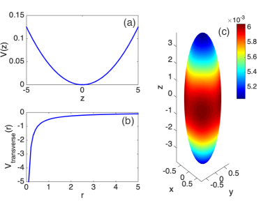
Figure 1: The confining potential, given by Eqs. (3) and (17), in the axial (a) and radial (b) directions. (c) A schematic shape of the density in the respective 3D ground state.

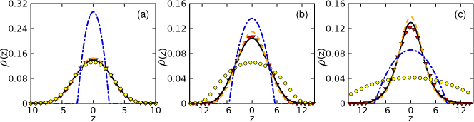
Figure 2: Normalized axial density profiles $\rho(z)$ for a repulsive BEC ($g>0$), under the combined action of the funnel trap (1) with $\varepsilon=1$ and axial potential (17) with $\lambda=0.1$, for (a) $g=1$, (b) $g=10$, and (c) $g=40$. The density profiles were numerically obtained as GS (ground-state) solutions of the full 3D GPE (4) (red triangles), 1D-NPSE (12) (the black solid line black), 1D YXWLH equation (14) (the orange dashed line), cubic 1D-NLSE (15) (yellow circles), and the TF state (16) (the blue dashed-dotted line).

II The derivation of the effective nonpolynomial Schrödinger equation

A monatomic BEC at zero temperature is modeled by the commonly known 3D GPE,

$$i\hbar\frac{\partial\psi}{\partial t}=-\frac{\hbar^{2}}{2m}\mathbf{\nabla}^{2}\psi+V(r,z)\psi+\mathcal{N}U|\psi|^{2}\psi,$$ (2)

where $\psi(\mathbf{r},t)$ is the mean-field wave function of the condensate, potential

$$V(r,z)\equiv-\frac{\varepsilon^{3}}{2r}+V(z)$$ (3)

includes the funnel trapping term (1) and a generic (nonsingular) axial one, $V(z)$, $U\equiv 4\pi\hbar^{2}a_{s}/m$ is the nonlinearity strength, with $a_{s}>0$ being the atomic s-wave scattering length of repulsive interatomic interactions, and $\mathcal{N}$ is the number of condensed atoms. By means of rescaling $t\rightarrow\omega_{r}t$, $(x,y,z)\rightarrow(x,y,z)/a_{r}$, $\psi\rightarrow\psi a_{r}^{3/2}$, with $a_{r}$ being a characteristic length scale in the transverse direction, Eq. (2) is cast in the normalized form,

$$i\frac{\partial\psi}{\partial t}=-\frac{1}{2}\mathbf{\nabla}^{2}\psi+V\left(r,z\right)\psi+2\pi g|\psi|^{2}\psi,$$ (4)

with $g\equiv 2\mathcal{N}a_{s}/a_{r}$.

As concerns the above-mentioned physical interpretation of the model in terms of the condensate of small molecules carrying the permanent electric moment, which are pulled to the uniformly charged axial wire, the respective GPE must take into account the long-range dipole-dipole interaction between the particles. As shown in Ref. Sakaguchi and Malomed (2011), this can be done by introducing a mean-field electrostatic field, which is induced by the effective charge density in the dipolar gas (as per the respective Poisson equation), $\mathbf{E}_{d}=-4\pi\left|\psi\left(x,y,z\right)\right|^{2}\mathbf{d}$. This, in turn, gives rise to effective renormalization of the scattering length, which is written in terms of the unscaled notation, $a_{s}\rightarrow a_{s}+md^{2}/\hbar^{2}$. Similarly, the mean-field approximation makes it possible to take into account dipole-dipole interactions between magnetic atoms.

A schematic representation of the trapping potential (3), and expected distribution of the BEC density in the corresponding GS is displayed in Fig. 1. Here, the axial term of the potential, $V(z)$, is assumed to take the harmonic-oscillator (HO) form, see Eq. (17) below.

In spite of the presence of the singular potential (1), Eq. (4) gives rise to a GS wave function with chemical potential $\mu$ and a regular expansion at $r\rightarrow 0$:

$$\psi\left(r,z.t\right) = e^{-i\mu t}\left[\left(1-\varepsilon^{3}r\right)\psi_{0}(z)+\frac{1}{2}\psi_{2}(z)r^{2}+...\right],$$ (5)

$$\psi_{2}(z) = \left(\frac{1}{2}\varepsilon^{6}-\mu+V(z)\right)\psi_{0}(z)+2\pi g\psi_{0}^{3}(z)-\frac{1}{2}\psi_{0}^{\prime\prime}(z)$$

[function $\psi_{0}(z)$ can be uniquely determined only from the global solution of Eq. (4), rather than solely from the expansion at small $r$]. An essential difference of Eq. (5) from a similar expansion constructed with a nonsingular potential is that, in the latter case, the expansion does not contain a term $\sim r$. On the other hand, it is relevant to stress that the GS does not exist in the presence of a more singular radial potential, viz., $V_{\mathrm{transverse}}(r)=-Cr^{-2},$ with $C>0$. In that case, one can formally find a wave function with a singularity at $r\rightarrow 0$, $\psi\sim r^{-1}$; however, this solution is unphysical, as its norm diverges Sakaguchi and Malomed (2011).

The Lagrangian density, corresponding to Eq. (4) with confining potential (3), is

$$\mathcal{L} = \frac{i}{2}\left(\psi^{\ast}\frac{\partial\psi}{\partial t}-\psi\frac{\partial\psi^{\ast}}{\partial t}\right)-\frac{1}{2}|\nabla\psi|^{2}$$ (6)

$$-\left(V(z)-\frac{\varepsilon^{3}}{2r}\right)|\psi|^{2}-\pi g|\psi|^{4}.$$

Our goal is to reduce the 3D model to an appropriate 1D approximation. To this end, we consider the following factorized ansatz:

$$\psi(r,z,t)=\exp\left(-\frac{r}{2\eta^{2}}\right)\frac{f(z,t)}{\sqrt{2\pi}\eta^{2}},$$ (7)

were $f(z,t)$ is an axial wave function, and $\eta=\eta(z,t)$ is the transverse width, with the normalization condition

$$\int_{-\infty}^{+\infty}|f\left(z\right)|{{}^{2}dz}=1,$$ (8)

which provides unitary normalization of the full 3D wave function (6). Note that the expansion of ansatz (7) at $r\rightarrow 0$ agrees with the asymptotic form given by Eq. (5).

The effective 1D-NPSE is produced by inserting ansatz (7) into Lagrangian density (6) and performing integration in the transverse plane, it being relevant to stress that the 2D integral with singular term $\sim 1/r$ in Eq. (6) converges. This procedure leads us to the following effective 1D Lagrangian,

$$L_{\mathrm{1D}} = \int_{-\infty}^{+\infty}\left[\frac{i}{2}\left(f^{\ast}\frac{\partial f}{\partial t}+\mathrm{c.c.}\right)-\frac{1}{2}\left|\frac{\partial f}{\partial z}\right|^{2}\right.$$ (9)

$$- \left.\left[V(z)+\frac{1}{2\eta^{2}}\left(\frac{1}{4\eta^{2}}-\varepsilon^{3}\right)\right]|f|^{2}-\frac{g}{8}\frac{|f|^{4}}{\eta^{4}}\right]dz,$$

where both $\ast$ and c.c. stand for the complex conjugation (as usual, the derivation neglects terms including $\partial\eta/\partial z$, assuming that that the variation of transverse width $\eta$ follows that of axial density $|f|^{2}$ Salasnich et al. (2002a, b)). Euler-Lagrange equations following from the 1D Lagrangian are

$$i\frac{\partial f}{\partial t}=-\frac{1}{2}\frac{\partial^{2}f}{\partial z^{2}}+V(z)f+\frac{1}{2\eta^{2}}\left(\frac{1}{4\eta^{2}}-\varepsilon^{3}\right)f+\frac{g|f|^{2}}{4\eta^{4}}f,$$ (10)

$$2\varepsilon^{3}\eta^{2}-1-g|f|{}^{2}=0.$$ (11)

Next, substituting $\eta^{2}$ from Eq. (11) in Eq. (10), one arrives at the following time-dependent 1D-NPSE:

$$i\frac{\partial f}{\partial t}=-\frac{1}{2}\frac{\partial^{2}f}{\partial z^{2}}+V(z)f-\frac{\varepsilon^{6}}{2(1+g|f|^{2})^{2}}f,$$ (12)

which is the main result of the derivation. To test accuracy of the effective 1D-NPSE given by Eq. (12), below we compare it to other approximations.

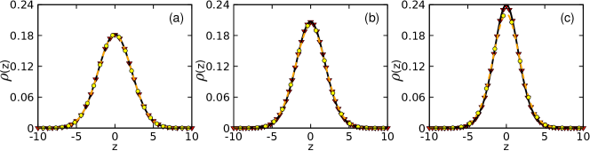
Figure 3: The same as in Fig. (2), but for the self-attractive BEC $(g<0)$, for $g=-0.05$ (a), $g=-0.3$ (b), and $g=-0.5$ (c).

II.1 The YXWLH equation

An effective 1D equation for BEC under the action of the funnel-shaped potential was proposed in Ref. Li et al. (2009), in which the dimensional reduction was performed by means of the VA based on the Gaussian ansatz for the transverse wave function:

$$\psi(r,z,t)=\exp\left(-\frac{r^{2}}{2\eta^{2}}\right)\frac{f(z,t)}{\sqrt{\pi}\delta},$$ (13)

cf. Eq. (7). The effective 1D equation derived in Ref. Li et al. (2009) is

$$i\frac{\partial f}{\partial t}=-\frac{1}{2}\frac{\partial^{2}f}{\partial z^{2}}+V(z)f-\frac{\pi\varepsilon^{6}}{8(1+g|f|^{2})^{2}}f,$$ (14)

which we refer to below as the YXWLH equation. Note that its structure is similar to that of Eq. (12), the difference amounting to replacing coefficient $1/2$ in front of the nonlinear terms by $\pi/8\approx\allowbreak 0.393$. However, no solutions of Eq. (14) were reported in Ref. Li et al. (2009), and the asymptotic structure of the wave function at $r\rightarrow 0$ was not considered either, cf. Eq. (5), the latter point being essential in the case of the singular potential.

II.2 The weak- and strong-nonlinearity cases

For the weakly interacting BEC, with $g|f|^{2}\ll 1,$ Eq. (12) reduces to the usual 1D nonlinear Schrödinger equation (NLSE) with the cubic term,

$$i\frac{\partial f}{\partial t}=-\frac{1}{2}\frac{\partial^{2}f}{\partial z^{2}}+V(z)f-\varepsilon^{6}\left(\frac{1}{2}+g|f|^{2}\right)f.$$ (15)

On the other hand, the Thomas-Fermi (TF) approximation, which neglects the spatial derivatives in the GPEs, may be applied in the case of strong self-repulsion. To this end, we substitute a normalized macroscopic wave function, $\psi(\mathbf{r},t)=\exp\left(-r/2-i\mu t\right)f/\sqrt{2\pi}$, in the 3D GPE (note that this expression corresponds to our initial ansatz (7) with $\eta=1$) and perform the integration in the transverse plane, $(x,y)$, neglecting, as usual, the kinetic-energy terms, the result being

$$|f(z)|^{2}=\begin{cases}{\frac{9}{4g}\left[4\mu-4V(z)+\varepsilon^{3}\right],\,\mathrm{at}\,\mu+\varepsilon^{3}>V(z),}\\ {\newline 0,\,\mathrm{at}\,\mu+\varepsilon^{3}\leq V(z).}\end{cases}$$ (16)

In this approximation, chemical potential $\mu$ is determined by normalization condition (8).

III Numerical results

Numerical results were produced by means of imaginary- and real-time simulations of the full 3D GPE (4), as well as 1D equations (12), (14), and (15). The simulations were performed with the help of the split-step method, that was based on the Crank-Nicolson algorithm. The imaginary-time simulations aimed to produce the system’s GS, while the real-time simulations made it possible to explore dynamical behavior of the models.

We start the analysis of trapped states, predicted by the 3D and 1D equations, adopting the HO potential acting in the axial direction,

$$V(z)=\frac{1}{2}\lambda^{2}z^{2},$$ (17)

with $\lambda^{2}\ll 1$, as the longitudinal potential must be much weaker than its transverse counterpart. To compare the respective GS solutions produced by the 3D and 1D equations, we use the axial-density profile of the 3D state, defined as

$$\rho(z)=\int\int|\psi\left(x,y,z\right)|^{2}dxdy,$$ (18)

while $\rho(z)=|f(z)|^{2}$ for the 1D equations. In Fig. 2, we display typical examples of axial densities for repulsive BEC $(g>0)$ in its GS, under the action of the combined potential (3), in which the longitudinal term is given by Eq. (17) with $\lambda=0.1$. These plots demonstrate that the 1D-NPSE provides essentially more accurate results than other approximations, although Eq. (14), being close to the 1D-NPSE, leads to accuracy which is only slightly worse than provided by the main 1D-NPSE approximation. Thus, it is the best approximation in all cases.

Note that, as observed in Fig. 2, the accuracy of the TF approximation improves slowly with the increase of strength $g$ of the self-repulsion in the underlying GPE (4), while it is usually assumed that the approximation should become better for strong self-repulsion. There are two reasons for that: first, the TF approximation works well with positive confining potentials, such as the OH trap (17), but not necessarily with the singular negative potential, such as the funnel one in Eq. (3); second, the saturable form of Eq. (12) leads to self-cancellation of the strong nonlinearity.

We also analyzed the case of the self-attractive nonlinearity $(g<0)$, under the action of the same combined potential (3). In Fig. 3, we display GS profiles obtained by means of the imaginary-time propagation, applied to the same set of models, viz., the full 3D GPE, 1D-NPSE, 1D-YWLH equation, and cubic 1D-NLSE, while the TF approximation is not relevant in the case of the self-attraction. In this case, all 1D approximations provide good accuracy in comparison with the full 3D findings.

It is well known that the 3D GPE Fibich (2015) and its 1D reductions Salasnich et al. (2002a, b) lead to collapse under the action of a sufficiently strong self-attraction. By means of systematic simulations, we have found that the collapse occurs when the attraction strength exceeds a critical value, $|g|>|g_{c}|$, which is $g_{c}\simeq-0.9$, $g_{c}\simeq-0.8$, and $g_{c}\simeq-0.9$, for the full 3D GPE, 1D-NPSE, and 1D-YXWLH equation, respectively, under the action of the funnel trap (1) with $\varepsilon=1$ and longitudinal potential (17) with $\lambda=0.1$. Although the 1D-NPSE model predicts $g_{c}$ with a slightly poorer accuracy than the 1D-YXWLH equation (14), the comparison of the 1D profiles of the wave functions (not shown here in detail) demonstrates that the former approximation yields better accuracy at $|g|\leq 0.8$.

Getting back to the model with the self-repulsion, in Fig. 4 we display the chemical potential, $\mu$, as obtained numerically from the 3D GPE and from 1D approximations for stationary states, which are looked for, respectively, as $\exp\left(-i\mu t\right)\phi\left(x,y,z\right)$ or $\exp\left(-i\mu t\right)h(z)$, with real functions $\phi$ and $h$, cf. Eq. (5). Again, one observes in Fig. 4 that the 1D-NPSE provides very accurate results [in particular, conspicuously more accurate than those produced by the similar 1D-YXWLH approximate equation (14)].

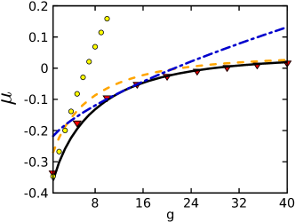
Figure 4: Numerically found chemical potential $\mu$ of the ground state vs. $g$ in the self-repulsive BEC $(g>0)$. Parameters and the notation are the same as in Figs. 2 and 3.

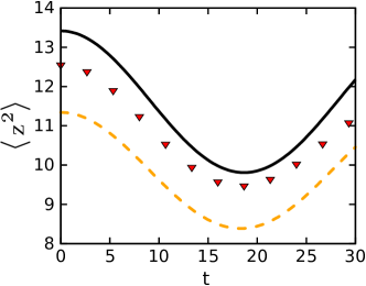
Figure 5: The evolution of the axial mean-squared size $\left\langle z^{2}\right\rangle$ of the dynamical state generated by the quench, i.e., sudden perturbation of the ground-state wave function as per Eq. (19). The self-repulsion coefficient is $g=5$, other parameters and the notation being the same as in Figs. 2-4. The results produced by the simplest approximation, in the form of 1D-NLSE (15), are not displayed here, as their difference form the 3D counterparts is very large.

Finally, we check the accuracy of the 1D-NPSE in simulations of dynamical effects. To this end, we used the input in the form of the GS solutions, which were obtained as outlined above, and ran real-time simulations, suddenly replacing longitudinal potential (17) by a slightly stronger one,

$$V(z)\rightarrow 1.2\times\left(\frac{1}{2}\lambda^{2}z^{2}\right)$$ (19)

(the dynamical behavior of this type is often called quench Dziarmaga (2010)). This variation of the axial confinement gives rise to oscillations of the wave function, which can be observed from the calculation of the axial mean-squared length, $\langle z^{2}\rangle\equiv\int z^{2}|\psi(\mathbf{r})|^{2}d\mathbf{r}$ for 3D GPE, and $\langle z^{2}\rangle\equiv\int_{-\infty}^{+\infty}z^{2}|f|^{2}dz$ for the 1D approximations. In Fig. 5 we compare the evolution of $\langle z^{2}\rangle$ as obtained from the simulations of the full 3D GPE and its 1D counterparts. It is again concluded that the 1D-NPSE is more accurate in comparison with the other approximations. Note that the simplest cubic model, based on 1D-NLSE, i.e., Eq. (15), is very inaccurate in the application to dynamical effects, therefore the respective results are not included in Fig. 5.

Lastly, in the case of self-repulsion, $g>0$, Eq. (12) without the axial potential, $V(z)=0$, generates dark solitons. With this form of the saturable nonlinearity, solutions for dark solitons where found in an exact but cumbersome analytical form in Ref. Krolikowski and Luther-Davies (1993). The comparison of those solutions to their counterparts which may be produced by the 3D equation (2) is a subject for a separate work.

IV Conclusion

In this work, by applying the dimensional-reduction method, which is based on the VA (variational approximation), to the full three-dimensional GPE, we have derived an effective 1D-NPSE (nonpolynomial Schrödinger equation with rational nonlinearity) that governs the axial mean-field dynamics of BEC which is tightly trapped in the transverse plane, with both repulsive and attractive signs of the self-interaction. We have considered the specific case when the transverse trapping is imposed by the singular funnel potential, which is a singular one, $\sim-1/r$. This potential was originally introduced, as a model one, in Ref. Li et al. (2009). We propose physical settings which give rise to this model, viz., a uniformly charged axial wire attracting particles carrying a permanent dipole electric moment, as well as a bosonic gas of magnetic atoms pulled to the axial electric current. In spite of the singularity, the funnel potential maintains regular wave functions of the trapped states. We verify the accuracy of predictions provided by the 1D-NPSE by comparing them to results of the full 3D simulations, and other 1D approximations, such as the usual cubic one-dimensional NLSE and the Thomas–Fermi approximation. In the case of self-attraction ($g<0$), the setting gives rise to collapse at $|g|>\left|g_{c}\right|$, with the critical value also accurately predicted by the 1D reduction. Finally, the 1D-NPSE also provides a sufficiently accurate approximation for dynamical regimes, initiated by a sudden quench applied to the axial potential. Thus, the approximation based on the 1D equation of the NPSE type is relevant for various types of the transverse trapping potentials, including singular ones, and for the analysis of both the systems’ ground states and dynamical regimes.

Finally, it may be interesting to generalize the above analysis for modes with embedded vorticity $S=1,2,3,...$, represented by factor $\exp\left(iS\theta\right)$ in the 3D solution, where $\theta$ is the angular variable in the transverse plane Salasnich et al. (2007c). Then, the expansion similar to that in Eq. (5) starts with terms $\psi=\exp\left(-i\mu t+iS\theta\right)r^{S}\left\{\left[1-\varepsilon^{3}\left(1+2S\right)^{-1}r\right]\psi_{0}(z)+...\right\}$. This extension of the analysis will be reported elsewhere.

References

- Anderson et al. (1995) M. H. Anderson, J. R. Ensher, M. R. Matthews, C. E. Wieman, and E. A. Cornell, Science 269, 198 (1995).
- Davis et al. (1995) K. B. Davis, M. O. Mewes, M. R. Andrews, N. J. van Druten, D. S. Durfee, D. M. Kurn, and W. Ketterle, Physical Review Letters 75, 3969 (1995).
- Bradley et al. (1997) C. C. Bradley, C. A. Sackett, and R. G. Hulet, Phys. Rev. Lett. 78, 985 (1997).
- Griesmaier et al. (2005) A. Griesmaier, J. Werner, S. Hensler, J. Stuhler, and T. Pfau, Phys. Rev. Lett. 94, 160401 (2005).
- Fried et al. (1998) D. G. Fried, T. C. Killian, L. Willmann, D. Landhuis, S. C. Moss, D. Kleppner, and T. J. Greytak, Physical Review Letters 81, 3811 (1998).
- Aikawa et al. (2012) K. Aikawa, A. Frisch, M. Mark, S. Baier, A. Rietzler, R. Grimm, and F. Ferlaino, Phys. Rev. Lett. 108, 210401 (2012).
- Jochim et al. (2003) S. Jochim, M. Bartenstein, A. Altmeyer, G. Hendl, S. Riedl, C. Chin, J. H. Denschlag, and R. Grimm, Science 302, 2101 (2003).
- Zwierlein et al. (2003) M. W. Zwierlein, C. A. Stan, C. H. Schunck, S. M. F. Raupach, S. Gupta, Z. Hadzibabic, and W. Ketterle, Phys. Rev. Lett. 91, 250401 (2003).
- Burger et al. (1999) S. Burger, K. Bongs, S. Dettmer, W. Ertmer, K. Sengstock, A. Sanpera, G. V. Shlyapnikov, and M. Lewenstein, Physical Review Letters 83, 5198 (1999).
- Denschlag et al. (2000) J. Denschlag, J. E. Simsarian, D. L. Feder, C. W. Clark, L. A. Collins, J. Cubizolles, L. Deng, E. W. Hagley, K. Helmerson, W. P. Reinhardt, S. L. Rolston, B. I. Schneider, and W. D. Phillips, Science 287, 97 (2000).
- Khaykovich et al. (2002) L. Khaykovich, F. Schreck, G. Ferrari, T. Bourdel, J. Cubizolles, L. D. Carr, Y. Castin, and C. Salomon, Science 296, 1290 (2002).
- Strecker et al. (2002) K. E. Strecker, G. B. Partridge, A. G. Truscott, and R. G. Hulet, Nature 417, 150 (2002).
- Matthews et al. (1999) M. R. Matthews, B. P. Anderson, P. C. Haljan, D. S. Hall, C. E. Wieman, and E. A. Cornell, Physical Review Letters 83, 2498 (1999).
- Madison et al. (2000) K. W. Madison, F. Chevy, W. Wohlleben, and J. Dalibard, Physical Review Letters 84, 806 (2000).
- Malomed (2019) B. A. Malomed, (2019), arXiv:1904.12081 .
- Inouye et al. (1998) S. Inouye, M. R. Andrews, J. Stenger, H.-J. Miesner, D. M. Stamper-Kurn, and W. Ketterle, Nature 392, 151 (1998).
- Petrov (2015) D. S. Petrov, Physical Review Letters 115, 155302 (2015).
- Petrov and Astrakharchik (2016) D. S. Petrov and G. E. Astrakharchik, Physical Review Letters 117, 100401 (2016).
- Cabrera et al. (2018) C. R. Cabrera, L. Tanzi, J. Sanz, B. Naylor, P. Thomas, P. Cheiney, and L. Tarruell, Science 359, 301 (2018).
- Cheiney et al. (2018) P. Cheiney, C. R. Cabrera, J. Sanz, B. Naylor, L. Tanzi, and L. Tarruell, Physical Review Letters 120, 135301 (2018).
- Semeghini et al. (2018) G. Semeghini, G. Ferioli, L. Masi, C. Mazzinghi, L. Wolswijk, F. Minardi, M. Modugno, G. Modugno, M. Inguscio, and M. Fattori, Physical Review Letters 120, 235301 (2018).
- Ferioli et al. (2019) G. Ferioli, G. Semeghini, L. Masi, G. Giusti, G. Modugno, M. Inguscio, A. Gallemí, A. Recati, and M. Fattori, Physical Review Letters 122, 090401 (2019).
- D’Errico et al. (2019) C. D’Errico, A. Burchianti, M. Prevedelli, L. Salasnich, F. Ancilotto, M. Modugno, F. Minardi, and C. Fort, (2019), arXiv:1908.00761 .
- Pitaevskii and Stringari (2003) L. P. Pitaevskii and S. Stringari, Bose-Einstein Condensation, International Series of Monographs on Physics (Clarendon Press, 2003).
- Pethick and Smith (2008) C. J. Pethick and H. Smith, Bose-Einstein Condensation in Dilute Gases (Cambridge University Press, Cambridge, 2008).
- Muryshev et al. (2002) A. Muryshev, G. V. Shlyapnikov, W. Ertmer, K. Sengstock, and M. Lewenstein, Physical Review Letters 89, 110401 (2002).
- Salasnich et al. (2002a) L. Salasnich, A. Parola, and L. Reatto, Physical Review A 65, 043614 (2002a).
- Salasnich et al. (2002b) L. Salasnich, A. Parola, and L. Reatto, Physical Review A 66, 043603 (2002b).
- Massignan and Modugno (2003) P. Massignan and M. Modugno, Physical Review A 67, 023614 (2003).
- Kamchatnov and Shchesnovich (2004) A. M. Kamchatnov and V. S. Shchesnovich, Physical Review A 70, 023604 (2004).
- Carr and Brand (2004) L. D. Carr and J. Brand, Physical Review Letters 92, 040401 (2004).
- Zhang and You (2005) W. Zhang and L. You, Physical Review A 71, 025603 (2005).
- Salasnich and Malomed (2006) L. Salasnich and B. A. Malomed, Physical Review A 74, 053610 (2006).
- Matuszewski Michałand Królikowski et al. (2006) W. Matuszewski Michałand Królikowski, M. Trippenbach, Y. S. Kivshar, M. Matuszewski, W. Królikowski, M. Trippenbach, Y. S. Kivshar, W. Matuszewski Michałand Królikowski, M. Trippenbach, and Y. S. Kivshar, Phys. Rev. A 73, 63621 (2006).
- Wei et al. (2007) P. Wei, L. Zhi-Bing, and B. Cheng-Guang, Chinese Physics Letters 24, 2745 (2007).
- Salasnich et al. (2007a) L. Salasnich, A. Cetoli, B. A. Malomed, F. Toigo, and L. Reatto, Physical Review A 76, 013623 (2007a).
- Salasnich et al. (2007b) L. Salasnich, A. Cetoli, B. A. Malomed, and F. Toigo, Physical Review A 75, 033622 (2007b).
- Mateo and Delgado (2007) A. M. Mateo and V. Delgado, Physical Review A 75, 063610 (2007).
- Maluckov et al. (2008) A. Maluckov, L. Hadžievski, B. A. Malomed, and L. Salasnich, Physical Review A 78, 013616 (2008).
- Salasnich et al. (2008) L. Salasnich, B. A. Malomed, and F. Toigo, Physical Review A 77, 035601 (2008).
- Salasnich (2009) L. Salasnich, Journal of Physics A: Mathematical and Theoretical 42, 335205 (2009).
- Li et al. (2009) Y. Li, X. Guang-Yuan, W. Yong-Jun, L. Xian-Feng, and H. Jiu-Rong, Communications in Theoretical Physics 52, 431 (2009).
- Buitrago and Adhikari (2009) C. A. G. Buitrago and S. K. Adhikari, Journal of Physics B: Atomic, Molecular and Optical Physics 42, 215306 (2009).
- Adhikari and Salasnich (2009) S. K. Adhikari and L. Salasnich, New Journal of Physics 11, 023011 (2009).
- Salasnich and Malomed (2009) L. Salasnich and B. A. Malomed, Physical Review A 79, 053620 (2009).
- Muñoz Mateo and Delgado (2009) A. Muñoz Mateo and V. Delgado, Annals of Physics 324, 709 (2009).
- Young-S. et al. (2010) L. E. Young-S., L. Salasnich, and S. K. Adhikari, Physical Review A 82, 053601 (2010).
- Cardoso et al. (2011) W. B. Cardoso, A. T. Avelar, and D. Bazeia, Physical Review E 83, 036604 (2011).
- Mateo et al. (2011) A. M. Mateo, V. Delgado, and B. A. Malomed, Physical Review A 83, 053610 (2011).
- Edwards et al. (2012) M. Edwards, M. Krygier, H. Seddiqi, B. Benton, and C. W. Clark, Physical Review E 86, 056710 (2012).
- Díaz et al. (2012) P. Díaz, D. Laroze, I. Schmidt, and B. A. Malomed, Journal of Physics B: Atomic, Molecular and Optical Physics 45, 145304 (2012).
- Salasnich and Malomed (2013) L. Salasnich and B. A. Malomed, Physical Review A 87, 063625 (2013).
- Salasnich et al. (2014) L. Salasnich, W. B. Cardoso, and B. A. Malomed, Physical Review A 90, 033629 (2014).
- Chiquillo (2015) E. Chiquillo, Journal of Physics A: Mathematical and Theoretical 48, 475001 (2015).
- dos Santos and Cardoso (2019) M. C. P. dos Santos and W. B. Cardoso, Phys. Lett. A 383, 250401 (2019).
- Cuevas et al. (2013) J. Cuevas, P. G. Kevrekidis, B. A. Malomed, P. Dyke, and R. G. Hulet, New Journal of Physics 15, 063006 (2013).
- De Nicola et al. (2006) S. De Nicola, B. A. Malomed, and R. Fedele, Physics Letters A 360, 164 (2006).
- Li et al. (2017) Y. Li, Z. Luo, Y. Liu, Z. Chen, C. Huang, S. Fu, H. Tan, and B. A. Malomed, New Journal of Physics 19, 113043 (2017).
- Li et al. (2018) Y. Li, Z. Chen, Z. Luo, C. Huang, H. Tan, W. Pang, and B. A. Malomed, Physical Review A 98, 063602 (2018).
- Sakaguchi and Malomed (2011) H. Sakaguchi and B. A. Malomed, Physical Review A 83, 013607 (2011).
- Denschlag and Schmiedmayer (1997) J. Denschlag and J. Schmiedmayer, Europhysics Letters (EPL) 38, 405 (1997).
- Ferrier-Barbut et al. (2016) I. Ferrier-Barbut, H. Kadau, M. Schmitt, M. Wenzel, and T. Pfau, Physical Review Letters 116, 215301 (2016).
- Schmitt et al. (2016) M. Schmitt, M. Wenzel, F. Böttcher, I. Ferrier-Barbut, and T. Pfau, Nature 539, 259 (2016).
- Chomaz et al. (2016) L. Chomaz, S. Baier, D. Petter, M. J. Mark, F. Wächtler, L. Santos, and F. Ferlaino, Physical Review X 6, 041039 (2016).
- Fibich (2015) G. Fibich, The Nonlinear Schrödinger Equation: Singular Solutions and Optical Collapse, Applied Mathematical Sciences, Vol. 192 (Springer International Publishing, Cham, 2015).
- Dziarmaga (2010) J. Dziarmaga, Advances in Physics 59, 1063 (2010).
- Krolikowski and Luther-Davies (1993) W. Krolikowski and B. Luther-Davies, Optics Letters 18, 188 (1993).
- Salasnich et al. (2007c) L. Salasnich, B. A. Malomed, and F. Toigo, Physical Review A 76, 063614 (2007c).