Quantum Hall criticality in Floquet topological insulators

Abstract

The anomalous Floquet Anderson insulator (AFAI) is a two dimensional periodically driven system in which static disorder stabilizes two topologically distinct phases in the thermodynamic limit. The presence of a unit-conducting chiral edge mode and the essential role of disorder induced localization are reminiscent of the integer quantum Hall (IQH) effect. At the same time, chirality in the AFAI is introduced via an orchestrated driving protocol, there is no magnetic field, no energy conservation, and no (Landau level) band structure. In this paper we show that in spite of these differences the AFAI topological phase transition is in the IQH universality class. We do so by mapping the system onto an effective theory describing phase coherent transport in the system at large length scales. Unlike with other disordered systems, the form of this theory is almost fully determined by symmetry and topological consistency criteria, and can even be guessed without calculation. (However, we back this expectation by a first principle derivation.) Its equivalence to the Pruisken theory of the IQH demonstrates the above equivalence. At the same time it makes predictions on the emergent quantization of transport coefficients, and the delocalization of bulk states at quantum criticality which we test against numerical simulations.

I Introduction

Topological Floquet insulators (TFI) are gapped quantum systems with topological structures generated by a periodic drive. The material class includes conventional topological insulators subject to external driving Oka and Aoki (2009); Lindner and Refael (2011), quantum walks Kitagawa et al. (2012); Edge and Asboth (2015), periodically kicked matter Dahlhaus et al. (2011); Tian et al. (2016), driven Anderson insulatorsTitum et al. (2016), and others Jiang et al. (2011); Rechtsman et al. (2013); Potirniche et al. (2017); Higashikawa et al. (2019). TFIs share many observable properties with static topological insulators. Specifically, they feature phases with quantized edge modes which are protected by a gapped bulk and separated from trivial phases via gap closing transitions. However, these analogies notwithstanding, the physics of topological protection in Floquet quantum matter is based on principles quite different from those in static systemsKitagawa et al. (2010); Rudner et al. (2013); Roy and Harper (2017).

To see why, recall that the topological invariants of a static topological insulator describe twists in its free fermion ground state Kitaev (2009). The identity of the latter is protected by a spectral gap, or an excitation gap, in the presence of disorder. However, absent energy conservation, topological order in a Floquet system cannot be based on features of individual of its (quasi–)energy bands. Any topological classification must address the totality of all Floquet eigenstates, which is information equivalent to the Floquet operator, $\hat{U}$, itself. For example, in systems void of time-reversal and/or charge-conjugation symmetry (class A), the Floquet operator $\hat{U}\in\mathrm{U}(N)$ is just an $N$-dimensional unitary matrix, and topological invariants must be described via those supported by $\mathrm{U}(N)$. This brings about the seemingly paradoxical situation that there do exist class A TFIs in two-dimensional space Rudner et al. (2013), while the unitary group in two dimensions is topologically empty. (Invariants for the unitary group exist only in odd–dimensional parameter spaces.)

It has been understood Titum et al. (2016) that the resolution of this conundrum lies in the stabilization of topological phases by disorder. At first sight, this may seem counterintuitive: the addition of weak disorder to a clean system removes band gaps and leads to the hybridization of surface states with spatially extended bulk states (According to Mott’s criterion energetically degenerate localized and extended states cannot coexist) compromising the identity of the latter. However, the situation changes in the thermodynamic limit, where disorder induced localization renders the bulk fully insulating, which leads to surface state protection in full analogy to the conspiracy of localization and topology in the integer quantum Hall (IQH) effect. This argument indicates that topological invariants in topological Floquet matter are emergent invariants which become well defined only in the thermodynamic limit. Intuitively, the scaling parameter controlling the size of the system provides the third parameter required to define an invariant for $\mathrm{U}(N)$.

As a corollary, the phase transitions between different topological sectors must be Anderson localization/delocalization transitions. In static two-dimensional systems lacking symmetries besides unitarity we know only one topological Anderson transition, the IQH transition. This raises the question for the universality class of the TFI phase transition in two-dimensions, is it in the IQH class, or not? Arguments in either direction may be put forward. On the one hand, it seems natural that an Anderson transition between phases with different chiral edge modes should be intimately related to the IQH transition. On the other hand, the absence of energy conservation and of a bulk Landau level structure (with delocalized Landau level centers deep below the Fermi surface) point in a different direction.

All these questions can be addressed on the example of the AFAI, a beautiful paradigm of two-dimensional topological Floquet quantum matter introduced in Ref. Rudner et al. (2013). In this paper, we will present a first principle theory of this TFI subject to maximally strong disorder. We will provide analytical evidence backed by numerical observation that the system is in the IQH universality class. The general strategy of our approach, a mapping of the microscopic theory to an effective theory describing its physics at large length and time scales, carries over to other forms of topological Floquet quantum matter, both insulating and gapless. A central message of this approach is that, unlike in the physics of topological band insulators, the presence of disorder is key to the stabilization of topological phases in Floquet matter. The ensuing ensemble averaged theories, are simple and depend only on few (two in general) system parameters characterizing the interplay of bulk localization and topology. We will discuss how the flow of these couplings reflects in microscopic observables and apply exact diagonalization to probe the critical regime and compare to the predictions of the effective theory.

The rest of the paper is organized as follows. After a brief review of the AFAI in section II we discuss its effective theory in section III. As stated above, this will be done on the basis of consistency reasoning (no previous knowledge in the field theory of disordered systems is required to follow this construction). In section IV we discuss the connection between the effective theory and observables and put this connection to a numerical test. Finally, in section V (optional reading) we show how the effective theory is derived from first principles. Our technical calculations are relegated to few Appendices.

II AFAI

The AFAI is a two dimensional driven disordered system displaying a topological phase transition Rudner et al. (2013). It is defined via a five-step driving protocol on a two-dimensional square lattice (cf. Fig. 1 a)): $U_{d}\equiv UU_{\phi}\equiv U_{4}U_{3}U_{2}U_{1}U_{\phi}$. Here, the unitary operators $U_{1,2,3,4}$ describe deterministic nearest neighbor directed hopping along the bonds of the lattice, represented in a 45^∘ rotated orientation in Fig. 1 to conveniently describe the ($A/B$) unit cell structure crucial to the definition of the theory. In momentum space these four operators read

$$U_{i}(\mathbf{k}) =\exp\bigl{(}itV_{i}(\mathbf{k})\bigr{)}=\cos(t)+i\sin(t)V_{i}(\mathbf{k}),$$ (1)

$$V_{i}(\mathbf{k})=\left(\begin{matrix}&e^{-i\mathbf{k}\cdot\mathbf{v}_{i}}\cr e^{i\mathbf{k}\cdot\mathbf{v}_{i}}\end{matrix}\right),$$ (2)

where the matrix structure is in ($A/B$) – space and the definition of the hopping vectors, $\mathbf{v}_{i}$, follows from inspection of the figure as $(\mathbf{v}_{1},\mathbf{v}_{2},\mathbf{v}_{3},\mathbf{v}_{4})=(0,-\mathbf{e}_{1},-\mathbf{e}_{1}+\mathbf{e}_{2},\mathbf{e}_{2})$ with $\mathbf{e}_{1,2}$ being lattice unit vectors in the horizontal/vertical direction. The dimensionless parameter $t$ determines the amplitude of the hopping, interpolating between a stationary limit, $t=0$, and hopping with unit probability, $t=\pi/2$. Finally, a site diagonal operator

$$U_{\phi}(\mathbf{x})\equiv\left(\begin{matrix}e^{i\phi_{A}(\mathbf{x})}&\cr&e^{i\phi_{B}(\mathbf{x})}\end{matrix}\right)$$ (3)

introduces disorder as random phases at the lattice points. We here consider the case of maximal disorder, where $e^{i\phi_{A/B}(\mathbf{x})}$ at the lattice sites $\mathbf{x}=(x_{1},x_{2})$ are independently and identically distributed over the unit circle (Fig. 1, c)).

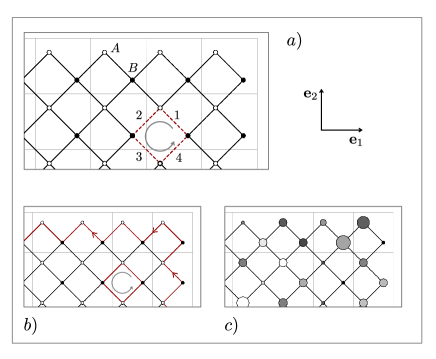
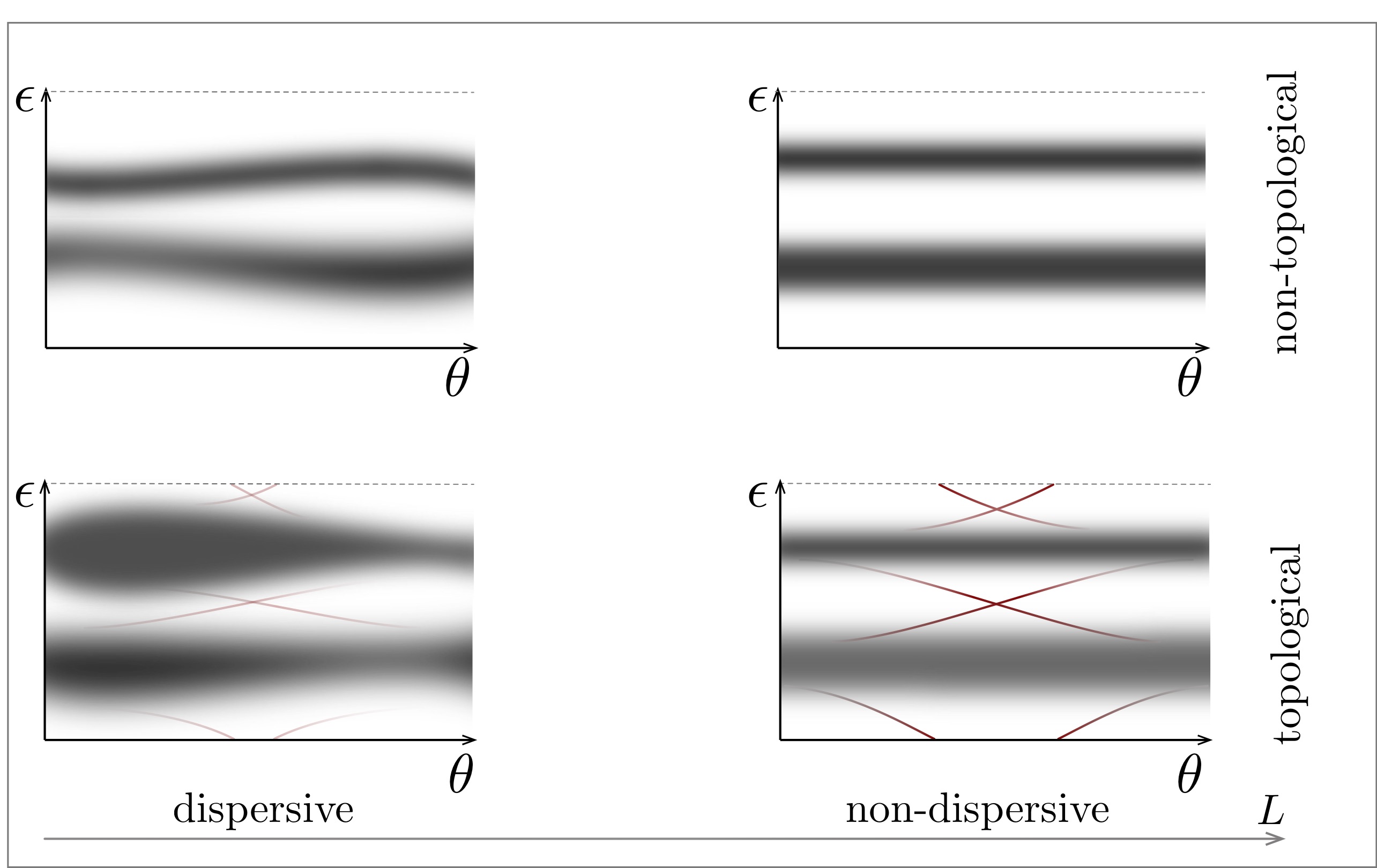
Figure 1: Top: a) four step driving protocol for sequential hopping around the plaquettes of a square lattice with tunable amplitude, $t$. b) Edge mode in the limit of unit probability hopping. c) Application of site diagonal disorder in the initial step. Bottom: schematic of the sensitivity of the Floquet quasi energy spectrum to changes in boundary conditions. Left: for finite system sizes the spectrum contains quasi-energy bands, whose dispersiveness diminishes upon increasing system size. In a pre-topological regime, the precursors of a chiral mode are formed. Right: in the thermodynamic limit, bulk modes have become non-dispersive, indicating complete localization. In addition to that, the spectrum contains a robust chiral edge mode.

The presence of topology in the system is understood by inspection of two limiting cases: for $t=0$ there is no hopping at all, and the clean part of the Floquet operator, $U\equiv\prod_{i=1}^{4}U_{i}$ reduces to the unit operator. By contrast, for $t=\pi/2$, we have hopping with unit probability, which means that the bulk $U$, sends particles back to their point of departure and likewise acts as a identity operation. However, in this case, the inert bulk is surrounded by an edge mode encircling the system in counter clockwise direction (Fig. 1, b)).

Crucially, however, the two points $t=0,\pi$ do not define topological phases of the clean system. Any perturbation away from these configurations, introduces bulk extended states, hybridizing the boundaries and compromising their chiral edge mode. The definition of perturbatively robust phases requires the stabilizing influence of disorder. Disordered two dimensional systems in class A are subject to Anderson localization. To anticipate its interplay with a topological phase, we consider a gedanken experiment where twisted boundary conditions specified by an angle $\theta$ in, say, $x$-direction are applied. For a system of finite size, $L$, generic states will respond to changes in the boundary conditions, thus rendering the set of quasi-energy levels dispersive under variations of $\theta$ (Fig. 1) left. For $t$ closer to $\pi/2$ than to $0$, signatures of edge modes, still compromised by bulk hybridization begin to form (bottom left). In the thermodynamic limit, all bulk bands have become flat, indicating complete localization. At the same time, two chiral edge modes, counter propagating at the upper and lower edge have formed. The stabilization of the edge modes and the non-dispersiveness of the bulk are flip sides of the same coin. This scenario indicates that the essential physics of the system is encoded in the flow of two parameters, a bulk transport coefficient, $g(L)$, and a topological index $\chi(L)$. For generic bare values $(g_{0},\chi_{0})$, one expects flow $(g_{0},\chi_{0})\stackrel{{\scriptstyle L\rightarrow\infty}}{{\longrightarrow}}(0,n)$, where $n=0,1$ depending on $\chi_{0}$. These variants must be separated by a critical surface, $g_{0},\chi_{\mathrm{crit}}$, where bulk states remain delocalized.

III Effective theory

To better understand the physics outline above, an effective theory of the disordered system is needed. The latter must contain structures defined in crystal momentum space, where $U=U(\mathbf{k})$ describes the clean system, and in real space, where the physics of localization develops. In this paper, we discuss how such a theory is derived from first principles by methods previously developed for other problems with random unitary operators Zirnbauer (1996); Altland et al. (2015). This construction reveals differences and analogies to the localization theory of the IQH effect, and shows how the flowing coupling constants entering the effective theory are related to response functions which can be measured, e.g., by numerical experiments.

In this paper, we offer two avenues to the construction of the theory. In this section, it is ‘derived’ on the basis of symmetry reasoning, and a few references to general elements of localization theory. The present system is special in that such reasoning is sufficient to almost fully determine its effective long range theory. In particular, the structure of the topological terms governing the disordered system can be understood in this way. In section V, interested readers find an alternative derivation of the theory which is more technical and based on a first principle construction.

We first note that all information required to describe transport and topological properties of the system is contained in the retarded and advanced ‘resolvents’,

$$G^{+}(\phi)\equiv\frac{1}{1-e^{-\delta}e^{i\phi}U_{\mathrm{d}}},\quad G^{-}(\phi)\equiv\frac{1}{1-e^{-\delta}e^{-i\phi}U^{\dagger}_{\mathrm{d}}},$$ (4)

where $\delta\to 0^{+}$. For example, in Appendix A, we show that the Floquet Hall coefficient probing transverse response is given by the sum of two terms, $\widetilde{\sigma}_{H}=\sigma^{\rm I}+\sigma^{\rm II}$, with

$$\sigma^{\rm I}=-\frac{1}{2A}\epsilon_{ij}\left\langle{\rm tr}\left(v_{i}G^{+}v_{j}G^{-}\right)\right\rangle_{\phi},\quad\sigma^{\rm II}=\frac{1}{2A}\epsilon_{ij}\,{\rm tr}(x_{i}v_{j}),$$ (5)

where $\langle\dots\rangle_{\phi}=\int_{0}^{2\pi}\frac{d\phi}{2\pi}(\dots)$ is a quasi-energy average, $A=L_{1}L_{2}$ is the system area, we have defined $G^{\pm}\equiv G^{\pm}(0)$, and

$$v_{i}\equiv x_{i}^{U}\equiv Ux_{i}U^{\dagger}-x_{i},$$ (6)

is the Floquet analog of the velocity operator in an Hamiltonian system. (The analogy is seen by writing $U=\exp(itH)$ and considering the limit of short stroboscopic time: $x^{U}_{i}\to i[H,x_{i}]=\partial_{k_{i}}H=v_{i}$  .) Physically, the matrix elements $G^{+}_{\mu\nu}(\phi,\mathbf{y},\mathbf{x})\equiv\langle\mu,\mathbf{y}|G^{+}(\phi)|\nu,\mathbf{x}\rangle$ with $\mu,\nu\in\{A,B\}$ referring to the sublattice structure, describe the retarded Floquet evolution of states in the system. This is best seen in a discrete time Fourier transform representation $G^{+}(t,\mathbf{y},\mathbf{x})=\int\frac{d\phi}{2\pi}e^{i\phi t}G^{+}(\phi,\mathbf{y},\mathbf{x})=\langle\mathbf{y}|\mathbf{x}^{+}_{t}\rangle$, where $|\mathbf{x}_{t}^{+}\rangle\equiv U_{\mathrm{d}}^{t}|\mathbf{x}\rangle$, $t\in\mathbb{N}^{+}$ is the stroboscopic evolution of an initial localized state $|\mathbf{x}\rangle$ and we omitted sublattice indicies for brevity. In a similar way, $G^{-}$ describes the advanced evolution under $U_{d}^{\dagger t}=U_{d}^{-t}$. The issue with these stroboscopically propagated lattice wave functions is that they are wildly oscillatory. It has been a crucial insight of early localization theory Wegner (1979); Efetov et al. (1980); Pruisken and Schäfer (1982); Efetov and Larkin (1983); Pruisken (1984) that an efficient description of disordered quantum systems should be based on wave function bilinears. The corresponding composite degrees of freedom are the $Q$-matrices of the non-linear $\sigma$-model. Originally introduced within the framework of static disordered systems, their applicability extends to the present context, as demonstrated by explicit construction in section V. We here take the alternative route to introduce these degrees of freedom on the basis of qualitative reasoning:

We define matrices $Q(\mathbf{x})=\{Q^{sa,s^{\prime}a^{\prime}}(\mathbf{x})\}$ carrying a two fold index structure: the first index pair $s,s^{\prime}=\pm$ distinguishes between advanced and retarded degrees of freedom such that

$$Q^{aa^{\prime}}(\mathbf{x})\sim\left(\begin{matrix}|\mathbf{x}^{+}\rangle\langle\mathbf{x}^{+}|&|\mathbf{x}^{+}\rangle\langle\mathbf{x}^{-}|\cr|\mathbf{x}^{-}\rangle\langle\mathbf{x}^{+}|&|\mathbf{x}^{-}\rangle\langle\mathbf{x}^{-}|\end{matrix}\right)^{aa^{\prime}}$$ (7)

represents wave function bilinears of either sense of propagation, retarded or advanced. The meaning of the subscripts is that the time evolution of the $Q$’s is generated by action of powers of $U_{d}$ $(U_{d}^{\dagger})$ on $|\mathbf{x}^{+}\rangle$, ($|\mathbf{x}^{-}\rangle$). Crucially, the ‘adjoint’ action generated by $U_{d}$ and $U_{d}^{\dagger}$ contains contributions where rapid phase oscillations cancel out, which makes $Q$ a candidate for an effective slowly fluctuating variable. For example, in $Q$-language, transport correlation functions are represented as correlation functions of the structure, $\langle\mathbf{x}|G^{+}|\mathbf{y}\rangle\langle\mathbf{y}|G^{-}|\mathbf{x}\rangle\sim\langle Q^{+-}(\mathbf{y})Q^{-+}(\mathbf{x})\rangle_{Q}$, or ‘spectral’ correlation functions as $\langle\mathbf{x}|G^{+}|\mathbf{x}\rangle\langle\mathbf{y}|G^{-}|\mathbf{y}\rangle\sim\langle Q^{++}(\mathbf{x})Q^{--}(\mathbf{y})\rangle_{Q}$, where the averages $\langle\dots\rangle_{Q}$ refer to a $Q$-functional average to be discussed momentarily. The second index, $a,a^{\prime}$ is required by the disorder average. Depending on the chosen method, this can be a replica index $a=1\dots,R$, with an analytic continuation $R\to 0$ at the end, or a ‘super-index’ $a=\mathrm{b,f}$ distinguishing between commuting and anti-commuting components in a supersymmetric approach Efetov (1997). Either way, this structure will not play an essential role in our present discussion, and we choose a replica representation for definiteness.

The $Q$-matrices possess a distinct internal structure which on robust grounds is dictated by unitarity conditions Wegner (1979). A standard representation incorporating these principles reads, $Q=T\tau_{3}T^{-1}$, where $\tau_{3}$ is a Pauli matrix in the representation of Eq. (7), and $T\in\mathrm{U}(2R)$. This structure implies that matrices $T$ commuting with $\tau_{3}$ are irrelevant, which makes $Q$ an element of the coset space $\mathrm{U}(2R)/\mathrm{U}(R)\times\mathrm{U}(R)$. In the single replica case, $R=1$, this is just a two sphere $S^{2}=\mathrm{U}(2)/\mathrm{U}(1)\times\mathrm{U}(1)$. For general $R$, the field manifolds are more complicated, but their geometry, coordinates, etc. still resemble those of generalized spheres.

The theory we are looking for must be described by a simple action for the momentum space degrees of freedom. $U(\mathbf{k})$ and the real space field $Q(\mathbf{x})$. Principles entering the definition of this action include (i) locality, (ii) simplicity (i.e. lowest number of derivatives), (iii) symmetry under ‘canonical’ transformations of the coordinates $\mathbf{x}$ and momenta $\mathbf{k}$, and (iv) internal symmetry. The latter principle requires that, e.g., a change of reference frames $U(\mathbf{k})\to U_{0}U(\mathbf{k})U_{0}^{-1}$, $Q(\mathbf{x})\to T_{0}Q(\mathbf{x})T_{0}^{-1}$ should leave the action invariant. In the following we show that these conditions determine the effective action, up to one inessential numerical constant.

Diffusive action: Condition (iv) above excludes the presence of zero derivative terms, and (iii) that of first order derivative terms in an effective action. To lowest, second order, an obvious candidate compatible with (iii) reads $S_{0}[U]\equiv\int d^{2}k\,\mathrm{tr}(\partial_{i}U\partial_{i}U^{-1})$, where $d^{2}k\equiv dk_{1}dk_{2}/(2\pi)^{2}$ and $\partial_{i}\equiv\partial_{k_{i}}$. Notice, however, that this term cannot appear on its own in a valid effective action. The reason is that the (canonical) scale transformation $k_{i}\to b_{i}k_{i}$, $x_{i}\to b^{-1}_{i}x_{i}$ does not leave it invariant. The natural $Q$-partner for pairing reads $S_{0}[Q]\equiv\int d^{2}x\,\mathrm{tr}(\partial_{i}Q\partial_{i}Q)$, where $d^{2}x=dx_{1}dx_{2}$, and $\partial_{1,2}\equiv\partial/\partial x_{1,2}$. The product $S_{\mathrm{diff}}[Q,U]\equiv S_{0}[U]S_{0}[Q]$ satisfies all criteria listed above. Seen as a real space action it defines

$$S_{\mathrm{diff}}[Q] \equiv{\sigma^{(0)}_{11}\over 8}\int d^{2}x\,\mathrm{tr}(\partial_{i}Q\partial_{i}Q),$$ (8)

$$\sigma^{(0)}_{11} \equiv\frac{1}{2}\int d^{2}k\,\mathrm{tr}(\partial_{1}U\partial_{1}U^{-1}).$$ (9)

where, the coupling constant $\sigma^{(0)}_{11}$ defines the mobility of the system at the bare level.

Within the $\sigma$-model approach, the conduction properties of disordered metals Wegner (1979) are described by a term of identical structure. In that context, the coupling constant plays the role of the longitudinal conductance (in units of the conductance quantum $\mathrm{e}^{2}/h$), which motivates the denotation $\sigma_{11}$. In the present context, a straightforward calculation yields $\sigma^{(0)}_{11}(t)=\tfrac{1}{2}\sin^{2}2t$ (see Fig. 2). As expected, the mobility approaches zero in the limiting cases of none and unit probability hopping around the lattice plaquettes, respectively. At $t=\pi/4$, a maximum value $\sigma_{11}^{(0)}=1/2$, corresponding to a half of the conductance quantum is reached.

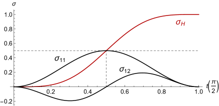
Figure 2: Coupling constants of the nonlinear $\sigma$-model action as a function of $t$ (in units $\pi/2$). At $t=\pi/4$ the system passes through a critical point characterized by a half integer quantized value of $\sigma_{H}$ and a maximum of $\sigma_{11}$.

Topological action: In addition to principles (i-iv), a topological action must satisfy (v), independence of a metric. In combination with the other principles above this means that both the real space and the momentum space topological action must be insensitive to coordinate transformations. Beginning with the real space sector, we temporarily assume periodic boundary conditions, such that $\mathbf{x}\in T^{2}$ becomes the coordinate of a 2-torus. For $R=1$, $Q$ lives on a sphere, and $Q(\mathbf{x})$ defines a map from the torus to the sphere which can be classified by winding numbers. For example, using the parameterization, $Q=n_{a}\tau_{a}$ with $|\mathbf{n}|=1$, this invariant is obtained by the familiar surface integral $\frac{1}{8\pi}\epsilon^{abc}\int d^{2}x\epsilon^{ij}n_{a}\partial_{i}n_{b}\partial_{j}n_{c}\equiv W\in\mathbb{Z}$. The generalization of this expression to arbitrary $R$ reads $iS_{\theta}[Q]\equiv\frac{1}{16\pi}\int d^{2}x\,\epsilon^{ij}\,\mathrm{tr}(Q\partial_{i}Q\partial_{j}Q)$. This integral determines the homotopy class of the map $T^{2}\to\mathrm{U}(2R)/\mathrm{U}(R)\times\mathrm{U}(R),\mathbf{x}\mapsto Q(\mathbf{x})$.

Turning to the conjugate degree of freedom $U(\mathbf{k})$, the unique topological action definable over a two-dimensional parameter space is the Wess-Zumino-Witten (WZW) term

$$\Gamma[U]\equiv-\frac{1}{12\pi}\int d^{3}k\,\epsilon^{\mu\nu\sigma}\mathrm{tr}(U^{-1}\partial_{\mu}UU^{-1}\partial_{\nu}UU^{-1}\partial_{\sigma}U).$$ (11)

Here, $k=\{k_{\mu}\}\equiv(s,k_{1},k_{2})$ is a three-dimensional vector, containing a parameter $s$ as the zeroth component. We define $U(k)\equiv U(s,\mathbf{k})$ as a matrix obtained by generalization $t\to s$ in Eq. (1). In this way, $U(0,\mathbf{k})=\mathds{1}$, and $U(t,\mathbf{k})=U(\mathbf{k})$, i.e. $s$ is a homotopy parameter, such that $U(s,\mathbf{k})$ interpolates between the unit matrix and $U(\mathbf{k})$. The $s$-integration in the definition of $\Gamma[U]$ extends over the interpolation interval, $\int_{0}^{t}ds$.

Geometrically, $\Gamma[U]$ is the three dimensional volume swept out by the map $U(s,\mathbf{k})$ in $\mathrm{U}(2)$, where the latter is defined to cover the interpolation between $\mathds{1}$ and $U(\mathbf{k})$. However, there is an ambiguity in this construction Altland and Simons (2010): instead of interpolating to $\mathds{1}$, one could have chosen $-\mathds{1}$ as the anchor point. This would have led to a different functional $\tilde{\Gamma}[U]$. This choice, which has a status similar to a gauge ambiguity, must be physically inconsequential. As with the physically equivalent Dirac spin quantization condition, the solution is to require that $\Gamma[U]$ couples to the action via a coupling constant, $\exp(i\kappa\Gamma[U])$ such that $\exp(i\kappa(\Gamma[U]-\tilde{\Gamma}[U]))=1$. By construction, $\Gamma[U]-\tilde{\Gamma}[U]$ equals the integral over the full unitary group, which in the present normalization equals $2\pi$. This argument shows that the coupling constants, $\kappa$, by which a WZW term enters the action must be integer quantized.

Above we have seen, that the topological action $iS_{\theta}[Q]\equiv W$ is integer quantized. This makes the hybrid $S_{\mathrm{top}}[Q,U]\equiv\Gamma[U]S_{\theta}[Q]$ the unique topological action consistent with all criteria, (i-v). Emphasizing the real space part, this reads

$$S_{\mathrm{top}}[Q] \equiv\frac{\sigma^{(0)}_{H}}{8}\int d^{2}x\,\epsilon^{ij}\,\mathrm{tr}(Q\partial_{i}Q\partial_{j}Q),$$ (12)

$$\sigma^{(0)}_{H} \equiv\frac{1}{2\pi}\Gamma[U].$$ (13)

Here, $\sigma^{(0)}_{H}$ is the antisymmetric contribution to the Hall conductivity, labeled by the subscript ‘$H$’ to distinguish it from the symmetric $\sigma_{12}$ defined above. For the Floquet of Eq. (1), a straightforward computation shows that $\Gamma[U]=2\pi(1+2\cos^{2}t)\sin^{4}t$. Specifically, at $t\equiv t_{\mathrm{crit}}=\pi/4$, $\sigma^{(0)}_{H}=1/2$. As we are going to discuss next, this marks the quantum phase transition of the system.

Quantum Hall criticality: The action $S[Q]=S_{\mathrm{diff}}[Q]+S_{\mathrm{top}}[Q]$ equals the Pruisken action Pruisken (1984) for the IQH. We need to caution, though, that the derivation of the Pruisken action of the IQH is parametrically controlled by the assumption of weak disorder (meaning a large dimensionless product of Fermi energy and scattering time), which translates to large values of the longitudinal coupling $\sigma^{(0)}_{11}$. In the present problem, the bare value $\sigma^{(0)}_{11}=\mathcal{O}(1)$ means that the model is derived in a strong coupling regime, where the fields $Q$ strongly fluctuate, and the limitation to terms with two derivatives is no longer parametrically controlled. While higher order terms are renormalization group irrelevant, the assumption of stability of the action is not quite innocent, as we know that the IQH critical point itself is described by a conformal field theory different from the Pruisken model and whose identity is the subject of ongoing research Zirnbauer (2019); Bondesan et al. (2017). Strictly speaking, it is a matter of believe, backed by the numerical evidence presented in subsection IV.3, that the action $S[Q]$ correctly describes the system, including at strong disorder.  (For completeness, we mention that for weak disorder the identity of individual of the Chern quasi–energy bands of the clean AFAI remains visible Rudner and Lindner (2019). This may well lead to more complicated physics, beyond the scope of the present analysis.)

A renormalization group approach to the integration over the $Q$-degrees of freedom Levine et al. (1984a, b, c) shows that for off critical values $t\not=t_{\mathrm{crit}}$, the mobility coefficient $\sigma_{11}$ flows to zero at large length scales. At the same time, the topological angle $\sigma_{H}$ flows to $0$ or $2\pi$, depending on whether the bare value of $t$ is smaller or larger than $t_{\mathrm{crit}}$, respectively. This flow implies that topological quantization is an emergent feature in the present context. It is emergent in the sense that at large scales a system governed by a generic bare Floquet operator becomes RG equivalent to one with $t=0$ or $t=\pi/2$. The continuous interpolation of this effective Floquet with $U=\mathds{1}$ then does not cover the unitary group, or it covers it once. The theory also predicts that $\sigma_{H}=1/2$ defines a critical surface between the two phases. On this surface, the system flows towards the IQH critical point at $\sigma_{11}=\mathcal{O}(1)$, and a conformal fixed point theory, as mentioned above.

Frequency action: Before concluding this section we note that one occasionally needs to monitor Green functions of different quasi energy argument, ${\omega}$. Both, differences in ${\omega}$, and the infinitesimal regulator $\delta$ in Eq. (4) break the rotational symmetry under $\mathrm{U}(2R)$ between advanced and retarded degrees of freedom down to $\mathrm{U}(R)\times\mathrm{U}(R)$. The simplest contribution to the action consistent with the general principles (i-iv) reads

$$S_{\omega}[Q]\equiv-i\frac{\omega^{+}}{4}\int d^{2}x\,\mathrm{tr}(Q\tau_{3}),$$ (14)

where ${\omega}^{+}\equiv{\omega}+2i\delta$, ${\omega}$ is the difference between the quasi-energy argument of the retarded and the advanced Green function, and the numerical factor $1/4$ is obtained by the microscopic derivation of section V.

IV Topological response theory

In this section, we discuss the linear response approach relating the couplings of the effective theory to microscopically defined transport correlation functions. Our focus will be on quantities carrying topological significance such as transverse transport coefficients, edge currents, or bulk magnetization Nathan et al. (2017). In the first part of the section, we show how the different observables are read out from the field theory. Emphasis will be put on gauge symmetries establishing non-obvious connections between physically distinct representations and observables. The second part of the section defines these quantities in terms of the Green functions (4). We apply spectral decompositions to translate these representations to concrete expressions in terms of eigenfunctions and – values. In the third part, we put the theory to test and discuss numerical results for the Hall and longitudinal conductivities for increasing system sizes. Our findings supporting the existence of quantum Hall criticality in the system. The master quantities discussed in this section will be a transverse transport coefficient, denoted as $\widetilde{\sigma}_{H}$, and the longitudinal one, $\widetilde{\sigma}_{11}$.

IV.1 Response coefficients from field theory

Within the field theory framework, the full information on finite size scaling and the approach to an integer quantized fixed point configuration is encoded in the flow of the coefficients $(\sigma_{11}(L),\sigma_{H}(L))$. These quantities can be extracted from the functional integral via the introduction of suitable source terms. For our purposes, a convenient choice is defined by the generalization Pruisken (1984)

$$Q\to SQS^{-1},\quad S=\exp(q_{1}\tau_{1}+q_{2}\tau_{2})\otimes P^{(1)},$$ (15)

where $q_{i}=a_{i}x_{i}$, $a_{i}$ are constant parameters, and $(P^{(1)})^{ab}=\delta^{a1}\delta^{b1}$ is a projector onto the first replica channel. The sourced action is then defined as $S_{\mathrm{diff}}[SQS^{-1}]+S_{\mathrm{top}}[SQS^{-1}]+S_{\omega}[Q]$, i.e. substitution of the twisted configuration in the fluctuation parts of the action. (A global substitution would be removable via the reverse transformation $SQS^{-1}\to S$ in the functional integral and have no effect.) The sources are designed such that two-fold differentiation in $a_{1,2}$ reads out the couplings $\sigma_{11}$ and $\sigma_{H}$. Specifically, using that $S^{-1}\partial_{i}S=a_{i}\tau_{i}P^{(1)}+\mathcal{O}(a)$, it is straightforward to verify that

$$\frac{1}{2iA}\left.\frac{\partial^{2}}{\partial a_{1}\partial a_{2}}\right|_{a=0}\mathcal{Z}(a)=$$ (16)

$$\quad=-\frac{\sigma_{H}^{(0)}}{16iA}\epsilon^{ij}\left\langle\int d^{2}x\mathrm{tr}([Q,\tau_{i}P^{(1)}][Q,\tau_{j}P^{(1)}]Q)\right\rangle_{Q}.$$

The r.h.s of this expression should be read within the context of a renormalization group procedure: starting from the bare value $\sigma_{H}^{(0)}$, one integrates out $Q$-fluctuations at successively increasing length scales. The procedure is continued down to an effective length scale $L$, below which $Q$-fluctuations are damped out, e.g. due to the presence of an RG relevant frequency mismatch, $\omega$, cf. Eq. (14). For larger length scales, fluctuations are suppressed, $Q\simeq\tau_{3}$, and the r.h.s. of (16) reduces to $\sigma_{H}=\sigma_{H}(L)$. In a similar fashion one derives that

$$\!\!\!\!\frac{1}{2A}\left.\frac{\partial^{2}}{\partial a_{1}^{2}}\right|_{a=0}\!\!\!\mathcal{Z}(a)=-\frac{\sigma_{11}^{(0)}}{16A}\left\langle\int d^{2}x\mathrm{tr}([Q,\tau_{1}P^{(1)}]^{2}\right\rangle_{\!\!Q},$$ (17)

and the r.h.s of this relation reduces to $\sigma_{11}=\sigma_{11}(L)$ that as above has to be understood in the RG sense.

In Appendix A below we demonstrate the equivalence of the l.h.s. of Eqs. (16) and (17) with the microscopic formula for the Hall (5) and longitudinal response (22), respectively. This construction demonstrates that the flowing coupling constant of the field theory describes the microscopic Hall response of the system.

IV.2 Linear response

To begin we will analyze in more details the topological response of the system $\widetilde{\sigma}_{H}$ in terms of the correlation functions (5). Much as the structurally similar Streda formula of the IQH, $\tilde{\sigma}_{H}$ describes the topological response of the system as the sum of two contributions, $\sigma^{\mathrm{I}}$ being a velocity–velocity, or current–current response function, and $\sigma^{\mathrm{II}}$ a ‘thermodynamic’ quantity, probing the local magnetization of the system. The physics of $\sigma^{\mathrm{II}}$ in connection with the AFAI has been discussed previously in Ref. Rudner et al. (2013); Nathan et al. (2017). In the following, we demonstrate how the sum of the two parts gives access to the topological response of the system both via exact diagonalization and through an effective equivalence, $\widetilde{\sigma}_{H}\sim\sigma_{H}(L)$ with the flowing coupling constant of the field theory.

To begin this discussion, we assume a system of eigenstates, $|n\rangle$ with $U_{\rm d}|n\rangle\equiv e^{i\epsilon_{n}}|n\rangle$, to represent the first contribution as

$$\sigma^{\mathrm{I}} = -\frac{1}{2A}\epsilon_{ij}\sum_{nm}\int\frac{d\phi}{2\pi}\frac{\langle m|v_{i}|n\rangle\langle n|v_{j}|m\rangle}{(1-e^{i\phi^{+}+i\epsilon_{n}})(1-e^{-i\phi^{-}-i\epsilon_{m}})}$$

$$= -\frac{1}{2A}\epsilon_{ij}\sum_{n\neq m}\frac{\langle m|v_{i}|n\rangle\langle n|v_{j}|m\rangle}{1-e^{i(\epsilon_{n}-\epsilon_{m})^{+}}},$$ (18)

where $x^{\pm}\equiv x\pm i\delta$. At this stage we note the relation

$$\frac{1}{(1-e^{i\omega^{+}})}={\cal P}\left(\frac{1}{1-e^{i\omega}}\right)+\pi\delta(\omega).$$ (19)

Because of antisymmetric structure of the sum (18) only the principal part contributes, and we are thus left with

$$\sigma^{\rm I}=-\frac{i}{2A}\sum_{m\neq n}\langle m|v_{1}|n\rangle\langle n|v_{2}|m\rangle\cot\left(\frac{\epsilon_{m}-\epsilon_{n}}{2}\right).$$ (20)

As to the second contribution, we show in Appendix B that $\sigma^{\rm II}=\sigma_{H}^{(0)}$, or explicitly

$$\sigma^{\rm II}=\frac{1}{2A}\epsilon_{ij}{\rm tr}(x_{i}v_{j})=\frac{1}{2\pi}\Gamma[U],$$ (21)

with WZW term defined by Eq. (11). Thus this contribution is disorder independent and for a specific model at hand reads $\sigma^{\rm II}=(1+2\cos^{2}t)\sin^{4}t$. In Appendix E we demonstrate that in the localized regime the Floquet Hall coefficient, $\widetilde{\sigma}_{H}=\sigma^{\rm I}+\sigma^{\rm II}$, is quantized and as expected counts a number of chiral edge modes. In this limit $\widetilde{\sigma}_{H}$ matches the topological invariant of Ref. Titum et al., 2016.

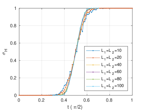
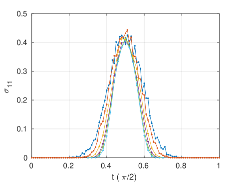
Figure 3: Disorder specific Hall conductivity $\sigma_{H}$ (left) and longitudinal conductivity $\sigma_{11}$ (right) as a function of $t$ evaluated for different sample sizes $L=10\div 100$. At $t=t_{\rm crit}=\pi/4$ the conductivity $\sigma_{11}$ saturates to a critical value $\sigma_{11}^{*}\simeq 0.4$ at large length scales, signaling Anderson de-localization at criticality. The value of $\sigma_{11}^{*}$ is close to $\simeq 0.6$ reported for the critical conductance of conventional IQHE systems, see Ref. Evers and Mirlin, 2008 for the review.

We now turn to the analysis of the second correlation function,

$$\widetilde{\sigma}_{ii}=\frac{1}{A}\left\langle{\rm tr}\left(v_{i}G^{+}v_{i}G^{-}\right)\right\rangle_{\phi}-\frac{1}{2A}{\rm tr}(v_{i}^{2}),$$ (22)

which defines the longitudinal conductivities and measures the mobility of the system. Its formal derivation, as well as the derivation of the Hall response $\widetilde{\sigma}_{H}$, see Eq. (5), is provided in Appendix A. We note here that the 2nd piece in Eq. (22) plays a role of a diamagnetic term in case of the Floquet system. Employing as above the spectral decomposition, one then finds

$$\widetilde{\sigma}_{ii}=\frac{1}{A}\sum_{m,n}\frac{|\langle m|v_{i}|n\rangle|^{2}}{1-e^{i(\epsilon_{n}-\epsilon_{m})^{+}}}-\frac{1}{2A}\sum_{m,n}|\langle m|v_{i}|n\rangle|^{2}.$$ (23)

At this point we can use once again the relation (19). Noting that $\sum_{\pm}({1-e^{\pm i\omega}})^{-1}=1$, one sees that off-diagonal terms with $n\neq m$ are canceled out in Eq. (23). We then regularize $\delta(0)=A/2\pi$ to arrive at

$$\widetilde{\sigma}_{ii}=\frac{1}{2\pi}\sum_{m}|\langle m|v_{i}|m\rangle|^{2}.$$ (24)

Results (20), (21) and (24) will serve as a basis for our numerical analysis discussed in Sec. IV.3 below.

IV.3 Numerical test

In this section, we put the results for longitudinal and Hall conductivities analytically obtained above to a numerical test. Our numerical simulations for the disorder specific observables are shown in Fig. 3. In these plots each $t$ corresponds to a single disorder realization which varies with $t$. We employ an enlarged unit cells of size $\rm L_{1}\times L_{2}$ with twisted boundary conditions to compute the transport coefficients using velocity–velocity response function. For further numerical details, see Appendix D. One observes that mesoscopic fluctuations which are visible at small system sizes ($A=10\times 10$) are essentially dying out for larger sizes ($A=10^{2}\times 10^{2}$) where the system becomes self-averaging. In the limit $L\to\infty$ the Hall conductivity, $\sigma_{H}$, tends to the step function $\theta(t-t_{\rm crit})$, see Fig. 3 (left). At the same time the longitudinal conductivity, $\sigma_{11}$, tends to zero with $L\to\infty$ whenever $t\neq t_{\rm crit}$. On the other hand, at $t=t_{\rm crit}$ the system flows to IQH critical point with $\sigma_{11}={\cal O}(1)$, see Fig. 3 (right). To complement this statement, in Fig. 4 we show the spreading of the wave packet which is initially localized at the origin. In more concrete terms the disorder averaged probability

$$P(n,{\bf x}) = \sum_{\mu,\nu\in\{A,B\}}\langle|G_{\mu\nu}^{+}(n,{\bf x},{\bf 0})|^{2}\rangle_{\phi}$$ (25)

$$\equiv \sum_{\mu,\nu\in\{A,B\}}\langle|\langle\mu,{\bf x}|U^{n}_{\rm d}|\nu,{\bf 0}\rangle|^{2}\rangle_{\phi}$$

is shown after $n\gg 1$ steps in time. At criticality, $t=t_{\rm crit}$, the wave packet is clearly delocalized. In turn, its degree of localization is increased as one moves further away from the critical point.

Transport properties of two- and multi-terminal AFAI setups have been also analyzed numerically recently in Ref. Rodríguez-Mena and Foa Torres, 2019.

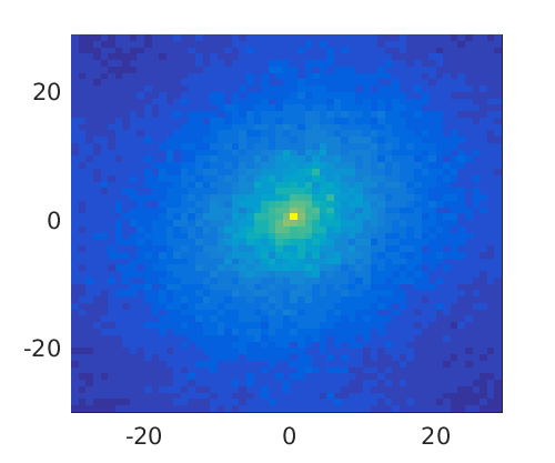
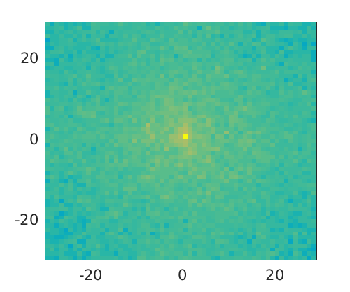
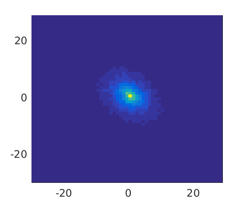
Figure 4: Disorder averaged probability distribution $P(n,{\bf x})$ (see exact definition in the main text) of a wave packet to spread on a $60\times 60$ grid after $n=600$ time steps and different values of parameter $t=\pi/5<t_{\rm crit}$ (left), $\pi/4=t_{\rm crit}$ (middle) and $7\pi/20>t_{\rm crit}$ (right). The probability distribution is averaged over $100$ disorder realizations, and normalized by the value at $\bf x=(0,0)$.

V Field theory of the AFAI

In this section, we derive the field theory discussed in the main text from first principles. This derivation has been included to make the text self contained and can be skipped by readers not interested in its technical details.

Correlation functions built as products of matrix elements of the resolvent operators (4) can be conveniently obtained from the unit-normalized Gaussian integral representation

$$1=\mathcal{Z} =\int D\psi\,\left\langle e^{-\bar{\psi}\hat{G}^{-1}\psi}\right\rangle.$$ (26)

Here, $\hat{G}=\mathrm{diag}(G^{+},G^{-})$ is a block diagonal operator containing the retarded and advanced Green function on its diagonals, and $\psi=\{\psi_{\mathbf{x}}^{sa}\}$ is a vector of Grassmann valued integration variables. The explicit representation of the exponent thus reads

$$\bar{\psi}_{\mathbf{x}}^{+a}\left(\delta_{\mathbf{x},\mathbf{y}}-e^{i\phi_{\mathbf{x}}}U_{\mathbf{x}\mathbf{y}}\right)\psi_{\mathbf{y}}^{+a}+\bar{\psi}_{\mathbf{x}}^{-a}\left(\delta_{\mathbf{x},\mathbf{y}}-U^{\dagger}_{\mathbf{x}\mathbf{y}}e^{-i\phi_{\mathbf{y}}}\right)\psi_{\mathbf{y}}^{-a},$$ (27)

where $\exp(i\phi_{\mathbf{x}})$ are the uniformly distributed phases introducing disorder and $U$ is the clean Floquet operator. Referring to Appendix A for details, Green function matrix elements are obtained from $\mathcal{Z}$ via the introduction of suitable source terms. However, for the time being, we suppress the presence of these and focus on the unit normalized ‘partition sum’, $\mathcal{Z}$.

V.1 Color-flavor transformation

The key to the derivation of an effective disorder averaged theory lies in an integral identity known as the color-flavor transform (cft) Zirnbauer (1996). This identity trades the integration over rapidly fluctuating phases, $\phi_{\mathbf{x}}$, for the integration over a composite field $Z_{\mathbf{x}}$, and in this way represents a unitary equivalent of the Hubbard-Stratonovich transformation for hermitian operators. The general cft identity reads

$$\langle\exp(\bar{\psi}^{+a}_{\mathbf{x}}e^{i\phi_{\mathbf{x}}}\varphi^{+a}_{\mathbf{x}}+\bar{\varphi}^{-a}_{\mathbf{x}}e^{-i\phi_{\mathbf{x}}}\psi^{-a}_{\mathbf{x}})\rangle_{\phi}=$$ (28)

$$\qquad=\langle\exp(\bar{\psi}^{+a}_{\mathbf{x}}Z_{\mathbf{x}}^{ab}\psi^{-b}_{\mathbf{x}}-\bar{\varphi}^{-a}_{\mathbf{x}}Z_{\mathbf{x}}^{\dagger ab}\varphi^{+b}_{\mathbf{x}})\rangle_{Z}.$$ (29)

Here, $\langle\dots\rangle_{\phi}$ is the average over uniformly distributed phases, $\prod_{\mathbf{x}}\frac{1}{2\pi}\int d\phi_{\mathbf{x}}$ with $\mathbf{x}=(\mu,x_{1},x_{2})$ combining cite and sublattice indices. On the r.h.s., $Z_{\mathbf{x}}=\{Z_{\mathbf{x}}^{a,b}\}$ are complex $R\times R$ matrices, and the functional average is defined as $\langle\dots\rangle_{Z}=\prod_{\mathbf{x}}\int dZ_{\mathbf{x}}\,\det(1+Z_{\mathbf{x}}Z_{\mathbf{x}}^{\dagger})^{-1}$. (In this expression for the measure, the replica limit $R\to 0$ has already been taken. This simplifies the notation and does not affect any results.) The integral transform (28) is exact and holds for arbitrary Grassmann vectors $\{\psi_{\mathbf{x}}\}$ and $\{\varphi_{\mathbf{x}}\}$.

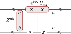
Figure 5: The idea of the color–flavor transformation: individual retarded, $\psi^{+}$, (top) and advanced, $\psi^{-}$, (bottom) wave function amplitudes fluctuate rapidly due to phase fluctuations. The composite degree of freedom $Z$ pairs these amplitudes to slowly fluctuating bilinears $\bar{\psi}^{+}\psi^{-}$.

The conceptual meaning of the cft is illustrated in Fig. 5 for the choice $\varphi_{\mathbf{x}}=U_{\mathbf{x}\mathbf{y}}\psi_{\mathbf{y}}$ relevant for our application: due to the presence of the random phases $e^{i\phi_{\mathbf{x}}}$, the bilinears $\bar{\psi}^{a}_{\mathbf{x}}e^{i\phi_{\mathbf{x}}}U_{\mathbf{x}\mathbf{y}}\psi^{a}_{\mathbf{y}}$ are rapidly fluctuating functions of the ‘color index’ $\mathbf{x}$ carrying a conserved ‘flavor’ singlet index $a$. The transformation trades them for bilinears $\bar{\psi}^{+a}_{\mathbf{x}}Z_{\mathbf{x}}^{ab}\psi^{-b}_{\mathbf{x}}$ and $(\bar{\psi}^{-b}U^{\dagger})_{\mathbf{x}}Z_{\mathbf{x}}^{\dagger ba}(U\psi^{+a})_{\mathbf{x}}$, which now carry a ‘flavor’ structure in the replica indices but, for slowly varying $Z$ no longer fluctuate rapidly in the indices $\mathbf{y}$. (The cft is called ‘color-flavor-transformation’ alluding to a similar setting in QCD, where the role of the fields $\psi$ is taken by quarks, that of $U$ by strong color-interactions, and that of $Z$ by the color-neutral yet flavored slow meson fields.)

Applied to the action (27), the cft leads to the representation

$$\mathcal{Z} =\left\langle e^{\bar{\psi}^{+}(\mathds{1}-Z)\psi^{-}+\bar{\psi}^{+}(\mathds{1}+U^{\dagger}Z^{\dagger}U)\psi^{-})}\right\rangle=$$ (30)

$$=\int DZ\,e^{-\mathrm{tr}\ln(1+ZZ^{\dagger})+\mathrm{tr}\ln(1+ZU^{\dagger}Z^{\dagger}U)}.$$ (31)

Here, the flavor indices are implicit, and the presence of the convergence generator $e^{-\delta}$ is suppressed. In the second line, we have performed the Gaussian integral over $\psi$ and elevated the determinantal measure term to become part of the action. The action now makes the tendency to slow fluctuations in the $Z$-fields explicit: spatially homogeneous configurations $Z_{\mathbf{x}}=\mathrm{const.}$ commute with $U$ and make the two terms in the action cancel. This shows that the functional integral will be dominated by slowly fluctuating configurations and is tailored to a gradient expansion.

Before turning to this expansion, we introduce the degrees of freedom $Q=T\tau_{3}T^{-1}$ central to the discussion in section III. Defining

$$T\equiv\left(\begin{matrix}\mathds{1}&Z\cr-Z^{\dagger}&\mathds{1}\end{matrix}\right),$$ (32)

the matrices $Z$ acquire a status as linear coordinates of the nonlinear manifold of $Q$-matrices. Specifically, for $R=1$, where $Q$ defines a two-sphere, and $Z\equiv z$ is just a complex number, an explicit computation of the unit vector $\mathbf{n}(z,\bar{z})$ in $Q=\tau_{i}n_{i}$ shows that $z$ is the coordinate of a stereographic projection, or Riemann sphere representation. For general $R$, the matrices $Z$ define linear coordinates of the symmetric space $\mathrm{U}(2R)/\mathrm{U}(R)\times\mathrm{U}(R)$ such that $Z=0$ represents the ‘north pole’, $Q=\tau_{3}$, and $Z\to\infty$ the ‘south pole’, $\theta=-\tau_{3}$.

A straightforward manipulation of block matrices brings the above representation of the action into the form

$$S=-\frac{1}{2}\sum_{s=\pm}\mathrm{tr}\ln\left(1+X_{s}P^{s}\right),$$ (33)

$$X_{+}\equiv T^{-1}U^{\dagger}[T,U],\quad X_{-}\equiv T^{-1}U[T,U^{\dagger}],$$

where $P^{\pm}=\{\delta^{s,\pm}\delta^{s^{\prime},\pm}\}$ are projectors onto the retarded or advanced index sector. In this form, the action is tailored for a gradient expansion. The reason is that the commutators individually vanish for constant $T$. This means that in a continuum theory an expansion up to $n$th order in these will contain at least $n$ derivatives. For our purposes an expansion to second order is sufficient,

$$S=S^{(1)}+S^{(2)},$$ (34)

$$S^{(1)}=-\frac{1}{2}\sum_{s}\mathrm{tr}(X_{s}P^{s}),\quad S^{(2)}=\frac{1}{4}\sum_{s}\mathrm{tr}((X_{s}P^{s})^{2}).$$

The continuum representation of these expressions is most economically formulated in the language of Wigner transforms. Temporarily using carets to distinguish operators $\hat{X}(\mathbf{x}_{1},\mathbf{x}_{2})$ from functions, we define

$$X(\mathbf{x},\mathbf{k})=\int d^{d}x\,e^{i\mathbf{k}\cdot\Delta\mathbf{x}}\hat{X}(\mathbf{x}+\frac{1}{2}\Delta\mathbf{x},\mathbf{x}-\frac{1}{2}\Delta\mathbf{x}).$$

Transformed in this way, the real-space operators $\hat{T}(\mathbf{x})\to T(\mathbf{x})$ become functions of $\mathbf{x}$ and the momentum-space $\hat{U}(\mathbf{k})\to U(\mathbf{k})$ functions of the conjugate momentum, $\mathbf{k}$. In Wigner language, matrix products are evaluated as Moyal products, $(\hat{X}\hat{Y})\to(X\ast Y)=Xe^{\frac{i}{2}(\partial^{\prime}_{x_{i}}\partial_{k_{i}}-\partial^{\prime}_{k_{i}}\partial_{x_{i}})}Y$, where derivatives carrying a prime act to the left and we omitted the arguments in $X(\mathbf{x},\mathbf{k})$ for brevity. Specifically, for operators diagonal in either the $\mathbf{x}$– or the $\mathbf{k}$–representation, this defines the Moyal expansions

$$T*U =TU+\frac{i}{2}\partial_{i}T\partial_{i}U+\dots,$$ (35)

$$U*T =UT-\frac{i}{2}\partial_{i}U\partial_{i}T+\dots,$$ (36)

where the derivatives $\partial_{i}$ act either on $\mathbf{x}$ or $\mathbf{k}$. Finally, note that in Moyal language traces are to be interpreted as $\mathrm{tr}(\dots)=\int d^{2}x\int d^{2}k\,\mathrm{tr}(\dots)$, where the measure $d^{2}k=dk_{1}dk_{2}/(2\pi)^{2}$, and the trace on the right extends over the internal indices of the theory.

V.2 Diffusive action

As a warm up to the somewhat more involved topological action, we consider the derivation of Eq. (8). This action is obtained from the continuum-Moyal expansion of the second order term $S^{(2)}$. At this level, it is sufficient to Moyal-expand each of the factors $X_{s}$ to first order in derivatives. Application of the rules Eq. (35) gives

$$X_{\pm}\simeq iA_{i}\Psi^{\pm}_{i},\quad A_{i}\equiv T^{-1}\partial_{i}T,$$

$$\Psi^{+}=U^{\dagger}\partial_{i}U,\quad\Psi^{-}=U\partial_{i}U^{\dagger},$$

and the substitution of this expansion into $S^{(2)}$ leads to

$$S^{(2)}=\frac{1}{4}\sum_{s}\int d^{2}k\,\mathrm{tr}(\Psi^{s}_{i}\Psi^{s}_{j})\int d^{2}x\,\mathrm{tr}(A_{i}P^{s}A_{j}P^{s}).$$

Using that $U^{\dagger}\partial_{i}U=-\partial_{i}U^{\dagger}U$, the $k$-dependent part in this expression becomes $\int d^{2}k\,\mathrm{tr}(\Psi^{+}_{i}\Psi^{+}_{j})=\int d^{2}k\,\mathrm{tr}(\Psi^{-}_{i}\Psi^{-}_{j})=\sigma_{ij}^{(0)}$, as defined in section III. Turning to the real space part, a quick calculation shows that $\sum_{s}\mathrm{tr}(A_{i}P^{s}A_{j}P^{s})=\frac{1}{4}\mathrm{tr}([A_{i},\tau_{3}][A_{j},\tau_{3}])-\mathrm{tr}(A_{i}A_{j})=\frac{1}{4}\mathrm{tr}(\partial_{i}Q\partial_{j}Q)-\mathrm{tr}(A_{i}A_{j})$. In combination with $\sigma^{(0)}_{ij}$, the first term on the r.h.s. yields Eq. (64), and the second, gives a contribution

$$-\frac{1}{2}\sigma_{ij}^{(0)}\mathrm{tr}(A_{i}A_{j}),$$ (37)

which we will see cancels against another one from the expansion of $S^{(1)}$.

V.3 Topological action

We now focus our attention on the first order term $S^{(1)}$. Naively, one might think that a term of first order in a gradient expansion might vanish by symmetry. On the other hand, this is a system with inbuilt chirality. The key to understanding who wins the argument lies in an elegant trick, first applied by Pruisken Pruisken (1984) in a slightly different manner adapted to the IQH.

We start by considering the ‘$+$’ contribution to the action $S^{(1)}$,

$$S^{(1)+} =-\frac{1}{2}\mathrm{tr}((T^{-1}U^{\dagger}TU-\mathds{1})P^{+})=$$

$$=\frac{1}{2}\int_{0}^{t}ds\,\partial_{s}\mathrm{tr}(T^{-1}U^{\dagger}TUP^{+}),$$

where we have introduced a continuous interpolation $s:[0,t]\to\mathrm{U}(2),s\mapsto U(s)$, such that $U(t)=U$, and $U(0)=\mathds{1}$. (In Pruisken’s construction, the role of $U$ is taken by the Green function of electrons in a magnetic field, and the interpolation parameter is energy running from the bottom of the band to the Fermi energy.)

Doing the derivative, and defining $\Psi^{+}_{s}\equiv U^{\dagger}\partial_{s}U$, this can be rewritten as

$$S^{(1)+} =\frac{1}{2}\int_{0}^{t}ds\,\mathrm{tr}(\left[\Psi_{s},T^{-1}\right][U^{\dagger},TU]P^{+}).$$

To derive this result we have used that in the replica limit ${\rm tr}\bigl{(}T(\mathbf{x})P^{+}T^{-1}(\mathbf{x})\bigr{)}=R\to 0$ for each $\mathbf{x}$. The presence of two commutators implies a minimum of two extra derivatives, meaning that each commutator individually can be evaluated at lowest order in the Moyal expansion. Application of (35) then gives

$$S^{(1)+} =\frac{1}{2}\int_{0}^{t}ds\,\mathrm{tr}(\partial_{i}\Psi^{+}_{s}\Psi^{+}_{j})\,\mathrm{tr}(\partial_{i}T^{-1}\partial_{j}TP^{+}).$$

To make further progress with this representation, we need a technical formula proven in Appendix C,

$${b}_{ij}\equiv\mathrm{tr}((\partial_{j}\Psi^{+}_{s})\Psi^{+}_{k})={b}_{ij}^{s}+{b}_{ij}^{a},$$ (38)

$${b}_{ij}^{s}=-\frac{1}{2}\partial_{s}\,\mathrm{tr}(\Psi^{+}_{i}\Psi_{j}^{+}),\quad{b}_{ij}^{a}=-\frac{1}{2}\epsilon_{ij}\mathrm{tr}(\Psi^{+}_{s}[\Psi^{+}_{x},\Psi^{+}_{y}]),$$

splitting the $\mathbf{k}$-part of the action into a contribution symmetric and antisymmetric in the indices $i,j$. Concerning the former, we note $\int_{0}^{s}ds\,{b}_{ij}^{s}=-\frac{1}{2}\,\mathrm{tr}(\Psi^{+}_{i}\Psi_{j}^{+})=-\frac{1}{2}\,\mathrm{tr}(\Psi^{-}_{i}\Psi_{j}^{-})=\frac{1}{2}\sigma_{ij}^{(0)}$. Using that $P^{+}+P^{-}=\mathds{1}$, the symmetric contribution to $S^{(1)}$, obtained by adding the ‘$+$’ and the ‘$-$’, part thus assumes the form $S^{(1),s}=\frac{1}{2}\sigma_{ij}^{(0)}\,\mathrm{tr}(A_{i}A_{j})$, and cancels against (37).

Turning to the antisymmetric part, we note that

$$\int_{0}^{t}ds\,\epsilon^{lm}\mathrm{tr}(\Psi^{+}_{s}\Psi^{+}_{l}\Psi^{+}_{m})=$$

$$=\frac{1}{4\pi^{2}}\int dsd^{2}k\,\mathrm{tr}(U^{\dagger}\partial_{s}U[U^{\dagger}\partial_{1}U,U^{\dagger}\partial_{2}U])=\frac{1}{\pi}\Gamma[U],$$

where $\Gamma[U]$ is the WZW functional of Eq. (11). The corresponding ‘$-$’ term gives the same contribution with an opposite sign. This means that the antisymmetric contribution assumes the form

$$S_{\mathrm{top}}=-\frac{1}{4\pi}\Gamma[U]\int d^{2}x\,\epsilon_{ij}\,\mathrm{tr}(A_{i}A_{j}\tau_{3}).$$

Finally, a quick calculation shows that $\epsilon_{ij}\,\mathrm{tr}\left(A_{i}A_{j}\tau_{3}\right)=-\frac{1}{4}\epsilon_{ij}\mathrm{tr}\left(Q\partial_{i}Q\partial_{j}Q\right)$, which leads us to Eq. (12).

V.4 Frequency action

We conclude this section with a quick derivation of Eq. (14). Retracing the steps leading to Eq. (30), we note that in the presence of a finite difference, $\omega$, $U\to Ue^{i\omega/2}$, $U^{\dagger}\to U^{\dagger}e^{i\omega/2}$, the argument in the second logarithm generalizes to $ZU^{\dagger}Z^{\dagger}U\to e^{i\omega-2\delta}ZU^{\dagger}Z^{\dagger}U\simeq ZU^{\dagger}Z^{\dagger}U+i\omega^{+}ZZ^{\dagger}$, where in the second step we assumed smallness of the decoherence parameter $\omega^{+}\equiv\omega+2i\delta$, and noted that to leading order in an expansion the non-commutativity of $Z,Z^{\dagger}$ with $U$ may be neglected in this term. The first order expansion of the action in $\omega^{+}$ then yields, $S=S_{0}+i\omega^{+}\,\mathrm{tr}(1+ZZ^{\dagger})^{-1}ZZ^{\dagger})$. With Eq. (32) and $Q=T\tau_{3}T^{-1}$, a straightforward calculation shows the equivalence to Eq. (14).

VI Summary and discussion

In this paper, we have presented an analytical theory of topological quantum criticality in the AFAI. We have seen that the structure of this theory is essentially determined by symmetries and geometric constraints involving both the clean part of the Floquet operator, and an effective real space field describing phase coherent transport in the presence of disorder. On the same grounds, we have reasoned that the finite size AFAI does not admit the definition of an integer invariant, and that topological quantization is an emergent feature in the thermodynamic limit. The flow towards a configuration with integer quantized transverse response is equivalent to that in the static quantum Hall insulator. Formally, this connection follows from the equivalence of the effective theory of the AFAI to the Pruisken theory of the IQH. Physically, it reflects the stabilization of edge transport via bulk localization. The distinct topological phases, $\sigma=0,1$, are separated by a quantum phase transition which, likewise, is in the IQH universality class. A not entirely obvious conclusion from this equivalence is that extended Landau level center states connecting opposite surfaces of the system — present in the IQH, but absent in the present system — are not essential to IQH universality. The results discussed in this paper were obtained for an implementation of the AFAI via a specific five step driving protocol. One may ask how robust they are, e.g. to changes in the disorder distribution and/or changes in the choreography of the driving protocol. While the very nature of the question excludes a rigorous answer, it all boils down to the robustness of the AFAI quantum Hall phase itself: how violent does a perturbation imposed on an edge mode supporting topological thermodynamics phase have to be to destruct that mode? Since the phase is stabilized by two robust principles, $2d$ Anderson localization, and the oriented hopping dynamics of the clean system, we believe in a high level of protection. Within the framework of the field theoretical construction this reflects in the well known robustness of, say, Wess-Zumino functionals to the presence of perturbations at the microscopic level. However, it would take a study way beyond the present one quantitatively probe the tolerance windows of the modeling.

The geometric principles underlying the present construction carry over to other FTI in other dimensions and symmetry classes. In fact, they can be extended beyond the class of topological insulators to describe a topologically protected Floquet metals. These systems have no analog in static quantum matter and will be the subject of a forthcoming publication.

Appendix A Source terms

In the following we demonstrate that the coupling of the theory to sources as in Eq. (15), (16), and (17) yields the disorder averaged linear response coefficients (5) and (22). The way to show this is to retrace the steps leading to the effective action, with the sources kept in place. Performing the source differentiation at the early steps of the construction then yields Eqs. (5) and (22).

Since $Q\to SQS^{-1}$ and $Q=T\tau_{3}T^{-1}$, the coupling of sources is equivalent to the replacement $T\to ST\equiv T_{S}$. The sourced action is thus generated by expansion of the prototype action Eq. (33) evaluated on $T_{S}$. From here, one may go back to the original $\psi$-representation in a sequence of operations that is straightforward yet somewhat tedious:

We first note that the same block matrix operations that led from Eq. (30) to Eq. (33) show that the two terms $s=\pm$ in the latter are identical. In the present section, we find it convenient to work with the ‘$-$’ variant, so that the sourced action reads

$$S[T_{S}] =-\mathrm{tr}\ln(1+T_{S}^{-1}(UT_{S}U^{\dagger}-T_{S})P^{-})=\mathrm{tr}\ln(T)-\mathrm{tr}\ln(T+(UTU^{\dagger}-T+(S^{-1}S^{U})UTU^{\dagger})P^{-}),$$

where, up to the required second order in the source parameters $q_{i}$ of Eq. (15),

$$S^{-1}S^{U}\equiv S^{-1}(USU^{\dagger}-S)=P^{(1)}\left(\begin{matrix}w&z\cr\bar{z}&\bar{w}\end{matrix}\right),$$

where

$$w\equiv-i\epsilon^{ij}q_{i}q^{U}_{j}-q_{i}q^{U}_{i}+\tfrac{1}{2}\left(Uq_{i}^{2}U^{\dagger}-q_{i}^{2}\right),\qquad z=q^{U}_{1}-iq^{U}_{2}.$$ (39)

With the help of Eq. (32), the action can then be written as

$$S=\mathrm{tr}\ln(T)-\mathrm{tr}\ln\left(\begin{matrix}1&UZU^{\dagger}+P^{(1)}(wUZU^{\dagger}+z)\cr-Z^{\dagger}&1+P^{(1)}(\bar{z}UZU^{\dagger}+\bar{w})\end{matrix}\right).$$

We proceed by representing the second determinant as a Gaussian integral and un-doing the cft. On the 1st step of this procedure the fermion action is of the form

$$S_{{\rm I}}=\mathrm{tr}\ln(T)+\bar{\psi}^{+}\psi^{+}+(\bar{\psi}^{+}(1+P^{(1)}w)+\bar{\psi}^{-}P^{(1)}\bar{z})UZU^{\dagger}\psi^{-}+\bar{\psi}^{+}P^{(1)}z\psi^{-}-\bar{\psi}^{-}Z^{\dagger}\psi^{+}+\bar{\psi}^{-}(1+P^{(1)}\bar{w})\psi^{-}.$$ (40)

On introducing auxiliary spinors

$$\qquad\phi^{-}=U^{\dagger}\psi^{-},\qquad\bar{\phi}^{+}=\left(\bar{\psi}^{+}(1+P^{(1)}w)+\bar{\psi}^{-}P^{(1)}\bar{z}\right)U,\qquad$$ (41)

this action becomes

$$S_{{\rm I}}=\mathrm{tr}\ln(T)+\bar{\psi}^{+}\psi^{-}+\bar{\psi}^{+}P^{(1)}z\psi^{-}+\bar{\psi}^{-}(1+P^{(1)}\bar{w})\psi^{-}+\bar{\phi}^{+}Z\phi^{-}-\bar{\psi}^{-}Z^{\dagger}\psi^{+},$$ (42)

and its $Z$-dependent part can be further subjected to cft, see Eq. (28). In this way we arrive at

$$S_{{\rm II}}=S_{0}-\bar{\psi}^{+1}wU_{\rm d}\psi^{+1}+\bar{\psi}^{-1}\bar{w}\psi^{-1}+\bar{\psi}^{+1}z\psi^{-1}-\bar{\psi}^{-1}\bar{z}U_{\rm d}\psi^{+1},$$ (43)

where $S_{0}$ is the source-free action, and the numerical superscript in $\psi^{\sigma,1}$ refers to the replica index. At this point, the differentiation in the source parameters $a_{i}$ sitting in $w$ and $z$ — they are expressed in terms of $q_{i}\equiv a_{i}x_{i}$ and $q^{U}_{i}\equiv a_{i}v_{i}$, — can be carried out. For the Hall conductivity this leads to

$$\widetilde{\sigma}_{H} =\frac{1}{2iA}\left.\frac{\partial^{2}}{\partial a_{1}\partial a_{2}}\right|_{a=0}\mathcal{Z}(a)$$ (44)

$$=\frac{1}{2iA}\left\langle-i\bar{\psi}^{+1}\epsilon^{ij}x_{i}v_{j}U_{\rm d}\psi^{+1}-i\bar{\psi}^{-1}\epsilon^{ij}x_{i}v_{j}\psi^{-1}-i\bar{\psi}^{+1}v_{1}\psi^{-1}\bar{\psi}^{-1}v_{2}U_{\rm d}\psi^{+1}+i\bar{\psi}^{+1}v_{2}\psi^{-1}\bar{\psi}^{-1}v_{1}U_{\rm d}\psi^{+1}\right\rangle$$ (45)

$$=\frac{1}{2A}\Bigl{(}\epsilon^{ij}\mathrm{tr}(x_{i}v_{j})+\mathrm{tr}(v_{1}G^{-}v_{2}G^{+}-v_{2}G^{-}v_{1}G^{+})\Bigr{)},$$ (46)

where in the last step we used that $\langle G^{-}\rangle=1$ and $\langle G^{+}U_{\rm d}\rangle=0$ due to the random fluctuations of $U_{\rm d}$, while $\epsilon^{ij}\langle v_{i}G^{-}v_{j}U_{\rm d}G^{+}\rangle=\epsilon^{ij}\langle v_{i}G^{-}v_{j}G^{+}\rangle$. The latter can be seen by representing $U_{\rm d}=1-(G^{+})^{-1}$ in the limit $\delta\to 0^{+}$. The final result (44) contains the two terms entering the correlation function (5). Similarly, for the longitudinal conductivity one derives

$$\widetilde{\sigma}_{11} =\frac{1}{2A}\left.\frac{\partial^{2}}{\partial a_{1}^{2}}\right|_{a=0}\mathcal{Z}(a)$$ (47)

$$=\frac{1}{A}\left\langle-\bar{\psi}^{+1}x_{1}v_{1}U_{\rm d}\psi^{+1}+\tfrac{1}{2}\bar{\psi}^{+1}[U_{\rm d},x_{1}^{2}]\psi^{+1}+\bar{\psi}^{-1}x_{1}v_{1}\psi^{-1}-\tfrac{1}{2}\bar{\psi}^{-1}(U_{\rm d}x_{1}^{2}U_{\rm d}^{\dagger}-x_{1}^{2})\psi^{-1}-\bar{\psi}^{+1}v_{1}\psi^{-1}\bar{\psi}^{-1}v_{1}U_{\rm d}\psi^{+1}\right\rangle$$ (48)

$$=\frac{1}{A}\Bigl{(}-\mathrm{tr}(x_{1}v_{1})+\mathrm{tr}(v_{1}G^{-}v_{1}U_{\rm d}G^{+})\Bigl{)}=\frac{1}{A}\Bigl{(}-\frac{1}{2}\mathrm{tr}(v_{1}^{2})+\mathrm{tr}(v_{1}G^{-}v_{1}G^{+})\Bigl{)}.$$ (49)

To get the very last result above we have once again employed $U_{\rm d}=1-(G^{+})^{-1}$ and used the relation $-\mathrm{tr}(x_{1}v_{1})=\tfrac{1}{2}\mathrm{tr}(v_{1}^{2})$. In its final form the result (47) equals to the correlation function (22). To summarize, the above calculations establish the equality $\widetilde{\sigma}_{H}=\sigma_{H}(L)$ and $\widetilde{\sigma}_{11}=\sigma_{11}(L)$ of the running coupling constants of the field theory at scale $L$ and the microscopically defined response functions.

Appendix B Proof of the equivalence $\sigma^{\rm II}=\sigma_{H}^{(0)}$

The proof of this equivalence is very similar to the derivation of the topological action in Sec. V.3. On introducing the interpolation $U(s)$ as it was done before and using $\Psi_{s}^{-}\equiv U\partial_{s}U^{\dagger}$ one has

$$\sigma^{\rm II} = \frac{\epsilon_{ij}}{2A}\int_{0}^{{t}}d{s}\,\partial_{s}{\rm tr}(x_{i}Ux_{j}U^{\dagger})$$ (50)

$$= \frac{\epsilon_{ij}}{2A}\int_{0}^{{t}}d{s}\,{\rm tr}(x_{i}Ux_{j}U^{\dagger}\Psi^{-}_{{s}}-x_{i}\Psi^{-}_{{s}}Ux_{j}U^{\dagger})$$

$$= \frac{\epsilon_{ij}}{2A}\int_{0}^{{t}}d{s}\,{\rm tr}\left([\Psi^{-}_{{s}},x_{i}]Ux_{j}U^{\dagger}\right).$$

At this stage we use the exact relations

$$Ux_{j}U^{\dagger}-x_{j}=iU\partial_{j}U^{\dagger},\qquad[\Psi_{s}^{-},x_{i}]=-i\partial_{i}\Psi^{-}_{s},$$ (51)

and an obvious identity ${\rm tr}([\Psi_{{s}}^{-},x_{i}]x_{j})\epsilon_{ij}=0$. Taking them into account by means of the following chain of transformations,

$$\sigma^{\rm II} = \frac{\epsilon_{ij}}{2A}\int_{0}^{{t}}d{s}\,{\rm tr}\left(\partial_{i}\Psi_{s}^{-}U\partial_{j}U^{\dagger}\right)$$

$${=} -\frac{\epsilon_{ij}}{8\pi^{2}}\int dsd^{2}k\,{\rm tr}\left(\Psi_{s}^{-}\partial_{i}U\partial_{j}U^{\dagger}\right)$$

$$= \frac{\epsilon_{ij}}{8\pi^{2}}\int dsd^{2}k\,{\rm tr}\left(\Psi_{s}^{-}\Psi_{i}^{-}\Psi_{j}^{-}\right)=\frac{1}{2\pi}\Gamma[U]=\sigma_{H}^{(0)},$$

one accomplishes the proof, where in the second line we have used an integration by parts in momentum space.

Appendix C Proof of Eq. (38)

To prove Eq. (38), we first note that the trace in ${b}_{ij}\equiv\mathrm{tr}((\partial_{j}\Psi^{+}_{s})\Psi^{+}_{k})=\mathrm{tr}(\partial_{j}(U^{\dagger}\partial_{s}U)U^{\dagger}\partial_{k}U)$ implies an integration over momenta, $\mathbf{k}$, with periodic boundary conditions. We may thus rearrange momenta via integrations by parts. Applying this freedom to the $j$-derivative, we obtain

$${b}_{ij} =\frac{1}{2}\mathrm{tr}(\partial_{i}(U^{\dagger}\partial_{s}U)(U^{\dagger}\partial_{j}U-\partial_{j}U^{\dagger}U))=$$

$$=-\frac{1}{2}\mathrm{tr}(U^{\dagger}\partial_{s}U(\partial_{i}U^{\dagger}\partial_{j}U-\partial_{j}U^{\dagger}\partial_{i}U+$$

$$\hskip 56.9055pt+U^{\dagger}\partial^{2}_{ij}U-\partial^{2}_{ij}U^{\dagger}U))=$$

$$=\frac{1}{2}\mathrm{tr}(\Psi_{s}^{+}[\Psi_{i}^{+},\Psi_{j}^{+}]+\partial_{s}U^{\dagger}\partial^{2}_{ij}U+\partial_{s}U\partial^{2}_{ij}U^{\dagger}).$$

The first term in this expression defines the anti-symmetric contribution to Eq. (38). A double partial integration in $k_{i,j}$ brings the second into the form, $\frac{1}{2}\partial_{s}\,\mathrm{tr}(U^{\dagger}\partial^{2}_{ij}U)=-\frac{1}{2}\partial_{s}\,\mathrm{tr}(\Psi^{+}_{i}\Psi_{j}^{+})$, which is the symmetric contribution.

Appendix D Numerical details

To compute the Hall, $\widetilde{\sigma}_{H}$, and longitudinal, $\widetilde{\sigma}_{11}$, conductivities for a specific disorder realization in Fig. 3, we have used an enlarged unit cell of lattice size $\rm L_{1}\times L_{2}$ with a twisted boundary condition across the unit cell boundary by adding phase $\theta_{1,2}$ in the hopping amplitudes:

$$U^{\mathbb{\theta}}_{\mathbf{x}\mathbf{y}} = U_{\mathbf{x}\mathbf{y}}e^{i\theta_{1}\delta_{x_{1}-y_{1},\rm L_{1}-1}+i\theta_{2}\delta_{x_{2}-y_{2},\rm L_{2}-1}}$$ (52)

$$\times e^{-i\theta_{1}\delta_{x_{1}-y_{1},-\rm L_{1}+1}-i\theta_{2}\delta_{x_{2}-y_{2},-\rm L_{2}+1}},$$

where $\mathbf{x}=(x_{1},x_{2})$, $\mathbf{y}=(y_{1},y_{2})$, and $U_{\mathbf{x}\mathbf{y}}$ is a matrix element of the clean Floquet operator in real space. Notice that our model contains nearest neighbor hopping only. The velocity operators are then computed through $v_{i}=U^{\mathbb{\theta}\dagger}\partial_{\theta_{i}}U^{\mathbb{\theta}}$, which in fact is independent both of $\theta_{1,2}$ and disorder. By taking a set of eigenvalues and eigenvectors of $U^{\mathbb{\theta}}$, $\sigma^{I}$ in (20) and $\widetilde{\sigma}_{ii}$ in (24) are computed for a specific twisted boundary $(\theta_{1},\theta_{2})$. Lastly, the conductivities are averaged over $\theta_{1,2}\in[0,2\pi]$.

Appendix E Hall conductivity

In this appendix we derive equivalent representation for the Hall response coefficient, $\tilde{\sigma}_{H}=\sigma^{\rm I}+\sigma^{\rm II}$, which in the localized regime will enable us to relate $\tilde{\sigma}_{H}$ to the number of topological chiral edge modes. We start from Eqs. (20) and (21) and transform $\sigma^{\rm II}$ in a different way as compared to Appendix B. To this end, consider a cylindrical geometry of a width $L_{1}$ and a circumference $L_{2}$ implying periodic boundary conditions along $x_{2}$-direction. A cylinder has two boundaries where delocalized chiral edge states may propagate. In addition to the velocity operator $v_{2}=Ux_{2}U^{\dagger}-x_{2}$ we introduce another one,$\bar{v}_{2}=-U^{\dagger}x_{2}U+x_{2}$. With the help of the latter

$${\rm tr}(v_{1}x_{2}) = {\rm tr}(Ux_{1}U^{\dagger}-x_{1})x_{2}$$

$$= {\rm tr}\,x_{1}(U^{\dagger}x_{2}U-x_{2})=-{\rm tr}(x_{1}\bar{v}_{2}),$$

and therefore

$$\sigma_{12}^{\rm II}=\frac{1}{2}{\rm tr}\,x_{1}(v_{2}+\bar{v}_{2}).$$ (54)

To proceed, we first analyze the off-diagonal terms of $\sigma_{12}^{\rm II}$ in the eigenbasis of $U$. Denoting the off-diagonal contribution as $\widetilde{\sigma}_{12}^{\rm II}$, one can write for the matrix elements of velocity operators $v_{2}$ (below $m\neq n$),

$$\langle n|v_{2}|m\rangle = \langle n|x_{2}|m\rangle(e^{i(\epsilon_{m}-\epsilon_{n})}-1),$$ (55)

$$\langle n|\bar{v}_{2}|m\rangle = \langle n|x_{2}|m\rangle(1-e^{-i(\epsilon_{m}-\epsilon_{n})}),$$ (56)

which yields a nice cancellation,

$$\widetilde{\sigma}_{12}^{\rm II} = \frac{i}{A}\sum_{m\neq n}\langle m|x_{1}|n\rangle\langle n|x_{2}|m\rangle\sin(\epsilon_{m}-\epsilon_{n})$$

$$= \frac{i}{2A}\sum_{m\neq n}\langle m|v_{1}|n\rangle\langle n|v_{2}|m\rangle\cot\left(\frac{\epsilon_{m}-\epsilon_{n}}{2}\right)=-\sigma_{12}^{\rm I},$$

where in the last line Eq. (20) was used. Hence, only diagonal terms contribute to the final result and

$$\widetilde{\sigma}_{H}=\frac{1}{2A}\sum_{m}\langle m|x_{1}|m\rangle\langle m|v_{2}+\bar{v}_{2}|m\rangle.$$ (58)

At this point, a subtlety comes into play — the diagonal matrix elements of velocity operators $v_{2}$ and $\bar{v}_{2}$ can be only defined without a reference to the position operator $x_{2}$. In the clean limit and infinite circumference, $L_{2}\to\infty$, one can set $x_{2}=i\partial_{k_{2}}$ (where $k_{2}\in[-\pi,\pi]$ is the Bloch momentum) so that

$$\langle m|v_{2}|m\rangle = \langle m|U(i\partial_{k_{2}}U^{\dagger})|m\rangle,$$

$$\langle m|\bar{v}_{2}|m\rangle = -\langle m|U^{\dagger}(i\partial_{k_{2}}U)|m\rangle.$$ (59)

Provided the system is homogeneous in $x_{2}$-direction, the momentum $k_{2}$ is conserved and the eigenstate has the form $|m\rangle\equiv|l,k_{y}\rangle$, where $l$ is a discrete quantum number stemming from the quantization along $x_{1}$-direction. For this configuration we find

$$\widetilde{\sigma}_{H}=\frac{1}{L_{1}}\sum_{l}\int_{0}^{2\pi}\frac{dk_{2}}{2\pi}\langle l,k_{2}|x_{1}|l,k_{2}\rangle\frac{\partial\epsilon_{l}(k_{2})}{\partial k_{2}}.$$ (60)

The above result can be now extended to the general situation when $L_{2}$ is finite and the periodically driven Floquet system includes spatial disorder. In this case there is no continuous momentum variable $k_{2}$ to differentiate. However, one can define the Floquet operator $\hat{U}(\theta_{2})$ for a system with twisted boundary conditions in $x_{2}$-direction which has a flux-dependent spectrum of quasi-energies $\epsilon_{m}(\theta_{2})$, see Appendix D. In physical terms it corresponds to the flux $\theta_{2}$ of a magnetic field threading a cylinder along the axis $x_{1}$. Then the above result (60) should be generalized as

$$\widetilde{\sigma}_{H}=\frac{1}{L_{1}}\sum_{m}\int_{0}^{2\pi}\frac{d\theta_{2}}{2\pi}\langle m,\theta_{2}|x_{1}|m,\theta_{2}\rangle\frac{\partial\epsilon_{m}(\theta_{2})}{\partial\theta_{2}}.$$ (61)

To justify this expression, we refer to a well known trick: one considers an auxiliary periodic in $x_{2}$-direction Floquet system composed of infinite number of supercells of length $L_{2}$ sharing the same realization of disorder, and then appeals to the previous Eq. (60).

The relation (61) has a transparent meaning in the localized phase where, as we show below, it equals to the number of chiral edge modes, $n_{\rm edge}$. Indeed, the states localized in the bulk are not sensitive to a variation of $\theta_{2}$ (for them $\partial\epsilon_{m}(\theta_{2})/\partial\theta_{2}\to 0$) and thus do not contribute to (61). On other hand, for the set of right/left boundary states, which we denote as $|b^{\pm},\theta_{2}\rangle$ where $0\leq b^{\pm}<{\cal N}$, the matrix elements $\langle b^{\pm},\theta_{2}|x_{1}|b^{\pm},\theta_{2}\rangle\to\pm L_{1}/2$ and group velocities are non-zero, $\partial\epsilon_{b}^{\pm}(\theta_{2})/\partial\theta_{2}\gtrless 0$. Importantly, these states are subjected to the spectral flow, i.e.

$$\epsilon_{b}^{\pm}(\pi-0)\to\epsilon_{b+1}^{\pm}(-\pi+0),\quad b=0,\dots,\,{\cal N}-1.$$ (62)

and thereby form either a single or a number of chiral edge modes, cf. Fig. 3 in Ref. Titum et al., 2016. Note that the number of chiral edge states, $n_{\rm edge}$, is smaller than the number of edge states, ${\cal N}$, since few $b$’s will typically combine to create a chiral mode. Hence, for $\widetilde{\sigma}_{H}$ we find a limiting expression valid in the Anderson localized phase,

$$\widetilde{\sigma}_{H}\to\frac{1}{2}\sum_{b=0}^{{\cal N}-1}\int_{0}^{2\pi}\frac{d\theta_{2}}{2\pi}\left(\frac{\partial\epsilon_{b}^{+}(\theta_{2})}{\partial\theta_{2}}-\frac{\partial\epsilon_{b}^{-}(\theta_{2})}{\partial\theta_{2}}\right).$$ (63)

Because of the spectral flow (62), the above relation shows how many times the quasi-energy spectrum winds around a cirlce (the full Bloch zone) $[-\pi,\pi]$ as the flux $\theta_{2}$ varies from 0 to $2\pi$ and in this way $\widetilde{\sigma}_{H}$ counts the number of chiral states $n_{\rm edge}$. The analysis in this Appendix is in line with the previous work by Titum et al.Titum et al. (2016), see in particular their discussion in section III.B.

References

- Oka and Aoki (2009) Takashi Oka and Hideo Aoki, “Photovoltaic Hall effect in graphene,” Phys. Rev. B 79, 081406 (2009).
- Lindner and Refael (2011) Netanel H. Lindner and Victor Refael, Giland Galitski, “Floquet topological insulator in semiconductor quantum wells,” Nature Physics 7, 490–495 (2011).
- Kitagawa et al. (2012) Takuya Kitagawa, Matthew A. Broome, Alessandro Fedrizzi, Mark S. Rudner, Erez Berg, Ivan Kassal, Alán Aspuru-Guzik, Eugene Demler, and Andrew G. White, “Observation of topologically protected bound states in photonic quantum walks,” Nature Communications 3, 882 EP – (2012), article.
- Edge and Asboth (2015) Jonathan M. Edge and Janos K. Asboth, “Localization, delocalization, and topological transitions in disordered two-dimensional quantum walks,” Phys. Rev. B 91, 104202 (2015).
- Dahlhaus et al. (2011) J. P. Dahlhaus, J. M. Edge, J. Tworzydło, and C. W. J. Beenakker, “Quantum Hall effect in a one-dimensional dynamical system,” Phys. Rev. B 84, 115133 (2011).
- Tian et al. (2016) Chushun Tian, Yu Chen, and Jiao Wang, “Emergence of integer quantum Hall effect from chaos,” Phys. Rev. B 93, 075403 (2016).
- Titum et al. (2016) Paraj Titum, Erez Berg, Mark S. Rudner, Gil Refael, and Netanel H. Lindner, “Anomalous Floquet-Anderson Insulator as a Nonadiabatic Quantized Charge Pump,” Phys. Rev. X 6, 021013 (2016).
- Jiang et al. (2011) Liang Jiang, Takuya Kitagawa, Jason Alicea, A. R. Akhmerov, David Pekker, Gil Refael, J. Ignacio Cirac, Eugene Demler, Mikhail D. Lukin, and Peter Zoller, “Majorana fermions in equilibrium and in driven cold-atom quantum wires,” Phys. Rev. Lett. 106, 220402 (2011).
- Rechtsman et al. (2013) Mikael C. Rechtsman, Julia M. Zeuner, Yonatan Plotnik, Yaakov Lumer, Daniel Podolsky, Felix Dreisow, Stefan Nolte, Mordechai Segev, and Alexander Szameit, “Photonic floquet topological insulators,” Nature 496, 196–200 (2013).
- Potirniche et al. (2017) I.-D. Potirniche, A. C. Potter, M. Schleier-Smith, A. Vishwanath, and N. Y. Yao, “Floquet symmetry-protected topological phases in cold-atom systems,” Phys. Rev. Lett. 119, 123601 (2017).
- Higashikawa et al. (2019) Sho Higashikawa, Masaya Nakagawa, and Masahito Ueda, “Floquet chiral magnetic effect,” Phys. Rev. Lett. 123, 066403 (2019).
- Kitagawa et al. (2010) Takuya Kitagawa, Erez Berg, Mark Rudner, and Eugene Demler, “Topological characterization of periodically driven quantum systems,” Phys. Rev. B 82, 235114 (2010).
- Rudner et al. (2013) Mark S. Rudner, Netanel H. Lindner, Erez Berg, and Michael Levin, “Anomalous edge states and the bulk-edge correspondence for periodically driven two-dimensional systems,” Phys. Rev. X 3, 031005 (2013).
- Roy and Harper (2017) Rahul Roy and Fenner Harper, “Periodic table for floquet topological insulators,” Phys. Rev. B 96, 155118 (2017).
- Kitaev (2009) Alexei Kitaev, “Periodic table for topological insulators and superconductors,” AIP Conference Proceedings 1134, 22–30 (2009), https://aip.scitation.org/doi/pdf/10.1063/1.3149495 .
- Zirnbauer (1996) Martin R. Zirnbauer, “Supersymmetry for systems with unitary disorder: circular ensembles,” Journal of Physics A: Mathematical and General 29, 7113 (1996).
- Altland et al. (2015) Alexander Altland, Sven Gnutzmann, Fritz Haake, and Tobias Micklitz, “A review of sigma models for quantum chaotic dynamics,” Reports on Progress in Physics 78, 086001 (2015).
- Note (1) Note that is defined w.r.t. the clean part of the Floquet operator, . Had one start from another definition, , one would see that the random part doesn’t contribute to (indeed, ) and hence one finds .
- Wegner (1979) Franz Wegner, “The mobility edge problem: Continuous symmetry and a conjecture,” Zeitschrift für Physik B: Condensed Matter 35, 207–210 (1979).
- Efetov et al. (1980) K. B. Efetov, A. I. Larkin, and D. E. Khmel’nitskii, “Interaction of diffusion modes in the theory of localization,” JETP 52, 568 (1980).
- Pruisken and Schäfer (1982) Adrianus M.M. Pruisken and Lothar Schäfer, “The Anderson model for electron localisation non-linear model, asymptotic gauge invariance,” Nuclear Physics B 200, 20 – 44 (1982).
- Efetov and Larkin (1983) K. B. Efetov and A. I. Larkin, “Kinetics of a quantum particle in long metallic wires,” Sov. Phys. JETP 58, 444–451 (1983).
- Pruisken (1984) A.M.M. Pruisken, “On localization in the theory of the quantized Hall effect: A two-dimensional realization of the theta-vacuum,” Nuclear Physics B 235, 277 – 298 (1984).
- Efetov (1997) K. B. Efetov, Sypersymmetry in Disorder and Chaos (Cambridge University Press, Cambridge, 1997).
-
Note (2)
For completeness, we mention that the microscopic derivation
below leads to the more general expression
where plays a role of the symmetric part of the conductivity tensor , . In the present system, without external magnetic field, we do not have an Onsager reciprocity relation () and the symmetric contribution to the conductivity tensor may have a skew contribution. However, the bare coupling of this contribution is small and it vanishes at first order in perturbation theory due to the spatial asymmetry of . We therefore ignore this contribution throughout.(64) - Altland and Simons (2010) Alexander Altland and Ben Simons, Condensed Matter Theory (Cambridge University Press, Cambridge, 2010).
- Zirnbauer (2019) Martin R. Zirnbauer, “The integer quantum Hall plateau transition is a current algebra after all,” Nuclear Physics B 941, 458 – 506 (2019).
- Bondesan et al. (2017) R. Bondesan, D. Wieczorek, and M.R. Zirnbauer, “Gaussian free fields at the integer quantum Hall plateau transition,” Nuclear Physics B 918, 52 – 90 (2017).
- Note (3) One may consider Floquet models with sites per unit cell, governed by a clean unitary operator . In this case the bare value of the longitudinal conductivity is large, , and the derivation of the Pruisken action becomes parametrically controlled. However, at large distance scales, we expect this generalization to lie in the same universality class as the system studied here.
- Rudner and Lindner (2019) Mark S. Rudner and Netanel H. Lindner, “Floquet topological insulators: from band structure engineering to novel non-equilibrium quantum phenomena,” (2019), arXiv:1909.02008 [cond-mat.mes-hall] .
- Levine et al. (1984a) Herbert Levine, Stephen B. Libby, and Adrianus M.M. Pruisken, “Theory of the quantized Hall effect (I),” Nuclear Physics B 240, 30 – 48 (1984a).
- Levine et al. (1984b) Herbert Levine, Stephen B. Libby, and Adrianus M.M. Pruisken, “Theory of the quantized hall effect (II),” Nuclear Physics B 240, 49 – 70 (1984b).
- Levine et al. (1984c) Herbert Levine, Stephen B. Libby, and Adrianus M.M. Pruisken, “Theory of the quantized Hall effect (III),” Nuclear Physics B 240, 71 – 90 (1984c).
- Nathan et al. (2017) Frederik Nathan, Mark S. Rudner, Netanel H. Lindner, Erez Berg, and Gil Refael, “Quantized magnetization density in periodically driven systems,” Phys. Rev. Lett. 119, 186801 (2017).
- Evers and Mirlin (2008) Ferdinand Evers and Alexander D. Mirlin, “Anderson transitions,” Rev. Mod. Phys. 80, 1355–1417 (2008).
- Rodríguez-Mena and Foa Torres (2019) Esteban A. Rodríguez-Mena and L. E. F. Foa Torres, “Topological signatures in quantum transport in anomalous Floquet-Anderson insulators,” Phys. Rev. B 100, 195429 (2019).