Synchronization in networks of coupled hyperchaotic CO₂ lasers

Abstract

We propose a non-autonomous dynamical system for an optically modulated CO₂ laser and show that it exhibits hyperchaos in presence of electro-optic feedback beams. The system is then used to study the synchronization in networks of mutually coupled hyperchaotic CO₂ lasers. By the method of master stability function (MSF) it is shown that the stable synchronous state can be reached for both the ring of diffusively coupled (RDC) and star-coupled (SC) networks of at most $24$ nodes or oscillators. However, in the former networks, high-coupling strengths $(\sim 10)$ are required for synchronization compared to the latter ones $(\sim 1)$. A numerical simulation of the coupled $24$ hyperchaotic CO₂ lasers is also performed to show that the corresponding synchronization error $\lesssim 10^{-6}$. Furthermore, the chimera states of the networks are found to coexist in some intervals of time and the coupling strengths where the networks are not synchronized, implying that the synchronization occurs only in some specific ranges of values of the coupling strengths.

I Introduction

Modulated CO₂ lasers have been known to be one of the simplest, most useful and efficient laser systems for applications in science and engineering, as well as for various theoretical investigations bonatto2005 . After the pioneering work of Arecchi et al. arecchi1982 , who dealt with the measurement of subharmonic bifurcations, multistability, and chaotic behaviors in a Q-switched CO₂ laser, CO₂ lasers have been fruitfully explored in many directions, e.g., in communication systems olson1995 , stochastic bifurcations in modulated CO₂ lasers billings2004 , neural networks liu2014 , fabrication of helical long-period gratings in a polarization-maintaining fiber using CO₂ lasers jiang2018 .

Over the last $30$ years, the CO₂ laser was extensively studied theoretically, numerically, and experimentally focusing mainly on its dynamical properties in phase space formalism gilmore1998 ; pisarchik2001 . CO₂ lasers have been experimentally shown to exhibit chaos due to delayed feedback, coupling with other CO₂ lasers etc. Such chaotic features have been shown to be controlled by using a modified proportional feedback technique perez1994 ; ciofini1999 and a negative feedback of subharmonic components of laser intensity signal meucci1997 . Furthermore, the possibility of the existence of chaos and its control to exhibit periodic orbits or steady states in nonlinear dynamical systems by means of small-amplitude perturbations has opened up new aspects in nonlinear dynamics both from a theoretical point of view ott1990 and when it comes to applications hunt1991 .

The dynamics of coupled nonlinear systems has gained much interests in recent times because of their spatiotemporal behaviors and related synchronization phenomena in theoretical physics and other fields of science pecora1990 ; kocarev1995 . Furthermore, networks of dynamical systems are common in many branches of science and engineering, and the social sciences parlitz1996 ; militello2018 ; hu2012 ; zheng2011 . In networks of coupled dynamical systems or oscillators, the strongest form of their cooperative dynamics is the synchronization, and some interesting features can occur when all the subsystems behave in the same fashion. Such behavior of a network, models various continuous dynamical systems that have uniform movement, as well as electronic circuits, neurons and coupled lasers that synchronize. Typically, two stable systems are said to be synchronized, i.e., they do the same thing at the same time, when their time evolution is periodic with the same period and maybe the same phase. However, this scenario changes when the systems are chaotic li2019a , and especially hyperchaotic li2018 . In this context, a number of works has been proposed in chaotic dynamical systems he2018 ; he2016 which have considered the synchronization in large networks of coupled systems with different coupling configurations. Furthermore, the conditions for the complete synchronization, i.e., under what conditions the stability of the synchronous state occurs, especially with the coupling strength and coupling configurations of the network, have also been studied in various networks of periodic somers1995 and chaotic dynamical systems (see, e.g., Refs. heagy1994a ; heagy1994b ; barahona2002 ; tang2019 ; karimi2019 ). Much attention has also been paid to inspect the correspondence between synchronization of oscillators forming networks and the network topology. The latter plays a significant role in network synchronization as densely coupled networks synchronize easily compared to the sparse networks belykh2004 .

Typically, the synchronous solution in networks of continuous time oscillators becomes stable when the coupling strength between the oscillators exceeds a critical value. This critical value depends on the individual oscillator dynamics and on the network topology. However, the main concern is to find the bounds for the coupling strengths for which the stability of synchronization is assured. To resolve this issue, a master stability function (MSF) has been proposed by Pecora et al. pecora1998 which can be used to one’s choice of stability requirement. The MSF relies on the calculation of the maximum Lyapunov exponent for the least stable transverse modes of the synchronous manifold along with the eigenvalues of the connectivity matrices.

The purpose of the present work is to propose a dynamical system for CO₂ lasers which exhibit hyperchaos in presence of optically modulated feedback beams, one in the form of a small-amplitude time-dependent perturbation and the other a negative feedback of subharmonic components of the signal intensity driven by a voltage $V$. Next, we study the synchronization of a network of a large number of coupled hyperchaotic CO₂ lasers by the method of MSF as proposed by Pecora et al. pecora1998 . We show that the synchronous state can be stable for a longer time for both the ring of diffusively (nearest-neighbor) coupled (RDC) and star-coupled (SC) networks of at most $24$ nodes. However, in the former networks the coupling strengths need to be high $(\sim 10)$ compared to the latter ones $(\sim 1)$. A numerical simulation of the coupled CO₂ lasers is also performed to show that the synchronization error for $24$ nodes is $\lesssim 10^{-6}$.

II The model and its dynamical properties

We propose a theoretical model for CO₂ lasers that includes the combined effects of the injected feedback beam in the form of a small-amplitude time dependent perturbation and the negative feedback of laser intensity driven by a voltage $V$, and thus modifies the models in Refs. perez1994 ; meucci1997 . The equations governing the dynamics of CO₂ lasers are perez1994 ; meucci1997

$$\begin{split}\frac{dI}{dt}&=-Ik(V)-k_{0}I\epsilon\cos{\Omega t}+\alpha IN,\\ \frac{dN}{dt}&=-\gamma(N-N_{0})-2\alpha IN,\\ \frac{dV}{dt}&=-\beta\left(V-B+\frac{RI}{1+\eta I}\right),\end{split}$$ (1)

where $I$ is the dimensionless laser intensity, $N$ is the population inversion, $\alpha$ is the coupling coefficient for $I$ and $N$, $\gamma$ is the population inversion decay constant, and $N_{0}$ is the pumping power. The intensity decay rate $k(V)$ of the cavity, which depends on the voltage $V$ and is to obtained through a feedback loop, is given by

$$k(V)=k_{0}\left[1+k_{1}\sin^{2}\left(\frac{\pi(V-V_{0})}{V_{\lambda}}\right)\right].$$ (2)

Here, $k_{0}$ and $k_{1}$ are constants which depend on the cavity length and the total transmission for a single pass, and $V_{0}$ and $V_{\lambda}$ are constants associated with an offset and half-wave voltage of the modulator respectively. Also, $B$ is the control parameter associated with the bias voltage, $\beta$ is the damping rate, and $R$ is the total gain of the feedback loop such that $\eta R$ accounts for the nonlinearity of the detection aparatus. For more details of the discussion on different parameters readers are referred to Refs. perez1994 ; meucci1997 .

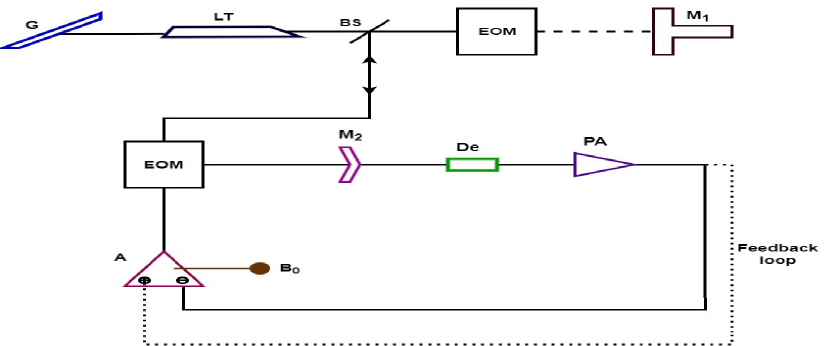
Figure 1: A schematic diagram of a CO₂ laser model: G, diffraction grating; LT, laser tube; BS, beam splitter; EOM, electro-optical modulator; M₁, Piezoelectric (PZT) mirror; M₂, out coupling mirror; De, HgCdTe detector; PA, pre-amplifier; A, differential amplifier, B₀, bias voltage input. The dotted line represents an additional negative feedback which may be used to control chaos of the system.

In Eq. (1), the modulated injected beam is modeled by the term $-k_{0}I\epsilon\cos(\Omega t)$ in which $\epsilon$ is the modulation depth and $\Omega$ is the driving frequency of modulation. By disregarding the term $\propto k_{1}$ and the equation for $V$ [the third equation in Eq. (1)], one can recover the same model as in Ref. perez1994 . Also, in absence of the time-dependent perturbation $\propto\epsilon$, one can reproduce a similar model as in Ref. meucci1997 . Note that both the time-dependent perturbation and the negative feedback driven by $V$ have been separately used to control chaos in different investigations perez1994 ; meucci1997 . In Ref. perez1994 , the intesity decay rate was considered to be a constant, however, in Ref. meucci1997 , the same was modified to involve a constant decay rate plus a voltage dependent perturbation part. The motivation of this work is to propose a modified dynamical system for CO₂ lasers by including both these feedback beams, and to study their interplay and roles for the onset of chaos and hyperchaos. Furthermore, we also construct a network with the hyperchaotic CO₂ lasers as its nodes and study their synchronization. The key parameters for generating chaos and hyperchaos are $\epsilon$ and $B$. However, the absence of any one of them results into chaos instead of hyperchaos in the system.

A schematic diagram of our model for a possible experimental setup is shown in Fig. 1. In this configuration, the leaser beam can be modulated by using (i) a CdTe electro-optic modulator (EOM) and (ii) an intracavity EOM, and can be fed back to the EOMs by a mirror ($M_{1}$) mounted on a piezoelectric transducer (PZT) and an out coupling mirror ($M_{2}$). The intensity of the laser beam can be measured using HgCdTe photodiode detector (De) followed by an amplifier (PA). The CO₂ laser may be driven into chaos by injecting any one of the modulated feedback beams mentioned above. However, an additional negative feedback, to be obtained from subharmonic components of the laser intensity, may be used to establish hyperchaos in the system meucci1997 .

It is useful to define/redefine the dimensionless variables as $x=\alpha I/k_{0},~{}y=\alpha k_{0}/N,~{}z=\pi(V-V_{0})/V_{\lambda},~{}n={\alpha N_{0}}/{k_{0}},~{}b={\pi(V_{0}-B)}/{V_{\lambda}},~{}r={\pi k_{0}R}/{\alpha V_{\lambda}},~{}\zeta=\eta{k_{0}}/{\alpha},~{}\tau=\gamma t$. Also, we set $l_{1}={k_{0}}/{\gamma},~{}l_{2}={\Omega}/{\gamma},~{}l_{3}={k}/{\gamma}$ and $l_{4}={\beta}/{\gamma}$. Thus, equations in (1) reduce to

$$\begin{split}\frac{dx}{d\tau}&=x\left[l_{1}\left(y-1-k_{1}\sin^{2}{z}\right)-l_{3}\epsilon\cos(l_{2}\tau)\right]\\ \frac{dy}{d\tau}&=-(y-n)-2l_{1}xy\\ \frac{dz}{d\tau}&=-l_{4}\left(z-b+\frac{rx}{1+\zeta x}\right).\end{split}$$ (3)

We study the dynamical properties CO₂ lasers given by Eq. (3), and show that the system indeed exhibits chaos and hyperchaos by the control parameters $\epsilon$ and $b$ associated with the modulation depth and the bias voltage. To this end, we first find the equilibrium points of the system which can be obtained by equating the right-hand sides of Eq. (3) to zero and finding solutions for $x,~{}y$ and $z$. Thus, an equilibrium point is obtained as $P(0,n,b)$ $\forall\tau$. The stability of the system (3) about the fixed point $P$ can now be studied. So, we consider the following perturbed system of equations for $X=(x_{1},y_{1},z_{1})$, where $x_{1}=x$, $y_{1}=y-n$ and $z_{1}=z-b$.

$$\begin{split}\frac{dx_{1}}{d\tau}&=x_{1}\left[l_{1}\left(y_{1}+n-1-k_{1}\sin^{2}(z_{1}+b)\right)-l_{3}\epsilon\cos(l_{2}\tau)\right],\\ \frac{dy_{1}}{d\tau}&=-y_{1}-2l_{1}x_{1}(y_{1}+n),\\ \frac{dz_{1}}{d\tau}&=-l_{4}\left(z_{1}+\frac{rx_{1}}{1+\zeta x_{1}}\right).\end{split}$$ (4)

Equation (4) can be rewritten as

$$\dot{X}=A(X,\tau)X,$$ (5)

where $A$ is the coefficient matrix, given by,

$$A=\begin{bmatrix}\phi_{1}&0&0\\ -2l_{1}(y_{1}+n)&-1&0\\ -{rl_{4}}/({1+\zeta x_{1}})&0&-l_{4}\\ \end{bmatrix}.$$ (6)

Here, $\phi_{i}=l_{1}\left(y_{i}+n-1-k_{1}\sin^{2}(z_{i}+b)\right)-l_{3}\epsilon\cos(l_{2}\tau)$ with $i=1$. Next, we assume that Eq. (5) has a solution of the form $X=\Psi(\tau)X(\tau_{0})$ where $X(\tau_{0})$ denotes the initial value of $X=(x_{1},y_{1},z_{1})$ at $\tau=\tau_{0}$ and

$$\Psi(\tau)=I+\int_{\tau_{0}}^{\tau}A(s)ds+\int_{\tau_{0}}^{\tau}A(r)dr\int_{\tau_{0}}^{r}A(s)ds+\cdots,$$ (7)

i.e., $\Psi(\tau)$ is a propagator from the state time $\tau_{0}$ to $\tau$ and is equivalently

$$\Psi(\tau)=\lim_{\delta\tau\rightarrow 0}\Pi_{j=1}^{n}e^{A(\tau_{j})\delta\tau},$$ (8)

where $\tau_{0}=\tau_{1}<\tau_{2}<\tau_{3}<\cdots<\tau_{n-1}<\tau_{n}=\tau$, and $\tau=\tau_{0}+n\delta\tau$ and $\Psi(\tau_{0})=I$, the identity matrix of order $3$. The matrix $\Psi$ describes how a small change in $\tau$ develops from the initial state $X(\tau_{0})$ to the final state $X(\tau)$, and it satisfies the following equation.

$$\frac{d\Psi}{d\tau}=A(\tau)\Psi.$$ (9)

The stability of the system [Eq. (4) or Eq. (5)] can be studied by finding the eigenvalues (Lyapunov exponents) of the matrix, given by,

$$\Lambda=\lim_{\tau\rightarrow\infty}\frac{1}{2\tau}{\log(\Psi^{\text{T}}\Psi)},$$ (10)

where the superscript ‘T’ denotes the transpose of a matrix.

The Lyapunov exponents are shown in Fig. 2 with the variations of the parameters $b$, $\epsilon$ and $r$ for some fixed values of other parameters, i.e., $n=4,~{}l_{1}=28.57,~{}l_{2}=30,~{}l_{3}=25,~{}l_{4}=6.452,~{}k_{1}=2$ and $\zeta=25.57$.

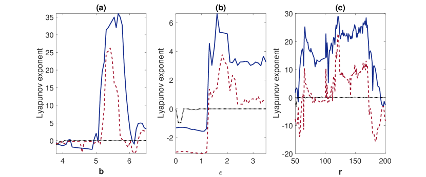
Figure 2: The Lyapunov exponents are shown against the variation of the parameters $b$, $\epsilon$ and $r$. The other parameter values corresponding to the subplots (a), (b) and (c), respectively, are $\epsilon=1.2,~{}r=200$; $b=4.5,~{}r=200$ and $\epsilon=1.2,~{}b=4$.

From Fig. 2, we find that there exist different ranges of values of the parameters in which the system may exhibit periodic, chaotic or hyperchaotic states. In Fig. 2, subplot (a) shows that for some fixed values of $\epsilon=1.2$ and $r=200$, and others remain as above, there is a wide range of values of $b$ for which the two Lyapunov exponents remain positive and another one remains negative. In this case, the periodicity occurs for $0<b<5$, and the chaotic or hyperchaotic states may occur either in $5\lesssim b\lesssim 6.5$ or $b>6.5$. However, from the subplot (b) one can predict that while the periodicity may occur in the range $0<\epsilon\lesssim 1.5$, the hyperchaotic state is more likely to occur for $\epsilon\gtrsim 1.43$ with some fixed values of $b=4.5$ and $r=200$ as at least two Lyaponv exponents assume positive values therein. This means that the injected modulated feedback beam ($\sim\cos\Omega t$) or that associated with the bias voltage $B$ is the prerequisite for the onset of hyperchaos in CO₂ lasers. Furthermore, it is also noticed that the system with chaotic/hyperchaotic states reaches towards a steady state as the value of $r$ increases [subplot (c)]. In order to justify the results of Fig. 2, we also show the bifurcation diagrams corresponding to the parameters $b$, $\epsilon$ and $r$ as in Fig. 3. From the subplot (a), it is clear that there are some ranges of values of $b$ for which the periodicity and chaotic or hyperchaotic states occur one after another. Subplot (b) confirms that the periodicity route to chaos/hyperchaos occurs in some ranges of values of $\epsilon$. Furthermore, the fact that the higher values of $r$ leads to a steady state is evident from the subplot (c).

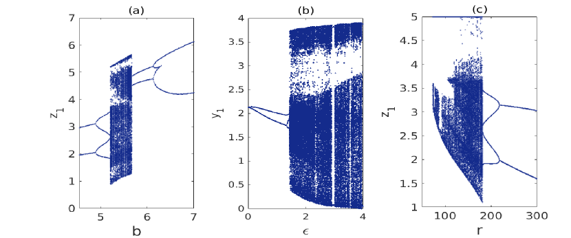
Figure 3: The bifurcation diagrams are shown with respect to the parameters $b$, $\epsilon$ and $r$. The other parameter values corresponding to the subplots (a), (b) and (c) are the same as in Fig. 2.

For an illustration purpose, we plot different phase portraits (Fig. 4) to show that the periodic [subplots (a) and (b)], multi-periodic [subplot (c)], chaotic [subplot (d)] and hyperchaotic [subplot (e)] states of the system coexist for different ranges of values of the parameters, especially $b,~{}\epsilon$ and $r$.

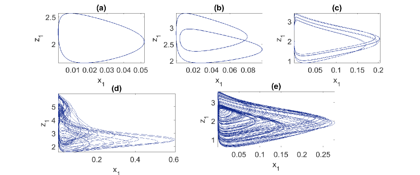
Figure 4: Different phase portraits are shown with the variation of the parameter $\epsilon$: (a) stable and single periodic orbit $(\epsilon=1.2)$ (b) stable and double periodic orbit $(\epsilon=1.4)$ (c) unstable and multi-periodic orbit $(\epsilon=1.54)$ (d) chaotic orbit $(\epsilon=1.7)$ and (e) hyperchaotic orbit $(\epsilon=2)$. The other parameter values are $b=4.5,~{}r=200$, $n=4,~{}l_{1}=28.57,~{}l_{2}=30,~{}l_{3}=25,~{}l_{4}=6.452,~{}k_{1}=2$ and $\zeta=25.57$.

III Network of coupled hyperchaotic CO₂ lasers and synchronization

We construct a network graph in which each edge of the graph is connected to a finite number of nodes. We choose the hyperchaotic CO₂ lasers, given by Eq. (3), as the nodes or oscillators, and couple them through the $x$ and $y$ variables. Here, the coupling with the $z$ variable is not introduced as it corresponds to the voltage obtained through a feedback loop. Next, we derive a variational equation from the coupled set of equations and study the stability of the synchronous state of the coupled oscillators using the method of MSF. A numerical simulation approach is also performed to find the synchronization errors and to validate the theory of MSF for a finite number of nodes.

The network of $n$ identical oscillators that are linearly coupled are given by

$$\begin{split}\frac{dx_{i}}{d\tau}&=x_{i}\left[l_{1}\left(y_{i}-1-k_{1}\sin^{2}{z_{i}}\right)\right]-l_{3}\epsilon\cos(l_{2}\tau)\\ &+\sigma_{1}\sum_{j=1}^{n}G_{ij}x_{j},\\ \frac{dy_{i}}{d\tau}&=-(y_{i}-n)-2l_{1}x_{i}y_{i}+\sigma_{2}\sum_{j=1}^{n}G_{ij}y_{j},\\ \frac{dz_{i}}{d\tau}&=-l_{4}\left(z_{i}-b+\frac{rx_{i}}{1+\zeta x_{i}}\right),\end{split}$$ (11)

which can be rewritten in the following form.

$$\dot{X}_{i}=F(X_{i})+\sigma\sum_{j}G_{ij}X_{j}.$$ (12)

Here, $X_{i}=(x_{i},y_{i},z_{i})$ denotes the three-dimensional vector of the dynamical variables (corresponding to $x,~{}y$ and $z$) of the $i$th node, $\sigma=(\sigma_{1},\sigma_{2},0)$ is the coupling strength, and $G=(G_{ij})_{n\times n}$ is a Laplacian matrix of order $n$ with zero row-sums (i.e., $\sum_{j}G_{ij}=0$ such that the synchronization manifold, defined by the $n-1$ constraints $X_{1}=X_{2}=\cdots=X_{n}$, is an invariant manifold) and non-negative off diagonal elements. For different choice of the matrix $G$, one can have different connectivity of nodes. For example, $G=G_{1}$ or $G_{2}$ according to when one considers the RDC or SC networks where pecora1998 ; belykh2004

$$G_{1}=\begin{bmatrix}-2&1&0&0&...&1\\ 1&-2&1&0&...&0\\ 0&1&-2&1&...&0\\ ...&...&...&...&...&...\\ 1&0&0&...&1&-2\end{bmatrix}$$ (13)

and

$$G_{2}=\begin{bmatrix}-(n-1)&1&1&1&...&1\\ 1&-1&0&0&...&0\\ 1&0&-1&0&...&0\\ ...&...&...&...&...&...\\ 1&0&0&...&0&-1\end{bmatrix}.$$ (14)

Next, we combine the matrices $G_{1}$ and $G_{2}$ with the coupling strengths $\sigma_{1}$ and $\sigma_{2}$ to obtain the corresponding matrices $H=H_{1}$ and $H=H_{2}$ which contain $3\times 3$ matrix blocks, so that Eq. (12) can be recast as

$$\dot{X_{i}}=F(X_{i})+\sum_{j}H_{ij}X_{j},$$ (15)

. where $H=(H_{ij})_{n\times n}$. Thus, for $n$ nodes or oscillators we get the matrices $H_{1}$ and $H_{2}$ of order $3n$:

$$H_{1}=\begin{bmatrix}-2J_{3}&J_{3}&O_{3}&...&O_{3}&J_{3}\\ J_{3}&-2J_{3}&J_{3}&...&O_{3}&O_{3}\\ O_{3}&J_{3}&-2J_{3}&...&O_{3}&O_{3}\\ ...&...&...&...&...&...\\ ...&...&...&...&...&...\\ -2J_{3}&O_{3}&O_{3}&...&J_{3}&-2J_{3}\end{bmatrix},$$ (16)

and

$$H_{2}=\begin{bmatrix}(-n+1)J_{3}&J_{3}&J_{3}&.....&J_{3}&J_{3}\\ J_{3}&-J_{3}&O_{3}&.....&O_{3}&O_{3}\\ J_{3}&O_{3}&-J_{3}&.....&O_{3}&O_{3}\\ ...&...&...&.....&...&....\\ ...&...&...&.....&...&....\\ -J_{3}&O_{3}&O_{3}&.....&O_{3}&-J_{3}\end{bmatrix}$$ (17)

with $O_{3}$ denoting the null matrix of order $3$ and

$$J_{3}=\begin{bmatrix}\sigma_{1}&0&0\\ 0&\sigma_{2}&0\\ 0&0&0\end{bmatrix}.$$ (18)

In order to study the synchronization of $n$ coupled oscillators, given by Eq. (15) and its stability, we decompose them into driving and response systems, i.e., we assume the driving system as

$$\begin{split}\dot{x_{i}}=&f_{1}(x_{i},y_{i},z_{i}),\\ \dot{y_{i}}=&f_{2}(x_{i},y_{i},z_{i}),\\ \dot{z_{i}}=&f_{3}(x_{i},y_{i},z_{i}),\end{split}$$ (19)

and the response system as

$$\begin{split}\dot{x_{j}}=&f_{1}(x_{j},y_{j},z_{j}),\\ \dot{y_{j}}=&f_{2}(x_{j},y_{j},z_{j}),\\ \dot{z_{j}}=&f_{3}(x_{j},y_{j},z_{j}),\end{split}$$ (20)

where $i,j=1,2,...,n$ and $i\neq j$, and the functions $f_{1},~{}f_{2}$ and $f_{3}$ represent the right-hand sides of Eq. (11). Here, we note that for the $z$ variable, no coupling strength is considered for the reason mentioned before. Also, in the process of synchronization, we must have $\parallel(x_{i+1},y_{i+1},z_{i+1})-(x_{i},y_{i},z_{i})\parallel\longrightarrow 0$ as $t\longrightarrow\infty$. So, synchronization of $n$ identical nodes, given by Eq. (15), can be studied by considering the evolution of the variations $\xi_{i}^{1}=x_{i+1}-x_{i},~{}\xi_{i}^{2}=y_{i+1}-y_{i},~{}\xi_{i}^{3}=z_{i+1}-z_{i}=0$ for $i=1,2,...,n-1$ and $\xi_{n}^{1}=x_{n}-x_{1},~{}\xi_{n}^{2}=y_{n}-y_{1},~{}\xi_{n}^{3}=z_{n}-z_{1}$. Thus,

$$\begin{split}\dot{\xi}_{i}^{1}=&f_{1}(x_{i+1},y_{i+1},z_{i+1})-f_{1}(x_{i},y_{i},z_{i}),\\ \dot{\xi}_{i}^{2}=&f_{2}(x_{i+1},y_{i+1},z_{i+1})-f_{2}(x_{i},y_{i},z_{i}),\\ \dot{\xi}_{i}^{3}=&0,\end{split}$$ (21)

or,

$$\begin{split}\dot{\xi}_{i}^{1}=&f_{1}(x_{i}+\xi_{i}^{1},y_{i}+\xi_{i}^{2},z_{i})-f_{1}(x_{i},y_{i},z_{i}),\\ \dot{\xi}_{i}^{2}=&f_{2}(x_{i}+\xi_{i}^{1},y_{i}+\xi_{i}^{2},z_{i})-f_{2}(x_{i},y_{i},z_{i}),\\ \dot{\xi}_{i}^{3}=&0.\end{split}$$ (22)

In what follows, we Taylor expand the functions $f_{1}$ and $f_{2}$ about $(x_{i},y_{i},z_{i})$ and keep terms up to the first orders of $\xi_{i}^{1}$ and $\xi_{i}^{2}$ to obtain for $i=1,2,...,n$ the following equation.

$$\begin{bmatrix}\dot{\xi}_{i}^{1}\\ \dot{\xi}_{i}^{2}\\ \dot{\xi}_{i}^{3}\end{bmatrix}=\begin{bmatrix}\frac{\delta f_{1}}{\delta x}&\frac{\delta f_{1}}{\delta y}&0\\ \frac{\delta f_{2}}{\delta x}&\frac{\delta f_{2}}{\delta y}&0\\ 0&0&0\end{bmatrix}\begin{bmatrix}\xi_{i}^{1}\\ \xi_{i}^{2}\\ \xi_{i}^{3}\end{bmatrix}.$$ (23)

Thus, a variational equation of Eq. (15) is obtained as

$$\dot{\xi}=(F+H\otimes E)\xi,$$ (24)

where $\xi=(\xi_{1}^{1},\xi_{1}^{2},\xi_{1}^{3};\xi_{2}^{1},\xi_{2}^{2},\xi_{2}^{3},...,\xi_{n}^{1},\xi_{n}^{2},\xi_{n}^{3})$, $E$ and $F$ are the matrices (each of order $3n$), given by,

$$E=\begin{bmatrix}P&O_{3}&O_{3}&...&O_{3}\\ O_{3}&P&O_{3}&...&O_{3}\\ ...&...&...&...&...\\ O_{3}&O_{3}&O_{3}&...&P\end{bmatrix},~{}F=\begin{bmatrix}F_{1}&O_{3}&O_{3}&...&O_{3}\\ O_{3}&F_{2}&O_{3}&...&O_{3}\\ ...&...&...&...&...\\ O_{3}&O_{3}&O_{3}&...&F_{n}\end{bmatrix},$$ (25)

with

$$P=\begin{bmatrix}1&0&0\\ 0&1&0\\ 0&0&0\end{bmatrix},~{}F_{i}=\begin{bmatrix}\phi_{i}&l_{1}x_{i}&0\\ -2l_{1}(y_{i}+n)&-1-2l_{1}x_{i}&0\\ 0&0&0\end{bmatrix}$$ (26)

for $i=1,2,...,n$. Also, in Eq. (24), $H$ is $H_{1}$ or $H_{2}$ according to when we choose RDC or SC networks.

III.1 Stability analysis of synchronous states

The master stability function, which relies on finding the maximum Lyapunov exponent for the least stable transverse mode of the synchronization manifold along with the eigenvalues of the connectivity matrix, has been recognized as one of the most powerful tools for determining the stability of synchronous states of linearly coupled oscillators pecora1998 . Such MSF allows one to quickly establish whether any linear coupling of oscillators will result into a stable synchronous dynamics. It also reveals which desynchronization bifurcation mode will occur due to changes of the coupling scheme or strength. Furthermore, it simplifies a large-scale networking system to a node-size system via diagonalization and decoupling as long as the inner coupling functions for all node pairs are identical.

We recall the variational equation (24), which will be used to calculate the Lyapunov exponents, as

$$\dot{\xi}=(F+H\otimes E)\xi,$$ (27)

We note that in Eq. (27) the matrix $F$ is a block diagonal matrix which involves $3\times 3$ block matrices $F_{i}$. The matrix $H\otimes E$ can be treated by diagonalizing the symmetric matrix $H$ (i.e., $H_{1}$ or $H_{2}$) as $E$ is already a diagonal matrix. Thus, a block diagonalized variational equation can be formed with each block having the form

$$\dot{\xi}_{k}=(F_{k}+\lambda_{k}P)\xi_{k},$$ (28)

where $\lambda_{k}$ is an eigenvalue of a block diagonal $3\times 3$ matrix element of $H$ with $k=0,1,2$. There are, in fact, $n$ equations of the form of Eq. (28) and, in general, the eigenvalues $\lambda_{k}$ for each diagonal $3\times 3$ block matrix element of $H$ will be different from the other blocks. The equation with $k=0$ where $\lambda_{0}=0$ corresponds to the variational equation for the synchronization manifold defined by $X_{1}=X_{2}=\cdots=X_{n}$. So, there are $3n$ eigenvalues for $n$ numbers of $3\times 3$ blocks of which at least $n$ eigenvalues are zero. The maxima $\gamma^{\text{max}}_{i},~{}i=1,2,...,n$, of the Lyapunov exponents are obtained for each block variational equation (28), and finally, the maximum of these maxima, i.e., $\gamma_{\text{max}}=\text{max}_{i}\{\gamma^{\text{max}}_{i}\}$ ($n$ times) is obtained as the MSF of the variational equation (27) with the coupling parameters $\sigma_{1}$ and $\sigma_{2}$. If $\gamma_{\text{max}}<0$, the synchronous state is said to be stable at the coupling strengths, otherwise, it is unstable for $\gamma_{\text{max}}>0$.

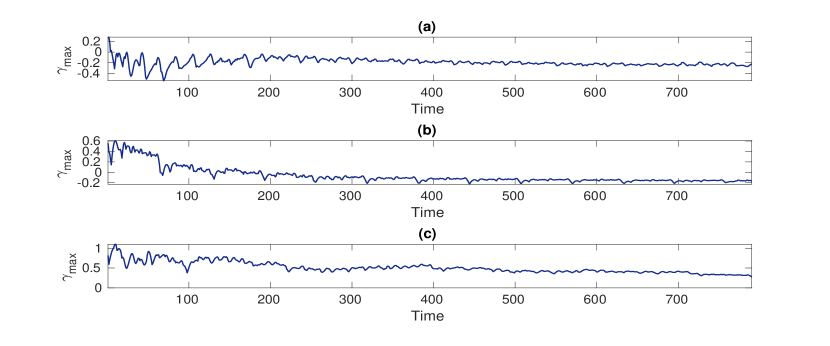
Figure 5: The maximum Lyapunov exponent of the variational equation (28) is shown for nearest-neighbor ring of diffusive coupling (RDC) networks with different number of nodes: (a) $20$, (b) $24$ and (c) $28$. The coupling parameters are $\sigma_{1}=28$ and $\sigma_{2}=26$.

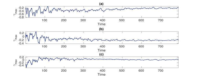
Figure 6: The same as in Fig. 5, but for star coupling (SC) networks with (a) $20$, (b) $24$ and (c) $28$ nodes. The coupling parameters are $\sigma_{1}=5$ and $\sigma_{2}=3.2$.

We numerically calculate the Lyapunov exponents of the variational equation (28) as functions of $\sigma_{1}$ and $\sigma_{2}$ for both the RDC and SC networks with different number of nodes. The corresponding maxima of these exponents $(\gamma_{\text{max}})$ are plotted against time for (a) $20$, (b) $24$ and (c) $28$ nodes as shown in Figs. 5 and 6. We find that given a coupling strength, the Lyapunov exponent, $\gamma_{\text{max}}<0$ in a bounded region for a longer time for both types of networks with at most $24$ number of nodes [as $\gamma_{\text{max}}>0$ for $n>24$, see, e.g., subplot (c) for $n=28$], implying that the synchronous state reaches a steady state at that coupling strength. However, while lower values of $\sigma_{1},~{}\sigma_{2}~{}\sim o(1)$ can lead to the stable synchronization for SC networks (Fig. 6), relatively higher coupling strengths are required for the RDC networks (Fig. 5). A schematic diagram for the synchronization of both the RDC and SC networks with $20$ nodes is shown in Fig. 7.

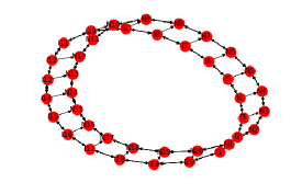
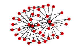
Figure 7: A schematic diagram for the synchronization of $20$ nodes in a ring of diffusively coupled [subplot (a)] and start coupled [subplot (b)] networking system.

III.2 Synchronization and chimera states

In order to validate our results in Sec. III.1, we employ the Runge-Kutta scheme to calculate the synchronization errors corresponding to different sets of (e.g., $n=20$, $24$ and $28$) coupled equations, given by Eq. (11), that exhibit hyperchaos. The simulation results are displayed in Figs. 8 and 9. These basically represent the synchronization errors between the laser intensities of different nodes, i.e., $x_{i+1}-x_{i}$ at the hyperchaotic states. We find that the synchronization of the coupled oscillators is achieved through the inclusion of the coupling terms $\propto\sigma$ and the corresponding errors for the intensities of the $i+1$-th and $i$-th nodes are $\lesssim 10^{-12}$, $10^{-6}$ or $10^{-5}$ according to when we choose $n=20$, $24$ or $28$ nodes. Thus, from the results as in Figs. 5 and 6, and 8 and 9, we can conclude that the synchronization in networks of hyperchaotic CO₂ lasers can be possible for at most $24$ nodes as evident from the sign of the maximum Lyapunov exponent ,i.e., $\gamma_{\text{m}ax}<0$ and the synchronization error $\lesssim 10^{-6}$.

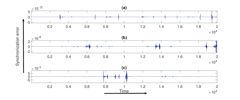
Figure 8: Synchronization error ($||\xi||$) is shown with respect to time ($\tau$) for (a) $20$ (b)$24$ and (c) $28$ nodes in a ring coupling network. The coupling parameters are $\sigma_{1}=28$ and $\sigma_{2}=26$.

.

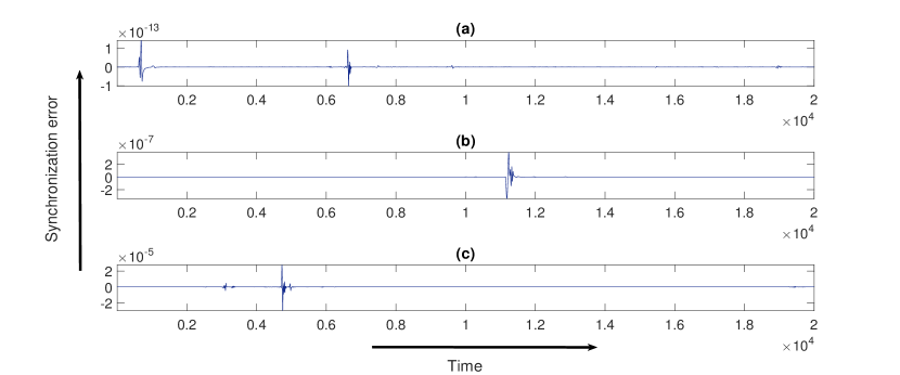
Figure 9: Synchronization error ($||\xi||$) is shown with respect to time ($\tau$) for (a) $20$ (b)$24$ and (c) $28$ nodes in a star coupling network. The coupling parameters are $\sigma_{1}=5$ and $\sigma_{2}=3.2$

.

From the characteristics of the Lyapunov exponents (Figs. 5 and 6) and the synchronization errors (Figs. 8 and 9) we conclude that the steady states of synchronizations of RDC and SC networks (with synchronization error $\lesssim 10^{-6}$) can be reached with at most $24$ number of nodes. However, the chimera states in the networks may coexist in some time intervals where the synchronization does not occur for both the RDC and SC networks. In order to clarify it, we plot the synchronization errors against the coupling parameters $\sigma_{1}$ and $\sigma_{2}$ as shown in Figs. 10 and 11. It is evident that while the synchronization in RDC networks occurs for some higher values of $\sigma_{1}$ and $\sigma_{2}$, i.e., $26\lesssim\sigma_{1}\lesssim 40$ [Fig. 10 (a)] and $20\lesssim\sigma_{2}\lesssim 35$ [Fig. 10 (b)], the same for SC networks occurs at lower values of $\sigma_{1}$ and $\sigma_{2}$, i.e., $2.3\lesssim\sigma_{1}\lesssim 6.6$ [Fig. 11 (a)] and $0<\sigma_{2}\lesssim 6$ [Fig. 11 (b)]. In the other intervals, the chimera states may be formed.

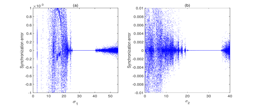
Figure 10: Synchronization errors ($||\xi||$) are plotted against the coupling parameters (a) $\sigma_{1}$ and (b)$\sigma_{2}$ to show that the chimera states exist in a RDC network with $24$ nodes.

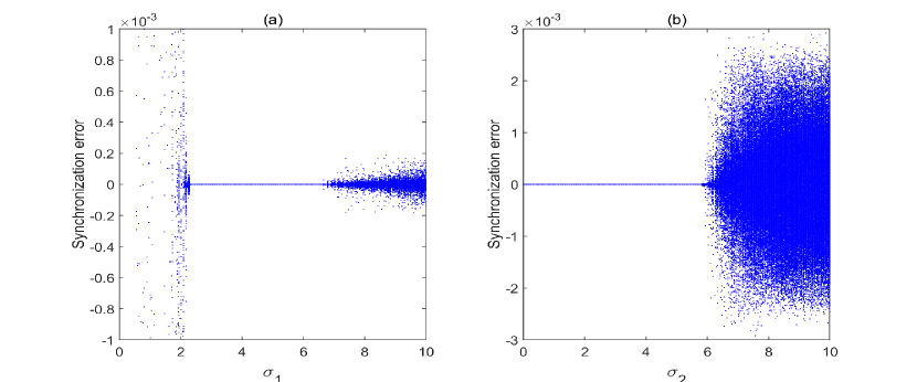
Figure 11: Synchronization errors ($||\xi||$) are plotted against the coupling parameters (a) $\sigma_{1}$ and (b)$\sigma_{2}$ to show that the chimera states exist in a SC network with $24$ nodes.

IV Discussion and Conclusion

We have proposed a non-autonomous dynamical system for an optically modulated CO₂ laser in presence of electro-optic feedback beams: one in the form of a small-amplitude time-dependent perturbation and the other a negative feedback of subharmonic components of the laser intensity signal. A numerical study of the dynamical system reveals that the feedback beams can indeed drive the CO₂ lasers into hyperchaotic states. The periodic, multi-periodic and chaotic states of the laser are also found to coexist for different values of the key parameters $B$, $\epsilon$ and $R$ associated with, respectively, the bias voltage, the modulation depth of the feedback beam and the gain from the feedback loop. A network of a finite number of hyperchaotic coupled CO₂ lasers as its nodes or oscillators is constructed with linear coupling strengths, and its synchronization is studied by the method of master stability function pecora1998 . It is found that a network of at most $24$ identical oscillators may be fully synchronized (where $\gamma_{\text{max}}<0$) both in the star and ring of diffusively coupled networks. In both these cases, the synchronization errors, as obtained from numerical simulation of $24$ coupled hyperchaotic CO₂ lasers, are $\lesssim 10^{-6}$. It is also found that, while the lower coupling strengths $\sim o(1)$ can lead to a synchronous state of star networks, relatively higher coupling strengths are required for the nearest-neighbor diffusive (ring) networks.

It is to be noted that in our network model, we have considered only the ring of diffusively coupled (RDC) and star coupling (SC) networks. However, different other networks can be constructed, e.g., by combining both these ring and star networks, and their synchronization can be studied following the present stability analysis. In this case, the matrix $G$, and so $G_{1}$ and $G_{2}$ may not be the same as the present ones. Also, the numbers $n=20,~{}24$ and $28$ does not have any particular meaning. These are considered arbitrarily. In fact, one can consider any number of modes to examine the synchronization in networks. In our theory, we have seen that the synchronization error becomes higher $(\gtrsim 10^{-6})$ for $n>24$. For illustrations, we have examined the synchronization with different number of nodes, i.e., $n=20,~{}24$ and $28$ to obtain the synchronization errors as $\sim 10^{-12},~{}10^{-6}$ and $10^{-5}$ respectively. Furthermore, the chimera states of the networks may coexist in some intervals of time and the coupling parameters $\sigma_{1}$ and $\sigma_{2}$ where the networks are not synchronized. This means that the synchronization occurs only in some specific ranges of values of $\sigma_{1}$ and $\sigma_{2}$, namely, $26\lesssim\sigma_{1}\lesssim 40$ and $20\lesssim\sigma_{2}\lesssim 35$ for RDC networks, and $2.3\lesssim\sigma_{1}\lesssim 6.6$ and $0<\sigma_{2}\lesssim 6$ for SC networks. However, the detailed discussion about the formation of chimera states is beyond the scope of the present work.

In the present network model, each node is connected to independent but identical CO₂ lasers which exhibit hyperchaos. Since in the process of synchronization, all the connected nodes behave in a similar manner, one can use this property of RDC and SC networks to produce a secure networking communication system in which the sender hides a message within the hyperchaotic signal that can only be recovered by the receiver at the synchronized state. Such an approach has been extensively applied in many secure communications, especially in optical chaos communication systems because of the added security and the speed of optical communications parlitz1996 . In this way, one can also develop the public key cryptography scheme using the process of chaos synchronization which reduces the difficulties of the problems of key distribution in an encryption process banerjee2011 ; roy2019 ; li2019b .

Recently, a different approach other than the MSF scheme has been proposed in Ref. abarbanel2008 , however, the method has some limitations, and we are not sure whether this method can be successfully applied to the present model to examine the synchronization in networks of CO₂ lasers. It requires further investigation which is beyond the scope of the present work. Also, the theory of phase synchronization has been extended to chaotic model oscillators and to several laser experiments. In this context, the synchronization in presence of noise which usually has a destructive effect on phase synchronization by inducing phase slips and shrinking the synchronization region may be interesting to study zhou2003 . The inclusion of the time delay effect of the light being fed back to the cavity, and also the laser field phase in the present model may be other problems of interest.

To conclude, the synchronization phenomena in our network of hyperchaotic lasers may be applicable to neural networks which are information processing paradigms inspired by the way biological neural systems process data.

References

References

- (1) Bonatto C, Garreau J C and Gallas J A C 2005 Phys. Rev. Lett. 95 143905.
- (2) Arecchi F T, Meucci R, Puccioni G and Tredicce J 1982 Phys. Rev. Lett. 49 1217.
- (3) Olson G J, Mocker H W, Demma N A and Ross J B 1995 Appl. Optics 34 2033.
- (4) Billings L, Schwartz I B, Morgan D S, Bollt E M, Meucci R and Allaria E 2004 Phys. Rev. E 70 026220.
- (5) Liu S, Wang Y and Li B 2014 IEEE Seventh International Symposium on Computational Intelligence and Design, DOI: 10.1109/ISCID.2014.232.
- (6) Jiang C, Liu Y, Zhao Y, Mou C, Wang T 2019 J. Lightwave Tech., 37 889. DOI: 10.1109/JLT.2018.2883376.
- (7) Gilmore R and Lefranc M 2002 The Topology of Chaos, Alice in Stretch and Squeezeland (Wiley, New York); Gilmore R 1998 Rev. Mod. Phys. 70 1455.
- (8) Pisarchik A, Meucci R and Arecchi F 2001 Eur. Phys. J. D 13 385.
- (9) Perez J M, Steinshnider J, Stallcup R E and Aviles A F 1994 Appl. Phys. Lett. 65 1216.
- (10) Ciofini M, Labate A, Meucci R and Galanti M 1999 Phys. Rev. E 60 398.
- (11) Meucci R, Labate A and Ciofini M 1997 Phys. Rev. E 56 2829.
- (12) Ott E, Grebogi C and Yorke J A 1990 Phys. Rev. Lett. 64 1196.
- (13) Hunt E R 1991 Phys. Rev. Lett. 67 1953.
- (14) Pecora L M and Carroll T L 1990 Phys. Rev. Lett. 64 821.
- (15) Kocarev L and Parlitz U 1995 Phys. Rev. Lett. 74 5028.
- (16) Parlitz U, Kocarev L, Stojanovski T and Preckel H 1996 Phys. Rev. E 53 4351.
- (17) Militello B et al 2018 Phys. Scr. 93 025201.
- (18) Hu T and Sun W 2013 Phys. Scr. 87 015001.
- (19) Zheng S and Bi Q 2011 Phys. Scr. 84 025008.
- (20) Li C, Qiani K, He S, Li H and Feng W 2019 IEEE Access 7, 160072.
- (21) Li C-L, Li H-M, Li W, Tong Y-N, Zhang J, Wei D-Q and Li F-D 2018 Int. J. Electro. Commun. 84 199.
- (22) He S, Sun K, Wang H, Mei X and Sun Y 2018 Nonlinear Dynamics 92, 85.
- (23) He S, Sun K and Wang H 2016 Eur. Phys. J. Spl. Topic. 225, 97.
- (24) Somers D and Kopell N 1995 Phys. D 89 169.
- (25) Heagy J F, Carroll T L and Pecora L M 1994 Phys. Rev. E 50, 1874.
- (26) Heagy J F, Carroll T L and Pecora L M 1994 Phys. Rev. Lett.74 4185.
- (27) Barahona M and Pecora L M 2002 Phys. Rev. Lett. 89 054101.
- (28) Tang L et al. 2019 Phys. Rev. E 99 012304.
- (29) Karimi S et al 2019 Phys. Scr. 94 105215.
- (30) Belykh V N, Belykh I and Hasler M 2004 Physica D: Nonlinear Phenomena 195 159.
- (31) Pecora L M and Carroll T L 1998 Phys. Rev. Lett. 80 2109.
- (32) Banerjee S, Rondoni L, Mukhopadhyay S and Misra A P 2011 Opt. Commun. 284 2278.
- (33) Roy A, Misra A P and Banerjee S 2019 Optik 176 119.
- (34) Li C-L, Li Z-Y, Feng W, Tong Y-N, Du J-R and Wei D-Q 2019 Int. J. Electro. Commun. 110 152861.
- (35) Abarbanel H D I, Creveling D R and Jeanne J M 2008 Phys. Rev. E 77 14.
- (36) Zhou C S, Kurths J, Allaria E, Boccaletti S, Meucci R and Arecchi F T 2003 Phys. Rev. E 67 015205(R).