Re-examination of the rare decay $B_{s}\to\phi\mu^{+}\mu^{-}$ using holographic light-front QCD

Abstract

We calculate the Standard Model (SM) predictions for the differential branching ratio of the rare $B_{s}\to\phi\mu^{+}\mu^{-}$ decays using $B_{s}\to\phi$ transition form factors (TFFs) obtained using holographic light-front QCD (hQCD) instead of the traditional QCD sum rules (QCDSR) . Our predictions for the differential branching ratio is in better agreement with the LHCb data. Also, we find that the hQCD prediction for $R_{K^{*}\phi}$, the ratio of the branching fraction of $B\to K^{*}\mu^{+}\mu^{-}$ to that of $B_{s}\to\phi\mu^{+}\mu^{-}$ , is in excellent agreement with both the LHCb and CDF results in low $q^{2}$ range.

I Introduction

The flavor changing neutral current (FCNC) $b\to s$ transition, which is forbidden at tree-level, has been at the focus of extensive experimental and theoretical investigations. This is due to the fact that, among other things, this rare transition is sensitive to New Physics (NP), i.e. physics beyond the Standard Model (SM). In extensions of the SM, new heavy particles can appear in competing diagrams and affect both the branching fraction of the decay and the angular distributions of the final-state particles. In particular, the semi-leptonic $b\to s\ell^{+}\ell^{-}$quark decay has received significant attention via measurements of inclusive $B\to X_{s}\ell^{+}\ell^{-}$ and exclusive $B\to K\mu^{+}\mu^{-}$ and $B\to K^{*}\mu^{+}\mu^{-}$ decays and their comparison against the SM predictions. Many observables for the dileptonic $B\rightarrow K^{*}\mu^{+}\mu^{-}$decay have already been measured and the precision of the experimental data is expected to improve significantly in the near future. The decay $B_{s}\to\phi\mu^{+}\mu^{-}$ , which is closely related to the decay $B\to K^{*}\mu^{+}\mu^{-}$ , provides an alternate venue to examine the same underlying quark process, as shown in Fig.1, in a different hadronic environment.

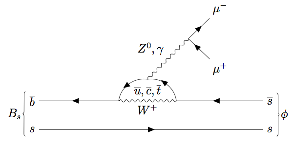
(a) Penguin diagram

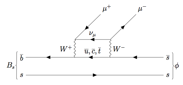
(b) Box diagram

Figure 1: Feynman diagrams of the principal contributions to the $B_{s}\to\phi\mu^{+}\mu^{-}$ decay.

This decay channel was first observed and studied by the CDF collaboration Aaltonen et al. (2011a, b) and subsequently studied by the LHCb collaboration using data collected during 2011, corresponding to an integrated luminosity of $1.0$ fb^-1 Aaij et al. (2013a). Although $B_{s}$ meson production is suppressed with respect to the $B_{d}$ meson by the fragmentation fraction ratio $f_{s}/f_{d}\sim 1/4$, the narrow $\phi$ resonance allows a clean selection with low background levels. While the angular distributions were found to be in good agreement with SM expectations, the measured branching fraction deviates from the recently updated SM prediction by $3.1\,\sigma$ Altmannshofer and Straub (2015); Aaij et al. (2015); Bharucha et al. (2016); Geng and Liu (2003):

$$\frac{d~{}}{dq^{2}}{\rm BR}(B_{s}\to\phi\mu^{+}\mu^{-}){\Big{|}}_{q^{2}\in[1\mathrel{\mathop{\mathchar 58\relax}}6]\,{\rm GeV}^{2}}=\left\{\begin{array}[]{lcl}\displaystyle\left(2.58^{+0.33}_{-0.31}\pm 0.08\pm 0.19\right)\times 10^{-8}~{}{\rm GeV}^{-2}&&({\rm exp.})\\[8.61108pt] \displaystyle\left(4.81\pm 0.56\right)\times 10^{-8}~{}{\rm GeV}^{-2}&&({\rm SM})\,,\end{array}\right.$$ (1)

where $q^{2}=m^{2}_{\mu\mu}$ is the invariant mass of the produced di-muons. A similar trend is also seen for the branching fractions of other $b\to s\mu^{+}\mu^{-}$ processes, which tend to be lower than the SM predictions Aaij et al. (2013b, 2014a, 2014b).

One important aspect of SM theoretical predictions of the exclusive decays is the computation of the TFFs which parametrize the hadronic matrix elements of $B_{(s)}$ to light mesons through quark currents. These nonperturbative TFFs are commonly evaluated using light-cone sum rules (LCSR)Ali et al. (1994) with the input distribution amplitudes (DAs) obtained via QCDSR. An alternative is to calculate these DAs using the light-front wavefunction of the light meson bound state. In a recent work, we have shown that the light-front wavefunctions for $\rho$ and $\phi$ mesons resulting from hQCD leads to predictions for diffractive production cross sections of these vector mesons that are in good agreement with the experimental dataAhmady et al. (2016). This is our motivation to use the hQCD DAs to calculate the $B_{s}\to\phi$ TFFs and consequently, provide alternative predictions for the $B_{s}\to\phi\mu^{+}\mu^{-}$ differential branching ratio. The nonperturbative TFFs are the dominant source of the theoretical uncertainty in this decay mode and therefore it is important to improve our understanding of the corresponding error by examining viable models.

II Holographic meson wavefunctions

In recent years, new insights about hadronic light-front wavefunctions based on the anti-de Sitter/Conformal Field Theory (AdS/CFT) correspondence have been proposed by Brodsky and de Téramond de Teramond and Brodsky (2005); Brodsky and de Teramond (2006); de Teramond and Brodsky (2009). In a semiclassical approximation of light-front QCD where quark masses and quantum loops are neglected, the meson wavefunction can be written as Brodsky et al. (2015)

$$\Psi(x,\zeta,\phi)=e^{iL\phi}\mathcal{X}(x)\frac{\phi(\zeta)}{\sqrt{2\pi\zeta}}$$ (2)

where the variable $\zeta=\sqrt{x(1-x)}r$ is the transverse separation between the quark and the antiquark at equal light-front time. The transverse wavefunction $\phi(\zeta)$ is a solution of the so-called holographic light-front Schrödinger equation:

$$\left(-\frac{d^{2}}{d\zeta^{2}}-\frac{1-4L^{2}}{4\zeta^{2}}+U(\zeta)\right)\phi(\zeta)=M^{2}\phi(\zeta)$$ (3)

where $M$ is the mass of the meson and $U(\zeta)$ is the confining potential which at present cannot be computed from first-principles in QCD. On the other hand, making the substitutions $\zeta\to z$ where $z$ being the fifth dimension of AdS space, together with $L^{2}-(2-J)^{2}\to(mR)^{2}$ where $R$ and $m$ are the radius of curvature and mass parameter of AdS space respectively, Eq. (3) describes the propagation of spin-$J$ string modes in 5-D AdS space. In this case, the potential is given by

$$U(z,J)=\frac{1}{2}\varphi^{\prime\prime}(z)+\frac{1}{4}\varphi^{\prime}(z)^{2}+\left(\frac{2J-3}{4z}\right)\varphi^{\prime}(z)$$ (4)

where $\varphi(z)$ is the dilaton field which breaks the conformal invariance of AdS space. A quadratic dilaton ($\varphi(z)=\kappa^{2}z^{2}$) profile results in a harmonic oscillator potential in physical spacetime:

$$U(\zeta,J)=\kappa^{4}\zeta^{2}+\kappa^{2}(J-1)\;.$$ (5)

The choice of a quadratic dilaton is dictated by the de Alfaro, Furbini and Furlan (dAFF)de Alfaro et al. (1976) mechanism for breaking conformal symmetry in the Hamiltonian while retaining the conformal invariance of the actionBrodsky et al. (2013). Solving the holographic Schrödinger equation with this harmonic potential given by Eq. (5) yields the meson mass spectrum,

$$M^{2}=4\kappa^{2}\left(n+L+\frac{S}{2}\right)\;$$ (6)

with the corresponding normalized eigenfunctions

$$\phi_{n,L}(\zeta)=\kappa^{1+L}\sqrt{\frac{2n!}{(n+L)!}}\zeta^{1/2+L}\exp{\left(\frac{-\kappa^{2}\zeta^{2}}{2}\right)}L_{n}^{L}(x^{2}\zeta^{2})\;.$$ (7)

To completely specify the holographic wavefunction given by Eq. (2), the longitudinal wavefunction $\mathcal{X}(x)$ must be determined. For massless quarks, this is achieved by an exact mapping of the pion electromagnetic form factors in AdS and in physical spacetime resulting in Brodsky et al. (2015).

$$\mathcal{X}(x)=\sqrt{x(1-x)}$$ (8)

Equation (6) predicts that the mesons lie on linear Regge trajectories as is experimentally observed and thus $\kappa$ can be chosen to fit the Regge slope. Ref. Brodsky et al. (2015) reports $\kappa=0.54$ GeV for vector mesons. Eq. (6) also predicts that the pion and kaon (with $n=0,L=0,S=0$) are massless. For the ground state mesons with $n=0,L=0$, Eq. (2) becomes

$$\Psi(x,\zeta)=\frac{\kappa}{\sqrt{\pi}}\sqrt{x(1-x)}\exp{\left[-{\kappa^{2}\zeta^{2}\over 2}\right]}\;.$$ (9)

To account for non-zero quark masses, we follow the prescription of Brodsky and de Téramond given in Ref. Brodsky and de Teramond (2009) which leads to an augmented form for the transverse part of the light-front wavefunction:

$$\Psi^{\phi}_{\lambda}(x,\zeta)=\mathcal{N}_{\lambda}\sqrt{x(1-x)}\exp{\left[-{\kappa^{2}\zeta^{2}\over 2}\right]}\exp{\left[-{m_{s}^{2}\over 2\kappa^{2}x(1-x)}\right]}\,,$$ (10)

where we have introduced a polarization-dependent normalization constant ${\mathcal{N}}_{\lambda}$ where $\lambda=L,\;T$. Including the spin structure, the vector meson light-front wavefunctions can be written as Forshaw and Sandapen (2012)

$$\Psi^{\phi,L}_{h,\bar{h}}(x,r)=\frac{1}{2}\delta_{h,-\bar{h}}\bigg{[}1+{m_{s}^{2}-\nabla_{r}^{2}\over x(1-x)M^{2}_{V}}\bigg{]}\Psi^{\phi}_{L}(x,\zeta)\,,$$ (11)

and

$$\Psi^{\phi,T}_{h,\bar{h}}(x,r)=\pm\bigg{[}ie^{\pm i\theta_{r}}(x\delta_{h\pm,\bar{h}\mp}-(1-x)\delta_{h\mp,\bar{h}\pm})\partial_{r}+m_{s}\delta_{h\pm,\bar{h}\pm}\bigg{]}{\Psi^{\phi}_{T}(x,\zeta)\over 2x(1-x)}\,.$$ (12)

We fix the normalization constant $\mathcal{N}_{\lambda}$ in Eq. (10) by requiring that

$$\sum_{h,\bar{h}}\int{\mathrm{d}}^{2}{\mathbf{r}}\,{\mathrm{d}}x|\Psi^{\phi,\lambda}_{h,{\bar{h}}}(x,r)|^{2}=1\,.$$ (13)

Previously, we have used holographic light-front wavefunctions to calculate hadronic effects in rare B decays to $\rho$ and $\phi$Ahmady et al. (2018, 2015, 2014a, 2014b); Ahmady and Sandapen (2013a, b).

III decay constants and distribution amplitudes

Having specified the holographic wavefunction for $\phi$ meson, we are now able to predict their vector and tensor couplings, $f_{\phi}$ and $f_{\phi}^{T}$ respectively, defined by Ball et al. (1998)

$$\langle 0|\bar{s}(0)\gamma^{\mu}s(0)|\phi(P,\lambda)\rangle=f_{\phi}M_{\phi}e_{\lambda}^{\mu}$$ (14)

and

$$\langle 0|\bar{s}(0)[\gamma^{\mu},\gamma^{\nu}]s(0)|\phi(P,\lambda)\rangle=2f_{\phi}^{T}(e^{\mu}_{\lambda}P^{\nu}-e^{\nu}_{\lambda}P^{\mu})\;.$$ (15)

respectively. In Eqs. (14) and (15), the strange quark and antiquark fields evaluated at the same spacetime point, $P^{\mu}$ and $e^{\mu}_{\lambda}$ are the momentum and polarization vectors of the $\phi$ meson. It follows thatAhmady and Sandapen (2013b); Ahmady et al. (2016)

$$f_{\phi} = {\sqrt{\frac{N_{c}}{\pi}}}\int_{0}^{1}{\mathrm{d}}x\left[1+{m_{s}^{2}-\nabla_{r}^{2}\over x(1-x)M^{2}_{V}}\right]\left.\Psi^{\phi}_{L}(x,\zeta)\right|_{r=0}$$ (16)

and

$$f_{\phi}^{\perp}(\mu)=\sqrt{\frac{N_{c}}{2\pi}}m_{s}\int_{0}^{1}{\mathrm{d}}x\;\int{\mathrm{d}}r\;\mu J_{1}(\mu r)\frac{\Psi^{\phi}_{T}(x,\zeta)}{x(1-x)}$$ (17)

respectively. The vector coupling is also referred to as the decay constant as it is related to the measured electronic decay width $\Gamma_{V\rightarrow e^{+}e^{-}}$ of the vector meson:

$$\Gamma_{\phi\rightarrow e^{+}e^{-}}={4\pi\alpha_{em}^{2}\over 27M_{\phi}}f_{\phi}^{2}\,.$$ (18)

Using the experimental measurement $\Gamma_{\phi\rightarrow e^{+}e^{-}}=1.263\pm 0.15$ KeV Tanabashi et al. (2018), and the running of the fine structure constant below 1 GeV Anastasi et al. (2017), we obtain $f_{\phi}=225\pm 2$ MeV. In Table 1, we compare our predictions for the decay constants with those obtained from lattice QCD and other hadronic models as well as the available experimental data. We note that we underestimate the electronic decay width due to the fact that there are likely perturbative corrections that must be taken into account when predicting the electronic decay width.

Reference	Approach	$f_{\phi}$ [MeV]	$f_{\phi}^{\perp}$ [MeV]	$f_{\phi}^{\perp}/f_{\phi}$
This paper	LF holography	$190\pm 20$	$150^{+10}_{-20}$	$0.79\pm 0.13$
PDG Tanabashi et al. (2018)	Exp. data	$225\pm 2$
Ref. Ball and Braun (1998)	Sum Rules	$254\pm 3$	$204\pm 14$
Ref. Becirevic et al. (2003)	Lattice (continuum)			$0.76\pm 0.01$
Ref. Braun et al. (2003)	Lattice (finite)			$0.780\pm 0.008$
Ref. Jansen et al. (2009)	Lattice (unquenched)
Ref. Gao et al. (2014)	Dyson-Schwinger	$190$	$150$	$0.79$

Table 1: Our predictions for the longitudinal and transverse decay constants and their ratio for the $\phi$ meson using $\kappa=0.54\pm 0.02$ GeV and $m_{s}=0.40\pm 0.15$ GeV.

IV Distribution Amplitudes for the $\phi$

We now proceed to predict the twist-$2$ DAs $\phi_{K^{*}}^{\parallel,\perp}(x,\;\mu)$ given byAhmady and Sandapen (2013a):

$$f_{\phi}\phi_{\parallel}(x,\mu)=\sqrt{\frac{N_{c}}{\pi}}\int{\mathrm{d}}b\mu J_{1}(\mu b)\left[1+\frac{m_{s}^{2}-\nabla_{b}^{2}}{M_{\phi}^{2}x(1-x)}\right]\frac{\Psi^{\phi}_{L}(x,\zeta)}{x(1-x)}\;,$$ (19)

and

$$f_{\phi}^{\perp}(\mu)\phi_{\perp}(x,\mu)=m_{s}\sqrt{\frac{N_{c}}{2\pi}}\int{\mathrm{d}}b\mu J_{1}(\mu b)\frac{\Psi^{\phi}_{T}(x,\zeta)}{x(1-x)}\;,$$ (20)

Note that the decay constants are defined in Eqns 16 and 17 so that the twist-2 DAs satisfy the normalization condition, i.e.

$$\int\phi_{\parallel,\perp}(x,\;\mu)dx=1\;.$$ (21)

We can now compare the holographic DAs with those obtained using QCDSR. QCDSR predict the moments of the DAs:

$$\langle\xi_{\parallel,\perp}^{n}\rangle_{\mu}=\int{\mathrm{d}}x\;\xi^{n}\phi_{\parallel,\perp}(x,\mu)$$ (22)

and that only the first two moments are available in the standard SR approach Ball et al. (2007). The twist-$2$ DA are then reconstructed as a Gegenbauer expansion

$$\phi_{\parallel,\perp}(x,\mu)=6x\bar{x}\left\{1+\sum_{j=1}^{2}a_{j}^{\parallel,\perp}(\mu)C_{j}^{3/2}(2x-1)\right\}\;.$$ (23)

where $C_{j}^{3/2}$ are the Gegenbauer polynomials and the coeffecients $a_{j}^{\parallel,\perp}(\mu)$ are related to the moments $\langle\xi_{\parallel,\perp}^{n}\rangle_{\mu}$ Choi and Ji (2007). These moments and coefficients are determined at a starting scale $\mu=1$ GeV and can then be evolved perturbatively to higher scales Ball et al. (2007). For mesons with definite G parity (equal mass quark anti-quark), i.e. $\phi$ in our case, $a_{1}^{\parallel\perp}=0$ Ball and Jones (2007). For the other two coefficients, we adopt $a_{2}^{\parallel}=0.23\pm 0.08$ and $a_{2}^{\perp}=0.14\pm 0.07$ from references Bharucha et al. (2016); Ball and Jones (2007). In Fig. 2, we show the predictions of holographic QCD for twist-2 DAs compared with those obtained from QCDSR.

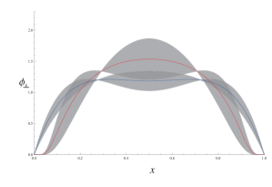
Figure 2: Twist-2 DAs predicted by hQCD (red curve) and SR (blue curve). The uncertainty band is due to the variation of the quark mass and the fundamental scale for holographic QCD and the error bar on Gegenbauer coefficients for SR.

Figure 2 shows twist-2 DAs $\phi_{\parallel,\perp}(x,\;\mu=1\;{\rm GeV})$ for the $\phi$ vector meson obtained using Eqs. 19 and 20 as compared to SR predictions as given by Eq. 23. The uncertainty band for holographic DAs are due to the uncertainties in quark mass and the fundamental AdS/QCD scale: $m_{s}=0.40\pm 0.15$ GeV and $\kappa=0.54\pm 0.02$ GeV. The error band in SR DAs are the result of the uncertainties in the Gegenbauer coefficients as given above.

The twist-3 DAs can also be obtained from the light-front wavefunction through the following expressions Ahmady and Sandapen (2013a)

$$g_{\perp}^{(v)}(x)=\frac{N_{c}}{2\pi f_{\phi}m_{\phi}}\int{\mathrm{d}}b\mu J_{1}(\mu b)[m_{s}^{2}-(x^{2}+(1-x)^{2}\nabla_{b}^{2})]\frac{\Psi^{\phi}_{T}(x,\zeta)}{x^{2}(1-x)^{2}}\;,$$ (24)

$$\frac{{\mathrm{d}}g_{\perp}^{(a)}(x)}{{\mathrm{d}}x}=\frac{\sqrt{2}N_{c}}{\pi f_{\phi}m_{\phi}}\int{\mathrm{d}}b\mu J_{1}(\mu b)[(1-2x)m_{s}^{2}-\nabla_{b}^{2})]\frac{\Psi^{\phi}_{T}(x,\zeta)}{x^{2}(1-x)^{2}}\;,$$ (25)

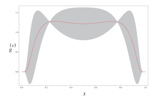
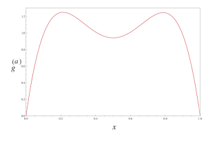
Figure 3: Twist-3 DAs $g^{(v)}$ and $g^{(a)}$ predicted by hQCD. The uncertainty band is due to the variation of the quark mass and the fundamental scale for holographic QCD.

Figure 3 shows the twist-3 DAs for $\phi$ meson which are obtained from Eqns 24 and 25. As is evident from the figures, the uncertainty due to $m_{s}$ and $\kappa$, contrary to the case for $g^{(v)}$, is negligible for $g^{(a)}$. In the next section, we use the decay constants and DAs up to twist-3 to compute the transition form factors (TFFs) $B_{s}\to\phi$.

V $B_{s}\rightarrow\phi$ transition form factors

The seven $B_{s}\to\phi$ TTFs are defined asHorgan et al. (2014)

$$\langle\phi(k,\varepsilon)|\bar{s}\gamma^{\mu}(1-\gamma^{5})b|B_{s}(p)\rangle = \frac{2iV(q^{2})}{m_{B_{s}}+m_{\phi}}\epsilon^{\mu\nu\rho\sigma}\varepsilon^{*}_{\nu}k_{\rho}p_{\sigma}-2m_{\phi}A_{0}(q^{2})\frac{\varepsilon^{*}\cdot q}{q^{2}}q^{\mu}$$ (26)

$$- (m_{B_{s}}+m_{\phi})A_{1}(q^{2})\left(\varepsilon^{\mu*}-\frac{\varepsilon^{*}\cdot qq^{\mu}}{q^{2}}\right)$$

$$+ A_{2}(q^{2})\frac{\varepsilon^{*}\cdot q}{m_{B_{s}}+m_{\phi}}\left[(p+k)^{\mu}-\frac{m_{B_{s}}^{2}-m_{\phi}^{2}}{q^{2}}q^{\mu}\right],$$

$$q_{\nu}\langle\phi(k,\varepsilon)|\bar{s}\sigma^{\mu\nu}(1+\gamma^{5})b|B_{s}(p)\rangle = 2T_{1}(q^{2})\epsilon^{\mu\nu\rho\sigma}\varepsilon^{*}_{\nu}p_{\rho}k_{\sigma}$$ (27)

$$+ iT_{2}(q^{2})[(\varepsilon^{*}\cdot q)(p+k)_{\mu}-\varepsilon_{\mu}^{*}(m_{B_{s}}^{2}-m_{\phi}^{2})]$$

$$+ iT_{3}(q^{2})(\varepsilon^{*}\cdot q)\left[\frac{q^{2}}{m_{B_{s}}^{2}-m_{\phi}^{2}}(p+k)_{\mu}-q_{\mu}\right],$$

where $q=p-k$ is the 4-momentum transfer and $\epsilon$ is the polarization 4-vector of the $\phi$. At low-to-intermediate values of $q^{2}$, these TFFs can be computed using QCD light-cone sum rules (LCSR) Ali et al. (1994); Aliev et al. (1997); Ball and Zwicky (2005). Here we use the LCSR expressions from Ref.Ahmady et al. (2014b) which are modified for the $B_{s}\to\phi$ decay channel. Table 2 shows the numerical values of the input parameters used in our predictions of the TFFs and the decay rate.

$m_{B_{s}}$	$5.367\;\mathrm{GeV}$	$M_{B}$	$8\;\mathrm{GeV}^{2}$
$\alpha^{-1}$	$127$	$s_{0}$	$36\;\mathrm{GeV}^{2}$
$|V_{tb}V_{ts}^{*}|$	$0.0407$	$f_{B_{s}}$	$0.224\;\mathrm{GeV}$
$\tau_{B_{s}}$	$1.512\;\mathrm{ps}$	$m_{b}$	$4.8\;\mathrm{GeV}$

Table 2: Numerical values of the input parameters.

The form factors, computed via LCSR, are valid at low to intermediate $q^{2}$. The extrapolation to high $q^{2}$ is performed via a two-parameter fit of the following form

$$F(q^{2})=\frac{F(0)}{1-a(q^{2}/m_{B_{s}}^{2})+b(q^{4}/m_{B_{s}}^{4})}$$ (28)

to the LCSR predictions as well as form factor values obtained by lattice QCD which are available at high $q^{2}$. The results for the above fit are given in Table 3. We note that hQCD predicts lower values of the form factors at $q^{2}=0$ compared to those obtained from SR.

	V	$A_{0}$	$A_{1}$	$A_{2}$	$T_{1}$	$T_{2}$	$T_{3}$
F(0) (hQCD)	$0.26\pm 0.2$	$0.15\pm 0.03$	$0.19\pm 0.02$	$0.21\pm 0.01$	$0.21\pm 0.03$	$0.22\pm 0.01$	$0.16\pm 0.01$
F(0) (SR)	$0.33\pm 0.01$	$0.27\pm 0.01$	$0.26\pm 0.01$	$0.26\pm 0.01$	$0.27\pm 0.01$	$0.28\pm 0.01$	$0.18\pm 0.01$
a (hQCD)	$1.66\pm 0.06$	$2.21^{+0.18}_{-0.15}$	$0.85^{+0.08}_{-0.07}$	$1.41\pm 0.22$	$1.76^{+0.20}_{-0.16}$	$0.51\pm 0.01$	$0.55^{+0.32}_{-0.42}$
a (SR)	$1.50\pm 0.01$	$1.26\pm 0.03$	$0.24\pm 0.02$	$1.35^{+0.31}_{-0.12}$	$1.51\pm 0.02$	$0.046\pm 0.01$	$0.73\pm 0.19$
b (hQCD)	$0.60^{+0.08}_{-0.07}$	$1.26^{+0.24}_{-0.19}$	$-0.23^{+0.07}_{-0.06}$	$0.51^{+0.66}_{-0.13}$	$0.74^{+0.25}_{-0.20}$	$-0.63\pm 0.05$	$-0.98^{+0.44}_{-0.55}$
b (SR)	$0.45\pm 0.01$	$-0.013\pm 0.048$	$-0.86\pm 0.03$	$0.62^{+0.85}_{-0.39}$	$0.48\pm 0.03$	$-1.08\pm 0.03$	$-0.65^{+0.23}_{-0.19}$

Table 3: hQCD+ lattice predictions for the form factors. Lattice data are taken from Horgan et al. (2014). The error bars for the holographic form factors are due to the variation in $m_{s}$ and $\kappa$, as explained in the text.

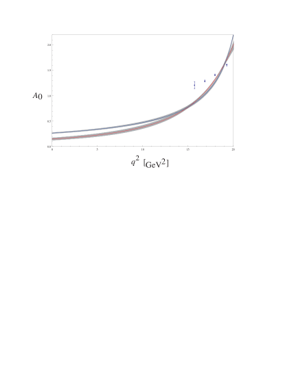
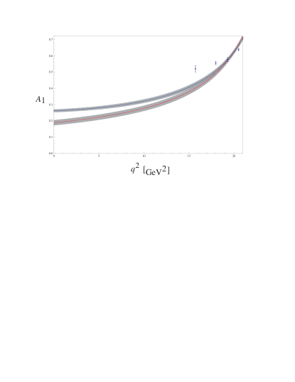
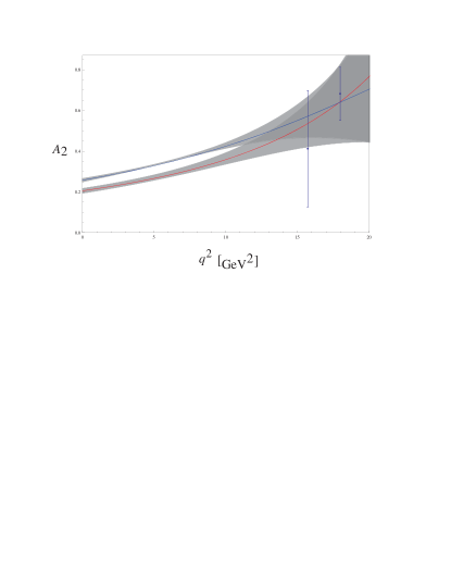
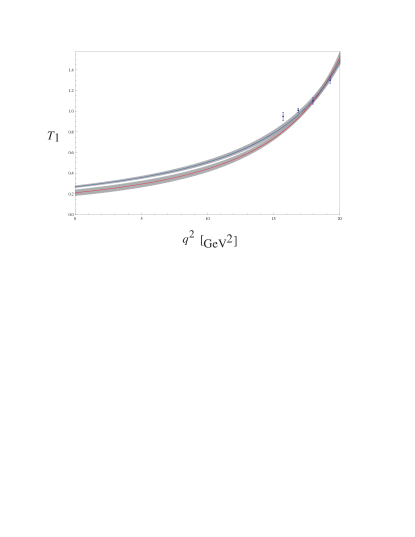
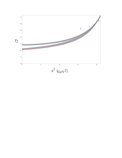
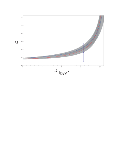
Figure 4: hQCD (red curves) and QCDSR (blue curves) predictions for the $B_{s}\to\phi$ TFFs. The two-parameter fits with the available lattice data are used for the plots. The shaded bands represent the uncertainty in the predicted form factors due to uncertainty bands in DAs and variation in quark masses. Lattice data points (shown on plots) are taken from Horgan et al. (2014).

Figure 4 shows the comparison between hQCD and SR predictions including the lattice data points at high $q^{2}$ for the form factors. The shaded bands in these figures represent the uncertainty due to the error band in the DAs. Note that there are additional uncertainties in the form factors inherent in the LCSR method (uncertainty in the Borel parameter, continuum threshold and other input parameters). Since our goal in this paper is to discriminate between the hQCD and SR models and that the inherent LCSR uncertainties are the same in both models, we do not include them here.

VI Differential decay rate

The differential branching ratio for $B_{s}\to\phi\mu^{+}\mu^{-}$ is given by the following expression Aliev et al. (1997):

$$\frac{d\mathcal{B}}{dq^{2}}=\tau_{B_{s}}\frac{G_{F}^{2}\alpha^{2}}{2^{11}\pi^{5}}\frac{|{V_{tb}V_{ts}^{*}|^{2}\sqrt{\lambda}v}}{3m_{B_{s}}}((2m_{\mu}^{2}+m_{B_{s}}^{2}s)[16(|A|^{2}+|C|^{2})m_{B_{s}}^{4}\lambda+2(|B_{1}|^{2}+|D_{1}|^{2})$$

$$\times\frac{\lambda+12rs}{rs}+2(|B_{2}|^{2}+|D_{2}|^{2})\frac{m_{B_{s}}^{4}\lambda^{2}}{rs}-4[\Re\mbox{e}(B_{1}B_{2}^{*})+\Re\mbox{e}(D_{1}D_{2}^{*})]\frac{m_{B_{s}}^{2}\lambda}{rs}(1-r-s)]$$

$$+6m_{\mu}^{2}[-16|C|^{2}m_{B_{s}}^{4}\lambda+4\Re\mbox{e}(D_{1}D_{3}^{*})\frac{m_{B_{s}}^{2}\lambda}{r}-4\Re\mbox{e}(D_{2}D_{3}^{*})\frac{m_{B_{s}}^{4}(1-r)\lambda}{r}+2|D_{3}|^{2}\frac{m_{B_{s}}^{4}s\lambda}{r}$$

$$-4\Re\mbox{e}(D_{1}D_{2}^{*})\frac{m_{B_{s}}^{2}\lambda}{r}-24|D_{1}|^{2}+2|D_{2}|^{2}\frac{m_{B_{s}}^{4}\lambda}{r}(2+2r-s)])$$

where $\lambda=1+r^{2}+s^{2}-2r-2s-2rs$, with $r=m_{\phi}^{2}/m_{B_{s}}^{2}$ and $s=q^{2}/m_{B_{s}}^{2}$. The final muon has mass $m_{\mu}$ and velocity $v=\sqrt{1-4m_{\mu}^{2}/q^{2}}$. The differential branching fraction depends on the following combinations of form factors:

$$A=C_{9}^{eff}\left(\frac{V}{m_{B_{s}}+m_{\phi}}\right)+4C_{7}\frac{m_{b}}{q^{2}}T_{1}\;,$$ (29)

$$B_{1}=C_{9}^{eff}(m_{B_{s}}+m_{\phi})A_{1}+4C_{7}\frac{m_{b}}{q^{2}}(m_{B_{s}}^{2}-m_{\phi}^{2})T_{2}\;,$$ (30)

$$B_{2}=C_{9}^{eff}\left(\frac{A_{2}}{m_{B_{s}}+m_{\phi}}\right)+4C_{7}\frac{m_{b}}{q^{2}}\left(T_{2}+\frac{q^{2}}{m_{B_{s}}^{2}-m_{\phi}^{2}}T_{3}\right)\;,$$ (31)

$$C=C_{10}\left(\frac{V}{m_{B_{s}}+m_{\phi}}\right)\;,$$ (32)

$$D_{1}=C_{10}(m_{B_{s}}+m_{\phi})A_{1}\;,$$ (33)

$$D_{2}=C_{10}\left(\frac{A_{2}}{m_{B_{s}}+m_{\phi}}\right)\;,$$ (34)

and

$$D_{3}=-C_{10}\frac{2m_{\phi}}{q^{2}}\left(A_{3}-A_{0}\right)\;,$$ (35)

where

$$A_{3}=A_{0}-\frac{q^{2}}{2m_{\phi}}\frac{A_{2}}{m_{B_{s}}+m_{\phi}}\;.$$ (36)

As for the SM Wilson coefficients $C_{7}$, $C_{9}^{eff}=C_{9}+Y(q^{2})$ and $C_{10}$ appearing in the above equations, are given in Ref. Altmannshofer et al. (2009) . Figure 5 shows the hQCD and QCDSR predictions for $B_{s}\to\phi\mu^{+}\mu^{-}$ differential branching ratio compared with the available experimental data from LHCb Aaij et al. (2015). We observe that at low momentum transfer where the form factors are most sensitive to DAs through LCSR, hQCD produces better agreement with the data. The bin-by-bin numerical predictions are given in Table 4.

Using our hQCD predictions for $B\to K^{*}\mu^{+}\mu^{-}$ decay Ahmady et al. (2015), we can consider the ratio

$$R_{K^{*}\phi}[q_{1},\;q_{2}]=\frac{dBR(B^{0}\to K^{*0}\mu^{+}\mu^{-})/dq^{2}|_{[q_{1},\;q_{2}]}}{dBR(B_{s}\to\phi\mu^{+}\mu^{-})/dq^{2}|_{[q_{1},\;q_{2}]}}\;,$$ (37)

by using the differential branching ratios integrated over range $[q_{1},\;q_{2}]$. Figure 6 shows a graphical comparison of our predictions for $R_{K^{*}\phi}$ to the experimental data of LHCb Aaij et al. (2013b, 2014a) and CDF Cdf (2012) at low and high $q^{2}$ range. It is encouraging that in low $q^{2}$, the hQCD prediction agrees, within the error bars, with both LHCb and CDF results. Again, one should note that LCSR method for the evaluation of the transition form factors are expected to be more reliable at low $q^{2}$. On the other hand, at high $q^{2}$, our prediction only agrees with the CDF datum.

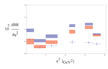
Figure 5: The differential branching ratio for $B_{s}\to\phi\mu^{+}\mu^{-}$ as predicted by hQCD (red rectangles) and SR (blue rectangles). The uncertainty widths are due to the form factors. The experimental data points are measured by LHCb Aaij et al. (2015).

$q^{2}$ (GeV)	$10^{7}\langle\mathcal{BR}^{hQCD}\rangle$	$10^{7}\langle\mathcal{BR}^{QCDSR}\rangle$	$10^{7}\langle\mathcal{BR}^{experiment}\rangle$
$0.1-2.0$	$0.49^{+0.12}_{-0.11}$	$0.96{\pm}0.07$	$0.59\pm 0.07$
$2-5$	$0.29^{+0.05}_{-0.07}$	$0.54^{+0.05}_{-0.07}$	$0.26\pm 0.04$
$5-8$	$0.48^{+0.06}_{-0.08}$	$0.73^{+0.06}_{-0.09}$	$0.32\pm 0.04$
$11.0-12.5$	$0.91^{+0.07}_{-0.08}$	$1.15{\pm}0.06$	$0.47\pm{0.07}$
$15-17$	$1.08^{+0.07}_{-0.06}$	$1.21\pm 0.05$	$0.45^{+0.06}_{-0.05}$
$17.0-19.0$	$0.75\pm 0.04$	$0.80^{+0.04}_{-0.03}$	$0.40_{-0.05}^{+0.06}$

Table 4: Bin-by-bin hQCD and QCDSR predictions for the $B_{s}\to\phi\mu^{+}\mu^{-}$ branching ratio compared with the experimental data from LHCb Aaij et al. (2015).

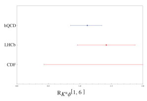
Figure 6: hQCD prediction for $R_{K^{*}\phi}$ at low and hight $q^{2}$ ranges as compared with the experimental data from LHCb Aaij et al. (2013b, 2014a) and CDFCdf (2012).

VII Conclusion

We have calculated the $B_{s}\to\phi$ transition form factors using $\phi$ meson holographic DAs. Our prediction for the $B_{s}\to\phi\mu^{+}\mu^{-}$ differential branching ratio is in better agreement with the latest LHCb data than the prediction generated using QCDSR DAs. In addition, we found that the hQCD prediction for $R_{K^{*}\phi}$ is in excellent agreement with both LHCb and CDF data at low $q^{2}$. We conclude that it is important to have a better understanding of non-perturbative effects in rare $B_{(s)}$ decays.

VIII Acknowledgments

M. A and R. S are supported by Individual Discovery Grants from the Natural Science and Engineering Research Council of Canada (NSERC): SAPIN-2017-00033 and SAPIN-2017-00031 respectively. We would like to thank Idriss Amadou Ali for his contribution in the numerical computations of this work.

References

- Aaltonen et al. (2011a) T. Aaltonen et al. (CDF), Phys. Rev. Lett. 106, 161801 (2011a), eprint 1101.1028.
- Aaltonen et al. (2011b) T. Aaltonen et al. (CDF), Phys. Rev. Lett. 107, 201802 (2011b), eprint 1107.3753.
- Aaij et al. (2013a) R. Aaij et al. (LHCb), JHEP 07, 084 (2013a), eprint 1305.2168.
- Altmannshofer and Straub (2015) W. Altmannshofer and D. M. Straub, Eur. Phys. J. C75, 382 (2015), eprint 1411.3161.
- Aaij et al. (2015) R. Aaij et al. (LHCb), JHEP 09, 179 (2015), eprint 1506.08777.
- Bharucha et al. (2016) A. Bharucha, D. M. Straub, and R. Zwicky, JHEP 08, 098 (2016), eprint 1503.05534.
- Geng and Liu (2003) C. Q. Geng and C. C. Liu, J. Phys. G29, 1103 (2003), eprint hep-ph/0303246.
- Aaij et al. (2013b) R. Aaij et al. (LHCb), JHEP 08, 131 (2013b), eprint 1304.6325.
- Aaij et al. (2014a) R. Aaij et al. (LHCb), JHEP 06, 133 (2014a), eprint 1403.8044.
- Aaij et al. (2014b) R. Aaij et al. (LHCb), JHEP 10, 064 (2014b), eprint 1408.1137.
- Ali et al. (1994) A. Ali, V. M. Braun, and H. Simma, Z. Phys. C63, 437 (1994), eprint hep-ph/9401277.
- Ahmady et al. (2016) M. Ahmady, R. Sandapen, and N. Sharma, Phys. Rev. D94, 074018 (2016), eprint 1605.07665.
- de Teramond and Brodsky (2005) G. F. de Teramond and S. J. Brodsky, Phys. Rev. Lett. 94, 201601 (2005), eprint hep-th/0501022.
- Brodsky and de Teramond (2006) S. J. Brodsky and G. F. de Teramond, Phys. Rev. Lett. 96, 201601 (2006), eprint hep-ph/0602252.
- de Teramond and Brodsky (2009) G. F. de Teramond and S. J. Brodsky, Phys. Rev. Lett. 102, 081601 (2009), eprint 0809.4899.
- Brodsky et al. (2015) S. J. Brodsky, G. F. de Teramond, H. G. Dosch, and J. Erlich, Phys. Rept. 584, 1 (2015), eprint 1407.8131.
- de Alfaro et al. (1976) V. de Alfaro, S. Fubini, and G. Furlan, Nuovo Cim. A34, 569 (1976).
- Brodsky et al. (2013) S. J. Brodsky, G. F. de Téramond, and H. G. Dosch, Nuovo Cim. C036, 265 (2013), eprint 1302.5399.
- Brodsky and de Teramond (2009) S. J. Brodsky and G. F. de Teramond, Subnucl. Ser. 45, 139 (2009), eprint 0802.0514.
- Forshaw and Sandapen (2012) J. R. Forshaw and R. Sandapen, Phys. Rev. Lett. 109, 081601 (2012), eprint 1203.6088.
- Ahmady et al. (2018) M. Ahmady, A. Leger, Z. Mcintyre, A. Morrison, and R. Sandapen, Phys. Rev. D98, 053002 (2018), eprint 1805.02940.
- Ahmady et al. (2015) M. Ahmady, D. Hatfield, S. Lord, and R. Sandapen, Phys. Rev. D92, 114028 (2015), eprint 1508.02327.
- Ahmady et al. (2014a) M. R. Ahmady, S. Lord, and R. Sandapen, Phys. Rev. D90, 074010 (2014a), eprint 1407.6700.
- Ahmady et al. (2014b) M. Ahmady, R. Campbell, S. Lord, and R. Sandapen, Phys. Rev. D89, 074021 (2014b), eprint 1401.6707.
- Ahmady and Sandapen (2013a) M. Ahmady and R. Sandapen, Phys. Rev. D88, 014042 (2013a), eprint 1305.1479.
- Ahmady and Sandapen (2013b) M. Ahmady and R. Sandapen, Phys. Rev. D87, 054013 (2013b), eprint 1212.4074.
- Ball et al. (1998) P. Ball, V. M. Braun, Y. Koike, and K. Tanaka, Nucl. Phys. B529, 323 (1998), eprint hep-ph/9802299.
- Tanabashi et al. (2018) M. Tanabashi et al. (Particle Data Group), Phys. Rev. D98, 030001 (2018).
- Anastasi et al. (2017) A. Anastasi et al. (KLOE-2), Phys. Lett. B767, 485 (2017), eprint 1609.06631.
- Ball and Braun (1998) P. Ball and V. M. Braun, Phys. Rev. D58, 094016 (1998), eprint hep-ph/9805422.
- Becirevic et al. (2003) D. Becirevic, V. Lubicz, F. Mescia, and C. Tarantino, JHEP 05, 007 (2003), eprint hep-lat/0301020.
- Braun et al. (2003) V. M. Braun, T. Burch, C. Gattringer, M. Gockeler, G. Lacagnina, S. Schaefer, and A. Schafer, Phys. Rev. D68, 054501 (2003), eprint hep-lat/0306006.
- Jansen et al. (2009) K. Jansen, C. McNeile, C. Michael, and C. Urbach (ETM), Phys. Rev. D80, 054510 (2009), eprint 0906.4720.
- Gao et al. (2014) F. Gao, L. Chang, Y.-X. Liu, C. D. Roberts, and S. M. Schmidt, Phys. Rev. D90, 014011 (2014), eprint 1405.0289.
- Ball et al. (2007) P. Ball, V. M. Braun, and A. Lenz, JHEP 08, 090 (2007), eprint 0707.1201.
- Choi and Ji (2007) H.-M. Choi and C.-R. Ji, Phys. Rev. D75, 034019 (2007), eprint hep-ph/0701177.
- Ball and Jones (2007) P. Ball and G. W. Jones, Journal of High Energy Physics 2007, 069 (2007), URL https://doi.org/10.1088%2F1126-6708%2F2007%2F03%2F069.
- Horgan et al. (2014) R. R. Horgan, Z. Liu, S. Meinel, and M. Wingate, Phys. Rev. D89, 094501 (2014), eprint 1310.3722.
- Aliev et al. (1997) T. M. Aliev, A. Ozpineci, and M. Savci, Phys. Rev. D56, 4260 (1997), eprint hep-ph/9612480.
- Ball and Zwicky (2005) P. Ball and R. Zwicky, Phys. Rev. D71, 014029 (2005), eprint hep-ph/0412079.
- Altmannshofer et al. (2009) W. Altmannshofer, P. Ball, A. Bharucha, A. J. Buras, D. M. Straub, and M. Wick, JHEP 01, 019 (2009), eprint 0811.1214.
- Cdf (2012) CDF Public Note 10894 (2012).