Quantum ion thermodynamics in liquid interiors of white dwarfs

Abstract

We present an accurate analytic approximation for the energy of a quantum one-component Coulomb liquid of ions in a uniform electron background which has been recently calculated from first principles (Baiko 2019). The approximation enables us to develop in an analytic form a complete thermodynamic description of quantum ions in a practically important range of mass densities at temperatures above crystallization. We show that ionic quantum effects in liquid cores of white dwarfs (WDs) affect heat capacity, cooling, thermal compressibility, pulsation frequencies and radii of sufficiently cold WDs, especially with relatively massive helium and carbon cores.

1 Introduction

Thanks to Sloan Digital Sky Survey, Gaia and other projects, current progress in highly precise observations and theoretical interpretation of WDs is fantastically rapid (e.g., Genest-Beaulieu & Bergeron 2019; Bergeron et al. 2019; Kepler et al. 2019; Pelisoli & Vos 2019). For instance, we can mention studies of cooling WDs (e.g., Tremblay et al. 2019; Fernandes et al. 2019; Blouin et al. 2019) and asteroseismology (e.g., Córsico et al. 2019; Bischoff-Kim et al. 2019). The rapid observational progress motivates further theoretical studies of dense matter in WD interiors.

Recently, Baiko (2019) (hereafter Paper I) has calculated from first principles the energy of a liquid quantum one-component plasma (OCP) of ions immersed in a uniform charge-compensating background of electrons. This is a suitable model to describe dense plasma of ions in degenerate cores of WDs. The author presented his results in a tabular form and illustrated them by calculating temperature dependence of the ion specific heat at two combinations of density and composition (using an interpolation of the tabulated data). Also, he pointed out a number of applications of these results for WDs (as well as for the envelopes of neutron stars).

In Section 2, we present an analytic fit to the results of Paper I. It allows us to construct thermodynamics of a quantum one-component ion liquid in a closed form thereby facilitating usage of the results of Paper I in applications. In Section 3, we employ these fitting formulae to study quantitatively the ionic quantum effects in liquid cores of WDs and assess their importance. We conclude in Section 4.

2 Analytic formulation

2.1 Ion plasma parameters

Thermodynamic state of the OCP of ions immersed in a rigid electron background can be characterized by two dimensionless parameters (e.g., Haensel et al. 2007),

$$\Gamma=\frac{Z_{i}^{2}e^{2}}{k_{\rm B}Ta},\quad\eta=\frac{T_{\rm p}}{T\sqrt{3}}.$$ (1)

Here, $Z_{i}$ is the ion charge number, $e$ is the elementary charge, and $k_{\rm B}$ is the Boltzmann constant. Furthermore, $T$ is the temperature, $a=(4\pi n_{i}/3)^{-1/3}$ is the ion-sphere radius determined by the number density of ions $n_{i}$; $T_{\rm p}=(\hbar/k_{\rm B})\sqrt{4\pi n_{i}Z_{i}^{2}e^{2}/M_{i}}$ is the ion plasma temperature and $M_{i}$ is the ion mass.

The first quantity, the Coulomb-coupling parameter $\Gamma$, measures the ratio of the typical potential and kinetic energies of ions. If $\Gamma\ll 1$, the ions are weakly coupled (constitute Boltzmann gas). In the opposite limit of $\Gamma\gg 1$, they form a strongly coupled Coulomb plasma, liquid or solid. If one disregards quantum effects in ion motion, melting occurs at $\Gamma=\Gamma_{\rm m}\approx 175$ (Potekhin & Chabrier, 2000). The melting temperature is

$$T_{\rm m}=\frac{Z_{i}^{2}e^{2}}{k_{\rm B}a\Gamma_{\rm m}}.$$ (2)

The second parameter $\eta$ in equation (1) characterizes the strength of the ion quantum effects. These effects are known to be especially important for sufficiently light ions at relatively low temperatures and/or high densities ($\eta\gtrsim 1$). In a quantum system, one has $T\ll T_{\rm p}$. Another familiar quantum-mechanical parameter is $r_{\rm s}=a/a_{0}$, where $a_{0}=\hbar^{2}/(M_{i}Z_{i}^{2}e^{2})$ is the ionic Bohr radius. These quantities are related as

$$\eta=\frac{\Gamma}{\sqrt{r_{\rm s}}}~{}.$$ (3)

2.2 Analytic fit

Energy $E_{i}$ of a quantum Coulomb plasma of ions with uniform incompressible electron background was calculated in Paper I (table 1) neglecting ion exchange effects on a dense grid of values of $\Gamma$ ($1\leq\Gamma\leq 175$, 25 grid points) and $r_{s}$ ($600\leq r_{s}\leq 12000$, 15 points; 25$\times 15=375$ grid points in total). Here, these results are approximated by the following analytic expression,

$$\frac{E_{i}-E_{0}}{N_{i}k_{\rm B}T}=\frac{3}{2}-\zeta\Gamma+u_{\rm cl}(\Gamma)+u_{\rm q}(\eta)~{}.$$ (4)

The functions which enter equation (4) are described below and the fit parameters are given in Table 1. The relative root mean square error of the fit over all grid points is $0.0014$ while the maximum relative error of 0.0043 takes place at $\Gamma=73.5$ and $r_{s}=4800$. Such fit accuracy seems acceptable for astrophysical applications. An explicit formula is much easier to use than tabulated values; it allows one to differentiate and integrate analytically over temperature and density for constructing various thermodynamic quantities of the ion plasma.

The quantity on the left-hand side of equation (4) was calculated and tabulated in Paper I [where it was denoted as $(E-E_{0})/(NT)$ whereas $k_{\rm B}$ was set equal to 1], $E_{0}=\zeta\Gamma N_{i}k_{\rm B}T$ is the electrostatic (Madelung) energy of an ideal body centered cubic (bcc) Coulomb crystal ($\zeta\approx-0.895929255682$), and $N_{i}$ is the number of ions. Furthermore, $u_{\rm cl}(\Gamma)$ represents the fit proposed by Potekhin & Chabrier (2000) for their ‘ion-ion’ component of the energy of a classic Coulomb plasma,

$$u_{\rm cl}(\Gamma)=\Gamma^{3/2}\left[\frac{A_{1}}{\sqrt{A_{2}+\Gamma}}+\frac{A_{3}}{1+\Gamma}\right]+\frac{B_{1}\Gamma^{2}}{B_{2}+\Gamma}+\frac{B_{3}\Gamma^{2}}{B_{4}+\Gamma^{2}}~{},$$ (5)

with $A_{3}=-\sqrt{3}/2-A_{1}/\sqrt{A_{2}}$. At $\Gamma>1$, the fit (4) without the last term $u_{\rm q}$ reproduces Monte Carlo (MC) results of Dewitt & Slattery (1999) while at $\Gamma<1$, it interpolates between these MC results and a well known exact analytic expression. In the latter case quantum corrections become insignificant; accordingly, equation (4) can be used at arbitrarily small $\Gamma$.

The quantum contribution to the energy is described by the last term of equation (4),

$$u_{\rm q}(\eta)=\frac{Q_{1}\eta^{2}}{Q_{2}+\eta}+\frac{Q_{3}\eta^{2}}{Q_{4}+\eta^{2}}~{}.$$ (6)

It turns out to be a function of a single parameter $\eta=T_{\rm p}/(\sqrt{3}T)$ given by equation (3). This fact seems nontrivial; it has not been expected from the beginning but the fit procedure indicates that it is so (at least within the fit accuracy). In the limit $\eta\to 0$, the quantum term is forced to reduce to the exact first-order Wigner-Kirkwood correction (e.g., Landau & Lifshitz 1980). This translates to the condition $Q_{1}/Q_{2}+Q_{3}/Q_{4}=1/4$ which allows one to calculate $Q_{3}$ through other coefficients $Q$ given in Table 1.

In the quantum limit of large $\eta$ (sufficiently small $r_{s}$), $u_{\rm q}\approx Q_{1}\eta$ which corresponds to a temperature-independent contribution to $E_{i}$. Such a term strongly resembles the zero-point energy of a harmonic Coulomb solid which has the same temperature and density dependence but a different coefficient. In the liquid, the term in question is $(Q_{1}/\sqrt{3})N_{i}k_{\rm B}T_{\rm p}\approx 3.46N_{i}k_{\rm B}T_{\rm p}$ whereas in the harmonic Coulomb solid $E_{\rm zero-point}=(3/2)u_{1}N_{i}k_{\rm B}T_{\rm p}\approx 0.767N_{i}k_{\rm B}T_{\rm p}$ where we have set $u_{1}\approx 0.5114$ which is the first bcc phonon spectral moment (e.g., Baiko et al. 2001). We see that the coefficient in the liquid is 4.5 times larger than that in the bcc solid.

Table 1: Fit coefficients in equation (4) ^a)

$A_{1}$	$A_{2}$	$B_{1}$	$B_{2}$	$B_{3}$	$B_{4}$	$Q_{1}$	$Q_{2}$	$Q_{4}$
$-$0.9070	0.62954	0.00456	211.6	$-$0.0001	0.00462	5.994	70.3	22.7

^a) Coefficients $A$ and $B$ are taken from Potekhin & Chabrier (2000); only coefficients $Q$ have been varied to fit the data (see text for details).

Formally, the fit (4) is based on the data at $\Gamma\leq\Gamma_{\rm m}$ ($T\geq T_{\rm m}$), that is at temperatures higher than the melting temperature of a classic Coulomb liquid of ions. However, bearing in mind a sufficiently smooth dependence of $E_{i}$ on $T$ and $n_{i}$ we hope that we can extrapolate the fit to somewhat lower $T$ (larger $\Gamma$) to describe a supercooled Coulomb liquid or, actually, the ordinary quantum Coulomb liquid which in reality, due to quantum effects, solidifies at $\Gamma_{\rm m}$ slightly above the classic value of 175.

2.3 Constructing thermodynamics

Using the fit (4) we can construct analytic thermodynamics of quantum OCP of ions.

Multiplying equation (4) by $T$ and differentiating with respect to $T$ one obtains ionic isochoric heat capacity,

$$\frac{C_{Vi}}{k_{\rm B}N_{i}}\equiv\frac{{\cal C}_{Vi}}{k_{\rm B}n_{i}}=\frac{3}{2}+u_{\rm cl}(\Gamma)+u_{\rm q}(\eta)-\Gamma\frac{{\rm d}u_{\rm cl}}{{\rm d}\Gamma}-\eta\frac{{\rm d}u_{\rm q}}{{\rm d}\eta}~{},$$ (7)

where ${\cal C}_{Vi}$ is the heat capacity per unit volume. The Helmholtz free energy can be obtained by integration

$$\frac{F_{i}}{N_{i}k_{\rm B}T}=\frac{F_{\rm id}}{N_{i}k_{\rm B}T}+\int_{0}^{\Gamma}{\rm d}\Gamma^{\prime}\frac{u_{\rm cl}(\Gamma^{\prime})}{\Gamma^{\prime}}+\int_{0}^{\eta}{\rm d}\eta^{\prime}\frac{u_{\rm q}(\eta^{\prime})}{\eta^{\prime}}~{},$$ (8)

where $F_{\rm id}$ is the Helmholtz free energy of an ideal Boltzmann gas of ions. Then the ion pressure can be found as

$$P_{i}=-\left(\frac{\partial F_{i}}{\partial V}\right)_{T}=P_{\rm id}\left(1+\frac{1}{3}u_{\rm cl}+\frac{1}{2}u_{\rm q}\right)~{},$$ (9)

where $P_{\rm id}=n_{i}k_{\rm B}T$ is the ideal gas pressure. Other practically important (see Section 3.2) quantities are the isochoric temperature derivative of pressure

$$\left(\frac{\partial P_{i}}{\partial T}\right)_{V}=n_{i}k_{\rm B}\left(1+\frac{1}{3}u_{\rm cl}+\frac{1}{2}u_{\rm q}-\frac{\Gamma}{3}\frac{{\rm d}u_{\rm cl}}{{\rm d}\Gamma}-\frac{\eta}{2}\frac{{\rm d}u_{\rm q}}{{\rm d}\eta}\right)$$ (10)

and the isothermal compressibility of ions

$$\left(\frac{\partial P_{i}}{\partial n_{i}}\right)_{T}=k_{\rm B}T\left(1+\frac{1}{3}u_{\rm cl}+\frac{1}{2}u_{\rm q}+\frac{\Gamma}{9}\frac{{\rm d}u_{\rm cl}}{{\rm d}\Gamma}+\frac{\eta}{4}\frac{{\rm d}u_{\rm q}}{{\rm d}\eta}\right).$$ (11)

Evaluating integrals and derivatives in equations (7) – (11) one obtains

$$\frac{F_{i}}{N_{i}k_{\rm B}T} = \frac{F_{\rm id}}{N_{i}k_{\rm B}T}+A_{1}\sqrt{\Gamma(A_{2}+\Gamma)}-A_{1}A_{2}\ln{\left(\sqrt{\frac{\Gamma}{A_{2}}}+\sqrt{1+\frac{\Gamma}{A_{2}}}\right)}$$ (12)

$$+ 2A_{3}\left(\sqrt{\Gamma}-\arctan{\sqrt{\Gamma}}\right)$$

$$+ B_{1}\Gamma-B_{1}B_{2}\ln{\left(1+\frac{\Gamma}{B_{2}}\right)}+\frac{B_{3}}{2}\ln{\left(1+\frac{\Gamma^{2}}{B_{4}}\right)}$$

$$+ Q_{1}\eta-Q_{1}Q_{2}\ln{\left(1+\frac{\eta}{Q_{2}}\right)}+\frac{Q_{3}}{2}\ln{\left(1+\frac{\eta^{2}}{Q_{4}}\right)}$$

[note a typo in equation (16) of Potekhin & Chabrier (2000) which should contain $\Gamma/B_{2}$ rather than $\Gamma/B_{1}$ in one of the logarithms]. Furthermore,

$$\frac{C_{Vi}}{k_{\rm B}N_{i}} = \frac{3}{2}+\frac{\Gamma^{3/2}}{2}\left[\frac{A_{3}(\Gamma-1)}{(1+\Gamma)^{2}}-\frac{A_{1}A_{2}}{(A_{2}+\Gamma)^{3/2}}\right]$$ (13)

$$+ \Gamma^{2}\left[\frac{B_{3}(\Gamma^{2}-B_{4})}{(B_{4}+\Gamma^{2})^{2}}-\frac{B_{1}B_{2}}{(B_{2}+\Gamma)^{2}}\right]$$

$$+ \eta^{2}\left[\frac{Q_{3}(\eta^{2}-Q_{4})}{(Q_{4}+\eta^{2})^{2}}-\frac{Q_{1}Q_{2}}{(Q_{2}+\eta)^{2}}\right]~{},$$

$$\frac{1}{k_{\rm B}n_{i}}\frac{\partial P_{i}}{\partial T} = 1+\frac{\Gamma^{3/2}}{6}\left[\frac{A_{3}(\Gamma-1)}{(1+\Gamma)^{2}}-\frac{A_{1}A_{2}}{(A_{2}+\Gamma)^{3/2}}\right]$$ (14)

$$+ \frac{\Gamma^{2}}{3}\left[\frac{B_{3}(\Gamma^{2}-B_{4})}{(B_{4}+\Gamma^{2})^{2}}-\frac{B_{1}B_{2}}{(B_{2}+\Gamma)^{2}}\right]$$

$$+ \frac{\eta^{2}}{2}\left[\frac{Q_{3}(\eta^{2}-Q_{4})}{(Q_{4}+\eta^{2})^{2}}-\frac{Q_{1}Q_{2}}{(Q_{2}+\eta)^{2}}\right]~{},$$

$$\frac{1}{k_{\rm B}T}\frac{\partial P_{i}}{\partial n_{i}} = 1+\frac{\Gamma^{3/2}}{18}\left[\frac{A_{1}(9A_{2}+8\Gamma)}{(A_{2}+\Gamma)^{3/2}}+\frac{A_{3}(9+7\Gamma)}{(1+\Gamma)^{2}}\right]$$ (15)

$$+ \frac{\Gamma^{2}}{9}\left[\frac{B_{1}(5B_{2}+4\Gamma)}{(B_{2}+\Gamma)^{2}}+\frac{B_{3}(5B_{4}+3\Gamma^{2})}{(B_{4}+\Gamma^{2})^{2}}\right]$$

$$+ u_{q}(\eta)-\frac{\eta^{3}}{4}\left[\frac{Q_{1}}{(Q_{2}+\eta)^{2}}+\frac{2Q_{3}\eta}{(Q_{4}+\eta^{2})^{2}}\right]~{}.$$

These fairly simple formulae give a complete first-principle description of the OCP thermodynamics at temperatures above the melting temperature neglecting ion statistics effects, which are expected to be very small under realistic conditions. For applications to real systems, one has to add thermodynamic quantities of the degenerate electron gas and contributions stemming from electron screening. The latter contributions are typically small and will be neglected here (e.g., Haensel et al. 2007).

3 Astrophysical implications

To illustrate astrophysical significance of new thermodynamics, let us describe accompanying modifications of physical properties of WD matter which can result in potentially observable effects. We will consider liquid cores of WDs where the electrons are strongly degenerate. The degeneracy makes the electron gas almost rigid and justifies the validity of the OCP model. By way of illustration, we consider a liquid of single species of fully ionized atomic nuclei. Actually, WD matter can contain a mix of different bare nuclei at high densities and ions in various ionization states at low densities but our present formalism does not allow us to study neither quantum effects in dense multispecies mixtures nor incompletely ionized plasma.

While analyzing WD cores we will assume that they are isothermal at a temperature $T$. This is a good approximation for not too hot WDs because of high thermal conductivity of degenerate electrons (e.g., Swarzschild 1958; Shapiro & Teukolsky 1983). When a WD cools, $T$ slowly decreases. For all realistic values of the internal temperature, the effective surface temperature $T_{\rm s}$ of a WD remains much lower than $T$ because of poor thermal conduction in its non-degenerate and mildly-degenerate outer envelope. The envelope is typically thin and low-massive; its thickness decreases with time.

Warm WDs have liquid cores, the main subject of our study. At a certain stage the core crystallyzes starting from the center. As the star cools, the crystallization front propagates to the stellar envelope.

3.1 Heat capacity of liquid WD cores

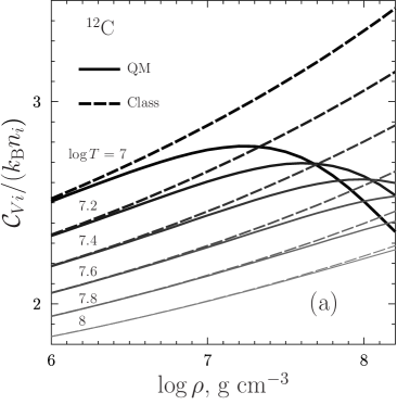
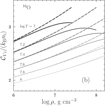
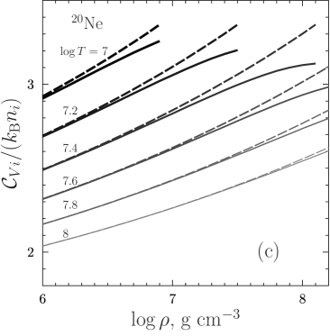
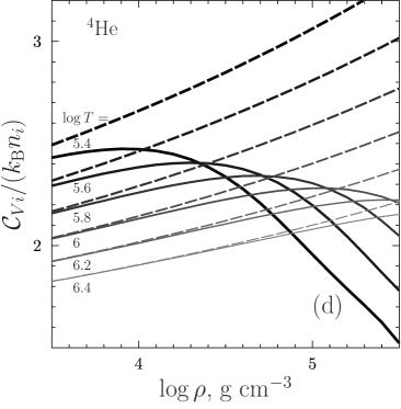
Figure 1: Ionic heat capacity per one ion (in units of $k_{\rm B}$) in a WD core composed of ¹²C (a), ¹⁶O (b), ²⁰Ne (c) and ⁴He (d) as a function of mass density for several temperatures above crystallization; values of $\log T$ (in K) are indicated near the curves. Solid (dashed) curves include (disregard) quantum effects of ions.

It is well known that ions in a WD core give the major contribution to the total heat capacity of the star.

In Fig. 1 we plot ionic heat capacity per one ion as a function of mass density $\rho$ for a range of internal WD temperatures $T$ above the melting temperature for four core compositions: ¹²C, ¹⁶O, ²⁰Ne and ⁴He [panels (a), (b), (c) and (d), respectively]. Some low-temperature curves for oxygen and neon are terminated at such densities where crystallization begins at a given $T$ ($T=T_{\rm m}$ for $\Gamma_{\rm m}=175$). Solid curves utilize full equation (13), including quantum effects, while dashed curves represent classic heat capacity, i.e. the first two lines of equation (13) only. As expected, quantum effects reduce the heat capacity; they are more pronounced for lighter elements, at higher densities and/or lower temperatures.

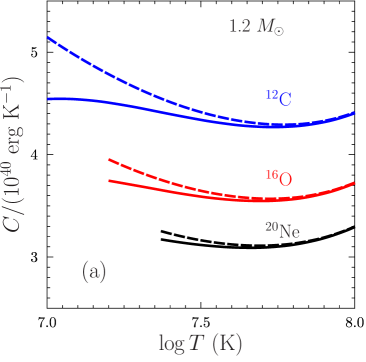
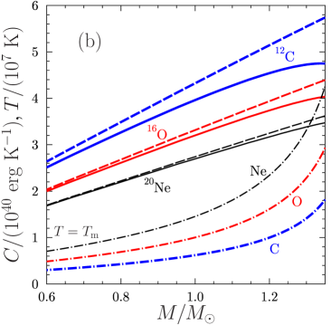
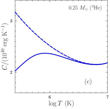
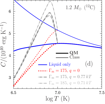
Figure 2: (a) Total heat capacity of a 1.2 M$\odot$ WD with isothermal liquid core of three compositions (marked near the curves) as a function of core temperature. Solid lines include and dashed lines exclude quantum effects of ions. (b) Total heat capacity of WDs with different core compositions as a function of WD mass. At each mass, the core temperature is equal to the melting temperature $T_{\rm m}$ in the WD center. Solid lines include and dashed lines exclude quantum effects. Three lower dash-dotted curves show respecive values of $T_{\rm m}$. (c) Same as in panel (a) but for a 0.25 M$\odot$ helium WD. (d) Effective heat capacity of a 1.2 M$\odot$ WD with isothermal carbon core as a function of core temperature with possible effects of crystallization and latent heat release (see text for details).

Fig. 2 presents the total heat capacity $C(T)$ of liquid isothermal cores of WDs of different masses, core compositions and internal temperatures,

$$C(T)=\int{\rm d}V\,{\cal C}(\rho,T),$$ (16)

where the integration is over the isothermal core, and ${\cal C}(\rho,T)$ is the heat capacity per unit volume; $C(T)$ is nearly equal to the total heat capacity of the star (contribution of the outer envelope is negligible). Even though the ionic contribution is typically dominant, we have also included the contribution of degenerate electrons, ${\cal C}={\cal C}_{Vi}+{\cal C}_{Ve}$. Because heat capacities of degenerate matter at constant volume and pressure are nearly the same (e.g., Haensel et al. 2007), we can safely add the ion and electron contributions at constant volume. The ion heat capacity per unit volume is calculated from equation (13) as ${\cal C}_{Vi}=(C_{Vi}/N_{i})n_{i}$. The electron contribution is calculated with the aid of the standard Sommerfeld expansion (e.g., Landau & Lifshitz, 1980),

$${\cal C}_{Ve}=\frac{k_{\rm B}^{2}{\rm\pi}^{2}Tn_{e}}{p_{{\rm F}e}v_{{\rm F}e}}~{},$$ (17)

where $n_{e}$ is the electron number density, while $p_{{\rm F}e}$ and $v_{{\rm F}e}$ are the electron Fermi momentum and velocity, respectively. The envelope-core boundary is set at a density where the electron degeneracy temperature is three times higher than $T$.

Since our figures are illustrative, our basic WD models are calculated using only the pressure of strongly degenerate electrons at $T=0$ (the only exception is Fig. 6). These models accurately reflect the main problem of WD study: at a given central density all WDs whose cores contain ions (⁴He, ¹²C, ¹⁶O or ²⁰Ne) with the same mass number to charge number ratio ($A_{i}/Z_{i}=2$) have nearly identical internal mass density distributions and nearly the same masses $M$ and radii $R$. This property complicates strongly the determination of the internal composition of WDs from observations and motivates studies of such observational manifestations which are sensitive to the internal composition.

Integrated heat capacities $C(T)$ are good to this aim. They do depend on internal composition of WDs and they are important for WD cooling theory (e.g., Swarzschild 1958; Shapiro & Teukolsky 1983). Because WD cooling is observable it can give valuable information on the internal composition.

Cooling of a WD with an isothermal core is governed by the equation

$$\frac{{\rm d}T}{{\rm d}t}=-\frac{L}{C(T)},$$ (18)

where $L$ is the total thermal energy loss rate of the star which is a sum of the thermal surface luminosity $L_{\rm s}=4\mathrm{\pi}\sigma R^{2}T_{\rm s}^{4}$ ($\sigma$ being the Stefan-Boltzmann constant) and the neutrino luminosity $L_{\nu}$ from the entire WD volume. The isothermal-core approximation is usually valid in not too warm WDs (not in pre-WDs) where neutrino cooling becomes inefficient and $L\approx L_{\rm s}$.

In Fig. 2(a), we plot the integrated heat capacity of a 1.2 M$\odot$ ($R\approx 4180$ km) WD with a carbon, oxygen or neon core (blue, red or black curves, respectively) as a function of the core temperature (above melting). Solid (dashed) curves include (exclude) ion quantum effects. Once again one observes an amplification of the quantum effects with decreasing temperature and atomic number of ions. A general decreasing trend of the heat capacity with increase of the atomic number is simply because $C(T)$ is proportional to the number of ions, and there is fewer heavier ions in a star of a fixed mass. Let us recall that our figures are illustrative. Real WDs are thought to contain ionic mixtures. The lighter the ions, the larger $C(T)$ and the slower cooling for a fixed $M$ and a fixed WD envelope model (which specifies $L_{\rm s}$). This is well known. New result is that quantum effects in a massive sufficiently cold WD substantially reduce $C(T)$ and accelerate WD cooling.

In Fig. 2(b), we plot the total heat capacities of carbon, oxygen and neon WD cores as functions of stellar mass ranging from 0.6 to 1.35$M_{\odot}$. Again, solid curves include ion quantum effects while dashed curves neglect them. For each mass, the temperature is set equal to the melting temperature in the WD center which maximizes the amplitude of the quantum effects attainable for a given mass and composition. The dot-dashed lines show these melting temperatures in units of $10^{7}$ K.

In Fig. 2(c), the same quantities as in panel (a) are plotted for a 0.25 M$\odot$ ($R\approx 13450$ km) WD with the helium core. Clearly, in this case quantum effects can be very strong. In particular, as the temperature approaches crystallization in the WD center ($T_{\rm m}=2.2\times 10^{5}$ K at $\rho=3.15\times 10^{5}$ g cm^-3), the classic heat capacity overestimates the actual one by more than 50 percent. Modifications of the WD heat capacity displayed in Fig. 2(a)–(c) are expected to accelerate cooling of WDs, especially, the ‘most quantum’ WDs with helium cores.

The above discussion assumed that crystallization of the ion liquid took place at the classic value $\Gamma_{\rm m}=175$. However, quantum effects lead to a slow growth of $\Gamma_{\rm m}$ with density (e.g., Jones & Ceperley, 1996). Besides, according to a preliminary report in Paper I, the latent heat $q$ released at crystallization decreases slowly with growing density, from 0.77$k_{\rm B}T$ for classic OCP ($r_{\rm s}\to\infty$) to 0.71$k_{\rm B}T$ at $r_{\rm s}=1200$ (which is smaller than in the center of a 1.2 M$\odot$ carbon WD). In Fig. 2(d) we aim to assess semi-quantitatively the effects of quantum modifications of $\Gamma_{\rm m}$ and $q$. To this end, we introduce an effective heat capacity of an isothermal core with temperature $T$, which incorporates the latent heat release,

$$C_{\rm eff}(T)=C(T)-4\pi r^{2}n_{i}q\,\frac{{\rm d}r}{{\rm d}\rho}\,\frac{{\rm d}\rho}{{\rm d}T_{\rm m}}~{}.$$ (19)

In this case, radial coordinate $r$ as well as $n_{i}$, $q$, and $\rho$ must be taken at the crystallization front where $T_{\rm m}=T$. It is easy to show that in the isothermal core approximation this effective heat capacity enters the WD cooling rate (18) automatically accounting for the latent heat release. This enables one to compare relative importance of variations of true heat capacity $C(T)$, latent heat, and melting temperature.

Fig. 2(d) demonstrates the temperature dependence of the effective heat capacity of a 1.2 M$\odot$ WD with carbon core, calculated under different assumptions. All thick lines are computed including quantum effects in the ion liquid, while thin lines are calculated without these effects. The solid (blue) lines are obtained by completely disregarding crystallization (assuming supercooled liquid at $T\leq T_{\rm m}$). As expected, quantum effects progressively reduce the heat capacity with lowering $T$. The short-dashed (red) lines are calculated using the harmonic-lattice model for the heat capacity of bcc crystals (Baiko et al., 2001) (at those $\rho$ where $T_{\rm m}>T$ for $\Gamma_{\rm m}=175$) but neglecting the latent heat ($q=0$). The heat capacity of crystalline ions is strongly suppressed by quantum effects which is known to accelerate cooling of old and cold WDs (e.g., Shapiro & Teukolsky 1983). Finally, the dot-dashed (gray) lines show the same as the short-dashed ones but taking into account the latent heat release. Dark gray lines assume classic crystallization temperature ($\Gamma_{\rm m}=175$) and latent heat ($q=0.77\,k_{\rm B}T_{\rm m}$). The light gray thick dot-dashed curve corresponds to $\Gamma_{\rm m}=185$ and $q=0.71k_{\rm B}T$ in the entire star. It represents an overestimation of quantum modifications of the melting parameters because $r_{\rm s}=1200$ is never reached in a 1.2 M$\odot$ carbon WD. Even then, the quantum modifications of the melting parameters do not appear significant.

The latent heat release at crystallization is known to delay cooling of sufficiently old WDs, prior to a cooling acceleration in a quantum crystal. The effect was predicted by Lamb & van Horn (1975) and is supported (Tremblay et al., 2019) by the DR2 Gaia data on old massive DA WDs. According to Fig. 2(d), quantum suppression of the heat capacity of WDs with liquid carbon cores, which accelerates cooling prior to the crystallization, reduces the effect of the latent heat (which delays cooling). If, however, the central part of the WD core contains not carbon, but heavier elements such as ¹⁶O or/and ²⁰Ne, quantum suppression of the heat capacity would be weaker [cf. Fig. 2(b)]. In any case the suppression seems to be not strong enough to completely eliminate the latent heat effect.

3.2 Compressibilities and WD seismology

Besides cooling evolution, many WDs demonstrate rich spectra of pulsations (e.g., Winget & Kepler 2008; Córsico et al. 2019). Characteristic pulsation periods are about some minutes. They are generally thought to be non-radial $g$-modes with multipolarity $\ell$ from 1 to about 5 and with the number of radial pulsation nodes $k$ from 1 to about 50. These pulsations are generated in WD envelopes, but they can penetrate deeply into degenerate cores. Their studies (comparison of observations and theory) provide useful information about WD parameters (masses, radii, rotation) and internal composition and allow one to test basic principles of fundamental physics, such as possible variations of fundamental physical constants with time.

In order to see the impact of new microphysics on pulsational properties of WDs it seems natural to analyze its effect on the Brunt-Väisälä frequency ${\cal N}$, the basic quantity for seismological studies which is a local characteristic of stellar matter expressed through thermodynamic quantities. According to Brassard et al. (1991) the Brunt-Väisälä frequency can be cast in the following form

$${\cal N}^{2}=\frac{g^{2}\rho}{P}\frac{\chi_{T}}{\chi_{\rho}}(\nabla_{\rm ad}-\nabla)~{},$$ (20)

where $g$ is a local gravity at a density $\rho$; $P$ is the pressure; $\chi_{T}$ and $\chi_{\rho}$ are compressibilities of matter, and $\nabla_{\rm ad}$ is the adiabatic gradient. Finally, $\nabla$ is the actual local logarithmic pressure derivative of the temperature. The quantities $\chi_{T}$, $\chi_{\rho}$ and $\nabla_{\mathrm{ad}}$ are thermodynamic and can be expressed as (e.g., Haensel et al. 2007)

$$\chi_{T} = \left(\frac{\partial\ln{P}}{\partial\ln{T}}\right)_{\rho}~{},$$ (21)

$$\chi_{\rho} = \left(\frac{\partial\ln{P}}{\partial\ln{\rho}}\right)_{T}~{},$$ (22)

$$\nabla_{\rm ad} = \left(\frac{\partial\ln{T}}{\partial\ln{P}}\right)_{S}=\frac{\chi_{T}}{\chi_{T}^{2}+\chi_{\rho}{\cal C}_{V}/P}~{},$$ (23)

where $S$ is the entropy. In a WD core containing OCP of ions we write $P=P_{e}+P_{i}$ and ${\cal C}_{V}={\cal C}_{Ve}+{\cal C}_{Vi}$. In the approximation of the isothermal core, $\nabla\approx 0$. The overwhelming contribution to the pressure is due to degenerate electrons at $T=0$ (e.g., Landau & Lifshitz, 1980). Adding also first-order thermal correction given by the Sommerfeld expansion we have

$$P_{e}=P_{0}\left[\sqrt{1+x^{2}}\left(\frac{2x^{3}}{3}-x\right)+\ln{\left(x+\sqrt{1+x^{2}}\right)}+\frac{4}{9}{\rm\pi}^{2}\left(\frac{T}{T_{0}}\right)^{2}\frac{x(x^{2}+2)}{\sqrt{1+x^{2}}}\right]~{},$$ (24)

where $P_{0}=m_{e}^{4}c^{5}/(8\pi^{2}\hbar^{3})=1.801\times 10^{23}$ dyn cm^-2, $T_{0}=m_{e}c^{2}/k_{\rm B}\approx 5.930\times 10^{9}$ K and $x=p_{{\rm F}e}/(m_{e}c)$ is the relativity parameter of strongly degenerate electrons [$m_{e}$ is the electron mass; $p_{{\rm F}e}=\hbar(3{\rm\pi}^{2}n_{e})^{1/3}$].

Now we can easily compute $\chi_{T}$, $\chi_{\rho}$, $\nabla_{\rm ad}$ and ${\cal N}$. The electron and ion pressures are given by equations (24) and (9). The respective temperature derivative needed for $\chi_{T}$ is

$$\left(\frac{\partial P_{e}}{\partial T}\right)_{V}=\frac{8\pi^{2}P_{0}Tx(2+x^{2})}{9T_{0}^{2}\sqrt{1+x^{2}}}$$ (25)

for electrons and is given explicitly in equation (14) for ions. The density derivatives needed for $\chi_{\rho}$ are given by

$$\frac{\partial P_{e}}{\partial\rho}=\frac{8P_{0}x^{5}}{9\rho\sqrt{1+x^{2}}}\left[1+\frac{{\rm\pi}^{2}(2+3x^{2}+2x^{4})}{6x^{5}(1+x^{2})}\left(\frac{T}{T_{0}}\right)^{2}\right]$$ (26)

for electrons (because, with high accuracy, $\rho=M_{i}n_{i}=M_{i}n_{e}/Z_{i}$) whereas ${\partial P_{i}}/{\partial\rho}=({\partial P_{i}}/{\partial n_{i}})/M_{i}$ where ${\partial P_{i}}/{\partial n_{i}}$ can be taken from (15). The heat capacities per unit volume ${\cal C}_{Ve}$ and ${\cal C}_{Vi}$ needed in $\nabla_{\rm ad}$ are given by equations (17) and (13), respectively.

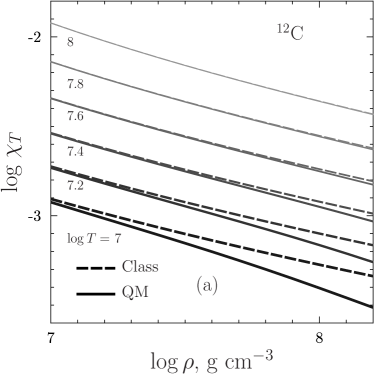
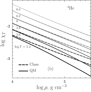
Figure 3: Logarithm of compressibility $\chi_{T}$ of isothermal WD matter composed of ¹²C (a) or ⁴He (b) as a function of $\log\rho$ for several values of temperature. Solid (dashed) curves include (exclude) quantum effects in the Coulomb liquid of ions.

The compressibilities $\chi_{\rho}$ and $\chi_{T}$ are interesting not only for WD seismology. In particular they determine the adiabatic gradient $\nabla_{\rm ad}$ which regulates convective stability of stellar matter. Evidently, in degenerate WD cores $\chi_{\rho}$ is mainly determined by the bulk pressure of degenerate electrons; it is affected by the state of ions but only weakly. On the contrary, $\chi_{T}$ is mainly determined by ions. It is plotted in Fig. 3 as a function of mass density for carbon (a) and helium (b) matter at several temperatures above melting. Note that the scale of the vertical axis is logarithmic. Solid lines are calculated using full equation (14) while dashed lines are respective classic values. Quantum effects are seen to decrease $\chi_{T}$. As in the case of the heat capacity, the strongest decrease occurs in deeper WD layers and at lower temperatures.

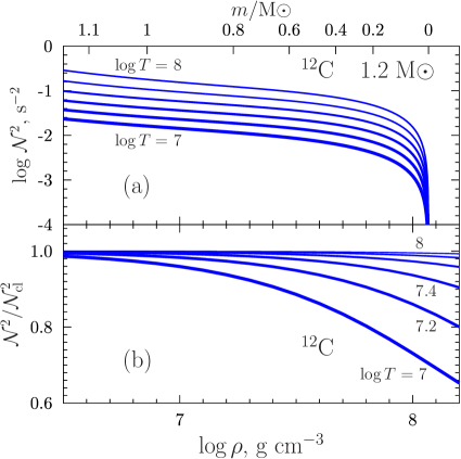
Figure 4: (a) Logarithm of the squared Brunt-Väisälä frequency in the carbon core of an isothermal 1.2 M$\odot$ WD as a function of mass density for six values of the core temperature, from $T=10^{7}$ to $10^{8}$ K. The upper horizontal scale displays accumulated stellar mass $m$. (b) The ratio of squared Brunt-Väisälä frequencies calculated including and neglecting quantum effects of ions versus $\rho$ at the same temperatures.

Fig. 4(a) shows the density dependence of squared Brunt-Väisälä frequency in the central part of an isothermal carbon core of a 1.2 M$\odot$ WD as a function of density $\rho$ at six selected temperatures, with $\log T$ [K]=7, 7.2, …8. The upper horizontal axis displays values of stellar mass $m$ (in units of M$\odot$) accumulated in spheres restricted by respective $\rho$. To demonstrate the importance of quantum effects of ions, Fig. 4(b) shows the ratio of the squared Brunt-Väisälä frequency with quantum effects to that without quantum effects as a function of mass density at the same $T$. Since gravity cancels out, this becomes a universal function of density, temperature, and composition and does not depend on a particular WD model. Ion quantum effects lower ${\cal N}$ and actual $g$-mode frequencies.

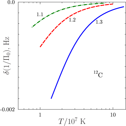
Figure 5: Variation of $\Pi_{0}^{-1}$ that determines frequency difference between two $g$-modes with large successive numbers of radial nodes ($k$, $k+1\gg 1$) under the effect of quantum effects of ions as a function of core temperature for carbon WDs with $M=$1.1, 1.2 and 1.3 M$\odot$. At low $T$ the curves are broken at onset of crystallization in the WD center.

In order to gauge the effect of these differences on the pulsational properties of WDs we consider the asymptotic period spacing (e.g., De Gerónimo et al., 2019) between pulsation modes with fixed multipolarity $\ell$ and azimuthal number $m$ but succesive numbers $k$ and $k+1$ of radial nodes in the limit of large $k$,

$$\Delta\Pi_{l}^{\rm a} = \Pi_{0}/\sqrt{\ell(\ell+1)}~{},$$ (27)

$$\Pi_{0} = 2{\rm\pi}^{2}\left[\int_{0}^{R}{\rm d}r\,\frac{\cal N}{r}\right]^{-1}~{}.$$ (28)

According to Fig. 4(b), the difference between ${\cal N}$ and ${\cal N}_{\rm cl}$ vanishes while still at fairly high densities. This allows us to calculate the quantity

$$\delta\left(\frac{1}{\Pi_{0}}\right)=\frac{1}{2\pi^{2}}\int_{0}^{R}{\rm d}r\,\frac{({\cal N}-{\cal N}_{\rm cl})}{r},$$ (29)

which is insensitive to thermodynamics in the WD envelope and outer core. This quantity determines the magnitude of eigenmode frequency change originating from the quantum phenomena in the ion liquid near the WD center. In Fig. 5, $\delta(\Pi_{0}^{-1})$ is plotted as a function of core temperature (in units of $10^{7}$ K, above melting) for carbon WDs of masses 1.1, 1.2, and 1.3 M$\odot$. According to numerical data of De Gerónimo et al. (2019), the range of realistic values of $\Delta\Pi_{1}^{\rm a}$ can be roughly estimated as $\sim 5$–50 s. Per equation (27) with $\ell=1$, this translates into $\Pi_{0}^{-1}\sim 14$–140 mHz which should be compared with the expected variation displayed in Fig. 5. Given the remarkable accuracy of seismological measurements, an experimental verification of spectral variations due to quantum effects predicted in Fig. 5 seems feasible.

3.3 Radii of low-mass WDs with He cores

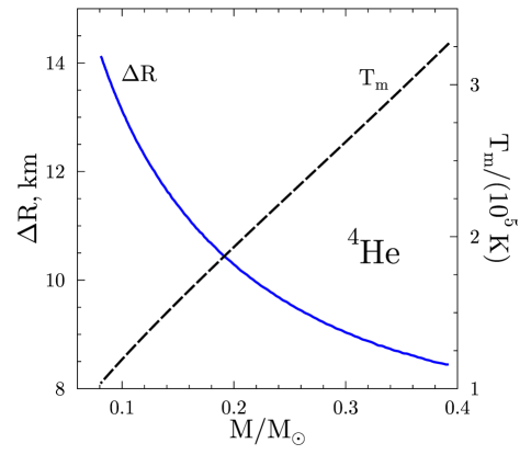
Figure 6: Radius increase $\Delta R$ (solid line) due to quantum ion effects for WDs with ⁴He cores versus WD mass. In each case the temperature of the isothermal core corresponds to the crystallization in the WD center $T=T_{\rm m}$. This temperature is plotted by the dashed line along the right vertical axis.

Here we comment on the importance of ion quantum effects for hydrostatic models of low-mass WDs. To this aim, we have calculated a sequence of WD models of different masses $M$ with isothermal helium cores, from 0.1 M$\odot$ to 0.4 M$\odot$. In doing so we have taken into account the ion pressure at a finite core temperature $T$. This temperature has been set equal to the crystallyzation temperature in the WD center (the lowest temperature at which the entire core remains liquid). This temperature increases with the growth of $M$ and is shown by a dashed curve in Fig. 6 referring to the right vertical axis. For each $M$, we have calculated WD models twice: including quantum term in the ion pressure (9) and assuming purely classic ions.

Fig. 6 presents the difference of WD radii $\Delta R$, calculated with and without ion quantum effects versus mass $M$. The ion pressure is much smaller than the electron one and the quantum contribution to the ion pressure is, in turn, smaller than the absolute magnitude of the ion electrostatic contribution. Nevertheless, the difference due to quantum effects is seen to be $\sim 10$ km. Somewhat counterintuitively, it increases with decreasing mass, i.e. $\Delta R$ is larger for more classic extremely low-mass helium stars! The decrease is associated with two effects, a decrease of $|P_{i}|/P_{e}$ when $\rho$ increases in heavier stars and a general increase of $R$ with decrease of $M$.

The effect is small but may be important for AM Canum Venaticorum variables (AM CVn) which constitute a class of binaries with extremely short orbital periods (down to a few minutes); e.g., see Deloye et al. (2007); Solheim (2010); Ramsay et al. (2018). Their evolution is governed by mass transfer from a donor star to an accreting WD as well as by orbital momentum loss due to gravitational wave emission. We are interested in the scenario where the donor is a low-mass ($M\lesssim 0.4$ M$\odot$) He dwarf. It can be very cold ($T_{\rm s}$ as low as $\sim 1000$ K, see Deloye et al. 2007). In the process of accretion, it loses mass and moves to the left in Fig. 6 so that the predicted $\Delta R$ due to quantum effects increases. Thus accurate incorporation of these effects may be crucial to correctly model the final outcome of the evolution, in particular, when or whether there will be a direct impact and merger.

4 Conclusion

In Section 2, we present a simple analytical formula, equation (4), which accurately approximates calculations of the energy of a quantum OCP of ions in a uniform electron background. The calcuations were performed in Paper I from first principles in the regime of a strongly-coupled liquid ($1\leq\Gamma\leq 175$) neglecting the effects of quantum statistics of ions. At $\Gamma<1$, equation (4) reduces to the familiar expression for a classic liquid (Potekhin & Chabrier, 2000) combined with the first Wigner-Kirkwood correction. In this way equation (4) stays valid at small $\Gamma$.

Equation (4) allows one to construct accurate analytic thermodynamics of ionic OCP at $\Gamma\leq 175$, obtain an analytic expression for the Helmholtz free energy, equation (12), and calculate temperature and density derivatives which are required for finding various thermodynamic quatities for astrophysical applications.

In Section 3, we apply the results for constructing major thermodynamic quantities in an OCP of ions immersed in a degenerate gas of electrons (including Sommerfeld temperature corrections for electron thermodynamic quantities). This is a good model to describe dense matter in degenerate cores of WDs with account of quantum effects in ion motion. We apply this formalism to investigate the ionic quantum effects on the total heat capacity of WDs, compressibilities $\chi_{T}$ and $\chi_{\rho}$, Brunt-Väisälä frequency of WDs, and radii of low-mass WDs with helium cores. Our main conclusion is that quantum effects of ions become really important in central regions of WD cores at low enough temperatures (within a factor of a few of the crystallization temperature). In general, the strongest effects occur in WDs with massive helium or carbon cores. In particular, quantum effects can noticeably decrease the heat capacity and accelerate cooling of massive WDs with carbon cores prior to crystallization. The only exception to this general trend is an increase of the quantum correction to the radius of a helium WD, $\Delta R$, with decrease of its mass (Fig. 6).

The theory we present is valid for quantum OCP of ions neglecting ion exchange effects which are not relevant for applications. Further work is required to elaborate this theory by studying quantum anharmonic corrections to the harmonic-lattice model of a crystallized phase and by developing detailed theory of quantum ion mixtures.

References

- Baiko (2019) Baiko D. A., 2019, MNRAS, 488, 5042
- Baiko et al. (2001) Baiko D. A., Potekhin A. Y., Yakovlev D. G., 2001, Phys. Rev. E, 64, 057402
- Bergeron et al. (2019) Bergeron P., Dufour P., Fontaine G., Coutu S., Blouin S., Genest-Beaulieu C., Bédard A., Rolland B., 2019, ApJ, 876, 67
- Bischoff-Kim et al. (2019) Bischoff-Kim A., et al., 2019, ApJ, 871, 13
- Blouin et al. (2019) Blouin S., Dufour P., Thibeault C., Allard N. F., 2019, ApJ, 878, 63
- Brassard et al. (1991) Brassard P., Fontaine G., Wesemael F., Kawaler S. D., Tassoul M., 1991, ApJ, 367, 601
- Córsico et al. (2019) Córsico A. H., Althaus L. G., Miller Bertolami M. M., Kepler S. O., 2019, arXiv e-prints, p. arXiv:1907.00115
- De Gerónimo et al. (2019) De Gerónimo F. C., Córsico A. H., Althaus L. G., Wachlin F. C., Camisassa M. E., 2019, A&A, 621, A100
- Deloye et al. (2007) Deloye C. J., Taam R. E., Winisdoerffer C., Chabrier G., 2007, MNRAS, 381, 525
- Dewitt & Slattery (1999) Dewitt H., Slattery W., 1999, Contributions to Plasma Physics, 39, 97
- Fernandes et al. (2019) Fernandes C. S., Van Grootel V., Salmon S. J. A. J., Aringer B., Burgasser A. J., Scuflaire R., Brassard P., Fontaine G., 2019, ApJ, 879, 94
- Genest-Beaulieu & Bergeron (2019) Genest-Beaulieu C., Bergeron P., 2019, ApJ, 871, 169
- Haensel et al. (2007) Haensel P., Potekhin A. Y., Yakovlev D. G., 2007, Neutron Stars. 1. Equation of State and Structure. Springer, New York
- Jones & Ceperley (1996) Jones M. D., Ceperley D. M., 1996, Phys. Rev. Lett., 76, 4572
- Kepler et al. (2019) Kepler S. O., et al., 2019, MNRAS, 486, 2169
- Lamb & van Horn (1975) Lamb D. Q., van Horn H. M., 1975, ApJ, 200, 306
- Landau & Lifshitz (1980) Landau L. D., Lifshitz E. M., 1980, Statistical Physics. Part I. Course of theoretical physics, Oxford: Pergamon Press
- Pelisoli & Vos (2019) Pelisoli I., Vos J., 2019, MNRAS, 488, 2892
- Potekhin & Chabrier (2000) Potekhin A. Y., Chabrier G., 2000, Phys. Rev. E, 62, 8554
- Ramsay et al. (2018) Ramsay G., et al., 2018, A&A, 620, A141
- Shapiro & Teukolsky (1983) Shapiro S. L., Teukolsky S. A., 1983, Black holes, white dwarfs, and neutron stars: The physics of compact objects. Wiley-Interscience, New York
- Solheim (2010) Solheim J. E., 2010, PASP, 122, 1133
- Swarzschild (1958) Swarzschild M., 1958, Structure and Evolution of the Stars. Cambridge Univ. Press, Cambridge
- Tremblay et al. (2019) Tremblay P.-E., et al., 2019, Nature, 565, 202
- Winget & Kepler (2008) Winget D. E., Kepler S. O., 2008, ARA&A, 46, 157