Unified description of turbulent entrainment

Abstract

We present a mathematical description of turbulent entrainment that is applicable to free shear problems that evolve in space, time or both. Defining the global entrainment velocity $\makebox[0.0pt]{$\phantom{V}\overline{\phantom{V}}$}V_{g}$ to be the fluid motion across an isosurface of an averaged scalar, we find that for a slender flow, $\makebox[0.0pt]{$\phantom{V}\overline{\phantom{V}}$}V_{g}=\overline{u}_{\zeta}-\overline{D}h_{t}/\overline{D}t$, where $\overline{D}/\overline{D}t$ is the material derivative of the average flowfield and $\overline{u}_{\zeta}$ is the average velocity perpendicular to the flow direction across the interface located at $\zeta=h_{t}$. The description is shown to reproduce well-known results for the axisymmetric jet, the planar wake and the temporal jet, and provides a clear link between the local (small-scale) and global (integral) descriptions of turbulent entrainment. Application to unsteady jets/plumes demonstrates that, under unsteady conditions, the entrainment coefficient $\alpha$ no longer only captures entrainment of ambient fluid, but also time-dependency effects due to the loss of self-similarity.

1 Introduction

Despite over half a century of research and several review articles (e.g. Turner, 1986; Fernando, 1991; Woods, 2010; de Rooy, 2013; Da Silva et al., 2014; Mellado, 2017), our understanding of turbulent entrainment (the transport of fluid from regions of relatively low to relatively high levels of turbulence) remains fragmented. One important reason is that turbulent entrainment is notoriously difficult to determine. Entrainment is a process that typically occurs over much larger timescales than turbulent timescales, and its effects are therefore easily obfuscated by turbulent fluctuations and transient effects. Furthermore, the quantification of turbulent entrainment requires the determination of a turbulent and non-turbulent (or less turbulent) region which is, by definition, arbitrary and thus subject to uncertainty.

However, there are other reasons that the understanding of turbulent entrainment remains challenging. One challenge is the sheer number of flows in which turbulent entrainment plays a role. Developing boundary layers can be classified based on the number of independent variables on which their solution depends, with a further distinction between statistically steady and unsteady problems, as shown in table 1. Consider a turbulent velocity field $\boldsymbol{u}(x,y,z,t)$, which will generally not have any symmetries. By ensemble averaging this velocity field, denoted by $\overline{\cdot}$, an average velocity field $\overline{\boldsymbol{u}}$ is obtained which satisfies the symmetries present in the problem formulation (such as axisymmetric or streamwise homogeneity). In table 1, $x$ is the (slowly developing) streamwise direction, and $z$ or $r$ is the normal direction, where $z$ would be used for planar problems and $r$ for axisymmetric problems. Finally, the class of steady problems with two independent variables comprises e.g. planar and axisymmetric jets (Hussein et al., 1994; Da Silva & Métais, 2002; Westerweel et al., 2005; Watanabe et al., 2014), plumes (List, 1982), wakes (Cantwell & Coles, 1983; Obligado et al., 2016), fountains (Hunt & Burridge, 2015), boundary layers (Head, 1958; Sillero et al., 2013), mixing layers (Rajaratnam, 1976) and inclined gravity currents (Wells et al., 2010; Odier et al., 2014; Krug et al., 2015).

In the class of unsteady problems with two independent variables are problems that develop slowly in time in one spatial dimension $z$ or $r$. These are problems such as penetrative convection (Mellado, 2012; Holzner & van Reeuwijk, 2017), convective and stable boundary layers (as relevant to the atmospheric boundary layer and the oceanic mixed layer; Kato & Phillips, 1969; Deardorff et al., 1980; Sullivan et al., 1998; Jonker et al., 2013; Garcia & Mellado, 2014), stratocumulus clouds (Mellado, 2017), but also include temporal jets (Da Silva & Pereira, 2008; van Reeuwijk & Holzner, 2014), plumes (Krug et al., 2017), gravity currents (van Reeuwijk et al., 2018, 2019), wakes (Redford et al., 2012; Watanabe et al., 2016), mixing layers (Watanabe et al., 2018a) and compressible reacting mixing layers (Jahanbakhshi & Madnia, 2018). These temporal flows are not generally encountered in nature but share many of the features of their 2D steady cousins. However, with two homogeneous spatial directions, they are ideal for exploration with direct numerical simulation.

Steady problems with three independent variables possess two normal directions in which the flow develops ‘fast’ but in an anisotropic manner. Examples are jets and plumes discharged vertically in a crosswind (Mahesh, 2013; De Wit et al., 2014; Woods, 2010; Devenish et al., 2010), stratified wakes (Xu et al., 1995) and horizontally discharged point releases in stratified layers. The class of unsteady problems with three independent variables comprises all the flows mentioned in the category of 2D steady developing boundary layers, provided that one of their boundary conditions or the environment changes in time. Examples include unsteady jets and plumes (Scase et al., 2006; Craske & van Reeuwijk, 2015, 2016; Woodhouse et al., 2016) and starting plumes (Turner, 1962). The class of unsteady problems with four independent variables comprises unsteady versions in the category of 3D steady free shear flows. These comprise unsteady gravity currents from a point source, and unsteady jets/plumes in a cross-flow.

Table 1: Classification of free shear flows based on the number of independent variables.

Dims	Steady	Unsteady
1	$\overline{\boldsymbol{u}}(z)$ (not encountered in free shear flows)	$\overline{\boldsymbol{u}}(t)$ (not encountered in free shear flows)
2	$\overline{\boldsymbol{u}}(x,z)$, $\overline{\boldsymbol{u}}(x,r)$ jets, wakes, mixing layers, plumes, inclined gravity currents, $\ldots$	$\overline{\boldsymbol{u}}(z,t)$, $\overline{\boldsymbol{u}}(r,t)$ Temporal jets, wakes, mixing layers, plumes, inclined gravity currents, penetrative convection, convective boundary layer, $\ldots$
3	$\overline{\boldsymbol{u}}(x,y,z)$ gravity currents from a point source, stratified wakes, jets and plumes in crossflow, $\ldots$	$\overline{\boldsymbol{u}}(x,z,t)$, $\overline{\boldsymbol{u}}(x,r,t)$ Unsteady versions of those in the category of 2D steady flows, e.g. unsteady jets, plumes, $\ldots$
4		$\overline{\boldsymbol{u}}(x,y,z,t)$ Unsteady versions of those in the category of 3D steady flows, e.g. gravity currents from a point source with variable discharge, $\ldots$

Turbulent entrainment is generally studied either from a local or a global perpective. The global approach involves inferring the entrainment velocity from the Reynolds-averaged equations (e.g. Turner, 1986; Townsend, 1976) and considers entrainment from an integral perpective. The local approach, as pioneered by Corrsin & Kistler (1955), considers the microscale perspective. The local approach starts from choosing a scalar quantity $\chi$ to provide an implicit definition of the instantaneous turbulent-nonturbulent interface (TNTI), where a threshold value $\chi_{0}$ is used to distinguish the turbulent zone ($\chi\geq\chi_{0}$) from the nonturbulent zone ($\chi<\chi_{0}$). The most commonly used scalar quantity is enstrophy (e.g. Bisset et al., 2002; Holzner & Luethi, 2011; Da Silva et al., 2014; van Reeuwijk & Holzner, 2014), which is consistent with Corrsin & Kistler (1955), but passive scalars (e.g. Sreenivasan et al., 1989; Westerweel et al., 2005; Burridge et al., 2017) or the turbulence kinetic energy (Philip et al., 2014; Chauhan et al., 2014) are also used to define the TNTI. Note however that care needs to be taken when using turbulence kinetic energy to delineate the TNTI, as pressure can induce irrotational velocity fluctuations in the ambient (Watanabe et al., 2018b).

The choice of the threshold value $\chi_{0}$ is always slightly arbitrary, as the flow transitions smoothly from turbulent to non-turbulent. In addition any measurement and simulation data are subject to uncertainty, and background levels of $\chi$ may be nonzero (e.g. enstrophy levels in a turbulent ambient). One therefore typically chooses a small and finite nonzero threshold $\chi_{0}$ to define the TNTI. Since the interface between turbulent and non-turbulent fluid is generally very sharp, there is a range of thresholds $\chi_{0}$ that can be chosen for which the entrainment statistics are insensitive to the choice of $\chi_{0}$ (Da Silva et al., 2014).

The velocity $\boldsymbol{v}$ associated with any trajectory on an isosurface of $\chi$ satisfies

$$\frac{\textnormal{d}\chi}{\textnormal{d}t}=\frac{\partial\chi}{\partial t}+\boldsymbol{v}\cdot\boldsymbol{\nabla}\chi=0.$$ (1)

By introducing a relative velocity $\boldsymbol{V}=\boldsymbol{v}-\boldsymbol{u}$, which is the difference between the isosurface velocity $\boldsymbol{v}$ and the fluid velocity $\boldsymbol{u}$, (1) can be rewritten as (Dopazo et al., 2007; Holzner & Luethi, 2011)

$$V_{n}=-\frac{1}{|\boldsymbol{\nabla}\chi|}\frac{D\chi}{Dt},$$ (2)

where $D/Dt=\partial/\partial t+\boldsymbol{u}\cdot\boldsymbol{\nabla}$ is the material derivative, $V_{n}=\boldsymbol{V}\cdot\boldsymbol{N}$ is the normal component of the relative velocity and $\boldsymbol{N}=\boldsymbol{\nabla}\chi/|\boldsymbol{\nabla}\chi|$ is the (3D) normal vector pointing into the turbulent region (Figure 1(a)). Note that the other two components of $\boldsymbol{V}$ tangential to the isosurface are not specified by this definition. For an entraining flow, $V_{n}<0$, which is a consequence of defining a normal $\boldsymbol{N}$ that points into $\Omega$. The inward pointing normal also has consequences for the Gauss divergence theorem. By substituting the governing equation for $\chi$ (usually enstrophy) into (2) and averaging, local aspects of turbulent entrainment can be explored (e.g. Holzner & Luethi, 2011; Da Silva et al., 2014; van Reeuwijk & Holzner, 2014; Krug et al., 2015; Jahanbakhshi & Madnia, 2018).

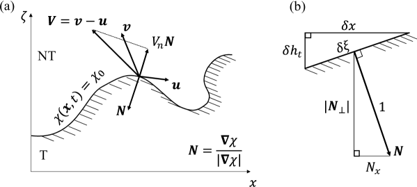
Figure 1: Interface properties of the turbulent-nonturbulent interface (TNTI) separating turbulent (T) from non-turbulent (NT) fluid. (a) Definition sketch. (b) Geometric properties.

The global entrainment velocity $\makebox[0.0pt]{$\phantom{V}\overline{\phantom{V}}$}V_{g}$ is not as uniquely defined as the local entrainment velocity (2) (Turner, 1986; Hunt et al., 1983). For spatially developing flows, the entrainment velocity is usually associated with a flow into the turbulent region. For temporal problems however, it is defined via $\textnormal{d}h/\textnormal{d}t$, the growth of the layer in time, where $h$ is some characteristic layer thickness. However, for spatially developing flows in which the environment is non-quiescent or is stratified, there is another mode of entrainment which is associated with the entrainment across the boundary. These different forms of entrainment were discussed in Hunt et al. (1983); Turner (1986) and cause confusion between disciplines, as they describe related processes that are not necessarily equivalent. In this paper we derive an unambiguous definition of the global entrainment velocity that can be used for spatial, temporal and spatio-temporal (unsteady) entrainment problems.

The aim of this paper is to derive an integral description of free shear flows capable of representing both the local and global viewpoints of turbulent entrainment. An equivalent definition to (2) is presented for the global entrainment velocity. The framework provides a unified description of entrainment in temporal problems (2D unsteady; Da Silva & Pereira, 2008; van Reeuwijk & Holzner, 2014; Krug et al., 2017), in which the TNTI moves but there is no net flow into the turbulent layer ($V_{n}$ produced by $\boldsymbol{v}$), spatial problems (2D steady; Rajaratnam, 1976; Turner, 1986; Philip et al., 2014), in which the TNTI is statistically steady but there is a net flow into the turbulent layer ($V_{n}$ produced by $\boldsymbol{u}$), and unsteady free shear layers (3D unsteady; Craske & van Reeuwijk, 2016).

This paper is organised as follows. §2 introduces the integral operator identities and the averaged plane-integrated Navier-Stokes equations which describe the integral spatio-temporal dynamics of free shear flows. In §3, an average isosurface of $\overline{\chi}$ is applied to the equations which results in an expression for the global entrainment velocity $\makebox[0.0pt]{$\phantom{V}\overline{\phantom{V}}$}V_{g}$ in terms of an explicit function $h_{t}$ describing the TNTI. The implications of this new definition of $\makebox[0.0pt]{$\phantom{V}\overline{\phantom{V}}$}V_{g}$ are discussed in §4. Four canonical free shear flows (an axisymmetric jet, a planar wake, a temporal jet and an unsteady jet/plume) are studied in §5 to show that the current definition of $\makebox[0.0pt]{$\phantom{V}\overline{\phantom{V}}$}V_{g}$ is fully consistent with previous results. Application of the new description to unsteady jets and plumes reveals the relation between the entrainment coefficient $\alpha$ and actual entrainment across the interface. Concluding remarks are made in §6.

2 Local averaged integral equations

In this section we present integral volume (i.e. continuity) and momentum conservation equations. The focus of this work is on turbulent free shear flows which develop slowly (in a statistical sense) in time $t$, in the spatial direction $x$, or both. The incompressible Navier-Stokes equations are given by

$$\boldsymbol{\nabla}\cdot\boldsymbol{u} =0,$$ (3)

$$\frac{D\boldsymbol{u}}{Dt} =-\frac{1}{\rho_{0}}\boldsymbol{\nabla}p+\boldsymbol{\nabla}\cdot\boldsymbol{\tau}+\boldsymbol{f},$$ (4)

where $\boldsymbol{\tau}$ denotes the viscous stress tensor and $\boldsymbol{f}$ is a body force. These equations will be integrated over the turbulent region in the $y-z$ plane which is denoted $\Omega$. The following identities for the integrals of the gradient, divergence and material derivative operators can be derived:

$$\int_{\Omega}\boldsymbol{\nabla}\phi\textnormal{d}A =\frac{\partial}{\partial x}\int_{\Omega}\phi\textnormal{d}A\boldsymbol{e}_{x}-\oint_{\partial\Omega}\phi\frac{\boldsymbol{N}}{|\boldsymbol{N}_{\perp}|}\textnormal{d}\ell,$$ (5)

$$\int_{\Omega}\boldsymbol{\nabla}\cdot\boldsymbol{F}\textnormal{d}A =\frac{\partial}{\partial x}\int_{\Omega}F_{x}\textnormal{d}A-\oint_{\partial\Omega}\boldsymbol{F}\cdot\frac{\boldsymbol{N}}{|\boldsymbol{N}_{\perp}|}\textnormal{d}\ell,$$ (6)

$$\int_{\Omega}\frac{D\phi}{Dt}\textnormal{d}A =\frac{\partial}{\partial t}\int_{\Omega}\phi~{}\textnormal{d}A+\frac{\partial}{\partial x}\int_{\Omega}u_{x}\phi~{}\textnormal{d}A-\int_{\Omega}\phi\boldsymbol{\nabla}\cdot\boldsymbol{u}\textnormal{d}A+\oint_{\partial\Omega}\frac{V_{n}}{|\boldsymbol{N}_{\perp}|}\phi~{}\textnormal{d}\ell,$$ (7)

where $\phi$ is an arbitrary scalar or vector component field and $\boldsymbol{F}$ is an arbitrary vector field. Vectors with a perp ($\perp$) subscript denote the components perpendicular to the $x$-direction, i.e. $\boldsymbol{F}=[F_{x},\boldsymbol{F}_{\perp}]^{T}$, and $\boldsymbol{\nabla}_{\perp}=[\partial/\partial y,\partial/\partial z]^{T}$. The unit vector $\boldsymbol{N}=\boldsymbol{\nabla}\chi/|\boldsymbol{\nabla}\chi|$ is normal to the 3D surface $\chi=\chi_{0}$ which demarcates between turbulent and non-turbulent regions. The normal vector can be written as $\boldsymbol{N}=[N_{x},\boldsymbol{N}_{\perp}]^{T}$, so that $|\boldsymbol{N}_{\perp}|$ is the magnitude of the 3D normal in the $y-z$ plane [see figure 1(b)]. Finally, $\boldsymbol{e}_{x}$ is the unit vector in the $x$-direction and $u_{x}$ is the component of the fluid velocity field $\boldsymbol{u}$ in that same direction. An easily accessible yet rigorous proof of these three identities is given in Appendix A. A more general derivation using differential geometry, which highlights the role of Stokes’ theorem and the Leibniz integral rule, is given in Appendix B.

Since the flow is turbulent, the integration domain $\Omega(y,z;x)$ can consist of several disconnected blobs of turbulent fluid, i.e. $\Omega=\Omega_{1}\cup\Omega_{2}\cup\ldots$. This implies that the domain boundary $\partial\Omega$ contains multiple closed trajectories $\partial\Omega_{1},\partial\Omega_{2},\ldots$ which are summed up with the line integral, That is, $\oint_{\partial\Omega}\cdot\textnormal{d}\ell=\oint_{\partial\Omega_{1}}\cdot\textnormal{d}\ell+\oint_{\partial\Omega_{2}}\cdot\textnormal{d}\ell+\ldots$ if the domain contains multiple disconnected blobs.

Noting that $\boldsymbol{\nabla}\cdot\boldsymbol{u}=D\phi/Dt=0$ for $\phi=1$ and using (7) implies that the instantaneous integral continuity equation is given by

$$\frac{\partial}{\partial t}\int_{\Omega}~{}\textnormal{d}A+\frac{\partial}{\partial x}\int_{\Omega}u_{x}~{}\textnormal{d}A=-\oint_{\partial\Omega}\frac{V_{n}}{|\boldsymbol{N}_{\perp}|}~{}\textnormal{d}\ell.$$ (8)

Note that if the relative isosurface velocity $\boldsymbol{V}$ is everywhere tangential to the interface then $V_{n}=0$, in which case (8) describes a streamtube. Entrainment allows exchange across the isosurface $\chi=\chi_{0}$. For an entraining flow, $V_{n}<0$ (due to the inward pointing normal).

The line integral represents the net entrainment into the turbulent region. The factor $|\boldsymbol{N}_{\perp}|$ accounts for the projection of the 3D quantity $V_{n}$ onto the $y-z$ plane. This is better seen by using $V_{n}=\boldsymbol{V}\cdot\boldsymbol{N}$ to write the entrainment term as

$$\oint_{\partial\Omega}\frac{V_{n}}{|\boldsymbol{N}_{\perp}|}~{}\textnormal{d}\ell=\oint_{\partial\Omega}\boldsymbol{V}_{\perp}\cdot\boldsymbol{n}~{}\textnormal{d}\ell+\oint_{\partial\Omega}V_{x}\frac{N_{x}}{|\boldsymbol{N}_{\perp}|}~{}\textnormal{d}\ell,$$ (9)

where $\boldsymbol{n}=\boldsymbol{\nabla}_{\perp}\chi/|\boldsymbol{\nabla}_{\perp}\chi|$ is the normal in the $y-z$ plane, and note that this quantity is related to the 3D normal via $\boldsymbol{n}=\boldsymbol{N}_{\perp}/|\boldsymbol{N}_{\perp}|$. The first term on the right-hand side of (9) is simply the entrainment flux arising from the in-plane relative velocity components $\boldsymbol{V}_{\perp}$. As described in appendices A and B, the second term on the right-hand side of (9) arises from the commutation of integration and differiation with respect to $x$ that is required to formulate (8). It represents the net transport of the streamwise relative velocity component $V_{x}$ into the turbulent region across the interface whose local slope is $N_{x}/|\boldsymbol{N}_{\perp}|$ (see Figure 1). We note that $|\boldsymbol{N}_{\perp}|$ can be zero locally when $\boldsymbol{N}$ is aligned with the $x$-direction , which would render the integrand infinite. This is an inescapable consequence of determining entrainment as a function of $x$. Any subsequent integration over $x$ will remain finite however, since $V_{n}/|\boldsymbol{N}_{\perp}|\textnormal{d}\ell\textnormal{d}x=V_{n}\textnormal{d}S$ where $\textnormal{d}S$ is the local surface area of the surface in 3D.

Integration over the region $\Omega$ of (4) and use of identities (5)-(7) results in

$$\begin{split}\frac{\partial}{\partial t}\int_{\Omega}\boldsymbol{u}~{}\textnormal{d}A&+\frac{\partial}{\partial x}\int_{\Omega}\left(u_{x}\boldsymbol{u}+\frac{p}{\rho_{0}}\boldsymbol{e}_{x}\right)~{}\textnormal{d}A=\\ &-\oint_{\partial\Omega}\frac{1}{|\boldsymbol{N}_{\perp}|}\left(V_{n}\boldsymbol{u}-\frac{p}{\rho_{0}}\boldsymbol{N}\right)~{}\textnormal{d}\ell+\int_{\Omega}\boldsymbol{f}\textnormal{d}A.\end{split}$$ (10)

Here, the shear-stress contributions have been neglected as is conventional for high Reynolds free shear flows. Equations (8) and (10) are instantaneous.

Performing ensemble averaging, denoted by the overbar $\overline{\cdot}$, on the instantaneous integrated continuity equation (8) and the streamwise $x-$component of the integrated momentum equation (10) yields

$$\frac{\partial}{\partial t}{\overline{\int_{\Omega}~{}\textnormal{d}A}}+\frac{\partial}{\partial x}\overline{\int_{\Omega}u_{x}~{}\textnormal{d}A}=-\overline{\oint_{\partial\Omega}\frac{V_{n}}{|\boldsymbol{N}_{\perp}|}~{}\textnormal{d}\ell},$$ (11)

$$\begin{split}\frac{\partial}{\partial t}\overline{\int_{\Omega}u_{x}~{}\textnormal{d}A}&+\frac{\partial}{\partial x}\overline{\int_{\Omega}\left(u_{x}^{2}+\frac{p}{\rho_{0}}\right)~{}\textnormal{d}A}=\\ &-\overline{\oint_{\partial\Omega}\frac{1}{|\boldsymbol{N}_{\perp}|}\left(V_{n}u_{x}-\frac{p}{\rho_{0}}N_{x}\right)~{}\textnormal{d}\ell}+\overline{\int_{\Omega}f_{x}\textnormal{d}A}.\end{split}$$ (12)

In the integral continuity equation (11), $\overline{\int_{\Omega}\textnormal{d}A}$ represents the average instantaneous cross-sectional area of the turbulent region at location $x$. It is not possible to commute the integral with the ensemble averaging because the integration regions $\Omega$ and $\partial\Omega$ vary in time and per ensemble instance.

3 Global averaged integral equations

Equations (11), (12) ultimately link the integral behaviour of the free shear flow to the small-scale dynamics at the TNTI when $\chi$ is an instantaneous quantity. The global, integral dynamics can be obtained by using an average quantity $\overline{\chi}$, with associated threshold $\overline{\chi}_{0}$, to identify the interface (Figure 2). By considering an average quantity, the TNTI will not be contorted but will be smooth and satisfy the symmetries corresponding to homogeneity in the problem under consideration.

3.1 Non-slender flows

We define the global entrainment velocity $\makebox[0.0pt]{$\phantom{V}\overline{\phantom{V}}$}V_{g}$ to be the net transport across an averaged scalar $\overline{\chi}$. This implies that the 3D normal is defined as $\boldsymbol{N}_{g}=\boldsymbol{\nabla}\overline{\chi}/|\boldsymbol{\nabla}\overline{\chi}|$, and therefore that

$$V_{g}=({\boldsymbol{v}}-{\boldsymbol{u}})\cdot\boldsymbol{N}_{g}=\frac{{\boldsymbol{v}}\cdot\boldsymbol{\nabla}\overline{\chi}-{\boldsymbol{u}}\cdot\boldsymbol{\nabla}\overline{\chi}}{|\boldsymbol{\nabla}\overline{\chi}|}=-\frac{1}{|\boldsymbol{\nabla}\overline{\chi}|}\frac{D\overline{\chi}}{Dt},$$ (13)

where use was made of (1) for $\chi=\overline{\chi}$. The equation above is the instantaneous global entrainment velocity across an isosurface based on a Reynolds-averaged quantity. The mean entrainment velocity can be determined by applying Reynolds-averaging to (13), with result

$$\makebox[0.0pt]{$\phantom{V}\overline{\phantom{V}}$}V_{g}=\overline{\boldsymbol{V}\cdot\boldsymbol{N}_{g}}=\overline{\boldsymbol{V}}\cdot\boldsymbol{N}_{g}=-\frac{1}{|\boldsymbol{\nabla}\overline{\chi}|}\frac{\overline{D}\overline{\chi}}{\overline{D}t},$$ (14)

where $\overline{D}/\overline{D}t=\partial/\partial t+\overline{\boldsymbol{u}}\cdot\boldsymbol{\nabla}$.

An advantage of considering averaged quantities is that it is possible to represent the isosurface $\overline{\chi}=\overline{\chi}_{0}$ (which implicitly defines the TNTI) explicitly in terms of a single-valued function $h_{t}$ in a coordinate system appropriately representing the symmetries of the free-shear problem under consideration. Restricting attention to planar or axisymmetric problems, a scalar level-set function $L(x,\zeta,t)=h_{t}(x,t)-\zeta$ can be constructed such that $L=0$ represents the average interface position where $\zeta$ is the direction normal to the $x$-direction. Setting $\overline{\chi}=L$ implies that (13) can equivalently be expressed as

$$\makebox[0.0pt]{$\phantom{V}\overline{\phantom{V}}$}V_{g}=-\frac{1}{|\boldsymbol{\nabla}L|}\left(\frac{\overline{D}h_{t}}{\overline{D}t}-\frac{\overline{D}\zeta}{\overline{D}t}\right)=\frac{1}{|\boldsymbol{\nabla}L|}\left(\overline{u}_{\zeta}-\frac{\overline{D}h_{t}}{\overline{D}t}\right),$$ (15)

where $|\boldsymbol{\nabla}L|=\sqrt{1+(\partial h_{t}/\partial x)^{2}}$.

Because the interface is based on the average quantity $\overline{\chi}$, the averaging and integral operators do commute, which implies that (11), (12) simplify to

$$\frac{\partial}{\partial t}{\int_{\overline{\Omega}}\textnormal{d}A}+\frac{\partial}{\partial x}\int_{\overline{\Omega}}\overline{u}_{x}~{}\textnormal{d}A=-\oint_{\partial\overline{\Omega}}\frac{\makebox[0.0pt]{$\phantom{V}\overline{\phantom{V}}$}V_{g}}{|\boldsymbol{N}_{g\perp}|}~{}\textnormal{d}\ell,$$ (16)

$$\begin{split}\frac{\partial}{\partial t}\int_{\overline{\Omega}}\overline{u}_{x}~{}\textnormal{d}A&+\frac{\partial}{\partial x}\int_{\overline{\Omega}}\left(\overline{u_{x}^{2}}+\frac{\overline{p}}{\rho_{0}}\right)~{}\textnormal{d}A=\\ &-\oint_{\partial\overline{\Omega}}\frac{1}{|\boldsymbol{N}_{g\perp}|}\left(\overline{V_{g}u_{x}}-\frac{\overline{p}}{\rho_{0}}N_{gx}\right)~{}\textnormal{d}\ell+\int_{\overline{\Omega}}\overline{f}_{x}\textnormal{d}A.\end{split}$$ (17)

Here, we have denoted the integration domain and boundary with $\overline{\Omega}$ and $\partial\overline{\Omega}$, respectively, to distinguish from the local viewpoint. The integrals can be made definite once a specific coordinate system is selected. Note that $\overline{u_{x}^{2}}=\overline{u}_{x}^{2}+\overline{u^{\prime}_{x}u^{\prime}_{x}}$.

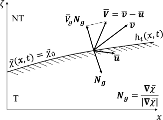
Figure 2: Definition sketch of the global (average) perspective on the turbulent-nonturbulent interface (TNTI).

3.2 Slender flows

Many free shear flows have the additional property of being slender, i.e. they develop much more slowly in the streamwise $x$-direction than in the normal direction, which implies that, apart from all quantities changing slowly in the $x$-direction, $\partial\overline{\chi}/\partial x\ll|\boldsymbol{\nabla}_{\perp}\overline{\chi}|$. Under the assumption of slenderness, (13), (15) become

$$\makebox[0.0pt]{$\phantom{V}\overline{\phantom{V}}$}V_{g}=-\frac{1}{|\boldsymbol{\nabla}_{\perp}\overline{\chi}|}\frac{\overline{D}\overline{\chi}}{\overline{D}t}=\overline{u}_{\zeta}-\frac{\overline{D}h_{t}}{\overline{D}t}.$$ (18)

The assumption of slenderness also implies that $|N_{gx}|\ll|\boldsymbol{N}_{g\perp}|$, which furthermore implies that $|\boldsymbol{N}_{g\perp}|\approx 1$ and $\boldsymbol{N}_{g\perp}\approx\boldsymbol{n}_{g}=\boldsymbol{\nabla}_{\perp}\overline{\chi}/|\boldsymbol{\nabla}_{\perp}\overline{\chi}|$. Thus, under this assumption the equations (16,17) further simplify to

$$\frac{\partial}{\partial t}{\int_{\overline{\Omega}}~{}\textnormal{d}A}+\frac{\partial}{\partial x}\int_{\overline{\Omega}}\overline{u}_{x}~{}\textnormal{d}A=-\oint_{\partial\overline{\Omega}}\makebox[0.0pt]{$\phantom{V}\overline{\phantom{V}}$}V_{g}~{}\textnormal{d}\ell,$$ (19)

$$\begin{split}\frac{\partial}{\partial t}\int_{\overline{\Omega}}\overline{u}_{x}~{}\textnormal{d}A&+\frac{\partial}{\partial x}\int_{\overline{\Omega}}\left(\overline{u_{x}^{2}}+\frac{\overline{p}}{\rho_{0}}\right)~{}\textnormal{d}A\\ &=-\oint_{\partial\overline{\Omega}}\left(\overline{V_{g}u_{x}}-\frac{\overline{p}}{\rho_{0}}N_{gx}\right)~{}\textnormal{d}\ell+\int_{\overline{\Omega}}\overline{f}_{x}\textnormal{d}A.\end{split}$$ (20)

4 Implications

4.1 Reconciliation of entrainment definitions

Equation (18) brings perspective to the different definitions of the global entrainment velocity that have previously been used. Taking the example of an axisymmetric jet, it follows that $\zeta=r$ and thus that (18) is given by

$$\makebox[0.0pt]{$\phantom{V}\overline{\phantom{V}}$}V_{g}(x,t)=\overline{u}_{r}(x,h_{t},t)-\left(\frac{\partial h_{t}}{\partial t}(x,t)+\overline{u}_{x}(x,h_{t},t)\frac{\partial h_{t}}{\partial x}(x,t)\right).$$ (21)

Hunt et al. (1983); Turner (1986), discuss the different definitions that were used in the thirty years prior, and distinguished between the entrainment rate $E$, a boundary entrainment rate $E_{b}$ and a net entrainment rate $E^{*}$. Loosely speaking, one can relate $\makebox[0.0pt]{$\phantom{V}\overline{\phantom{V}}$}V_{g}$ with the net entrainment rate $E^{*}$, $\overline{u}_{r}$ with the entrainment rate $E$ and $\overline{D}h_{t}/\overline{D}t$ with the boundary entrainment rate $E_{b}$, such that $E^{*}=E-E_{b}$. However, note that only steady problems were considered in these discussions. The definitions of $E^{*}$, $E$ and $E_{b}$ will be detailed below, as well as the similarities and differences in the concepts.

In Hunt et al. (1983); Turner (1986), $E$ and $E_{b}$ were determined from the top-hat ”cartoon” of a jet, i.e. the jet has a width $h$ with a uniform velocity $u_{m}$ inside and zero velocity outside it (this viewpoint has been used extensively for integral descriptions of free shear flows and should not be applied locally, e.g. to quantify Reynolds stresses which would be zero). Here, the top-hat width $h$ and velocity $u_{m}$ are defined as $h=Q/M^{1/2}$ and $u_{m}=M/Q$, where $Q=2\int_{0}^{h_{t}}\overline{u}_{x}r\textnormal{d}r$ is the volume flux and $M=2\int_{0}^{h_{t}}\overline{u}_{x}^{2}r\textnormal{d}r$ is the momentum flux per unit radian. For a steady jet, $\textnormal{d}h/\textnormal{d}x=2\alpha$, where $\alpha$ is the entrainment rate (Turner, 1986). In the cartoon view, $E=-\alpha u_{m}$ is the flow perpendicular through the jet boundary, and $E_{b}=u_{m}\textnormal{d}h/\textnormal{d}x$ is the outward velocity of an observer moving along the interface. Using the spreading rate of the jet, we can write this as $E_{b}=2\alpha u_{m}=2E$, such that the net entrainment rate $E^{*}=-3E$.

However, the classical arguments suggest that there is a choice in the entrainment definition when (21) clarifies there is not. Indeed, if we restrict ourselves to a steady flow and choose a conventional threshold strategy by using $\overline{\chi}=\overline{u}(x,r)/u_{m}(x)$ (e.g. van Reeuwijk et al., 2016), then we immediately obtain that

$$\makebox[0.0pt]{$\phantom{V}\overline{\phantom{V}}$}V_{g}(x,t)=\overline{u}_{r}(x,h_{t})-\underbrace{\overline{\chi}_{0}u_{m}\frac{\textnormal{d}h_{t}}{\textnormal{d}x}}_{\approx 0},$$ (22)

where the boundary contribution can be assumed zero because $\overline{\chi}_{0}\ll 1$. This then immediately implies that $E_{b}\approx 0$, and that the only correct expression for the entrainment rate for the steady axisymmetric jet is that $E^{*}=E$.

4.2 Relation between $h$ and $h_{t}$

Integral models do not typically make explicit reference to a scalar interface $h_{t}$. Instead, it is conventional to define a characteristic width of the flow $h$ from either integral flow properties, resulting in a (top-hat) width $h=Q/M^{1/2}$ (as used in the previous section), or via the specific features of a given velocity profile, such the half-width $h_{1/2}$, defined as $\overline{u}_{x}(x,h_{1/2})=\overline{u}_{x}(x,0)/2$ where $\overline{u}_{x}(x,0)$ and is the centreline velocity.

For self-similar flows, $h$ and $h_{1/2}$ and $h_{t}$ are trivially related by a proportionality coefficient which translates through to the value of the entrainment coefficient. Therefore, they play an influential, albeit superficial, role in studies of entrainment. A further complication arises in flows that are not self-similar, which makes it impossible to relate $h$ with $h_{t}$ using a constant of proportionality (see §5.4)

Note that $h_{t}$ is present in the definitions of the the volume flux $Q$ and momentum flux $M$. This is important from a practical perspective as the flow in the ambient, even if only considering the induced irrotational flow due to entrainment, will not necessarily produce a finite volume flux from integrals to infinity (Kotsovinos, 1978) and will contaminate the results.

4.3 Entrainment interacting with turbulence

Although turbulent entrainment is usually associated with a net velocity relative to an interface to the interior turbulence, it is important to acknowledge that in turbulent ambients there are also turbulent-turbulent exchanges across the interface. These are not present in the continuity equation, which does not contain products, but these terms do feature in the momentum and scalar equations. For example, in (20), the term $\overline{V_{g}u_{x}}=\makebox[0.0pt]{$\phantom{V}\overline{\phantom{V}}$}V_{g}\overline{u}_{x}+\overline{V_{g}^{\prime}u_{x}^{\prime}}$ contains two contributions, one associated with the mean flow and one with turbulent exchanges across the interface. These can be expected to be important in environments in which there are substantial fluctuations in the ambient, such as jets in a turbulent environment (Ching et al., 1995; Gaskin et al., 2004; Kankanwadi & Buxton, 2019), turbulent fountains (Hunt & Burridge, 2015) or clouds (de Rooy, 2013). Importantly, the turbulent transport $\overline{V_{g}^{\prime}u_{x}^{\prime}}$ may require different parameterisation than the mean transport $\makebox[0.0pt]{$\phantom{V}\overline{\phantom{V}}$}V_{g}\overline{u}_{x}$.

4.4 Connection between the local and global viewpoints

The integral representations of the local and global continuity equations, (11) and (16) respectively, can be used to establish the relation between the local entrainment velocity and the global entrainment velocity. If the threshold $\chi_{0}$ encompasses all of the turbulence and $\overline{\chi}_{0}$ accounts for the mean area of the turbulent region, the left-hand sides of (11) and (16) can be assumed to be approximately equal. This results in

$$\overline{\oint_{\partial\Omega}\frac{V_{n}}{|\boldsymbol{N}_{\perp}|}~{}\textnormal{d}\ell}=\oint_{\partial\overline{\Omega}}\frac{\makebox[0.0pt]{$\phantom{V}\overline{\phantom{V}}$}V_{g}}{|\boldsymbol{N}_{g\perp}|}~{}\textnormal{d}\ell.$$ (23)

Consistent with Zhou & Vassilicos (2017), we introduce the average instantaneous interface and average interface lengths as $\mathcal{L}=\overline{\oint_{\partial\Omega}\textnormal{d}\ell}$ and $\mathcal{L}_{g}=\oint_{\partial\overline{\Omega}}\textnormal{d}\ell$, respectively. Note that $\mathcal{L}_{g}$ can be determined straightforwardly from the problem geometry and $h_{t}$ (see also §5). The average instantaneous interface length ${\mathcal{L}}$ is expected to scale in a fractal manner (Sreenivasan et al., 1989), implying that $\mathcal{L}\gg\mathcal{L}_{g}$ for $Re\gg 1$. Equation (23) can be recast as (van Reeuwijk & Holzner, 2014; Zhou & Vassilicos, 2017)

$$\frac{\langle\makebox[0.0pt]{$\phantom{V}\overline{\phantom{V}}$}V_{g}\rangle}{\langle V_{n}\rangle}=\frac{\mathcal{L}}{\mathcal{L}_{g}},$$ (24)

where $\langle V_{n}\rangle=\mathcal{L}^{-1}\overline{\oint_{\partial\Omega}V_{n}/|\boldsymbol{N}_{\perp}|\textnormal{d}\ell}$ and $\langle\overline{V}_{g}\rangle={\mathcal{L}_{g}}^{-1}\oint_{\partial\overline{\Omega}}\makebox[0.0pt]{$\phantom{V}\overline{\phantom{V}}$}V_{g}/|\boldsymbol{N}_{g\perp}|\textnormal{d}\ell$ are the effective local and global entrainment velocity, respectively. The fractal arguments for $\mathcal{L}$ can imply that the local entrainment velocity $\langle V_{n}\rangle$ is of the order of the Kolmogorov velocity (Corrsin & Kistler, 1955; van Reeuwijk & Holzner, 2014; Silva et al., 2018) for a specific value of the fractal dimension of the interface, but Zhou & Vassilicos (2017) also argued for the possibility of a different scaling, independent of the value of the fractal dimension, in the presence of non-equilibrium turbulence. It must be noted, however, that the definition of local entrainment velocity used by Zhou & Vassilicos (2017) actually relates to a pseudo-velocity (see Appendix A and section B.2 of Appendix B). Even so, their local entrainment velocity does scale with the Kolmogorov velocity in the presence of classical equilibrium turbulence. The connection between local and global entrainment was shown to hold reasonably well for an experimental study of a developing boundary layer (Chauhan et al., 2014).

It is unlikely that (23) will hold in an exact manner as $\overline{\chi}_{0}\rightarrow 0$, since global entrainment implicitly accounts for fluid entering or leaving non-turbulent regions where $\chi_{0}<\overline{\chi}<\overline{\chi}_{0}$. Indeed, Burridge et al. (2017) found that about five percent of the volume flux of a plume occurs outside of the turbulent region. For flows which are spatially and temporally evolving, deviations will likely be higher. Nevertheless, (23) is useful from a conceptual and practical point of view, because global entrainment is relatively straightforward to compute.

5 Application to four canonical flows

In this section the integral description will be applied to four canonical free shear flows namely the axisymmetric jet, the planar wake, the temporal jet and the unsteady jet/plume. The first three cases serve to demonstrate that the framework reproduces the appropriate entrainment velocities and well-known equations and results. The fourth case, the unsteady jet/plume, will provide new insight into the interpretation of the entrainment coefficient $\alpha$. As turbulent free shear flows are characterised by a high Reynolds number Re and a slow development in the $x$ (or $t$) direction, viscous stresses and pressure are neglected. Furthermore, consistent with general practice on thresholding, all quantities containing a prefactor $\overline{\chi}_{0}$ will neglected.

5.1 Axisymmetric jet

The axisymmetric jet is homogeneous in the azimuthal direction $\theta$ and time $t$. The streamwise velocity $\overline{u}_{x}$ is used to define the turbulent region for the global entrainment as $\overline{\chi}=\overline{u}_{x}/u_{m}(x)$, where $u_{m}(x)$ is the characteristic velocity inside the jet. Applying the symmetries to (18) and setting $\zeta=r$, we have

$$\makebox[0.0pt]{$\phantom{V}\overline{\phantom{V}}$}V_{g}=\overline{u}_{r}(x,h_{t}).$$ (25)

Thus, (19), (20) are given by, using that $\textnormal{d}A=2\pi r\textnormal{d}r$ and $\mathcal{L}_{g}=2\pi h_{t}$:

$$2\frac{\textnormal{d}}{\textnormal{d}x}\int_{0}^{h_{t}}\overline{u}_{x}r\textnormal{d}r=-2h_{t}\makebox[0.0pt]{$\phantom{V}\overline{\phantom{V}}$}V_{g}=-2h_{t}\overline{u}_{r},$$ (26)

$$2\frac{\textnormal{d}}{\textnormal{d}x}\int_{0}^{h_{t}}\overline{u_{x}^{2}}~{}r\textnormal{d}r=0,$$ (27)

which is consistent with straightforward integration of the Reynolds-averaged boundary layer equations (e.g. Rajaratnam, 1976), thereby confirming the appropriateness of the description.

5.2 Planar wake

The planar wake is an interesting case, since it features a nonzero ambient flow of amplitude $U_{\infty}$. This problem is statistically homogeneous in $y$ and $t$. Applying the symmetries to (18), setting $\zeta=z$ and using $\overline{\chi}=1-\overline{u}_{x}/U_{\infty}$ as the quantity for thresholding, we obtain

$$\makebox[0.0pt]{$\phantom{V}\overline{\phantom{V}}$}V_{g}=\overline{u}_{z}-U_{\infty}\frac{\textnormal{d}h_{t}}{\textnormal{d}x}.$$ (28)

Using that $\textnormal{d}A=L_{y}\textnormal{d}z$ and $\mathcal{L}_{g}=2L_{y}$ (since the interface is present on both sides of the $z=0$ plane), (19) and (20) are given by

$$\frac{\textnormal{d}}{\textnormal{d}x}\int_{-h_{t}}^{h_{t}}\overline{u}_{x}\textnormal{d}z=-2\makebox[0.0pt]{$\phantom{V}\overline{\phantom{V}}$}V_{g}=2\left(U_{\infty}\frac{\textnormal{d}h_{t}}{\textnormal{d}x}-\overline{u}_{z}\right),$$ (29)

$$\begin{split}\frac{\textnormal{d}}{\textnormal{d}x}\int_{-h_{t}}^{h_{t}}\overline{u_{x}^{2}}~{}\textnormal{d}z&=2U_{\infty}\left(U_{\infty}\frac{\textnormal{d}h_{t}}{\textnormal{d}x}-\overline{u}_{z}\right).\\ \end{split}$$ (30)

By substituting (29) into (30), assuming that $\overline{u^{\prime}_{x}u^{\prime}_{x}}\ll\overline{u}_{x}^{2}$ and rearranging it follows that the mean momentum deficit $\int_{-h_{t}}^{h_{t}}\overline{u}_{x}(U_{\infty}-\overline{u}_{x})\textnormal{d}z$ is conserved as expected (e.g. Pope, 2000).

5.3 Temporal jet

The capability to directly quantify the entrainment velocity $\makebox[0.0pt]{$\phantom{V}\overline{\phantom{V}}$}V_{g}$ in temporal free shear flows (e.g. atmospheric boundary layers) is one of the useful results of the integral description put forward here. The distinguishing aspect of these flows is that they tend to be homogeneous in $x$ and $y$. For a temporal jet, in order to obtain an expression for the global entrainment velocity we can define a threshold $\overline{\chi}=\overline{u}_{x}/u_{m}(t)$, where $u_{m}(t)$ is the characteristic value inside the jet (van Reeuwijk & Holzner, 2014). Applying the symmetries of this flow to (18) then results in

$$\makebox[0.0pt]{$\phantom{V}\overline{\phantom{V}}$}V_{g}=-\frac{\textnormal{d}h_{t}}{\textnormal{d}t}.$$ (31)

Using that $\textnormal{d}A=L_{y}\textnormal{d}z$ and $\mathcal{L}_{g}=2L_{y}$, (19) and (20) simplify to

$$2L_{y}\frac{\textnormal{d}h_{t}}{\textnormal{d}t}=-2L_{y}\makebox[0.0pt]{$\phantom{V}\overline{\phantom{V}}$}V_{g}=2L_{y}\frac{\textnormal{d}h_{t}}{\textnormal{d}t},$$ (32)

$$\begin{split}L_{y}\frac{\textnormal{d}}{\textnormal{d}t}\int_{-h_{t}}^{h_{t}}\overline{u}_{x}~{}\textnormal{d}A&=0.\end{split}$$ (33)

The first equation simply confirms that $\makebox[0.0pt]{$\phantom{V}\overline{\phantom{V}}$}V_{g}$ has been defined appropriately, whilst the second equation demonstrates the conservation of volume flux for this flow (van Reeuwijk & Holzner, 2014).

The equivalence between the integrals of local and global entrainment (24), was studied in van Reeuwijk & Holzner (2014). It was shown that for the temporal jet, the entrainment at the global and local level are indeed identical over several decades of variation in $\chi_{0}$ (enstrophy in this case), provided it was small enough. However, for the relatively low Reynolds number under consideration it was shown to be important to take into account the change in the interface location upon changing the threshold value $\chi_{0}$ if one were to determine the entrainment coefficient $\alpha$ from the local entrainment velocity. The consistency between the integral global and local entrainment flux (24) was shown also for the case of penetrative convection (Holzner & van Reeuwijk, 2017) and an inclined temporal gravity current (van Reeuwijk et al., 2018).

5.4 Unsteady axisymmetric jets and plumes

In this section we apply the description to unsteady axisymmetric jets and plumes, which will provide new insight in the extent to which the entrainment coefficient $\alpha$ is linked to actual entrainment across the jet/plume boundary. Axisymmetric statistically unsteady jets and plumes retain a dependence on three independent variables: the streamwise direction $x$, the lateral or normal direction $r$, and time $t$. In the case of unsteady jets and plumes, it cannot be assumed that the flow remains slender, since there can be substantial variation of all the quantities of interest over short distances. As for the axisymmetric jet, the streamwise velocity $\overline{u}_{x}$ is used to define the turbulent region for the global entrainment as $\overline{\chi}=\overline{u}_{x}/u_{m}(x,t)$, where $u_{m}(x)$ is the characteristic velocity inside the jet. Applying the symmetries to (16), setting $\zeta=r$ and $\textnormal{d}A=2\pi r\textnormal{d}r$ we obtain

$$\frac{\partial h_{t}^{2}}{\partial t}+\frac{\partial Q}{\partial x}=-\frac{1}{\pi}\oint_{\partial\overline{\Omega}}\frac{\makebox[0.0pt]{$\phantom{V}\overline{\phantom{V}}$}V_{g}}{|\boldsymbol{N}_{g\perp}|}~{}\textnormal{d}\ell,\\$$ (34)

where $Q=2\int_{0}^{h_{t}}\overline{u}_{x}r\textnormal{d}r$. The right-hand side accords with our intuitive understanding of entrainment across a physically defined interface. Similarly, defining a specific momentum flux $M=2\int_{0}^{h_{t}}\overline{u}_{x}^{2}r\textnormal{d}r$, the integral or top-hat width $h=Q/\sqrt{M}$ of an unsteady jet or plume obeys (Craske & van Reeuwijk, 2016)

$$\frac{1}{\gamma}\frac{\partial h^{2}}{\partial t}+\frac{\partial Q}{\partial x}=2\alpha M^{1/2},$$ (35)

where $\alpha$ is an entrainment coefficient that depends on dimensionless properties of the flow, such as the Richardson number, dimensionless steamwise gradients and parameters characterising the flow’s radial dependence. The dimensionless parameter $\gamma$ characterises the shape of the mean velocity in the plume as an integral of the mean flux of streamwise kinetic energy divided by $M^{2}/Q$. If one assumes self-similarity by introducing a similarity variable $\eta=r/h$, it directly follows that 1) $h_{t}=\eta_{t}h$ where $\eta_{t}$ is a constant; and 2) that $\gamma$ is a constant (4/3 for a Gaussian profile). In this case, the terms in (34) and (35) can be matched individually with result

$$\eta_{t}=\gamma^{-1/2},\quad\quad\alpha=-\frac{1}{2\pi M^{1/2}}\oint_{\partial\overline{\Omega}}\frac{\makebox[0.0pt]{$\phantom{V}\overline{\phantom{V}}$}V_{g}}{|\boldsymbol{N}_{g\perp}|}~{}\textnormal{d}\ell\equiv\alpha_{0}.$$ (36)

Equation (36) shows that for an unsteady flow that remains self-similar, the global entrainment coefficient $\alpha$ represents physical entrainment across its boundary $h_{t}$, entirely consistent with its classical interpretation.

However, in the vicinity of abrupt changes in the streamwise direction, unsteady jets and plumes depart significantly from self-similarity (Craske & van Reeuwijk, 2015, 2016). In this case, the equivalence between the individual terms in (34) and (35) is lost. Consequently, the strongest statement that can be made regarding the entrainment coefficient is that

$$\alpha=\underbrace{-\frac{1}{2\pi\,M^{1/2}}\oint_{\partial\overline{\Omega}}\frac{\makebox[0.0pt]{$\phantom{V}\overline{\phantom{V}}$}V_{g}}{|\boldsymbol{N}_{g\perp}|}~{}\textnormal{d}\ell}_{\alpha_{0}}+\underbrace{\frac{1}{2M^{1/2}}\left(\frac{\partial}{\partial t}\left(\frac{h^{2}}{\gamma}-h_{t}^{2}\right)+\frac{h^{2}}{\gamma^{2}}\frac{\partial\gamma}{\partial t}\right)}_{\alpha_{1}}.$$ (37)

The entrainment coefficient $\alpha_{0}$ continues to account for fluid entrained across the TNTI and therefore has a direct physical interpretation. In contrast, the pseudo entrainment described by $\alpha_{1}$ reconciles the definition of $\alpha$, as stated in (35) terms of $Q$ and $M$, with entrainment across the TNTI during departures from self-similarity. It accounts for differences between temporal changes in the widths $h$ and $h_{t}$, in addition to temporal changes in the parameter $\gamma$, which accounts for a change in the shape of the mean velocity profile.

If, in view of such difficulties, one is tempted to suggest that we should abandon (35) and focus on (34) instead, it should be noted that (35), unlike (34), can be readily augmented with a conservation equation for momentum containing $\partial_{t}Q+\partial_{x}M$ to produce a tractable model (Craske & van Reeuwijk, 2016). Indeed, it is for this reason that establishing the connection between the local and global perspectives of entrainment is crucial.

6 Conclusions

Turbulent entrainment lies at the core of many important applications in engineering and science. This paper developed an integral description of turbulent free shear flows that develop in space and/or time. It connects local and global descriptions of turbulent entrainment, and provides a simple and clear notation to describe the intricacies of TNTI dynamics. The description relies on the relative velocity between the fluid and the scalar interface $V_{n}$. By applying this description, in which the interface is defined implicitly via the isosurface $\chi=\chi_{0}$, in a local manner, integral equations are obtained that explicity feature the role of local entrainment.

By using an average scalar field $\overline{\chi}$, an equation for the global entrainment velocity $\makebox[0.0pt]{$\phantom{V}\overline{\phantom{V}}$}V_{g}$ was obtained, which resulted in equation (15) formulated in terms of the interface thickness $h_{t}$. For slender flows, this equation simplified to $\makebox[0.0pt]{$\phantom{V}\overline{\phantom{V}}$}V_{g}=\overline{u}_{\zeta}-\overline{D}h_{t}/\overline{D}t$. The associated integral equations make a statement about global entrainment.

The description can be used to provide insight into the different entrainment mechanisms of canonical free shear flows. One important example where it can provide insight is the parameterisation of entrainment for plumes in crossflows. This flow is interesting since it will have significant contributions from both direct entrainment ($\overline{u}_{\zeta}$) and from the Leibniz terms (Schatzman, 1978; Davidson, 1986). A detailed investigation using direct numerical simulation is currently underway that investigates both types of entrainment. The method will also be of interest to studying entrainment in clouds (de Rooy, 2013). Furthermore, the description can be applied to turbulent boundary layers (Townsend, 1976; Chauhan et al., 2014) and their control (Gad-El-Hak & Bushnell, 1991), particularly in combination with recently developed decomposition techniques for local (Holzner & Luethi, 2011) and global (van Reeuwijk & Craske, 2015) descriptions of turbulent entrainment. The description can also be used to link entrainment to non-equilibruim turbulence (Zhou & Vassilicos, 2017; Cafiero & Vassilicos, 2019).

Identifying discrete events that are responsible for entrainment has been a major focus in entrainment research since its inception (e.g. Townsend, 1976; Fernando, 1991). The description in its current form is not directly able to link turbulent entrainment to local and discrete events, since the integrals sum over all events. However, it is possible to combine the entrainment descriptions to a method to identify coherent structures (e.g. Neamtu-Halic et al., 2020), although one should keep in mind that the choice of local or global entrainment description can isolate different aspects of entrainment (engulfing or nibbling, for example) which one can then link to each other via local-global approximate balances such as the one discussed in §4.4. It is hoped that the current description will be able to assist in connecting macro-scale to micro-scale entrainment events and processes.

Declaration of interests

The authors report no conflict of interest.

Appendix A Integral identities

In this appendix we derive the integral identities (5)-(7) by considering volume and time integrals over infinitesimal slices of size $\delta x\rightarrow 0$ and $\delta t\rightarrow 0$, respectively. The identity (5) for the integral gradient operator can be obtained directly from (6) by substituting $\boldsymbol{F}=\phi\boldsymbol{e}_{i}$ for $i\in\{x,y,z\}$; we therefore only need to prove (6) and (7). We start with the proof of (6) which is a generalisation of the method introduced by Zhou & Vassilicos (2017) in their Appendix. The first step is to decompose $\int_{\Omega}\boldsymbol{\nabla}\cdot\boldsymbol{F}\textnormal{d}A$ as follows:

$$\int_{\Omega}\boldsymbol{\nabla}\cdot\boldsymbol{F}\textnormal{d}A=\int_{\Omega}\frac{\partial F_{x}}{\partial x}\textnormal{d}A+\int_{\Omega}\boldsymbol{\nabla}\cdot_{\perp}\boldsymbol{F}_{\perp}\textnormal{d}A=\int_{\Omega}\frac{\partial F_{x}}{\partial x}\textnormal{d}A-\oint_{\partial\Omega}\boldsymbol{F}_{\perp}\cdot\boldsymbol{n}\textnormal{d}\ell,$$ (38)

where use is made of Gauss’s divergence theorem (cf. Stokes’ theorem in appendix B) in the $y-z$ plane and $\boldsymbol{n}=\boldsymbol{N}_{\perp}/|\boldsymbol{N}_{\perp}|=\boldsymbol{\nabla}_{\perp}\chi/|\boldsymbol{\nabla}_{\perp}\chi|$ is the surface normal in the $y-z$ plane. Note that the minus sign in the last term of (38) originates from the fact that $\boldsymbol{n}$ points into $\Omega$ rather than outwards.

We now seek a formula for commuting $\int_{\Omega}$ and $\partial/\partial x$ in (38). Note that

$$\begin{split}\frac{\partial}{\partial x}\int_{\Omega}F_{x}\textnormal{d}A=\lim_{\delta x\to 0}\frac{1}{\delta x}\left(\int_{\Omega(x+\delta x)}F_{x}(x+\delta x)\textnormal{d}A-\int_{\Omega(x)}F_{x}(x)\textnormal{d}A\right)\\ =\int_{\Omega(x)}\frac{\partial F_{x}}{\partial x}\textnormal{d}A+\lim_{\delta x\to 0}\frac{1}{\delta x}\left[\int_{\Omega(x+\delta x)}F_{x}(x+\delta x)\textnormal{d}A-\int_{\Omega(x)}F_{x}(x+\delta x)\textnormal{d}A\right].\end{split}$$ (39)

The bracketed term in (39) is the difference between the surface integrals of $F_{x}(x+\delta x)$ over $\Omega(x+\delta x)$ and over $\Omega(x)$ respectively. This integral is crucially related to the slope of the interface with the $x-$direction, $N_{x}/|\boldsymbol{N}_{\perp}|$. Indeed, the amount of substance flowing into $\Omega$ at a certain location on the interface due to the slope is equal to $F_{x}\delta h_{t}\delta\ell$, where $\delta h_{t}$ is the change in the interface position in the $y-z$ plane (normal to $\delta\ell$) over the streamwise distance $\delta x$. Since $\delta h_{t}=N_{x}/|\boldsymbol{N}_{\perp}|\delta x$ (Figure 1b), it follows that the difference between the two surface integrals is, to leading order, equal to the curvilinear integral $\oint_{\partial\Omega}F_{x}(x+\delta x)N_{x}/|\boldsymbol{N}_{\perp}|\delta x\textnormal{d}\ell$. Hence, (39) becomes

$$\frac{\partial}{\partial x}\int_{\Omega}F_{x}\textnormal{d}A=\int_{\Omega}\frac{\partial F_{x}}{\partial x}\textnormal{d}A+\oint_{\partial\Omega}F_{x}\frac{N_{x}}{|\boldsymbol{N}_{\perp}|}\textnormal{d}\ell.$$ (40)

Combining (40) with (38) leaves us with our first main general result, identity (6).

In the case where $\boldsymbol{F}=Q\boldsymbol{u}$ for some field $Q$, we have $F_{x}(x){N_{x}}/{|\boldsymbol{N}_{\perp}|}=Q(x)u_{x}(x){N_{x}}/{|\boldsymbol{N}_{\perp}|}$. Defining $\textnormal{d}t$ to be the time required for a fluid element to move a distance $\textnormal{d}x=u_{x}\textnormal{d}t$ in the streamwise direction, Zhou & Vassilicos (2017) defined the pseudo-velocity ${\textnormal{d}h_{t}}/{\textnormal{d}t}$ which they termed $V_{n}$ (not to be confused with the definition of $V_{n}$ in the present paper). Given that their $V_{n}$ equals $u_{x}(x){N_{x}}/{|\boldsymbol{N}_{\perp}|}$, $\oint_{\partial\Omega}F_{x}(x){N_{x}}/{|\boldsymbol{N}_{\perp}|}\textnormal{d}\ell=\oint_{\partial\Omega}Q(x)V_{n}{N_{x}}/{|\boldsymbol{N}_{\perp}|}\textnormal{d}\ell$ in terms of their pseudo-velocity $V_{n}$ (see also section B.2 of Appendix B). This establishes the correspondence between the results in their Appendix (which they gave for $Q=1$) and (40), (6) here.

We now proceed with the proof of identity (7). Integrating the material derivative over $\Omega$ yields

$$\int_{\Omega}\frac{D\phi}{Dt}\textnormal{d}A=\int_{\Omega}\frac{\partial}{\partial t}\phi~{}\textnormal{d}A+\int_{\Omega}\boldsymbol{\nabla}\cdot(\phi\boldsymbol{u})~{}\textnormal{d}A-\int_{\Omega}\phi\boldsymbol{\nabla}\cdot\boldsymbol{u}\textnormal{d}A$$ (41)

and then making use of (6) for $\boldsymbol{F}=\phi\boldsymbol{u}$,

$$\int_{\Omega}\frac{D\phi}{Dt}\textnormal{d}A=\int_{\Omega}\frac{\partial}{\partial t}\phi~{}\textnormal{d}A+\frac{\partial}{\partial x}\int_{\Omega}\phi u_{x}\textnormal{d}A-\oint_{\partial\Omega}\phi\boldsymbol{u}\cdot\frac{\boldsymbol{N}}{|\boldsymbol{N}_{\perp}|}\textnormal{d}\ell-\int_{\Omega}\phi\boldsymbol{\nabla}\cdot\boldsymbol{u}\textnormal{d}A.$$ (42)

Following (39), we now wish to commute $\int_{\Omega}$ and $\partial/\partial t$:

$$\begin{split}\frac{\partial}{\partial t}\int_{\Omega}\phi\textnormal{d}A=\lim_{\delta t\to 0}\frac{1}{\delta t}\left(\int_{\Omega(t+\delta t)}\phi(t+\delta t)\textnormal{d}A-\int_{\Omega(t)}\phi(t)\textnormal{d}A\right)\\ =\int_{\Omega(t)}\frac{\partial\phi}{\partial t}\textnormal{d}A+\lim_{\delta t\to 0}\frac{1}{\delta t}\left[\int_{\Omega(t+\delta t)}\phi(t+\delta t)\textnormal{d}A-\int_{\Omega(t)}\phi(t+\delta t)\textnormal{d}A\right].\end{split}$$ (43)

The bracketed term in (43) is the difference between the surface integrals of $\phi(t+\delta t)$ over $\Omega(t+\delta t)$ and over $\Omega(t)$ respectively. The interface, which moves at normal velocity $v_{n}=\boldsymbol{v}\cdot\boldsymbol{N}$, will move at velocity $v_{n}/|\boldsymbol{N}_{\perp}|$ when projected onto the $y-z$ plane. Thus, over a time increment $\delta t$, the interface element of length $\delta\ell$ will sweep an area in the $y-z$ plane equal to $-v_{n}/|\boldsymbol{N}_{\perp}|\delta t\delta\ell$ (the minus sign once more originates from the inward pointing normal $\boldsymbol{N}$). This implies that difference between the two surface integrals in (43) is, to leading order, equal to the curvilinear integral $-\oint_{\partial\Omega}\phi(t+\delta t)v_{n}/|\boldsymbol{N}_{\perp}|\delta t\textnormal{d}\ell$. Hence, (43) becomes

$$\frac{\partial}{\partial t}\int_{\Omega}\phi\textnormal{d}A=\int_{\Omega}\frac{\partial\phi}{\partial t}\textnormal{d}A-\oint_{\partial\Omega}\phi\frac{v_{n}}{|\boldsymbol{N}_{\perp}|}\textnormal{d}{\ell}.$$ (44)

Combining (44) with (42) and invoking the relative iso-surface velocity $\boldsymbol{V}=\boldsymbol{v}-\boldsymbol{u}$, leaves us with our second main general result, identity (7), i.e.

$$\int_{\Omega}\frac{D\phi}{Dt}\textnormal{d}A=\frac{\partial}{\partial t}\int_{\Omega}\phi~{}\textnormal{d}A+\frac{\partial}{\partial x}\int_{\Omega}u_{x}\phi~{}\textnormal{d}A+\oint_{\partial\Omega}\frac{V_{n}}{|\boldsymbol{N}_{\perp}|}\phi~{}\textnormal{d}\ell-\int_{\Omega}\phi\boldsymbol{\nabla}\cdot\boldsymbol{u}\textnormal{d}A.$$

Noting that the approaches used in (39) and (43) are equivalent and account for the commutation of integration with differentiation with respect to either time or space, we abstract and generalise our results using differential geometry in the following section.

Appendix B Differential geometry

In this appendix we regard the region $\Omega$, defined by an isosurface of $\chi$, as a submanifold whose shape changes as a function of codimensions $x$ and $t$, for example. In manipulating integrals of partial derivatives over $\Omega$, one is faced with two distinct types of expression. The first involves derivatives in directions that lie within the dimensions of $\Omega$ and the second involves derivatives in directions that lie in the codimension of $\Omega$. The first can be manipulated using a generalised version of Stokes’ theorem, whilst the second require a generalised form of Leibniz’s rule for commuting integration and partial differentiation. The first involve physical fluxes and velocities at the boundary $\partial\Omega$. The second, in contrast, involve pseudo fluxes and velocities that account for deformations of the integration domain with respect to changes in a given codimension. Since the integration domain is specified by $\chi$ independently of physical boundary fluxes, the two are independent.

To crystallise these ideas, consider an $n-$dimensional slice $\Omega$ through an $N-$dimensional manifold defined by $\chi(\boldsymbol{x},\boldsymbol{y})\geq\chi_{0}$ by fixing $m=N-n$ codimensions $\boldsymbol{x}$, as depicted in figure 3. The slice itself can be traversed locally by coordinates $y^{1},\ldots,y^{n}$. Components of a differential $(N-1)$-form $\omega$ can be partitioned into fluxes $f$ and $g$ that are either normal or tangential to the area form $\textnormal{d}A=\textnormal{d}y^{1}\wedge\textnormal{d}y^{2}\wedge\ldots\wedge\textnormal{d}y^{n}$, respectively. For example, if $x^{1}=x$, $y^{1}=y$ and $y^{2}=z$, a flux $\omega$ can be partitioned, such that:

$$\omega=\underbrace{\omega_{x}\textnormal{d}y\wedge\textnormal{d}z}_{f}+\underbrace{\omega_{y}\textnormal{d}z\wedge\textnormal{d}x+\omega_{z}\textnormal{d}x\wedge\textnormal{d}y}_{g}.$$ (45)

Integrals of the $N$-form $\textnormal{d}g$ at a given point in the codomain can be evaluated using a generalised version of the fundamental theorem of calculus in the form of Stokes’ theorem. With slight abuse of notation, because $\textnormal{d}g$ is an $N$-form rather than an $n$-form, we express the application of Stokes’ theorem over the slice $\Omega$ as

$$\int_{\Omega}\mathrm{d}g=\int_{\partial\Omega}g,$$ (46)

which we will refer to as a partial integral (Whitney, 2005) that results in a differential form containing, in the case of (46), $\textnormal{d}x^{1}\wedge\ldots\wedge\textnormal{d}x^{m}$. A more rigorous treatment of the operation would consider integrals along a fibre ($\Omega$) of a fibre bundle (the entire space). In either case, equation (46) states that integrals of derivatives with respect to $y^{1}\,\ldots,y^{n}$ can be evaluated as surface integrals that account for boundary transport.

The manipulation $\textnormal{d}f$ is fundamentally different from $\textnormal{d}g$ because $\textnormal{d}f$, unlike $\textnormal{d}g$, involves partial derivatives with respect to the codimensions $x^{1},\ldots,x^{m}$. Consequently, partial integrals of $\textnormal{d}f$ over $\Omega$ satisfy a generalised version of Leibniz’s rule that specifies how to commute integration with exterior differentiation:

$$\int_{\Omega}\textnormal{d}f=\textnormal{d}\int_{\Omega}f-\int_{\partial\Omega}h,$$ (47)

in which the partial integral of $f$ over $\Omega$ produces an $(m-1)$-form to which the exterior derivative $\mathrm{d}$ can be applied. The final term in (47) contains $h$, which is a differential $(N-1)$-form corresponding to a pseudo flux, in contrast with the physical flux $g$. The pseudo flux $h$ results from $f$ and the dependence of $\Omega$ on the codimensions, and therefore depends on the geometry of the surface $\chi-\chi_{0}=0$.

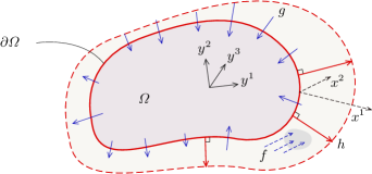
Figure 3: A submanifold $\Omega$ described by local coordinates $y^{1},\ldots,y^{n}$ and parameterised over codimensions $x^{1},\ldots,x^{m}$. The physical flux in the plane of $\Omega$ corresponds to the $(m+n-1)$-form $g$ and the pseudo flux, arising from the normal flux $f$ through deformations in $\partial\Omega$ as one moves with unit ‘velocity’ in the direction $x^{i}$ corresponds to the $(m+n-1)$-form $h$.

To determine $h$, we define a vector $Y$ that is tangent to $\Omega$, is perpendicular to an isosurface of $\chi$:

$$(\boldsymbol{\nabla}\chi\mathbin{\raisebox{0.0pt}{\scalebox{1.0}[-1.0]{$\lnot$}}}\textnormal{d}A)(Y)=0,$$ (48)

and corresponds to a unit rate of change down $\chi$, such that $\textnormal{d}\chi(Y)=-1$. Consequently, the vector $(\partial_{x^{i}}\chi)Y$ acts in a direction that is perpendicular to $\partial\Omega$ and describes the change in $\partial\Omega$ that occurs as one moves with unit ‘velocity’ along the $i^{\mathrm{th}}$ codimension. The effect of changes in $\Omega$ on integrals is captured by Cartan’s magic formula for the Lie derivative $X\mathbin{\raisebox{0.0pt}{\scalebox{1.0}[-1.0]{$\lnot$}}}\textnormal{d}\omega=\mathcal{L}_{X}\omega-\textnormal{d}(X\mathbin{\raisebox{0.0pt}{\scalebox{1.0}[-1.0]{$\lnot$}}}\omega)$, where $\mathcal{L}_{X}\omega$ describes the change in $\omega$ along the flow defined by $X$. Setting $X=\partial_{x^{i}}+(\partial_{x^{i}}\chi)Y$ and focusing on each component $f_{i}$ of $f$ in (45), leads to a generalised version of Leibniz’s rule (see, for example, Flanders, 1973) for partial integration over $\Omega$:

$$\int_{\Omega}\frac{\partial}{\partial x^{i}}\mathbin{\raisebox{0.0pt}{\scalebox{1.0}[-1.0]{$\lnot$}}}\textnormal{d}f_{i}=\frac{\partial}{\partial x^{i}}\int_{\Omega}f_{i}-\int_{\partial\Omega}\frac{\partial\chi}{\partial x^{i}}Y\mathbin{\raisebox{0.0pt}{\scalebox{1.0}[-1.0]{$\lnot$}}}f_{i},$$ (49)

which is an $(m-1)$-form. Applying $\textnormal{d}x^{i}\wedge$ to (49), and summing over each codimension $i$, shows that each term in (49) corresponds to the respective terms in (47) and therefore reveals that

$$h=Y\mathbin{\raisebox{0.0pt}{\scalebox{1.0}[-1.0]{$\lnot$}}}(\textnormal{d}\chi\wedge f),$$ (50)

which is fundamental in determining the boundary contribution of fluxes that are perpendicular to $\textnormal{d}A$. Combining (50) with (46) and (47) leads to a general formula for commuting exterior differentiation and partial integration over a submanifold:

$$\int_{\Omega}\textnormal{d}\omega-\textnormal{d}\int_{\Omega}\omega=\underbrace{\int_{\partial{\Omega}}g}_{\text{Stokes}}-\underbrace{\int_{\partial\Omega}h}_{\text{Leibniz}}.$$ (51)

As illustrated in figure 3, the commutation of integration and exterior differentiation leads to physical fluxes $g$ in the plane of $\textnormal{d}A$ in addition to pseudo fluxes $h$, which account for the flow $f$ through the contraction and expansion of $\Omega$ as the codimensions $t$ and $x$ change.

B.1 Example: integration of $D\phi/Dt$ over $\Omega(x,t)\ni(y,z)$

To integrate $D\phi/Dt$ over an area $\Omega(x,t)$, we identify $x^{1}=t$, $x^{2}=x$ as the submanifold’s codimensions and $y^{1}=y$, $y^{2}=z$ as the submanifold’s coordinates. We decompose $D\phi/Dt$ to incorporate the divergence of a flux $\omega$ and indicate the correspondance with $\textnormal{d}\omega=\textnormal{d}f+\textnormal{d}g$:

$$\frac{D\phi}{Dt}=\underbrace{\frac{\partial\phi}{\partial t}+\frac{\partial u_{x}\phi}{\partial x}}_{\textnormal{d}f}+\underbrace{\frac{\partial u_{y}\phi}{\partial y}+\frac{\partial u_{z}\phi}{\partial z}}_{\textnormal{d}g}-\phi\boldsymbol{\nabla}\cdot\boldsymbol{u},$$ (52)

which, regarding $D\phi/Dt$ as a differential 4-form, implies that

$$\omega=\underbrace{\phi\,\textnormal{d}x\wedge\textnormal{d}y\wedge\textnormal{d}z-u_{x}\phi\,\textnormal{d}t\wedge\textnormal{d}y\wedge\textnormal{d}z}_{f}+\underbrace{u_{y}\phi\,\textnormal{d}t\wedge\textnormal{d}x\wedge\textnormal{d}z-u_{z}\phi\,\textnormal{d}t\wedge\textnormal{d}x\wedge\textnormal{d}y}_{g}.$$ (53)

Here, the tangent vector $Y$ is:

$$Y=Y_{y}\frac{\partial}{\partial y}+Y_{z}\frac{\partial}{\partial z}=-\left(\left(\frac{\partial\chi}{\partial y}\right)^{2}+\left(\frac{\partial\chi}{\partial z}\right)^{2}\right)^{-1}\left(\frac{\partial\chi}{\partial y}\frac{\partial}{\partial y}+\frac{\partial\chi}{\partial z}\frac{\partial}{\partial z}\right),$$ (54)

which, using (51) and omitting the $\textnormal{d}t\wedge\textnormal{d}x$ that remains after partial integration, results in

$$\begin{split}\int_{\Omega}\frac{D\phi}{Dt}\textnormal{d}A=\frac{\partial}{\partial t}&\int_{\Omega}\phi\textnormal{d}A+\frac{\partial}{\partial x}\int_{\Omega}u_{x}\phi\textnormal{d}A+\int_{\partial\Omega}\left(Y_{z}\frac{\partial\chi}{\partial t}+u_{x}Y_{z}\frac{\partial\chi}{\partial x}-u_{z}\right)\phi\textnormal{d}y\\ &-\int_{\partial\Omega}\left(Y_{y}\frac{\partial\chi}{\partial t}+u_{x}Y_{y}\frac{\partial\chi}{\partial x}-u_{y}\right)\phi\textnormal{d}z-\int_{\Omega}\phi\boldsymbol{\nabla}\cdot\boldsymbol{u}\textnormal{d}A.\end{split}$$ (55)

Identities for the integral of $\boldsymbol{\nabla}\phi$ and the area of $\Omega$ can be obtained as corollaries of (55) by substitution of $\boldsymbol{u}=(1,1,1)^{T}$ and $\phi=1$, respectively.

B.2 Summary and connection with appendix A

Our results indicate that the commutation of integration and differentiation leads to storage terms and pseudo boundary fluxes that depend on the $t$ and $x$ dependence of the domain of integration. Such fluxes are distinct from the physical boundary fluxes that are obtained by applying Stokes’ theorem to the divergence of fluxes that are in the same plane as the domain of integration.

To link (51) with appendix A it is necessary to note that the vector $Y$ introduced at (48), and written explicitly in (54), corresponds to $-\boldsymbol{n}/|\boldsymbol{\nabla}_{\perp}\chi|$ and that

$$\frac{\partial\chi}{\partial t}=-v_{n}|\boldsymbol{\nabla}\chi|,\quad\quad\frac{\partial\chi}{\partial x}=u_{x}N_{x}|\boldsymbol{\nabla}\chi|.$$ (56)

As made explicit in the fourth term of (55), each term in the integral of $h$ accounts for $Y$, which is normal to $\partial\Omega$ according to (48), scaled by either $\partial_{t}\chi$ or $\partial_{x}\chi$. Consequently, by expanding (7) for $\phi=1$, using (56) and recalling that $|\boldsymbol{N}_{\perp}|=|\boldsymbol{\nabla}_{\perp}\chi|/|\boldsymbol{\nabla}\chi|$,

$$\frac{\partial}{\partial t}\int_{\Omega}\textnormal{d}A+\frac{\partial}{\partial x}\int_{\Omega}u_{x}\textnormal{d}A=\oint_{\partial\Omega}\underbrace{\boldsymbol{u}\cdot\boldsymbol{n}\textnormal{d}\ell}_{-g}-\oint_{\partial\Omega}\underbrace{\frac{v_{n}}{|\boldsymbol{N}_{\perp}|}-u_{x}\frac{N_{x}}{|\boldsymbol{N}_{\perp}|}\textnormal{d}\ell}_{-h},$$ (57)

which is a special case of the relation (51). The inward boundary flux $g=\boldsymbol{u}\cdot\boldsymbol{n}\textnormal{d}\ell$ results from Stokes’ theorem and is identical to $V_{f}\textnormal{d}\ell$ in Zhou & Vassilicos (2017). In contrast, the pseudo fluxes $h$ result from Leibniz’s rule for commuting integration and differentiation. The terms in $h$ correspond to perpendicular fluxes through contractions and expansions of the boundary $\partial\Omega$ as one traverses the codimensions $t$ and $x$ with unit velocity (see figure 3). Specifically, the term $u_{x}N_{x}/|\boldsymbol{N}_{\perp}|\textnormal{d}\ell$ corresponds to the increase in volume flux due to changes in the location of $\partial\Omega$ as one moves, one unit in the $x$ direction and is identical to $V_{n}\textnormal{d}\ell$ in Zhou & Vassilicos (2017) (stressing, again, that this $V_{n}$ is not the same as the $V_{n}$ defined in the present paper).

A practical advantage of the abstract approach adopted in appendix B is that the resulting surface integrals (see (55), for example) are given explicitly in terms of coordinate differentials $\textnormal{d}y$, $\textnormal{d}z$. The integral expressions can therefore be readily evaluated on a numerical grid and, since differential forms $\textnormal{d}y$, $\textnormal{d}z$, $\textnormal{d}y\wedge\textnormal{d}z$ have an orientation, automatically account for the orientation of a surface and its normal.

References

- Bisset et al. (2002) Bisset, D. K., Hunt, J. C. R. & Rogers, M. M. 2002 The turbulent/non-turbulent interface bounding a far wake. J. Fluid Mech. 451, 383–410.
- Burridge et al. (2017) Burridge, H. C., Parker, D. A., Kruger, E. S., Partridge, J. L. & Linden, P. F. 2017 Conditional sampling of a high Péclet number turbulent plume and the implications for entrainment. J. Fluid Mech. 823, 26–56.
- Cafiero & Vassilicos (2019) Cafiero, G. & Vassilicos, J.C. 2019 Non-equilibrium turbulence scalings and self-similarity in turbulent planar jets. Proc. R. Soc. Lond. A 475, 20190038.
- Cantwell & Coles (1983) Cantwell, B. & Coles, D. 1983 An experimental study of entrainment and transport in the turbulent near wake of a circular cylinder. J. Fluid Mech. 136, 321–374.
- Chauhan et al. (2014) Chauhan, K., Philip, J., de Silva, C. M., Hutchins, N. & Marusic, I. 2014 The turbulent/non-turbulent interface and entrainment in a boundary layer. J. Fluid Mech. 742, 119–151.
- Ching et al. (1995) Ching, C.Y., Fernando, H.J.S. & Robles, A. 1995 Break-down of line plumes in turbulent environments. Journal of Geophysical Research: Oceans 100, 4707–4713.
- Corrsin & Kistler (1955) Corrsin, S. & Kistler, A.L 1955 Free stream boundaries of turbulent flows. Tech. Rep. 1244. NACA.
- Craske & van Reeuwijk (2015) Craske, J. & van Reeuwijk, M. 2015 Energy dispersion in turbulent jets. Part 1. Direct simulation of steady and unsteady jets. J. Fluid Mech. 763, 500–537.
- Craske & van Reeuwijk (2016) Craske, J. & van Reeuwijk, M. 2016 Generalised unsteady plume theory. J. Fluid Mech. 792, 1013–1052.
- Da Silva et al. (2014) Da Silva, C. B., Hunt, J. C. R., Eames, I. & Westerweel, J. 2014 Interfacial layers between regions of different turbulence intensity. Annu. Rev. Fluid Mech. 46, 567–590.
- Da Silva & Métais (2002) Da Silva, C. B. & Métais, O. 2002 On the influence of coherent structures upon interscale interactions in turbulent plane jets. J. Fluid Mech. 473, 103–145.
- Da Silva & Pereira (2008) Da Silva, C. B. & Pereira, J. C. F. 2008 Invariants of the velocity-gradient, rate-of-strain, and rate-of-rotation tensors across the turbulent/nonturbulent interface in jets. Phys. Fluids 20 (5), 055101.
- Davidson (1986) Davidson, G.A. 1986 A discussion of Schatzmann’s integral plume nodel from a control volume viewpoint. J. Clim. Appl. Met. 25, 858–866.
- De Wit et al. (2014) De Wit, L., Van Rhee, C. & Keetels, G. 2014 Turbulent interaction of a buoyant jet with cross-flow. J. Hydr. Eng. 140 (12), 04014060.
- Deardorff et al. (1980) Deardorff, J. W., Willis, G. E. & Stockton, B. H. 1980 Laboratory studies of the entrainment zone of a convectively mixed layer. J. Fluid Mech. 100, 41–64.
- Devenish et al. (2010) Devenish, B.J., Rooney, G.G. & Thomson, D.J. 2010 Large-eddy simulation of a buoyant plume in uniform and stably stratified environments. J. Fluid Mech. 652, 75 – 103.
- Dopazo et al. (2007) Dopazo, C., Martín, J. & Hierro, J. 2007 Local geometry of isoscalar surfaces. Physical Review E 76 (5), 056316.
- Fernando (1991) Fernando, H. J. S. 1991 Turbulent mixing in stratified fluids. Annu. Rev. Fluid Mech. 23, 455–493.
- Flanders (1973) Flanders, Harley 1973 Differentiation under the integral sign. American Math. Monthly 80 (6), 615–627.
- Gad-El-Hak & Bushnell (1991) Gad-El-Hak, M. & Bushnell, D. M. 1991 Separation control: review. Journal of Fluids Engineering 115, 5–30.
- Garcia & Mellado (2014) Garcia, J.R. & Mellado, J.P. 2014 The two-layer structure of the entrainment zone in the convective boundary layer. J. Atmos. Sci. 71, 1935–1955.
- Gaskin et al. (2004) Gaskin, S.J., McKernan, M. & Xue, F. 2004 The effect of background turbulence on jet entrainment: an experimental study of a plane jet in a shallow coflow. Journalof Hydraulic Research 42 (5), 533–542.
- Head (1958) Head, M.R. 1958 Entrainment in the turbulent boundary layer. Reports & Memoranda 3152. Ministry of Aviation.
- Holzner & Luethi (2011) Holzner, M. & Luethi, B. 2011 Laminar superlayer at the turbulence boundary. Phys. Rev. Lett. 106 (13), 134503.
- Holzner & van Reeuwijk (2017) Holzner, M. & van Reeuwijk, M. 2017 The turbulent/nonturbulent interface in penetrative convection. J. Turbul. 18, 260–270.
- Hunt & Burridge (2015) Hunt, G.R. & Burridge, H.C. 2015 Fountains in industry and nature. Annu. Rev. Fluid Mech. 47, 195–220.
- Hunt et al. (1983) Hunt, J. C. R., Rottman, J.W. & Britter, R.E. 1983 Some physical processes involved in the dispersion of dense gases. In Proc. UITAM Symp. on Atmospheric dispersion of heavy gases and small particles (ed. G. Ooms & H. Tennekes), pp. 361–395. Springer.
- Hussein et al. (1994) Hussein, H. J., Capp, S. P. & George, W. K. 1994 Velocity measurements in a high-Reynolds number, momentum-conserving, axisymmetric, turbulent jet. J. Fluid Mech. 258, 31–75.
- Jahanbakhshi & Madnia (2018) Jahanbakhshi, R. & Madnia, C. 2018 The effect of heat release on the entrainment in a turbulent mixing layer. J. Fluid Mech. 844.
- Jonker et al. (2013) Jonker, H.J.J., Van Reeuwijk, M., Sullivan, P. & Patton, E. 2013 On the scaling of shear-driven entrainment: A DNS study. J Fluid Mech. 732, 150–165.
- Kankanwadi & Buxton (2019) Kankanwadi, K. & Buxton, O. 2019 Turbulent entrainment from a turbulent background. In Eleventh International Symposium on Turbulence and Shear Flow Phenomena.
- Kato & Phillips (1969) Kato, H. & Phillips, O. M. 1969 On the penetration of a turbulent layer into stratified fluid. J. Fluid Mech. 37, 643–655.
- Kotsovinos (1978) Kotsovinos, N. E. 1978 A note on the conservation of the volume flux in free turbulence. J. Fluid Mech. 86, 201–203.
- Krug et al. (2017) Krug, D., Chung, D., Philip, J. & Marusic, I. 2017 Global and local aspects of entrainment in temporal plumes. J. Fluid Mech. 812, 222–250.
- Krug et al. (2015) Krug, D., Holzner, M., Luethi, B., Wolf, M., Kinzelbach, W. & Tsinober, A. 2015 The turbulent/non-turbulent interface in an inclined dense gravity current. J. Fluid Mech. 765, 303–324.
- List (1982) List, E. J. 1982 Turbulent jets and plumes. Annu. Rev. Fluid Mech. 14 (1), 189–212.
- Mahesh (2013) Mahesh, K. 2013 The interaction of jets with cross-flow. Annu. Rev. Fluid Mech. 45, 379–407.
- Mellado (2012) Mellado, JP. 2012 Direct numerical simulation of free convection over a heated plate. J Fluid Mech. 712, 418–450.
- Mellado (2017) Mellado, J. P. 2017 Cloud-top entrainment in stratocumulus clouds. Annu. Rev. Fluid Mech. 49 (1), 145–169.
- Neamtu-Halic et al. (2020) Neamtu-Halic, M. M., Krug, D., Mollicone, J.P., van Reeuwijk, M., Haller, G. & Holzner, M. 2020 Connecting the time evolution of the turbulence interface to coherent structures. Journal of Fluid Mechanics 898, A3.
- Obligado et al. (2016) Obligado, M., Dairay, T. & Vassilicos, J. C. 2016 Nonequilibrium scalings of turbulent wakes. Phys. Rev. Fluids 1 (4), 044409.
- Odier et al. (2014) Odier, P., Chen, J. & Ecke, R. E. 2014 Entrainment and mixing in a laboratory model of oceanic overflow. J. Fluid Mech. 746, 498–535.
- Philip et al. (2014) Philip, J., Meneveau, C., de Silva, C. M. & Marusic, I. 2014 Multiscale analysis of fluxes at the turbulent/non-turbulent interface in high Reynolds number boundary layers. Phys. Fluids 26, 015105.
- Pope (2000) Pope, S. B. 2000 Turbulent flows. Cambridge University Press.
- Rajaratnam (1976) Rajaratnam, N. 1976 Turbulent Jets. Developments in Water Science 5. Elsevier.
- Redford et al. (2012) Redford, J. A., Castro, I. P. & Coleman, G. N. 2012 On the universality of turbulent axisymmetric wakes. J. Fluid Mech. 710, 419–452.
- van Reeuwijk & Craske (2015) van Reeuwijk, M. & Craske, J. 2015 Energy-consistent entrainment relations for jets and plumes. J. Fluid Mech. 782, 333 – 355.
- van Reeuwijk & Holzner (2014) van Reeuwijk, M. & Holzner, M. 2014 The turbulence boundary of a temporal jet. J. Fluid Mech. 739, 254–275.
- van Reeuwijk et al. (2019) van Reeuwijk, M., Holzner, M. & Caulfield, C. P. 2019 Mixing and entrainment are suppressed in inclined gravity currents. J. Fluid Mech. 873, 786–815.
- van Reeuwijk et al. (2018) van Reeuwijk, M., Krug, D. & Holzner, M. 2018 Small-scale entrainment in inclined gravity currents. Environ. Fluid Mech. 18 (1), 225–239.
- van Reeuwijk et al. (2016) van Reeuwijk, Maarten, Salizzoni, Pietro, Hunt, Gary R. & Craske, John 2016 Turbulent transport and entrainment in jets and plumes: A dns study. Phys. Rev. Fluids 1, 074301.
- de Rooy (2013) de Rooy, W.C. et al. 2013 Entrainment and detrainment in cumulus convection: an overview. Quart. J. Roy. Meteor. Soc. 139 (670), 1–19.
- Scase et al. (2006) Scase, M. M., Caulfield, C. P., Dalziel, S. B. & Hunt, J. C. R. 2006 Time-dependent plumes and jets with decreasing source strengths. J. Fluid Mech. 563, 443–461.
- Schatzman (1978) Schatzman, M. 1978 The integral equations for round buoyant jets in stratified flows. J. Appl. Math. Phys. (ZAMP) 29, 608–630.
- Sillero et al. (2013) Sillero, J.A., Jimenez, J. & Moser, R.D. 2013 One-point statistics for turbulent wall-bounded flows at Reynolds numbers up to . Phys. Fluids 25, 105102.
- Silva et al. (2018) Silva, T. S., Zecchetto, M. & da Silva, C. B. 2018 The scaling of the turbulent/non-turbulent interface at high Reynolds numbers. J. Fluid Mech. 843, 156–179.
- Sreenivasan et al. (1989) Sreenivasan, K. R., Ramshankar, R. & Meneveau, C. 1989 Mixing, entrainment and fractal dimensions of surfaces in turbulent flows. Proc. Roy. Soc. A -Math. Phys. Eng. Sci. 421 (1860), 79.
- Sullivan et al. (1998) Sullivan, P. P., Moeng, C. H., Stevens, B., Lenschow, D. H. & Mayor, S. D. 1998 Structure of the entrainment zone capping the convective atmospheric boundary layer. J. Atmos. Sci. 55, 3042–3064.
- Townsend (1976) Townsend, A. A. 1976 The structure of turbulent shear flow. Cambridge University Press.
- Turner (1962) Turner, J. S. 1962 The ‘starting plume’ in neutral surroundings. J. Fluid Mech. 13 (03), 356–368.
- Turner (1986) Turner, J. S. 1986 Turbulent entrainment: the development of the entrainment assumption, and its application to geophysical flows. J. Fluid Mech. 173, 431–471.
- Watanabe et al. (2016) Watanabe, T., Riley, J., De Bruyn Kops, S., Diamessis, P. & Zhou, Q. 2016 Turbulent/non-turbulent interfaces in wakes in stably stratified fluids. J. Fluid Mech. 797, R1.
- Watanabe et al. (2018a) Watanabe, T., Riley, J., Nagata, K., Onishi, R. & Matsuda, K. 2018a A localized turbulent mixing layer in a uniformly stratified environment. J. Fluid Mech. 849, 245–276.
- Watanabe et al. (2014) Watanabe, T., Sakai, Y., Nagata, K., Ito, Y. & Hayase, T. 2014 Enstrophy and passive scalar transport near the turbulent/non-turbulent interface in a turbulent planar jet flow. Phys. Fluids 26 (10), 105103.
- Watanabe et al. (2018b) Watanabe, T., Zhang, X. & Nagata, K. 2018b Turbulent/non-turbulent interfaces detected in dns of incompressible turbulent boundary layers. Physics of Fluids 30 (3), 035102.
- Wells et al. (2010) Wells, M., Cenedese, C. & Caulfield, C. P. 2010 The relationship between flux coefficient and entrainment ratio in density currents. J. Phys. Oceanogr. 40 (12), 2713–2727.
- Westerweel et al. (2005) Westerweel, J., Fukushima, C., Pedersen, J. M. & Hunt, J. C. R. 2005 Mechanics of the turbulent-nonturbulent interface of a jet. Phys. Rev. Lett. 95 (17), 174501.
- Whitney (2005) Whitney, H. 2005 Geometric Integration Theory. Dover.
- Woodhouse et al. (2016) Woodhouse, M. J., Phillips, J. C. & Hogg, A. J. 2016 Unsteady turbulent buoyant plumes. J. Fluid Mech. 794, 595–638.
- Woods (2010) Woods, A. W. 2010 Turbulent plumes in nature. Annu. Rev. Fluid Mech. 42, 391–412.
- Xu et al. (1995) Xu, Yunxiu, Fernando, Harindra J. S. & Boyer, Don L. 1995 Turbulent wakes of stratified flow past a cylinder. Physics of Fluids 7 (9), 2243–2255.
- Zhou & Vassilicos (2017) Zhou, Y. & Vassilicos, J.C. 2017 Related self-similar statistics of the turbulent/non-turbulent interface and the turbulence dissipation. J. Fluid Mech. 821, 440–457.