Modern Multicore CPUs are not Energy Proportional: Opportunity for Bi-objective Optimization for Performance and Energy

Abstract

Energy proportionality is the key design goal followed by architects of modern multicore CPUs. One of its implications is that optimization of an application for performance will also optimize it for energy.

In this work, we show that energy proportionality does not hold true for multicore CPUs. This finding creates the opportunity for bi-objective optimization of applications for performance and energy. We propose and study the first application-level method for bi-objective optimization of multithreaded data-parallel applications for performance and energy. The method uses two decision variables, the number of identical multithreaded kernels (threadgroups) executing the application and the number of threads in each threadgroup, so that a given workload is partitioned equally between the threadgroups.

We experimentally demonstrate the efficiency of the method using four highly optimized multithreaded data-parallel applications, 2D fast Fourier transform based on FFTW and Intel MKL, and dense matrix-matrix multiplication using OpenBLAS and Intel MKL. Four modern multicore CPUs are used in the experiments. The experiments show that the optimization for performance alone results in the increase in dynamic energy consumption by up to 89% and optimization for dynamic energy alone results in performance degradation by up to 49%. By solving the bi-objective optimization problem, the method determines up to 11 globally Pareto-optimal solutions.

Finally, we propose a qualitative dynamic energy model employing performance monitoring counters (PMCs) as parameters, which we use to explain the discovered energy nonproportionality and the Pareto-optimal solutions determined by our method. The model shows that the energy nonproportionality on our experimental platforms for the two data-parallel applications is due to the activity of the data translation lookaside buffer (dTLB), which is disproportionately energy expensive.

1 Introduction

Energy proportionality is the key design goal pursued by architects of modern multicore CPU platforms [1, 2]. One of its implications is that optimization of an application for performance will also optimize it for energy. Modern multicore CPUs however have many inherent complexities, which are: a) Severe resource contention due to tight integration of tens of cores organized in multiple sockets with multi-level cache hierarchy and contending for shared on-chip resources such as last level cache (LLC), interconnect (For example: Intel’s Quick Path Interconnect, AMD’s Hyper Transport), and DRAM controllers; b) Non-uniform memory access (NUMA) where the time for memory access between a core and main memory is not uniform and where main memory is distributed between locality domains or groups called NUMA nodes; and c) Dynamic power management (DPM) of multiple power domains (CPU sockets, DRAM).

The complexities were shown to result in complex (non-linear) functional relationships between performance and workload size and between dynamic energy and workload size for real-life data-parallel applications on modern multicore CPUs [3, 4, 5]. Motivated by these research findings and based on further deep exploration, we show that energy proportionality does not hold true for multicore CPUs. This creates the opportunity for bi-objective optimization of applications for performance and energy on a single multicore CPU.

We present now an overview of notable state-of-the-art methods solving the bi-objective optimization problem of an application for performance and energy on multicore CPU platforms. System-level methods are introduced first since they dominated the landscape. This will be followed by recent research in application-level methods. Then we describe the proposed solution method solving the bi-objective optimization problem of an application for performance and energy on a single multicore CPU.

Solution methods solving the bi-objective optimization problem for performance and energy can be broadly classified into system-level and application-level categories. System-level methods aim to optimize performance and energy of the environment where the applications are executed. The methods employ application-agnostic models and hardware parameters as decision variables. They are principally deployed at operating system (OS) level and therefore require changes to the OS. They do not involve any changes to the application. The methods can be further divided into the following prominent groups:

1. Thread schedulers that are contention-aware and that exploit cooperative data sharing between threads [6, 7]. The goal of a scheduler is to find thread-to-core mappings to determine Pareto-optimal solutions for performance and energy. The schedulers operate at both user-level and OS-level with those at OS-level requiring changes to the OS. Thread-to-core mapping is the key decision variable. Performance monitoring counters such as LLC miss rate and LLC access rate are used for predicting the performance given a thread-to-core mapping.

2. Dynamic private cache (L1 and L2) reconfiguration and shared cache (L3) partitioning strategies [8, 9]. The proposed solutions in this category mitigate contention for shared on-chip resources such as last level cache by physically partitioning it and therefore require substantial changes to the hardware or OS [10].

3. Thermal management algorithms that place or migrate threads to not only alleviate thermal hotspots and temperature variations in a chip but also reduce energy consumption during an application execution [11, 12]. Some key strategies are dynamic power management (DPM) where idle cores are switched off, Dynamic Voltage and Frequency Scaling (DVFS), which throttles the frequencies of the cores based on their utilization, sand migration of threads from hot cores to the colder cores.

4. Asymmetry-aware schedulers that exploit the asymmetry between sets of cores in a multicore platform to find thread-to-core mappings that provide Pareto-optimal solutions for performance and energy [13, 14]. Asymmetry can be explicit with fast and slow cores or implicit due to non-uniform frequency scaling between different cores or performance differences introduced by manufacturing variations. The key decision variables employed here are thread-to-core mapping and DVFS. Typical strategy is to map the most power-intensive threads to less power-hungry cores and then apply DVFS to the cores to ensure all threads complete at the same time whilst satisfying a power budget constraint.

In the second category, solution methods optimize applications rather than the executing environment. The methods use application-level decision variables and predictive models for performance and energy consumption of applications to solve the bi-objective optimization problem. The dominant decision variables include the number of threads, loop tile size, workload distribution, etc. Following the principle of energy proportionality, a dominant class of such solution methods aim to achieve optimal energy reduction by optimizing for performance alone. Definitive examples are scientific routines offered by vendor-specific software packages that are extensively optimized for performance. For example, Intel Math Kernel Library [15] provides extensively optimized multithreaded basic linear algebra subprograms (BLAS) and 1D, 2D, and 3D fast Fourier transform (FFT) routines for Intel processors. Open source packages such as [16, 17, 18] offer the same interface functions but contain portable optimizations and may exhibit better average performance than a heavily optimized vendor package [19, 20]. The optimized routines in these software packages allow employment of one key decision variable, which is the number of threads. A given workload is load-balanced between the threads. In this work, we show that the optimal number of threads (and consequently load-balanced workload distribution) maximizing the performance does not necessarily minimize the energy consumption of multicore CPUs.

State-of-the-art research works on application-level optimization methods [3, 4, 5] demonstrate that due to the aforementioned design complexities of modern multicore CPU platforms, the functional relationships between performance and workload size and between dynamic energy and workload size for real-life data-parallel applications have complex (non-linear) properties and show that workload distribution has become an important decision variable that can no longer be ignored. Briefly, the total energy consumption during an application execution is the sum of dynamic and static energy consumptions. Static energy consumption is defined as the energy consumed by the platform without the application execution. Dynamic energy consumption is calculated by subtracting this static energy consumption from the total energy consumed by the platform during the application execution. The works [3, 4, 5] propose model-based data partitioning methods that take as input discrete performance and dynamic energy functions with no shape assumptions, which accurately and realistically account for resource contention and NUMA inherent in modern multicore CPU platforms. Using a simulation of the execution of a data-parallel matrix multiplication application based on OpenBLAS DGEMM on a homogeneous cluster of multicore CPUs, it is shown [3] that optimizing for performance alone results in average and maximum dynamic energy reductions of 24% and 68%, but optimizing for dynamic energy alone results in performance degradations of 95% and 100%. For a 2D fast Fourier transform application based on FFTW, the average and maximum dynamic energy reductions are 29% and 55% and the average and maximum performance degradations are both 100%. Research work [4] proposes a solution method to solve bi-objective optimization problem of an application for performance and energy on homogeneous clusters of modern multicore CPUs. This method is shown to determine a diverse set of globally Pareto-optimal solutions whereas existing solution methods give only one solution when the problem size and number of processors are fixed. The methods [3, 4, 5] target homogeneous high performance computing (HPC) platforms. Khaleghzadeh et al. [21] propose a solution method solving the bi-objective optimization problem on heterogeneous processors. The authors prove that for an arbitrary number of processors with linear execution time and dynamic energy functions, the globally Pareto-optimal front is linear and contains an infinite number of solutions out of which one solution is load balanced while the rest are load imbalanced. A data partitioning algorithm is presented that takes as an input discrete performance and dynamic energy functions with no shape assumptions.

TABLE I: Specifications of the Intel multicore CPUs, HCLServer01-04, ordered by increasing number of sockets and an increasing number of cores per socket.

Technical Specifications	HCLServer1 (S1)	HCLServer2 (S2)	HCLServer3 (S3)	HCLServer4 (S4)
Processor	Intel Xeon Gold 6152	Intel Haswell E5-2670V3	Intel Xeon CPU E5-2699	Intel Xeon Platinum 8180
Core(s) per socket	22	12	18	28
Socket(s)	1	2	2	2
L1d cache, L1i cache	32 KB, 32 KB	32 KB, 32 KB	32 KB, 32 KB	32 KB, 32 KB
L2 cache, L3 cache	256 KB, 30720 KB	256 KB, 30976 KB	256 KB, 46080 KB	1024 KB, 39424 KB
Total main memory	96 GB	64 GB	256 GB	187 GB
Power meter	WattsUp Pro	WattsUp Pro	-	Yokogawa WT310

The research works [3, 4, 5, 21] are theoretical demonstrating performance and energy improvements based on simulations of clusters of homogeneous and heterogeneous nodes. Khokhriakov et al. [20] present two novel optimization methods to improve the average performance of the FFT routines on modern multicore CPUs. The methods employ workload distribution as the decision variable and are based on parallel computing employing threadgroups. They utilize load imbalancing data partitioning technique that determines optimal workload distributions between the threadgroups, which may not load-balance the application in terms of execution time. The inputs to the methods are discrete 3D functions of performance against problem size of the threadgroups, and can be employed as nodal optimization techniques to construct a 2D FFT routine highly optimized for a dedicated target multicore CPU. The authors employ the methods to demonstrate significant performance improvements over the basic FFTW and Intel MKL FFT 2D routines on a modern Intel Haswell multicore CPU consisting of thirty-six physical cores.

The findings in [3, 4, 5, 20, 21] motivate us to study the influence of three-dimensional decision variable space on bi-objective optimization of applications for performance and energy on multicore CPUs. The three decision variables are: a). The number of identical multithreaded kernels (threadgroups) involved in the parallel execution of an application; b). The number of threads in each threadgroup; and c). The workload distribution between the threadgroups. We focus exclusively on the first two decision variables in this work. The number of possible workload distributions increases exponentially with increasing number of threadgroups employed in the execution of a data-parallel application and it would require employment of threadgroup-specific performance and energy models to reduce the complexity. It is a subject of our future work.

We propose and study the first application-level method for bi-objective optimization of multithreaded data-parallel applications on a single multicore CPU for performance and energy. The method uses two decision variables, the number of identical multithreaded kernels (threadgroups) executing the application in parallel and the number of threads in each threadgroup. The workload distribution is not a decision variable. It is fixed so that a given workload is always partitioned equally between the threadgroups. The method allows full reuse of highly optimized scientific codes and does not require any changes to hardware or OS. The first step of the method includes writing a data-parallel version of the base kernel that can be executed using a variable number of threadgroups in parallel and solving the same problem as the base kernel, which employs one threadgroup.

We demonstrate our method using four multithreaded applications: a) 2D-FFT using FFTW 3.3.7; b) 2D-FFT using Intel MKL FFT; c) Dense matrix-matrix multiplication using OpenBLAS; and d) Dense matrix-matrix multiplication using Intel MKL FFT.

Four different modern Intel multicore CPUs are used in the experiments: a) A single-socket Intel Skylake consisting of 22 physical cores; b) A dual-socket Intel Haswell consisting of 24 physical cores; c) A dual-socket Intel Haswell consisting of 36 physical cores; and d) A dual-socket Intel Skylake consisting of 56 cores. Specifications of the experimental servers S1, S2, S3, and S4 equipped with these CPUs are given in Table IV. Servers S1, S2, and S4 are equipped with power meters and fully instrumented for system-level energy measurements. Server S3 is not equipped with a power meter and therefore is not employed in the experiments for single-objective optimization for energy and bi-objective optimization for performance and energy.

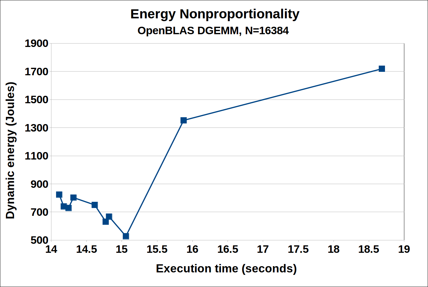
Figure 1 illustrates the energy nonproportionality on S2 found by our method for OpenBLAS DGEMM application solving workload size, N=16384. Data points in the graph represent different configurations of the multithreaded application solving exactly the same problem. Energy proportionality is signified by a monotonically increasing relationship between energy and execution time. This is clearly not the case for the relationship shown in the figure.

Figure 1: Energy nonproportionality on S2 found by our method for OpenBLAS DGEMM application solving workload size, N=16384.

The average and maximum performance improvements using the number of threadgroups and the number of threads per group as decision variables for performance optimization on a single-socket multicore CPU (S1) are (7%, 26.3%), (5%, 6.5%) and (27%, 69%) for the OpenBLAS DGEMM, Intel MKL DGEMM and Intel MKL FFT applications against their best single threadgroup configurations. Along with performance optimization, the energy improvements for OpenBLAS DGEMM and Intel MKL DGEMM are (7.9%, 30%) and (35.7%, 67%) against their best single threadgroup configurations.

At the same time, the optimization for performance alone results in average and maximum increases in dynamic energy consumption of (22.5%, 67%) and (87%, 89%) for the Intel MKL DGEMM and Intel MKL FFT applications in comparison with their energy-optimal configurations. The optimization for dynamic energy alone results in average and maximum performance degradations of (27%, 39%) and (19.7%, 38.2%) in comparison with their performance-optimal configurations. The average and the maximum number of globally Pareto-optimal solutions for Intel MKL DGEMM and Intel MKL FFT are (2.3, 3) and (2.6, 3).

On the 24-core dual-socket CPU (S2), the average and maximum performance improvements of (16%, 20%) and (8%, 21%) for the OpenBLAS DGEMM and Intel MKL DGEMM applications against their best single-threadgroup configurations. Even higher average and maximum performance improvements of (30%, 50%) are achieved for the FFTW application on the 56-core dual-socket CPU (S4). Again, the improvements are measured against the original single-threadgroup basic routine employing optimal number of threads.

At the same time, we find that optimization of the OpenBLAS DGEMM and Intel MKL DGEMM applications on S2 for performance only, results in average and maximum increases in dynamic energy consumption of (15%, 35%) and (7.1%, 49%) in comparison with their energy-optimal configurations, and optimization of the Intel MKL FFT and FFTW applications on S4 for performance alone results in average and maximum increases in dynamic energy consumption of (7%, 25%) and (15%, 57%).

On S2, the optimization of the OpenBLAS DGEMM and Intel MKL DGEMM applications for energy only, results in average and maximum performance degradations of (2.5%, 6%) and (3.7%, 11%). On S4, the average and maximum performance degradations are (20%, 33%) and (31%, 49%) for the Intel MKL FFT and FFTW applications. The performance degradations are over the performance-optimal configuration.

By solving the bi-objective optimization problem on three servers {S1,S2,S4}, the average and the maximum number of globally Pareto-optimal solutions determined by out method are (2.7, 3), (3,11), (2.4, 5) and (1.8, 4) for Intel MKL FFT, FFTW, OpenBLAS DGEMM and Intel MKL DGEMM applications. Finally, we propose a qualitative dynamic energy model based on linear regression and employing performance monitoring counters (PMCs) as parameters, which we use to explain the discovered energy nonproportionality and the Pareto-optimal solutions determined by our method.

The main contributions in this work are the following:

• We show that energy proportionality does not hold true for multicore CPUs thereby affording an opportunity for bi-objective optimization for performance and energy.

• We propose and study the first application-level method for bi-objective optimization of multithreaded data-parallel applications for performance and energy. The method uses two decision variables, the number of identical multithreaded kernels (threadgroups) and the number of threads in each threadgroup. Using four highly optimized data-parallel applications, the proposed method is shown to determine good numbers of globally Pareto-optimal configurations of the applications providing the programmers better trade-offs between performance and energy consumption.

• A qualitative dynamic energy model based on linear regression and employing performance monitoring counters (PMCs) as parameters is proposed to explain the Pareto-optimal solutions determined by our solution method for multicore CPUs. The model shows that the energy nonproportionality on our experimental platforms for the two data-parallel applications is due to disproportionately high energy consumption by the data translation lookaside buffer (dTLB) activity.

The rest of the paper is organized as follows. Section 2 presents the related work. Section 3 contains brief background on multi-objective optimization and the concept of Pareto-optimality. Section 4 describes our solution method. Section 5 describes the first step of our solution method for two data-parallel applications, 2D fast Fourier transform and matrix-matrix multiplication. Section 7 contains the experimental results. Section 7.4 presents our dynamic energy model employing PMCs as parameters to explain the cause behind the energy nonproportionality on our experimental platforms. Section 8 concludes the paper.

2 Related Work

We present an overview of single-objective optimization solution methods for performance or energy followed by bi-objective optimization solution methods for both performance and energy on multicore CPU platforms. Energy models of computing complete the section.

2.1 Performance Optimization

There are three dominant approaches in this category. First category contains research works [22, 23] that have proposed contention-aware thread-level schedulers that try to minimize performance losses due to contention for on-chip shared resources.

The second category includes DRAM controller schedulers that aim to efficiently utilize the shared resource, which is the DRAM memory system, and last level cache partitioning that physically partition the shared resources to minimize contention. DRAM controller schedulers [24, 25] improve the throughput by ordering threads and prioritizing their memory requests through DRAM controllers. Last level cache partitioners [26, 27] explicitly partition the cache when the default cache replacement policies (such as least-recently-used (LRU)) do not result in efficient execution of applications. These partitioners, however, must be used in conjunction with schedulers that mitigate contention for memory controllers and on-chip interconnects.

The final category includes research works that focus on thread-level schedulers that exploit data sharing between the threads to co-schedule them [28, 29]. A key building work in the schedulers are performance models based on PMCs that can predict performance loss due to co-scheduling or migrating threads between cores.

2.2 Energy Optimization

There are three important categories dealing with energy optimization on multicore CPU platforms. The software category contains research works that propose shared resource partitioners. The two hardware categories concern research works that employ Dynamic Voltage and Frequency Scaling (DVFS) and Dynamic Power Management (DPM) and thermal management. Zhuravlev et al. [30] survey the prominent works in all the three categories.

Research works [8, 9] propose dynamic reconfiguration of private caches and partitioning of shared caches (last level cache, for example) to reduce the energy consumption without hurting performance.

DVFS and DPM allow changing the frequencies of the cores and to lower their power states when they are idle. Considering the enormity of literature in this category, we will cover only works that take into account resource contention and thread-to-core mapping while employing DVFS. Kadayif et al. [31] exploit the heterogeneous nature of workloads executed by different processors to set their frequencies so as to reduce energy without impacting performance. Research works [32, 33] employ DVFS to reduce resource contention and energy consumption.

The main goal of thermal management algorithms is to find thread-to-core mappings (or even thread migration) to remove drastic variations in temperatures or thermal hotspots in the chip and at the same time reduce the energy consumption without impacting the performance. They employ as inputs thermal models that are built using temperature measurements provided by on-chip sensors [11, 12]. The algorithms are chiefly employed at the OS level.

Asymmetry-aware schedulers have been proposed for energy optimization on asymmetric multicore systems, which feature a mix of fast and slow cores, high-power and low-power cores but that expose the same instruction-set architecture (ISA). Fedorova et al. [34] propose a system-level scheduler that assigns sequential phases of an application to fast cores and parallel phases to slow cores to maximize the energy efficiency. Herbert et al. [35] employ DVFS to exploit the core-to-core variations from fabrication in power and performance to improve the energy efficiency of the multicore platform.

2.3 Optimization for Performance and Energy

Das et al. [36] propose task mapping to optimize for energy and reliability on multiprocessor systems-on-chip (MPSoCs) with performance as a constraint. Sheikh et al. [37] propose task scheduler employing evolutionary algorithms to optimize applications on multicore CPU platforms for performance, energy, and temperature. Abdi et al. [38] propose multi-criteria optimization where they minimize the execution time under three constraints, the reliability, the power consumption, and the peak temperature. DVFS is a key decision variable in all of these research works.

The following research works focus on application-level solution methods. Subramaniam et al. [39] use multi-variable regression to study the performance-energy trade-offs of the high-performance LINPACK (HPL) benchmark. They study performance-energy trade-offs using the decision variables, number of threads and number of processes. Marszalkowski et al. [40] analyze the impact of memory hierarchies on time-energy trade-off in parallel computations, which are represented as divisible loads. They represent execution time and energy by two linear functions on problem size, one for in-core computations and the other for out-of-core computations.

Research works [3, 5] propose data partitioning algorithms that solve single-objective optimization problems of data-parallel applications for performance or energy on homogeneous clusters of multicore CPUs. They take as an input, discrete performance and dynamic energy functions with no shape assumptions and that accurately and realistically account for resource contention and NUMA inherent in modern multicore CPU platforms. Research work [4] proposes a solution method to solve bi-objective optimization problem of an application for performance and energy on homogeneous clusters of modern multicore CPUs. They demonstrate that the method gives a diverse set of globally Pareto-optimal solutions and that it can be combined with DVFS-based multi-objective optimization methods to give a better set of (globally Pareto-optimal) solutions. The methods target homogeneous HPC platforms. Chakraborti et al. [41] consider the effect of heterogeneous workload distribution on bi-objective optimization of data analytics applications by simulating heterogeneity on homogeneous clusters. The performance is represented by a linear function of problem size and the total energy is predicted using historical data tables. Khaleghzadeh et al. [21] propose a solution method solving the bi-objective optimization problem on heterogeneous processors and comprising of two principal components. The first component is a data partitioning algorithm that takes as an input discrete performance and dynamic energy functions with no shape assumptions. The second component is a novel methodology employed to build the discrete dynamic energy profiles of individual computing devices, which are input to the algorithm.

2.4 Energy Predictive Models of Computation

Energy predictive models predominantly employ performance monitoring counters (PMCs) as parameters. Bellosa et al. [42] propose an energy model based on performance monitoring counters such as integer operations, floating-point operations, memory requests due to cache misses, etc. that they believed to strongly correlate with energy consumption. A linear model that is based on the utilization of CPU, disk, and network is presented in [43]. A more complex power model (Mantis) [44] employs utilization metrics of CPU, disk, and network components and hardware performance counters for memory as predictor variables.

Fan et al. [45] propose a simple linear model that correlates power consumption of a single-core processor with its utilization. Bertran et al. [46] present a power model that provides per-component power breakdown of a multicore CPU. Dargie et al. [47] use the statistics of CPU utilization (instead of PMCs) to model the relationship between the power consumption of multicore processor and workload quantitatively. They demonstrate that the relationship is quadratic for single-core processor and linear for multicore processors. Lastovetsky et al. [3] present an application-level energy model where the dynamic energy consumption of a processor is represented by a discrete function of problem size, which is shown to be highly non-linear for data-parallel applications on modern multicore CPUs.

3 Multi-Objective Optimization: Background

A multi-objective optimization (MOP) problem may be defined as follows [48],[49]:

$$minimize\quad\{\mathcal{F}(x)=(f_{1}(x),...,f_{k}(x))\}$$

$$\text{Subject to}\quad x\in\mathcal{S}$$

where there are $k(\geq 2)$ objective functions $f_{i}:\mathbb{R}^{p}\rightarrow\mathbb{R}$. The objective is to minimize all the objective functions simultaneously.

$\mathcal{F}(x)=(f_{1}(x),...,f_{k}(x))^{T}$ denotes the vector of objective functions. The decision (variable) vectors $x=(x_{1},...,x_{p})$ belong to the (non-empty) feasible region (set) $\mathcal{S}$, which is a subset of the decision variable space $\mathbb{R}^{p}$. We call the image of the feasible region represented by $\mathcal{Z}$ ($=f(\mathcal{S})$), the feasible objective region. It is a subset of the objective space $\mathbb{R}^{k}$. The elements of $\mathcal{Z}$ are called objective (function) vectors or criterion vectors and denoted by $\mathcal{F}(x)$ or $z=(z_{1},...,z_{k})^{T}$, where $z_{i}=f_{i}(x),\forall i\in[1,k]$ are objective (function) values or criterion values.

If there is no conflict between the objective functions, then a solution $x^{*}$ can be found where every objective function attains its optimum [49].

$$\forall x\in\mathcal{S},f_{i}(x^{*})\leq f_{i}(x),\quad i=1,...,k$$

However, in real-life multi-objective optimization problems, the objective functions are at least partly conflicting. Because of this conflicting nature of objective functions, it is not possible to find a single solution that would be optimal for all the objectives simultaneously. In multi-objective optimization, there is no natural ordering in the objective space because it is only partially ordered. Therefore we must treat the concept of optimality differently from single-objective optimization problem. The generally used concept is Pareto-optimality.

Definition 1.

A decision vector $x^{*}\in\mathcal{S}$ is Pareto-optimal if there does not exist another decision vector $x\in\mathcal{S}$ such that $f_{i}(x)\leq f_{i}(x^{*}),\forall i=1,...,k$ and $f_{j}(x)<f_{j}(x^{*})$ for at least one index $j$ [48].

An objective vector $z^{*}\in\mathcal{Z}$ is Pareto-optimal if there does not exist another objective vector $z\in\mathcal{Z}$ such that $z_{i}\leq z_{i}^{*},\forall i=1,...,k$ and $z_{j}<z_{j}^{*}$ for at least one index $j$.

Definition 2.

A decision vector $x^{*}\in\mathcal{S}$ is weakly Pareto-optimal if there does not exist another decision vector $x\in\mathcal{S}$ such that $f_{i}(x)<f_{i}(x^{*}),\forall i=1,...,k$ [48].

An objective vector $z^{*}\in\mathcal{Z}$ is Pareto-optimal if there does not exist any other vector for which all the component objective vector values are better.

Mathematically speaking, every Pareto-optimal point is an equally acceptable solution of the multi-objective optimization problem. Therefore, user preference relations (or preferences of decision maker) are provided as input to the solution process to select one or more points from the set of Pareto-optimal solutions [48].

Figure 2: An example showing the set $\mathcal{S}$ of decision variable vectors, the set $\mathcal{Z}$ of objective vectors, and Pareto-optimal objective vectors shown by bold line. $\mathcal{S}\subset\mathbb{R}^{3},\mathcal{Z}\subset\mathbb{R}^{2}$.

(a)

(b)

(c)

Figure 3: (a). PMMTG-V: Matrices B and C are vertically partitioned among the threadgroups. (b). PMMTG-H: Matrices A and C are horizontally partitioned among the threadgroups. (c). PMMTG-S: The $p$ threadgroups are arranged in a square grid of size $\sqrt{p}\times\sqrt{p}$. All the matrices are partitioned into squares among the threadgroups.

Figure 4: 2D-DFT of signal matrix M of size $N\times N$ using $p$ threadgroups. a). PFFTTG-V using vertical decomposition of the signal matrix. b). PFFTTG-H using horizontal decomposition of the signal matrix.

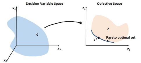
In Figure 2, a feasible region $\mathcal{S}\subset\mathbb{R}^{3}$ and its image, a feasible objective region $\mathcal{Z}\subset\mathbb{R}^{2}$, are shown. The thick blue line in the figure showing the objective space contains all the Pareto-optimal objective vectors. The vector $z^{*}$ is one of them.

In this work, we consider bi-objective optimization where performance and dynamic energy are the objectives.

4 Solution Method Solving Bi-objective Optimization Problem on a Single Multicore CPU

In this section, we describe our solution method, BOPPETG, for solving the bi-objective optimization problem of a multithreaded data-parallel application on multicore CPUs for performance and energy (BOPPE). The method uses two decision variables, the number of identical multithreaded kernels (threadgroups) and the number of threads in each threadgroup. A given workload is always partitioned equally between the threadgroups.

The bi-objective optimization problem (BOPPE) can be formulated as follows: Given a multithreaded data-parallel application of workload size $n$ and a multicore CPU of $l$ cores, the problem is to find a globally Pareto-optimal front of solutions optimizing execution time and dynamic energy consumption during the parallel execution of the workload. Each solution is an application configuration given by (threadgroups, threads per group).

The inputs to the solution method are the workload size of the multi-threaded data-parallel application, $n$; the number of cores in the multicore CPU, $l$; the multithreaded base kernel, $mtkernel$; the base power of the multicore CPU platform, $P_{b}$. The outputs are the globally Pareto-optimal front of objective solutions, $\mathcal{P}_{opt}$, and the optimal application configurations corresponding to these solutions, $\mathcal{C}_{opt}$. Each Pareto-optimal solution of objectives $o$ is represented by the pair, $(s_{o},e_{o})$, where $s_{o}$ is the execution time and $e_{o}$ is the dynamic energy. Associated with this solution is an array of application configurations, $\mathcal{A}(g_{o},t_{o})$, containing decision variable pairs, $(g_{o},t_{o})$, where $g_{o}$ represents the number of threadgroups each containing $t_{o}$ threads.

The main steps of BOPPETG are as follows:

Step 1. Parallel implementation allowing ($g$,$t$) configuration: Design and implement a data-parallel version of the base kernel $mtkernel$ and that can be executed using $g$ identical multithreaded kernels in parallel. Each kernel is executed by a threadgroup containing $t$ threads. The workload $n$ is divided equally between the $g$ threadgroups during the execution of the data-parallel version. The data-parallel version should essentially allow its runtime configuration using number of threadgroups and number of threads per group with the workload equally partitioned between the threadgroups.

Step 2. Initialize $g$ and $t$: All the runtime configurations, ($g$,$t$), where the product, $g\times t$, is less than or equal to the total number of cores ($l$) in the multicore platform are considered. $g\leftarrow 1$, $t\leftarrow 1$. Go to Step 3.

Step 3. Determine time and dynamic energy of the ($g$,$t$) configuration of the application: The data-parallel version composed in Step 1 is run using the ($g$,$t$) configuration. Its execution time and dynamic energy consumption are determined as follows: $s_{o}=t_{f}-t_{i}$, $e_{o}=e_{f}-P_{b}\times s_{o}$, where $t_{i}$ and $t_{f}$ are the starting and ending execution times and $e_{f}$ is the total energy consumption during the execution of the application. Go to Step 4.

Step 4. Update Pareto-optimal front for ($g$,$t$): The solution $(s_{o},e_{o})$ if Pareto-optimal is added to the globally Pareto-optimal set of objective solutions, $\{\mathcal{P}_{opt}\}$, and existing member solutions of the set that are inferior to it are removed. The optimal application configurations corresponding to the solution $(s_{o},e_{o})$ are stored in $\mathcal{C}_{opt}$. Go to Step 5.

Step 5. Test and Increment ($g$,$t$): If $t<l$, $t\leftarrow t+1$, go to Step 3. Set $g\leftarrow g+1$, $t\leftarrow 1$. If $g\times t\leq l$, go to Step 3. Else return the globally Pareto-optimal front and optimal application configurations given by $\{\mathcal{P}_{opt},\mathcal{C}_{opt}\}$ and quit.

In the following section, we illustrate the first step of BOPPETG for two applications, matrix-matrix multiplication and 2D fast Fourier transform. We show in particular how BOPPETG can reuse highly optimized scientific kernels with careful design and development of parallel versions of the application.

5 Parallel Matrix-Matrix Multiplication

We illustrate the first step of our solution method (BOPPETG) for implementing the data-parallel version of dense matrix-matrix multiplication (PMMTG).

⬇

1void *dgemm(void *input)

2{

3 int i = *(int*)input;

4 openblas_set_num_threads(t);

5 goto_set_num_threads(t);

6 omp_set_num_threads(t);

7 if (i == 1)

8 {

9 cblas_dgemm(CblasRowMajor, CblasNoTrans,

10 CblasNoTrans, N/p, N, N, alpha, A1, N,

11 B, N, beta, C1, N);

12 }

13 …

14 if (i == p)

15 {

16 cblas_dgemm(CblasRowMajor, CblasNoTrans,

17 CblasNoTrans, N/p, N, N, alpha, Ap, N,

18 B, N, beta, Cp, N);

19 }

20}

21

22int main() {

23 int row;

24#pragma omp parallel for num_threads(p*t)

25 for (row = 0; row < N/p; row++) {

26 memcpy(&A1[row*N], &A[row*N], N*sizeof(double));

27 …

28 memcpy(&Ap[row*N], &A[(p-1)*N*(N/p)+row*N],

29 N*sizeof(double));

30 memcpy(&C1[row*N], &C[row*N], N*sizeof(double));

31 …

32 memcpy(&Cp[row*N], &C[(p-1)*N*(N/p)+row*N],

33 N*sizeof(double));

34 }

35

36 pthread_t t1, …, tp;

37 int i1 = 1, …, ip = p;

38 pthread_create(&t1, NULL, dgemm, &i1);

39 …

40 pthread_create(&tp, NULL, dgemm, &ip);

41 pthread_join(tp, NULL);

42 …

43 pthread_join(t1, NULL);

44

45#pragma omp parallel for num_threads(p*t)

46 for (row = 0; row < N/p; row++)

47 {

48 memcpy(&A[row*N], &A1[row*N], N*sizeof(double));

49 …

50 memcpy(&A[(p-1)*N*(N/p)+row*N], &Ap[row*N],

51 N*sizeof(double));

52 memcpy(&C[row*N], &C1[row*N], N*sizeof(double));

53 …

54 memcpy(&C[(p-1)*N*(N/p)+row*N], &Cp[row*N],

55 N*sizeof(double));

56 }

57}

Figure 5: OpenBLAS implementation of parallel matrix-matrix multiplication using horizontal decomposition (PMMTG-H) and employing $p$ threadgroups of $t$ threads each.

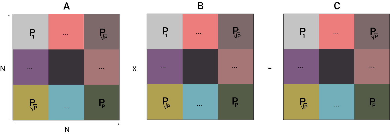
The PMMTG application computes the matrix product ($C=\alpha\times A\times B+\beta\times C$) of two dense square matrices A and B of size $N\times N$. The application is executed using $p$ threadgroups, $\{P_{1},...,P_{p}\}$. To simplify the exposition of the algorithms, we assume N to be divisible by p.

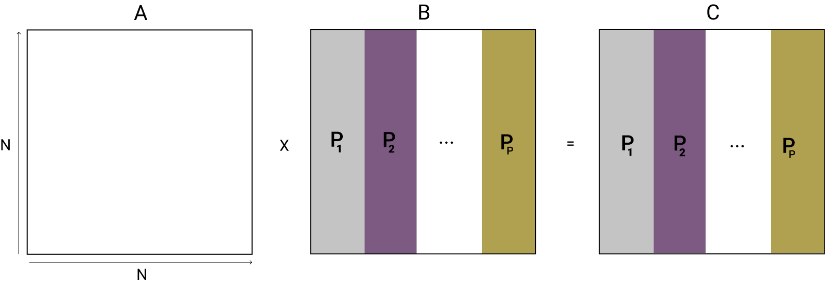
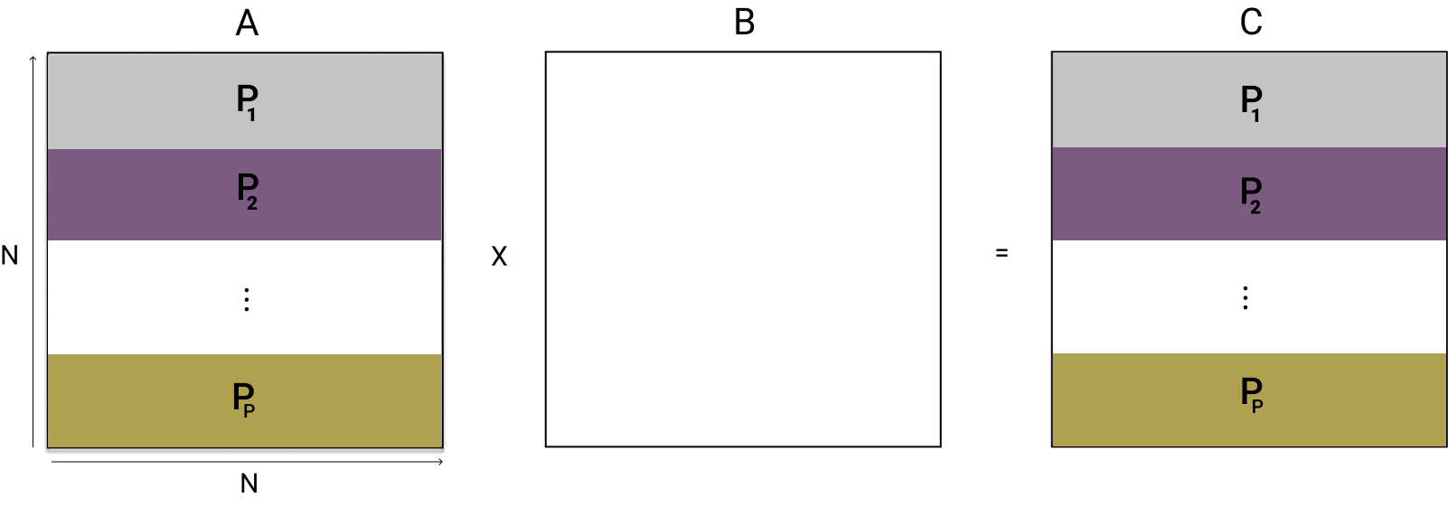
There are three parallel algorithmic variants of PMMTG. In PMMTG-V, the matrices B and C are partitioned vertically such that each threadgroup is assigned $\frac{N}{p}$ of the columns of B and C as shown in the Figure 3a. Each threadgroup $P_{i}$ computes its vertical partition $C_{P_{i}}$ using the matrix product, $C_{P_{i}}=\alpha\times A\times B_{P_{i}}+\beta\times C_{P_{i}}$. In PMMTG-H, the matrices A and C are partitioned horizontally such that each threadgroup is assigned $\frac{N}{p}$ of the rows of B and C as shown in the Figure 3b. Each threadgroup $P_{i}$ computes its horizontal partition $C_{P_{i}}$ using the matrix product, $C_{P_{i}}=\alpha\times A_{P_{i}}\times B+\beta\times C_{P_{i}}$. In PMMTG-S, the $p$ threadgroups $\{P_{1},...,P_{p}\}$ are arranged in a square grid $Q_{st},s\in[1,\sqrt{p}],t\in[1,\sqrt{p}]$. The matrices A, B, and C are partitioned into equal squares among the threadgroups as shown in the Figure 3c. In each matrix, each threadgroup $P_{i}(=Q_{st})$ is assigned a sub-matrix of size $\frac{N}{\sqrt{p}}\times\frac{N}{\sqrt{p}}$ and computes its square partition $C_{Q_{st}}$ using the matrix product, $C_{Q_{st}}=\alpha\times\sum_{k=1}^{\sqrt{p}}(A_{sk}\times B_{kt})+\beta\times C_{Q_{st}}$. $A_{sk}$ is the square block in matrix $A$ located at $(s,k)$. $B_{kt}$ is the square block in matrix $B$ located at $(k,t)$.

5.1 Implementation of PMMTG-H Based on OpenBLAS DGEMM

We describe an OpenBLAS implementation of PMMTG-H (Figure 5) here. The implementations of the other PMMTG algorithms employing Intel MKL and OpenBLAS are described in the supplemental.

The inputs to an implementation are: a). Matrices A, B, and C of sizes $N\times N$; b). Constants $\alpha$ and $\beta$; c) The number of threadgroups, $\{P_{1},\cdots,P_{p}\}$; d). The number of threads in each threadgroup represented by $t$. The output matrix, C, contains the matrix product.

The vertical partitions of A and C, {$A_{P_{i}},C_{P_{i}}$}, $i\in[1,p]$, assigned to the threadgroups, $\{P_{1},...,P_{p}\}$, are initialized in Lines 24-34. Then $p$ pthreads representing the $p$ threadgroups are created, each a multithreaded OpenBLAS DGEMM kernel executing $t$ OpenMP threads (Lines 36-43).The $p$ threadgroups compute the matrix-matrix product (Lines 1-20). The result is gathered in the matrix C (Lines 45-56).

The implementations using Intel MKL differ from those using OpenBLAS. In Intel MKL, the matrix-matrix computation by a threadgroup is performed using an OpenMP parallel region with $t$ threads whereas the same is done in OpenBLAS using a pthread.

6 Parallel 2D Fast Fourier Transform

We present here the first step of our solution method (BOPPETG) to compose the data-parallel version of 2D Fast Fourier Transform (PFFTTG). The sequential 2D FFT algorithm is described first before the two parallel algorithmic variants of 2D Fast Fourier Transform.

The definition of 2D-DFT of a two-dimensional point discrete signal M of size $N\times N$ is below:

$$M[k][l] =\sum_{i=0}^{N-1}\sum_{j=0}^{N-1}M[i][j]\times\omega_{N}^{ki}\times\omega_{N}^{lj}$$

$$\omega_{N} =e^{-\frac{2\pi}{N}},0\leq k,l\leq N-1$$

M is the signal matrix where each element $M[i][j]$ is a complex number. The total number of complex multiplications required to compute the 2D-DFT is $\Theta(N^{4})$.

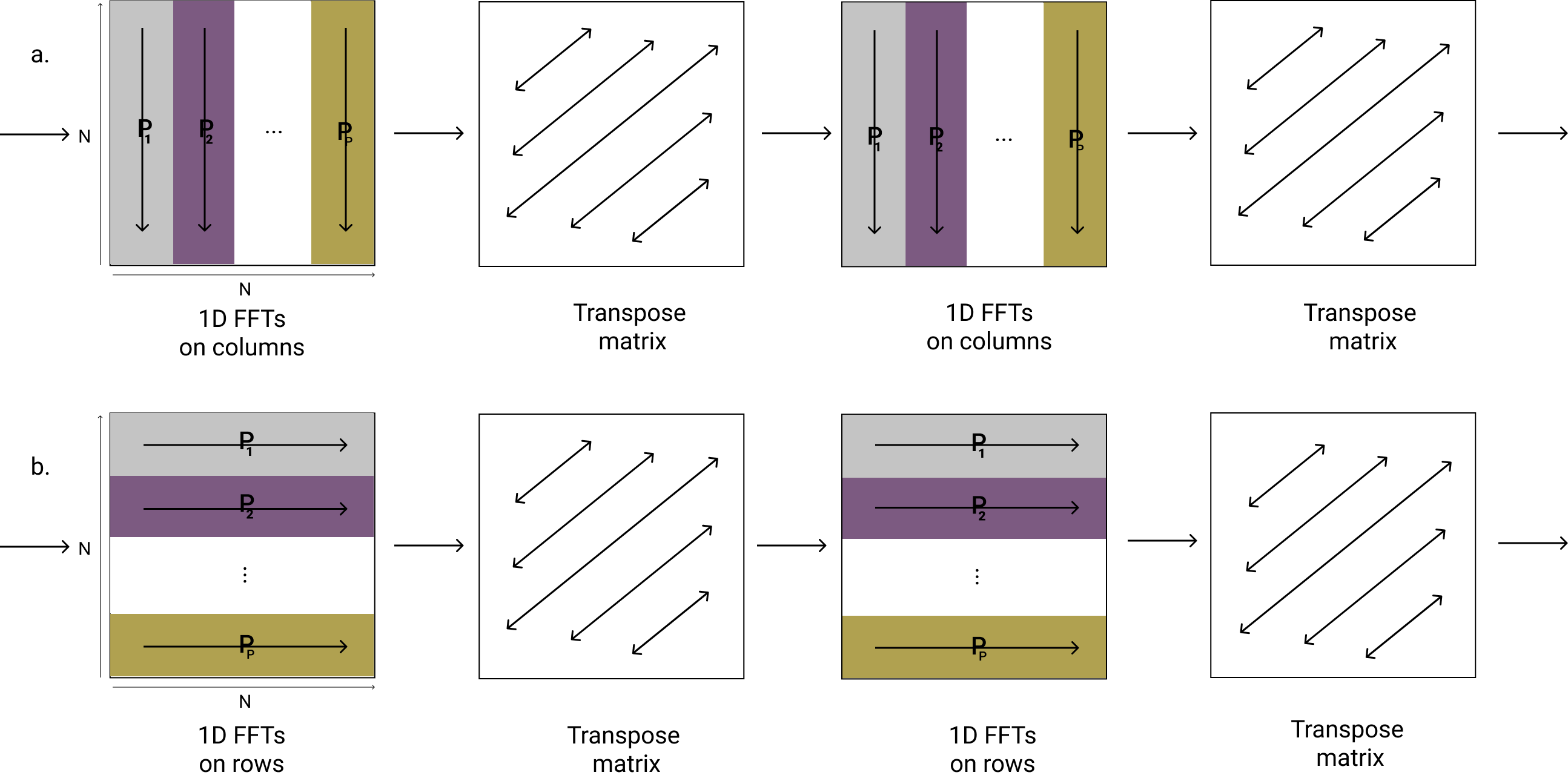
The sequential row-column decomposition method reduces this complexity by computing the 2D-DFT using a series of 1D-DFTs, which are implemented using a fast 1D-FFT algorithm. The method consists of two phases called the row-transform phase and column-transform phase. Figure 4 depicts the method, which is mathematically summarized below:

$$M[k][l] =\sum_{i=0}^{N-1}\sum_{j=0}^{N-1}M[i][j]\times\omega_{N}^{ki}\times\omega_{N}^{lj}$$

$$=\sum_{i=0}^{N-1}\omega_{N}^{ki}\times(\sum_{j=0}^{N-1}M[i][j]\times\omega_{N}^{lj})$$

$$=\sum_{i=0}^{N-1}\omega_{N}^{ki}\times(\tilde{M}[i][l])$$

$$=\sum_{i=0}^{N-1}(\tilde{M}[i][l])\times\omega_{N}^{ki}$$

$$\omega_{N} =e^{-\frac{2\pi}{N}},0\leq k,l\leq N-1$$

It computes a series of ordered 1D-FFTs of size N on the N rows. That is, each row i (of length N) is transformed via a fast 1D-FFT to $\tilde{M}[i][l],\forall l\in[0,N-1]$. The total cost of this row-transform phase is $\Theta(N^{2}\log_{2}N)$. Then, it computes a series of ordered 1D-FFTs on the N columns of $\tilde{M}$. The column $l$ of $\tilde{M}$ is transformed to $M[k][l],\forall k\in[0,N-1]$. The total cost of this column-transform phase is $\Theta(N^{2}\log_{2}N)$. Thus, by using the row-column decomposition method, the complexity of 2D-FFT is reduced from $\Theta(N^{4})$ to $\Theta(N^{2}\log_{2}N)$. All the FFTs that we discuss in this work are considered in-place.

The PFFTTG application employing our solution method computes the 2D-DFT of the signal matrix of size $N\times N$ using $p$ threadgroups, $\{P_{1},...,P_{p}\}$. It is based on the sequential 2D-FFT row-column decomposition method. There are two parallel algorithmic variants of PFFTTG, PFFTTG-H and PFFTTG-V. To simplify the exposition of the algorithms, we assume N to be divisible by p.

6.1 PFFTTG-H: Using Horizontal Decomposition of Signal Matrix $M$

The parallel 2D-FFT algorithm, PFFTTG-H, consists of four steps:

Step 1. 1D-FFTs on rows: Threadgroup $P_{i}$ executes sequential 1D-FFTs on rows $(i-1)\times\frac{N}{p}+1,...,i\times\frac{N}{p}$.

Step 2. Matrix Transposition: Transpose the matrix M.

Step 3. 1D-FFTs on rows: Threadgroup $P_{i}$ executes sequential 1D-FFTs on rows $(i-1)\times\frac{N}{p}+1,...,i\times\frac{N}{p}$.

Step 4. Matrix Transposition: Transpose the matrix M.

The computational complexity of Steps 1 and 3 is $\Theta(\frac{N^{2}}{p}\log_{2}N)$. The computational complexity of Steps 2 and 4 is $\Theta(\frac{N^{2}}{p})$. Therefore, the total computational complexity of PFFTTG-H is $\Theta(\frac{N^{2}}{p}\log_{2}N)$.

The algorithm is illustrated in the Figure 4.

6.2 PFFTTG-V: Using Vertical Decomposition of Signal Matrix $M$

The parallel 2D-FFT algorithm, PFFTTG-V, consists of four steps:

Step 1. 1D-FFTs on columns: Threadgroup $P_{i}$ executes sequential 1D-FFTs on columns $(i-1)\times\frac{N}{p}+1,...,i\times\frac{N}{p}$.

Step 2. Matrix Transposition: Transpose the matrix M.

Step 3. 1D-FFTs on columns: Threadgroup $P_{i}$ executes sequential 1D-FFTs on columns $(i-1)\times\frac{N}{p}+1,...,i\times\frac{N}{p}$.

Step 4. Matrix Transposition: Transpose the matrix M.

The computational complexity of Steps 1 and 3 is $\Theta(\frac{N^{2}}{p}\log_{2}N)$. The computational complexity of Steps 2 and 4 is $\Theta(\frac{N^{2}}{p})$. Therefore, the total computational complexity of PFFTTG-V is $\Theta(\frac{N^{2}}{p}\log_{2}N)$.

The algorithm is illustrated in the Figure 4.

⬇

1fftw_plan fftw1d_init_plan(const int sign, const int m,

2 const int n, fftw_complex* X, fftw_complex* Y)

3{

4 int rank = 1, howmany = m;

5 int s[] = {n}, idist = n;

6 int odist = n, istride = 1;

7 int ostride = 1, *inembed = s, *onembed = s;

8 return fftw_plan_many_dft(rank, s, howmany,

9 X, inembed, istride, idist, Y, onembed,

10 ostride, odist, sign, FFTW_ESTIMATE);

11}

12int fftw2d(const int sign, const int p, const int N,

13 const unsigned int t, const unsigned int blockSize,

14 fftw_complex* X

15)

16{

17 fftw_init_threads();

18 fftw_plan_with_nthreads(t);

19 fftw_plan plan1, plan2, …, planp;

20 plan1 = fftw1d_init_plan(sign, N/p, N, X, X);

21 plan2 = fftw1d_init_plan(sign, N/p, N,

22 &X[(N/p)*N], &X[(N/p)*N]);

23 …

24 planp = fftw1d_init_plan(sign, N-(p-1)*(N/p), N,

25 &X[(p-1)*(N/p)*N], &X[(p-1)*(N/p)*N]);

26#pragma omp parallel sections num_threads(p)

27{

28 #pragma omp section

29 {

30 fftw_execute(plan1);

31 fftw_destroy_plan(plan1);

32 }

33…

34 #pragma omp section

35 {

36 fftw_execute(plan12);

37 fftw_destroy_plan(plan12);

38 }

39}

40 hcl_transpose_block(X, 0, N, N, t, blockSize);

41 plan1 = fftw1d_init_plan(sign, N/p, N, X, X);

42 plan2 = fftw1d_init_plan(sign, N/p, N,

43 &X[(N/p)*N], &X[(N/p)*N]);

44 …

45 planp = fftw1d_init_plan(sign, N-(p-1)*(N/p), N,

46 &X[(p-1)*(N/p)*N], &X[(p-1)*(N/p)*N]);

47#pragma omp parallel sections num_threads(p)

48{

49 #pragma omp section

50 {

51 fftw_execute(plan1);

52 fftw_destroy_plan(plan1);

53 }

54…

55 #pragma omp section

56 {

57 fftw_execute(plan12);

58 fftw_destroy_plan(plan12);

59 }

60}

61 hcl_transpose_block(X, 0, N, N, nt, blockSize);

62 fftw_cleanup_threads();

63}

Figure 6: FFTW implementation using horizontal decomposition of signal matrix and executed by $p$ threadgroups of $t$ threads each.

6.3 Implementation of PFFTTG-H Based on FFTW

Figure 6 illustrates the FFTW implementation of PFFTTG-H. The shared memory implementations of other PFFTTG algorithms based on Intel MKL and FFTW are described in the supplemental.

The inputs to an implementation are: a). Signal matrix M of size $N\times N$; b). The number of threadgroups, $p$, $\{P_{1},\cdots,P_{p}\}$; c). The number of threads in each threadgroup represented by $t$. The output is the transformed signal matrix M (considering that we are performing in-place FFT).

Lines 17-18 show the initialization of FFTW multithreaded runtime. Lines 19-25 show the creation of $p$ FFT plans, each plan executed by a threadgroup of $t$ threads. Lines 1-11 illustrate the creation of a plan using fftw_dft_plan_many routine. Lines 26-39 show the execution and destruction of the plans (1D-FFTs on rows) by the threadgroups. This is followed by transpose of the signal matrix (Line 40). Lines 41-46 contain the creation of $p$ FFT plans (1D-FFTs on rows) followed by their execution by the threadgroups. Finally, the signal matrix is transposed again (Line 61). The FFTW runtime is then destroyed (Line 62).

The implementations based on Intel MKL differ from those employing FFTW. In FFTW, only plan execution (fftw_plan_many_dft) and plan destruction (fftw_destroy_plan) are thread-safe and can be called in an OpenMP parallel region.

7 Experimental Results and Discussion

In this section, we present our experimental results for matrix-matrix multiplication (PMMTG) and 2D fast Fourier transform (PFFTTG) employing our solution method.

To make sure the experimental results are reliable, we follow a statistical methodology described in the supplemental. Briefly, for every data point in the functions, the automation software executes the application repeatedly until the sample mean lies in the 95% confidence interval and a precision of 0.025 (2.5%) has been achieved. For this purpose, Student’s t-test is used assuming that the individual observations are independent and their population follows the normal distribution. The validity of these assumptions is verified by plotting the distributions of observations and using Pearson’s Test. The speed/time/energy values shown in the graphical plots are the sample means.

Four multicore CPUs shown in the Table IV and described earlier are used in the experiments. Three platforms {S1, S2, S4} have a power meter installed between their input power sockets and the wall A/C outlets. S1 and S2 are connected with a Watts Up Pro power meter; S4 is connected with a Yokogawa WT310 power meter. S3 is not equipped with a power meter and therefore is not employed in the experiments for single-objective optimization for energy and bi-objective optimization for performance and energy.

The power meter provides the total power consumption of the server. It has a data cable connected to one USB port of the server. A script written in Perl collects the data from the power meter using the serial USB interface. The execution of the script is non-intrusive and consumes insignificant power. WattsUp Pro power meters are periodically calibrated using the ANSI C12.20 revenue-grade power meter, Yokogawa WT310. The maximum sampling speed of WattsUp Pro power meters is one sample every second. The accuracy specified in the data-sheets is $\pm{3\%}$. The minimum measurable power is 0.5 watts. The accuracy at 0.5 watts is $\pm{0.3}$ watts. The accuracy of Yokogawa WT310 is 0.1% and the sampling rate is 100k samples per second.

HCLWattsUp API [50] is used to gather the readings from the power meter to determine the dynamic energy consumption during the execution of PMMTG and PFFTTG applications. HCLWattsUp has no extra overhead and therefore does not influence the energy consumption of the application execution.

Fans are significant contributors to energy consumption. On our platform, fans are controlled in two zones: a) zone 0: CPU or System fans, b) zone 1: Peripheral zone fans. There are 4 levels to control the speed of fans:

• Standard: BMC control of both fan zones, with CPU zone based on CPU temp (target speed 50%) and Peripheral zone based on PCH temp (target speed 50%)

• Optimal: BMC control of the CPU zone (target speed 30%), with Peripheral zone fixed at low speed (fixed  30%)

• Heavy IO: BMC control of CPU zone (target speed 50%), Peripheral zone fixed at 75%

• Full: all fans running at 100%

To rule out the contribution of fans in dynamic energy consumption, we set the fans at full speed before executing the applications. When set at full speed, the fans run constantly at ${\sim}13400$ rpm until they are set to a different speed level. In this way, energy consumption due to fans is included only in the static power consumption of the platform. The temperature of our platform and speeds of the fans (with Full setting) is monitored with the help of Intelligent Platform Management Interface (IPMI) sensors, both with and without the application run. An insignificant difference in the speeds of fans is found in both the scenarios.

7.1 Parallel Matrix-Matrix Multiplication Using OpenBLAS DGEMM and Intel MKL DGEMM

7.1.1 Performance Optimization on a Single Socket Multicore CPU

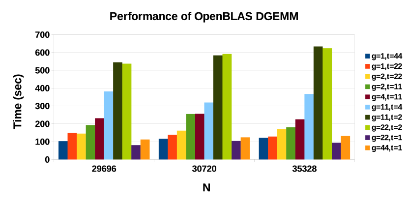
Fiqure 7 shows the execution times of PMMTG using OpenBLAS DGEMM for different threadgroup combinations on a single-socket CPU (S1). The base version corresponds to the application configuration employing one threadgroup with optimal number of threads, which is 44 threads. The best combination is ($g$,$t$)=(22,1) for all the three workload sizes. It outperforms the base combination by 20% for N=29696 and N=35328, and about 11% for N=30720. Furthermore, the average performance improvement over the base combination for 41 tested workload sizes in the range, $5120\leq N\leq 36000$, is 7%. The starting problem size of 5120 is chosen to ensure that the workload size exceeds the last level cache.

Figure 7: Performance of PMMTG application employing OpenBLAS DGEMM for different ($g$,$t$) configurations on S1.

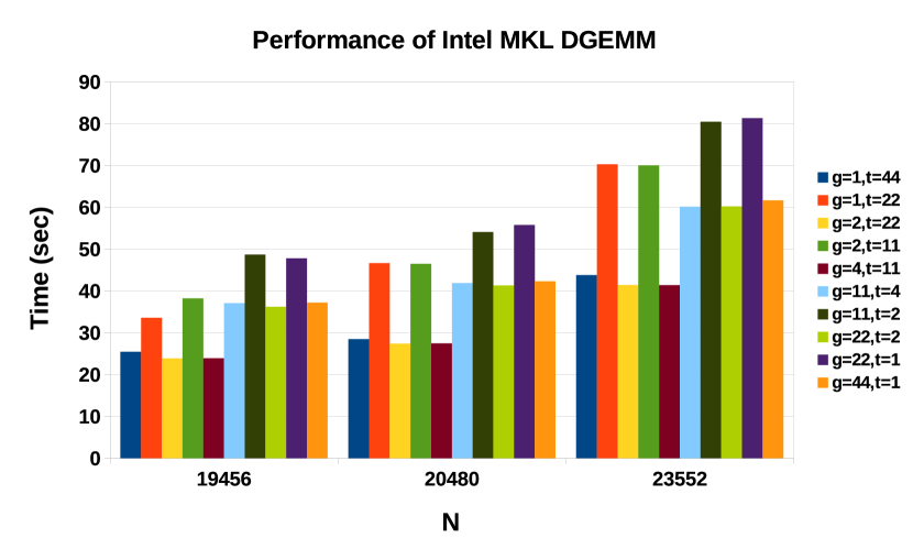
Fiqure 8 shows the execution times of PMMTG using Intel MKL DGEMM. The best combinations ($g$,$t$) are {(4,11),(2,22)} for all the three workload sizes. They outperform the base combination by 6%. The average performance improvement over the base combination for 21 tested workload sizes in the range, $5120\leq N\leq 36000$, is 5%.

Figure 8: Performance of PMMTG application employing Intel MKL DGEMM for different ($g$,$t$) configurations on S1.

7.1.2 Performance Optimization on a Dual-socket Multicore CPU

Figure 9 shows the comparision between base and best combinations for OpenBLAS DGEMM and Intel MKL DGEMM on S3. The base version corresponds to application configuration employing one threadgroup with optimal number of threads.

Figure 9: Comparision between the base and best versions for Intel MKL DGEMM and OpenBLAS DGEMM on S3.

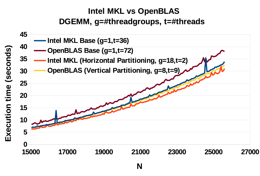
Unlike the base version, the best combinations for OpenBLAS DGEMM and Intel MKL DGEMM do not have any performance variations (drops). The best combination for Intel MKL DGEMM is 18 threadgroups with 2 threads each. It outperforms the base version by 8% on the average and the next best combination, 12 threadgroups with 2 threads each, by 2.5%. Our solution method removed noticeable drops in performance for workload sizes 16384, 20480, and 24576, with performance improvements of 36.5%, 14.5% and 21.5%.

7.1.3 Energy Optimization on a Single Socket Multicore CPU

Fiqure 10 shows the dynamic energy consumptions for PMMTG using OpenBLAS DGEMM of different threadgroup combinations on a single-socket CPU (S1). The base version corresponds to application configuration employing one threadgroup with optimal number of threads, which is 44 threads. The best combination for sizes N=29696 and N=30720 is ($g$,$t$)=(22,1). It outperforms the base combination by 20%. The best combination for $N=35328$ is ($g$,$t$)=(1,22), which outperforms the base combination by 23%. Furthermore, the average improvement (or energy savings) over the base combination for 41 tested workload sizes in the range, $5120\leq N\leq 35000$, is 8%.

Figure 10: Dynamic energy consumption for PMMTG employing OpenBLAS DGEMM for different ($g$,$t$) configurations on S1.

Fiqure 11 shows the dynamic energy consumptions for PMMTG using Intel MKL DGEMM. There are three best combinations for each problem size, ($g$,$t$)={(11,4),(22,2),(44,1)}. They outperform the base combination by 35%. Furthermore, the average improvement over the base combination for 21 tested workload sizes in the range, $5120\leq N\leq 35000$, is 35.7%.

Figure 11: Dynamic energy consumption for PMMTG employing Intel MKL DGEMM for different ($g$,$t$) configurations on S1.

7.1.4 Energy Optimization on a Dual-socket Multicore CPU

Figure 12: Dynamic energy consumption of PMMTG employing OpenBLAS DGEMM for different ($g$,$t$) configurations on S2.

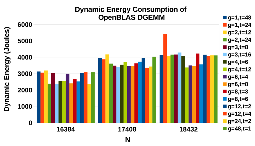
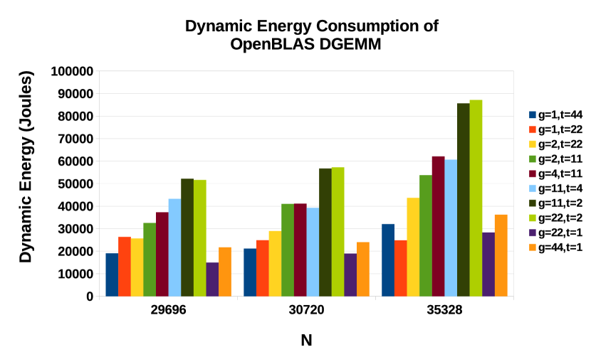
Figure 12 show the results for PMMTG based on OpenBLAS DGEMM on S2 with three different workload sizes. There are four best combinations minimizing the dynamic energy consumption for workload size 16384, ($g$,$t$)={(2,24),(3,16),(6,8),(24,2)}. The energy savings for these combinations compared with the best base combination, ($g$,$t$)=(1,24), is around 21%. For the workload sizes 17408 and 18432, the best combinations are (12,4) and (4,12). The energy savings in comparison with the best base combination, ($g$,$t$)=(1,24), for 17408 and ($g$,$t$)=(1,44) for 18432, are 15% and 18%. Furthermore, the average improvement over the best base combination for 19 tested workload sizes in the range, $5120\leq N\leq 35000$, is 10%.

Figure 13: Dynamic energy consumption of PMMTG employing Intel MKL DGEMM for different ($g$,$t$) configurations on S2.

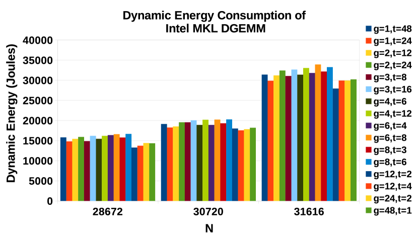
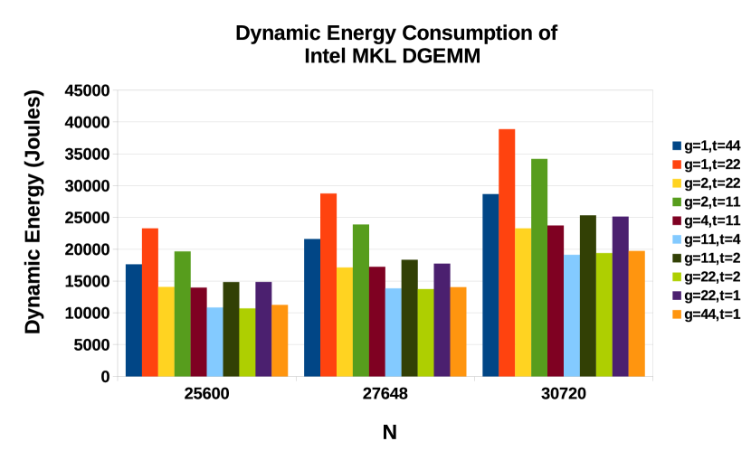
Figure 13 show the results for PMMTG based on Intel MKL DGEMM on S2. The best combination minimizing the dynamic energy consumption for workload size 28672 involves 12 threadgroups with 2 threads each. The energy savings for this combination compared with the best base combination, (1,24), is 10.5%. For the workload sizes 30720 and 31616, the best combinations are (12,4) and (12,2). The energy savings in comparison with the best base combination are 4% and 7%. Furthermore, the average improvement over the best base combination for 19 tested workload sizes in the range, $5120\leq N\leq 35000$, is 13%.

7.2 Parallel 2D Fast Fourier Transform Using FFTW and Intel MKL FFT

In this section, we use 2D fast Fourier transform routines from two packages, FFTW-3.3.7 and Intel MKL. The packages are installed with multithreading, SSE/SSE2, AVX2, and FMA (fused multiply-add) optimizations enabled. For Intel MKL FFT, no special environment variables are used. Three planner flags, {FFTW_ESTIMATE, FFTW_MEASURE, FFTW_PATIENT} were tested. The execution times for the flags {FFTW_MEASURE, FFTW_PATIENT} are high compared to those for FFTW_ESTIMATE. The long execution times are due to the lengthy times to create the plans because FFTW_MEASURE tries to find an optimized plan by computing many FFTs whereas FFTW_PATIENT considers a wider range of algorithms to find a more optimal plan.

7.2.1 Performance Optimization on a Single Socket Multicore CPU

Figure 14 shows the results for PFFTTG employing FFTW on a single-socket CPU (S1). The best combination, ($g,t$)=(4,11), is the same for workload sizes, N=31936 and N=32704. The improvements over the base combination, ($g,t$)=(1,44), are 55% and 57%. For matrix dimension, N=35648, the base combination is the best and outperforms the next best combination, ($g,t$)=(2,22), by 5%.

Figure 14: Performance of PFFTTG employing FFTW for different ($g$,$t$) configurations on S1.

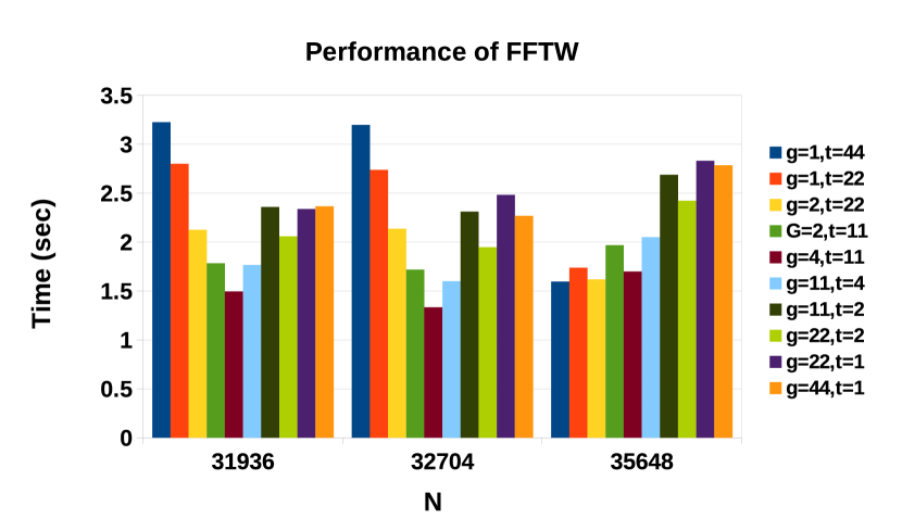
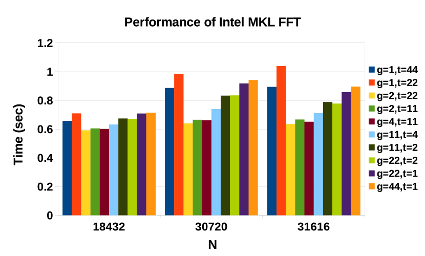
Figure 15 shows the results for PFFTTG employing Intel MKL FFT. There are three best combinations, ($g,t$)=(2,22),(2,11),(4,11), for all the three workload sizes, where performances differ from each other by less than 5%. Their improvement over the base combination, ($g,t$)=(1,44), for N=18432 is 8%. For workload sizes, N=30720 and N=31616, the performance improvements are 25% and 26%. Furthermore, the average performance improvement over the best base combination for 23 tested workload sizes in the range, $5120\leq N\leq 37000$, is 27%.

Figure 15: Performance of PFFTTG employing Intel MKL FFT for different ($g$,$t$) configurations on S1.

7.2.2 Performance Optimization on Dual-socket Multicore CPUs

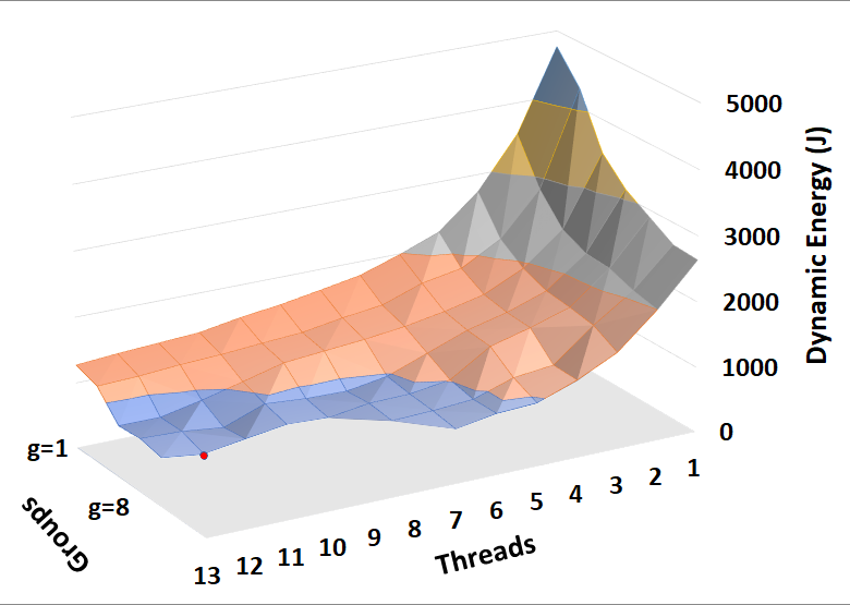
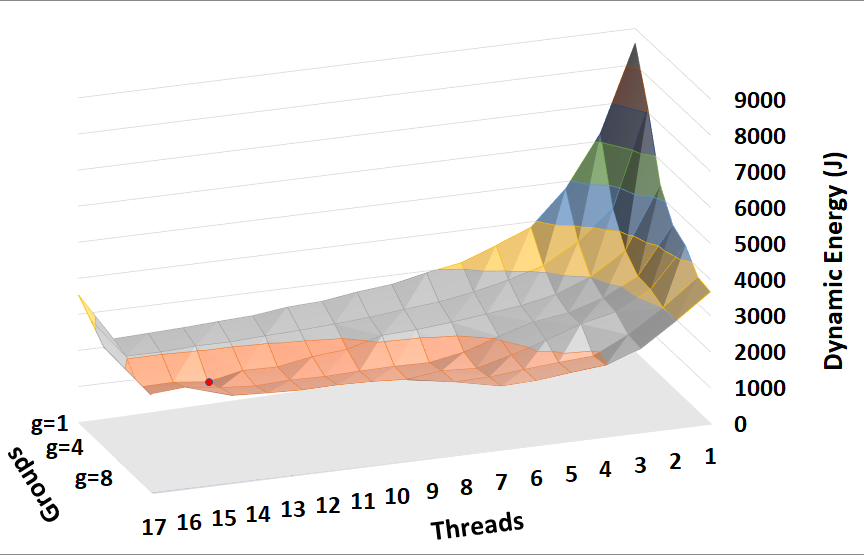
All results in this section are represented by a 3D surface represented by axes for performance or energy, number of threadgroups ($g$) and the number of threads in each threadgroup, $t$. The location of the minimum in the surface is shown by the red dot.

Figure 16a shows the results of PFFTTG using FFTW3.3.7 on S4 for matrix dimension N=30976. The area with minimum execution time is located in the figure in the region containing {4,7,8} threadgroups with 10 threads in each group. The minimum is achieved for the combination ($g,t$)=(7,10) with the execution time of 8 seconds. The speedup is around 100% in comparison with the best combination of threads for one group ($g,t$)=(1,10) where the execution time is 16 seconds.

(a)

(b)

Figure 16: (a). Performance profile of FFTW PFFTTG for different ($g$,$t$) configurations on S4 for workload size, N=30976. (b). Performance profile of FFTW PFFTTG for different ($g$,$t$) configurations on S3 for workload size, N=17728. Red dot represents the minimum.

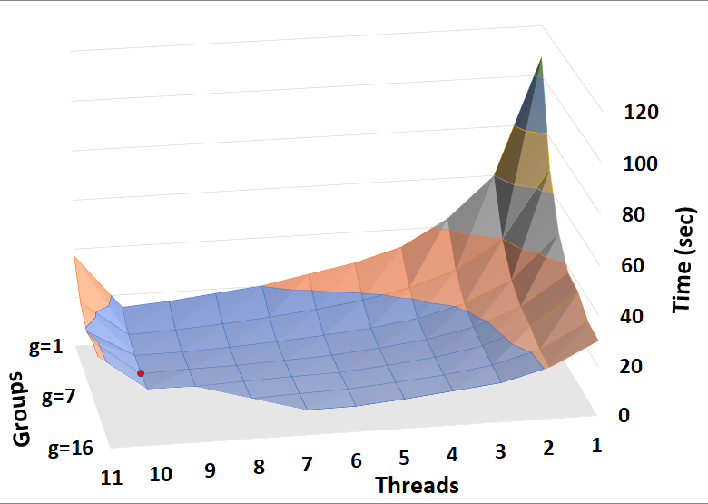
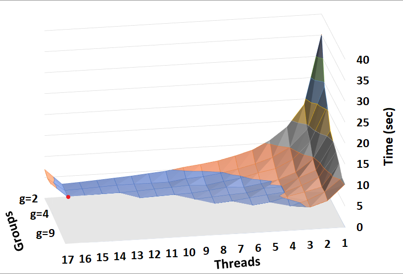
Figure 16b presents the results of PFFTTG using FFTW3.3.7 on S3 for the matrix dimension N=17728. The minimum is centred around number of threadsgroups equal to {4,7,8}. The minimum is achieved for the combination, ($g,t$)=(4,16). The performance improvement is 80% in comparison with ($g,t$)=(1,72), which is the best combination for one group.

7.2.3 Energy Optimization on a Single Socket Multicore CPU

Figure 17: Dynamic energy consumption of PFFTTG employing FFTW for different ($g$,$t$) configurations on S1.

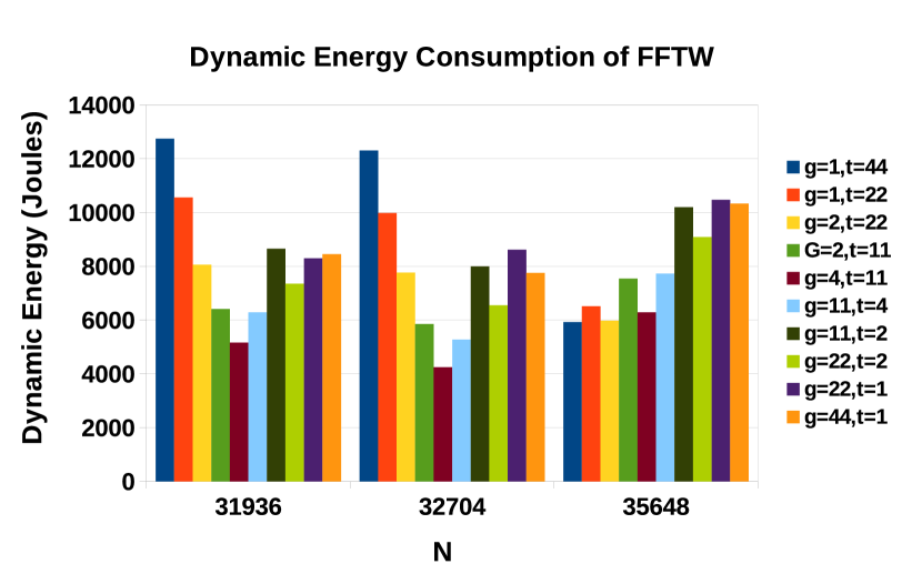
Figure 17 shows the dynamic energy comparision for PFFTTG employing FFTW between base and best combinations for workload sizes, 31936, 32704, and 35648 on a single-socket CPU (S1). The best combination ($g,t$)=(4,11) is the same for workload sizes, 31936 and 32704. The reductions in dynamic energy consumption in comparison with the base combination, ($g,t$)=(1,44), are 41% and 65%. For workload size 35648, the base combination is the best and outperforms the next best combination ($g,t$)=(2,22) by 5%. For Intel MKL FFT, the base combination, ($g$,$t$)=(1,44), is the best.

7.2.4 Energy Optimization on a Dual-socket Multicore CPU

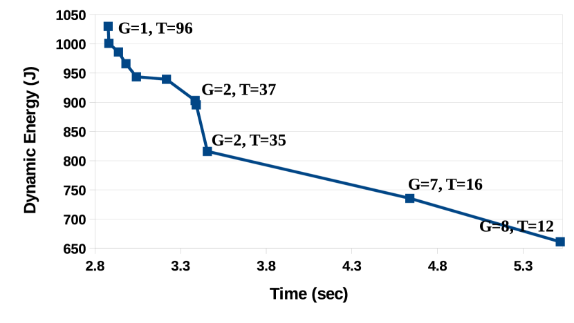
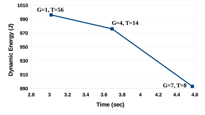
Figures 18a, 18b show the results for PFFTTG employing FFTW on S4 for matrix sizes equal to N=30464 and N=32192. The minimum for dynamic energy is located in {4,7,8} threadgroups with 14 threads in each threadgroup for workload size (N=32192) and 12 threads in each threadgroup for workload size 30464. The minimum for the workload size 30464 is achieved for the combination, ($g,t$)=(8,12). The dynamic energy consumption for this combination is 661 Joules. The energy saving is around 30% in comparison with the best combination of threads for one group ($g,t$)=(1,45) whose dynamic energy consumption is 918 Joules. The minimum for the workload size (N=32192) is achieved for the combination, ($g,t$)=(4,14). The saving is around 35% in comparison with ($g,t$)=(1,16) where dynamic energy is 2197 Joules.

(a)

(b)

Figure 18: (a). Energy profile of FFTW PFFTTG for different ($g$,$t$) configurations on S4 for workload size N=30464. (b). Energy profile of FFTW PFFTTG for different ($g$,$t$) configurations on S4 for workload size N=32192. Red dot represents the minimum.

7.3 Bi-Objective Optimization for Performance and Dynamic Energy

7.3.1 Single Socket Multicore CPU

(a)

(b)

Figure 19: (a). Pareto-optimal front of Intel MKL DGEMM PMMTG application on S1 for workload size N=32768. (b). Pareto-optimal front of Intel MKL FFT PFFTTG on S1 for workload size N=31744.

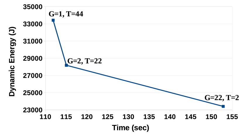
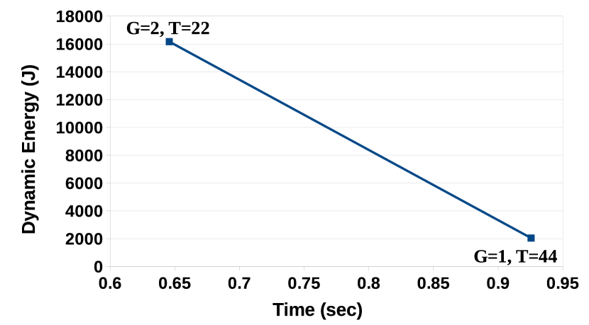
Figure 19a shows the globally Pareto-optimal front for PMMTG employing Intel MKL DGEMM on S1 for workload size 32768. Optimizing for dynamic energy consumption alone degrades performance by 27%, and optimizing for performance alone increases dynamic energy consumption by 30%. The average and maximum sizes of the Pareto-optimal fronts for Intel MKL DGEMM are (2.3,3).

Figure 19b shows the globally Pareto-optimal front for PFFTTG based on Intel MKL FFT on S1 for workload size 31744. There are two globally Pareto-optimal solutions. Optimizing for dynamic energy consumption alone degrades performance by around 31%, and optimizing for performance alone increases dynamic energy consumption by 87%. The average and maximum sizes of the Pareto-optimal fronts for Intel MKL FFT are (2.6,3).

No bi-objective trade-offs were observed for FFTW and OpenBLAS applications. We will investigate two lines of research in our future work. One is the influence of workload distribution; The other is the absence of bi-objective trade-offs for open-source packages such as FFTW and OpenBLAS using a dynamic energy predictive model.

7.3.2 Dual-socket Multicore CPUs

In this section, we will focus on bi-objective optimization on dual-socket CPUs, S2 and S4.

(a)

(b)

Figure 20: (a). Pareto-optimal front of FFTW PFFTTG on S4 for workload size, N=30464. (b). Pareto-optimal front of Intel MKL FFT PFFTTG on S4 for workload size, N=22208.

Figures 20a shows the globally Pareto-optimal fronts for PFFTTG FFTW on S4 for workload size, N=30464. The maximum number of globally Pareto-optimal solutions is 11. The optimization for dynamic energy consumption alone degrades performance by 49%, and optimizing for performance alone increases dynamic energy consumption by 35%.

Figure 20b shows the globally Pareto-optimal front for PFFTTG employing Intel MKL FFT on S2 for workload size, N=22208. Optimizing for dynamic energy consumption alone degrades performance by 33%, and optimizing for performance alone increases dynamic energy consumption by 10%. The average and maximum sizes of the Pareto-optimal fronts for FFTW and Intel MKL FFT are (3,11) and (2.7, 3).

(a)

(b)

Figure 21: (a). Pareto-optimal front of Intel MKL DGEMM PMMTG application on S2 for workload size, N=17408. (b). Pareto-optimal front of OpenBLAS DGEMM PMMTG application on S2 for workload size, N=17408.

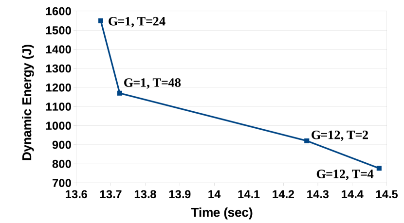
Figure 21a shows the globally Pareto-optimal front for PMMTG employing Intel MKL DGEMM on S2 for workload size, N=17408. Optimizing for dynamic energy consumption alone degrades performance by 5.5%, and optimizing for performance alone increases dynamic energy consumption by 50.7%. The average and maximum sizes of the Pareto-optimal fronts are (1.8, 4).

Figure 21b shows the globally Pareto-optimal front for PMMTG based on OpenBLAS DGEMM on S2 for workload size, N=17408. There are six globally Pareto-optimal solutions. Optimizing for dynamic energy consumption alone degrades performance by around 5%, and optimizing for performance alone increases dynamic energy consumption by 20%. The average and maximum sizes of the Pareto-optimal fronts are 2.4 and 5.

The execution time of building the four dimensional discrete graph with performance and dynamic energy as two objectives and the two decision variables can be cost-prohibitive for its employment in dynamic schedulers and self-adaptable data-parallel applications. We will explore approaches to reduce this time in our future work.

7.4 Analysis Using Performance and Dynamic Energy Models

In this section, we propose a qualitative dynamic energy model employing performance monitoring counters (PMCs) as parameters. The model reveals the cause behind the energy nonproportionality in modern multicore CPUs. The model along with the execution time of the application is used to analyze the Pareto-optimal front determined by our solution method on a dual-socket multicore platform.

PMCs are special-purpose registers provided in modern microprocessors to store the counts of software and hardware activities. The acronym PMCs is used to refer to software events, which are pure kernel-level counters such as page-faults, context-switches, etc. as well as micro-architectural events originating from the processor and its performance monitoring unit called the hardware events such as cache-misses, branch-instructions, etc. Software energy predictive models based on PMCs is one of the leading methods of measurement of energy consumption of an application [51].

The experimental platform S2 and the application OpenBLAS-DGEMM is employed for the analysis. Likwid tool [52] is used to obtain the PMCs. On this platform, it offers 164 PMCs, which are divided into 28 groups (L2CACHE, L3CACHE, NUMA, etc.). The groups are listed in the supplemental. All the PMCs for each workload size executed using different application configurations, (#threadgroups (g), #threads_per_group (t)) are collected. Each PMC value is the average for all the 24 physical cores. We analyzed the data to identify the major performance groups, which are highly correlated with the dynamic energy consumption. The highest correlation is contained in the data provided by TLB_DATA performance group. This group provides data activity, such as load miss rate, store miss rate and walk page duration, in L1 data translation lookaside buffer (dTLB), a small specialized cache of recent page address translations. If a dTLB miss occurs, the OS goes through the page tables. If there is a miss from the page walk, a page fault occurs resulting in the OS retrieving the corresponding page from memory. The duration of the page walk has the highest positive correlation with dynamic energy consumption based on our experiments.

(a)

(b)

Figure 22: (a). Measured (left) and predicted (right) dynamic energy consumption of OpenBLAS DGEMM on S2 for workload size, N=16384. (b). Measured (left) and predicted (right) dynamic energy consumption of OpenBLAS DGEMM on S2 for workload size, N=17408.

TABLE II: L1 dTLB PMC data for size 16384

Combination (g, t)	Dynamic Energy (J)	Time (sec)	L1 dTLB load miss duration (Cyc)	L1 dTLB store miss duration (Cyc)
(1,48)	824.2743	14.112	108.373	124.326
(4,12)	740.0211	14.177	113.515	105.363
(8,6)	729.1005	14.244	104.564	89.3753
(2,24)	802.6687	14.314	105.328	82.5185
(16,3)	750.6159	14.615	100.924	90.2733
(3,16)	631.3098	14.772	97.9180	76.1889
(6,8)	667.4856	14.818	96.8957	58.0210
(12,4)	528.0411	15.057	97.0492	52.8966
(24,2)	1352.141	15.875	100.106	82.7514
(48,1)	1719.012	18.685	111.902	85.9282

TABLE III: L1 dTLB PMC data for size 17408

Combination (g, t)	Dynamic Energy (J)	Time (sec)	L1 dTLB load miss duration (Cyc)	L1 dTLB store miss duration (Cyc)
(4,12)	1320.0702	16.2478	105.961	122.191
(1,48)	1271.5506	16.3034	99.5398	63.7090
(8,6)	1266.3294	16.3166	95.7896	58.9096
(2,24)	1287.6882	16.4498	98.2180	74.6859
(16,3)	1250.5616	16.6824	95.2988	58.3551
(6,8)	1130.2412	16.9668	93.4336	47.9097
(3,16)	1052.0283	17.0187	90.5275	45.7483
(24,2)	1824.5795	18.0755	106.804	55.5686
(12,4)	1795.7680	20.5520	93.6595	46.5541
(48,1)	2164.1212	20.9868	96.6999	71.4943

Non-negative multivariate regression is employed to construct our model of dynamic energy consumption based on the PMC data from dTLB. The model is shown below:

$$E_{dynamic}=\beta_{1}\times T+\beta_{2}\times L+\beta_{3}\times S$$ (1)

where $\beta_{1}$ is the average CPU utilization, $\beta_{2}$ and $\beta_{3}$ are the regression coefficients for the PMC data. $T$ is the execution time of the application, $L$ is the time of page walk caused by load miss and $S$ is the time of page walk caused by store miss in dTLB. The coefficients of the model ({$\beta_{1},\beta_{2},\beta_{3}$}) are forced to be non-negative to avoid erroneous cases where large values for them gives rise to negative dynamic energy consumption prediction violating the fundamental energy conservation law of computing.

To test this model, we use two workload sizes 16384 and 17408. The PMC data that is obtained for these sizes and that is used to train the model is shown in the tables II and III. The rows of the tables are sorted in increasing order of time. The blue colour in the tables shows the rows that are in the Pareto-optimal front. The time of page walk (last two columns, 4 and 5) is measured in cycles. As can be seen from the tables, the dynamic energy decreases as the number of cycles decreases.There is however a trade-off between the execution time of application and the page walk time. For a Pareto-optimal solution, a long execution time corresponds to smaller number of load and store cycles and thereby less dynamic energy consumption.

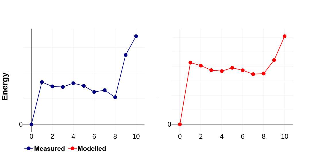
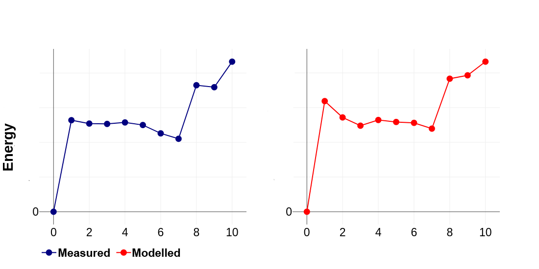
Two dynamic energy models for the workload sizes 16384 (Table II) and 17408 (Table III) were constructed. The coefficients for the workload size 16384 are {$\beta_{1}=253.680,\beta_{2}=39.536,\beta_{3}=13.647$}. The coefficients for the workload size 17408 are {$\beta_{1}=137.953,\beta_{2}=12.564,\beta_{3}=3.835$}. We then predict the dynamic energy consumption using the model and compare with the dynamic energy measured using HCLWattsUp. The Figures 22a and 22b illustrate the comparison. The $x$ axis represents the number of a row in the Tables II, III. The modeled dynamic energy demonstrates the same trend as the measured dynamic energy using HCLWattsUp.

TLB activity has been the focus of research in [53, 54, 55] where the authors state that the address translation using the TLB consumes as much as 16% of the chip power on some processors. The authors propose different strategies to improve the reuse of TLB caches. Our solution method employing threadgroups (or grouping using multithreaded kernels) allows to fill the page tables more evenly and reduce the duration of page walk resulting in less dynamic energy consumption.

To summarize, our proposed dynamic model based on parameters reflecting TLB activity (the duration of page walk) shows that the energy nonproportionality on our experimental platforms for the data-parallel applications is due to the activity of the data translation lookaside buffer (dTLB), which is disproportionately energy expensive. This finding may encourage the chip design architects to investigate and remove the nonproportionality in these platforms. There may be other causes behind the lack of energy proportionality as the range of applications and platforms is broadened that we would explore in our future research.

8 Conclusion

Energy proportionality is the key design goal followed by architects of modern multicore CPUs. One of its implications is that optimization of an application for performance will also optimize it for energy. However, due to the inherent complexities of resource contention for shared on-chip resources, NUMA, and dynamic power management in multicore CPUs, state-of-the-art application-level optimization methods for performance and energy [3, 4, 5, 21], demonstrate that the functional relationships between performance and workload size and between dynamic energy and workload size for real-life data-parallel applications have complex (non-linear) properties and show that workload distribution has become an important decision variable.

This motivated us to explore in-depth the influence of three-dimensional decision variable space on bi-objective optimization of applications for performance and energy on multicore CPUs. The three decision variables are: a). The number of identical multithreaded kernels (threadgroups) involved in the parallel execution of an application; b). The number of threads in each threadgroup; and c). The workload distribution between the threadgroups. We focused exclusively on the first two decision variables in this work.

By experimenting with these decision variables, we discovered that energy proportionality does not hold true for modern multicore CPUs. Based on this finding, we proposed the first application-level optimization method for bi-objective optimization of multithreaded data-parallel applications for performance and energy on a single multicore CPU. The method uses two decision variables, the number of identical multithreaded kernels (threadgroups) and the number of threads in each threadgroup. A given workload is partitioned equally between the threadgroups.

We demonstrated our method using four highly optimized multithreaded data-parallel applications, 2D fast Fourier transform based on FFTW and Intel MKL, and dense matrix-matrix multiplication written using Openblas DGEMM and Intel MKL, on four modern multicore CPUs one of which is a single socket multicore CPU and the other three dual-socket with increasing number of physical cores per socket. We showed in particular that optimizing for performance alone results in significant increase in dynamic energy consumption whereas optimizing for dynamic energy alone results in considerable performance degradation and that our method determined good number of globally Pareto-optimal solutions.

Finally, we proposed a qualitative dynamic energy model employing performance monitoring counters (PMCs) as parameters, which we used to explain the Pareto-optimal solutions determined for modern multicore CPUs. The model showed that the energy nonproportionality on our experimental platforms for the two data-parallel applications is caused by disproportionately high energy consumption by the data translation lookaside buffer (dTLB) activity.

9 Supplementary Material

9.1 Rationale Behind Using Dynamic Energy Consumption Instead of Total Energy Consumption

There are two types of energy consumptions, static energy, and dynamic energy. We define the static energy consumption as the energy consumption of the platform without the given application execution. Dynamic energy consumption is calculated by subtracting this static energy consumption from the total energy consumption of the platform during the given application execution. The static energy consumption is calculated by multiplying the idle power of the platform (without application execution) with the execution time of the application. That is, if $P_{S}$ is the static power consumption of the platform, $E_{T}$ is the total energy consumption of the platform during the execution of an application, which takes $T_{E}$ seconds, then the dynamic energy $E_{D}$ can be calculated as,

$$E_{D}=E_{T}-(P_{S}\times T_{E})$$ (2)

We consider only the dynamic energy consumption in our work for reasons below:

1. Static energy consumption is a constant (or a inherent property) of a platform that can not be optimized. It does not depend on the application configuration.

2. Although static energy consumption is a major concern in embedded systems, it is becoming less compared to the dynamic energy consumption due to advancements in hardware architecture design in HPC systems.

3. We target applications and platforms where dynamic energy consumption is the dominating energy dissipator.

4. Finally, we believe its inclusion can underestimate the true worth of an optimization technique that minimizes the dynamic energy consumption. We elucidate using two examples from published results.

   • In our first example, consider a model that reports predicted and measured total energy consumption of a system to be 16500J and 18000J. It would report the prediction error to be 8.3%. If it is known that the static energy consumption of the system is 9000J, then the actual prediction error (based on dynamic energy consumptions only) would be 16.6% instead.

   • In our second example, consider two different energy prediction models ($M_{A}$ and $M_{B}$) with same prediction errors of 5% for an application execution on two different machines ($A$ and $B$) with same total energy consumption of 10000J. One would consider both the models to be equally accurate. But supposing it is known that the dynamic energy proportions for the machines are 30% and 60%. Now, the true prediction errors (using dynamic energy consumptions only) for the models would be 16.6% and 8.3%. Therefore, the second model $M_{B}$ should be considered more accurate than the first.

9.2 Shared Memory Implementations of PMMTG Algorithms

The shared memory implementations of PMMTG algorithms using Intel MKL and OpenBLAS are described here. The inputs to an implementation are: a). Matrices A, B, and C of sizes $N\times N$; b). Constants $\alpha$ and $\beta$; c) The number of abstract processors (groups), $\{P_{1},\cdots,P_{p}\}$; d). The number of threads in each abstract processor (group) represented by $t$. The output matrix, C, contains the matrix product. Each abstract processor is a group of $t$ threads.

The implementations using Intel MKL differ from those using OpenBLAS. In Intel MKL, the matrix-matrix computation specific to a partition is computed using an OpenMP parallel region with $t$ threads whereas the same is computed in OpenBLAS using a pthread.

9.2.1 Intel MKL implementation of PMMTG-V

Figure 23 shows the implementation of PMMTG-V using Intel MKL.

⬇

1int row;

2#pragma omp parallel for num_threads(p*t)

3for (row = 0; row < N; row++) {

4 memcpy(&B1[row*(N/p)], &B[row*N],

5 (N/p)*sizeof(double));

6 …

7 memcpy(&Bp[row*(N/p)], &B[(p-1)*(N/p)+row*N],

8 (N/p)*sizeof(double));

9 memcpy(&C1[row*(N/p)], &C[row*N],

10 (N/p)*sizeof(double));

11 …

12 memcpy(&Cp[row*(N/p)], &C[(p-1)*(N/p)+row*N],

13 (N/p)*sizeof(double));

14}

15

16#pragma omp parallel sections num_threads(p*t)

17{

18 #pragma omp section // processor 1

19 {

20 mkl_set_num_threads_local(t);

21 cblas_dgemm(CblasRowMajor, CblasNoTrans,

22 CblasNoTrans, N, N/p, N, alpha, A, N,

23 B1, N/p, beta, C1, N/p);

24 }

25 …

26 #pragma omp section // processor p

27 {

28 mkl_set_num_threads_local(t);

29 cblas_dgemm(CblasRowMajor, CblasNoTrans,

30 CblasNoTrans, N, N/p, N, alpha, A, N,

31 Bp, N/p, beta, Cp, N/p);

32 }

33}

34

35#pragma omp parallel for num_threads(p*t)

36for (row = 0; row < N; row++)

37{

38 memcpy(&B[row*N], &B1[row*(N/p)],

39 (N/p)*sizeof(double));

40 …

41 memcpy(&B[(p-1)*(N/p)+row*N], &Bp[row*(N/p)],

42 (N/p)*sizeof(double));

43 memcpy(&C[row*N], &C1[row*(N/p)],

44 (N/p)*sizeof(double));

45 …

46 memcpy(&C[(p-1)*(N/p)+row*N], &Cp[row*(N/p)],

47 (N/p)*sizeof(double));

48}

Figure 23: Intel MKL implementation of PMMTG-V employing $p$ abstract processors of $t$ threads each.

9.2.2 OpenBLAS implementation of PMMTG-V

Figure 24 shows the implementation of PMMTG-V using OpenBLAS.

⬇

1void *dgemm(void *input) {

2 int i = *(int*)input;

3 openblas_set_num_threads(t);

4 goto_set_num_threads(t);

5 omp_set_num_threads(t);

6 if (i == 1)

7 {

8 cblas_dgemm(CblasRowMajor, CblasNoTrans,

9 CblasNoTrans, N, N/p, N, alpha, A, N,

10 B1, N/p, beta, C1, N/p);

11 }

12 …

13 if (i == p)

14 {

15 cblas_dgemm(CblasRowMajor, CblasNoTrans,

16 CblasNoTrans, N, N/p, N, alpha, A, N,

17 Bp, N/p, beta, Cp, N/p);

18 }

19}

20

21int main() {

22 int row;

23#pragma omp parallel for num_threads(p*t)

24 for (row = 0; row < N; row++) {

25 memcpy(&B1[row*(N/p)], &B[row*N],

26 (N/p)*sizeof(double));

27 …

28 memcpy(&Bp[row*(N/p)], &B[(p-1)*(N/p)+row*N],

29 (N/p)*sizeof(double));

30 memcpy(&C1[row*(N/p)], &C[row*N],

31 (N/p)*sizeof(double));

32 …

33 memcpy(&Cp[row*(N/p)], &C[(p-1)*(N/p)+row*N],

34 (N/p)*sizeof(double));

35 }

36

37 pthread_t t1, …, tp;

38 int i1 = 1, …, ip = p;

39 pthread_create(&t1, NULL, dgemm, &i1);

40 …

41 pthread_create(&tp, NULL, dgemm, &ip);

42 pthread_join(tp, NULL);

43 …

44 pthread_join(t1, NULL);

45

46#pragma omp parallel for num_threads(p*t)

47 for (row = 0; row < N; row++)

48 {

49 memcpy(&B[row*N], &B1[row*(N/p)],

50 (N/p)*sizeof(double));

51 …

52 memcpy(&B[(p-1)*(N/p)+row*N], &Bp[row*(N/p)],

53 (N/p)*sizeof(double));

54 memcpy(&C[row*N], &C1[row*(N/p)],

55 (N/p)*sizeof(double));

56 …

57 memcpy(&C[(p-1)*(N/p)+row*N], &Cp[row*(N/p)],

58 (N/p)*sizeof(double));

59 }

60}

Figure 24: OpenBLAS implementation of PMMTG-V employing $p$ abstract processors of $t$ threads each.

9.2.3 Intel MKL implementation of PMMTG-S

Figure 25 shows the implementation of PMMTG-S using Intel MKL.

⬇

1#pragma omp parallel for num_threads(4*t)

2for (row = 0; row < (N/2); row++) {

3 memcpy(&A11[row*(N/2)], &A[row*N],

4 (N/2)*sizeof(double));

5 memcpy(&A22[row*(N/2)], &A[N*(N/2)+(N/2)+row*N],

6 (N/2)*sizeof(double));

7 …

8 memcpy(&B11[row*(N/2)], &B[row*N],

9 (N/2)*sizeof(double));

10 memcpy(&B22[row*(N/2)], &B[N*(N/2)+(N/2)+row*N],

11 (N/2)*sizeof(double));

12 …

13 memcpy(&C11[row*(N/2)], &C[row*N],

14 (N/2)*sizeof(double));

15 memcpy(&C22[row*(N/2)], &C[N*(N/2)+(N/2)+row*N],

16 (N/2)*sizeof(double));

17 …

18}

19

20#pragma omp parallel sections num_threads(4)

21{

22 #pragma omp section // processor 1

23 {

24 mkl_set_num_threads_local(t);

25 cblas_dgemm(CblasRowMajor, CblasNoTrans,

26 CblasNoTrans, N/2, N/2, N/2, alpha, A11, N/2,

27 B11, N/2, beta0, C11, N/2);

28 cblas_dgemm(CblasRowMajor, CblasNoTrans,

29 CblasNoTrans, N/2, N/2, N/2, alpha, A12, N/2,

30 B21, N/2, beta1, C11, N/2);

31 }

32 …

33 #pragma omp section // processor 4

34 {

35 mkl_set_num_threads_local(t);

36 cblas_dgemm(CblasRowMajor, CblasNoTrans,

37 CblasNoTrans, N/2, N/2, N/2, alpha, A21, N/2,

38 B12, N/2, beta0, C22, N/2);

39 cblas_dgemm(CblasRowMajor, CblasNoTrans,

40 CblasNoTrans, N/2, N/2, N/2, alpha, A22, N/2,

41 B22, N/2, beta1, C22, N/2);

42 }

43}

44

45#pragma omp parallel for num_threads(4*t)

46for (row = 0; row < (N/2); row++) {

47 memcpy(&A[row*N], &A11[row*(N/2)],

48 (N/2)*sizeof(double));

49 memcpy(&A[N*(N/2)+(N/2)+row*N], &A22[row*(N/2)],

50 (N/2)*sizeof(double));

51 …

52 memcpy(&B[row*N], &B11[row*(N/2)],

53 (N/2)*sizeof(double));

54 memcpy(&B[N*(N/2)+(N/2)+row*N], &B22[row*(N/2)],

55 (N/2)*sizeof(double));

56 …

57 memcpy(&C[row*N], &C11[row*(N/2)],

58 (N/2)*sizeof(double));

59 memcpy(&C[N*(N/2)+(N/2)+row*N], &C22[row*(N/2)],

60 (N/2)*sizeof(double));

61 …

62}

Figure 25: Intel MKL implementation of PMMTG-S employing 4 abstract processors of $t$ threads each and arranged in a 2 $\times$ 2 grid.

9.2.4 OpenBLAS implementation of PMMTG-S

Figure 26 shows the implementation of PMMTG-S using OpenBLAS.

⬇

1void *dgemm(void *input){

2 int i = *(int*)input;

3 openblas_set_num_threads(t);

4 goto_set_num_threads(t);

5 omp_set_num_threads(t);

6 if (i == 1){

7 cblas_dgemm(CblasRowMajor, CblasNoTrans,

8 CblasNoTrans, N/2, N/2, N/2, alpha, A11, N/2,

9 B11, N/2, beta0, C11, N/2);

10 cblas_dgemm(CblasRowMajor, CblasNoTrans,

11 CblasNoTrans, N/2, N/2, N/2, alpha, A12, N/2,

12 B21, N/2, beta1, C11, N/2);

13 }

14 …

15 if (i == 4){

16 cblas_dgemm(CblasRowMajor, CblasNoTrans,

17 CblasNoTrans, N/2, N/2, N/2, alpha, A21, N/2,

18 B12, N/2, beta0, C22, N/2);

19 cblas_dgemm(CblasRowMajor, CblasNoTrans,

20 CblasNoTrans, N/2, N/2, N/2, alpha, A22, N/2,

21 B22, N/2, beta1, C22, N/2);

22 }

23}

24int main(){

25 int row;

26#pragma omp parallel for num_threads(4*t)

27 for (row = 0; row < (N/2); row++) {

28 memcpy(&A11[row*(N/2)], &A[row*N],

29 (N/2)*sizeof(double));

30 memcpy(&A22[row*(N/2)], &A[N*(N/2)+(N/2)+row*N],

31 (N/2)*sizeof(double));

32 …

33 memcpy(&B11[row*(N/2)], &B[row*N],

34 (N/2)*sizeof(double));

35 memcpy(&B22[row*(N/2)], &B[N*(N/2)+(N/2)+row*N],

36 (N/2)*sizeof(double));

37 …

38 memcpy(&C11[row*(N/2)], &C[row*N],

39 (N/2)*sizeof(double));

40 memcpy(&C22[row*(N/2)], &C[N*(N/2)+(N/2)+row*N],

41 (N/2)*sizeof(double));

42 …

43 }

44

45 pthread_t t1, …, t4;

46 int i1 = 1, …, i4 = 4;

47 pthread_create(&t1, NULL, dgemm, &i1);

48 …

49 pthread_create(&t4, NULL, dgemm, &i4);

50 pthread_join(t4, NULL);

51 …

52 pthread_join(t1, NULL);

53

54#pragma omp parallel for num_threads(4*t)

55 for (row = 0; row < (N/2); row++) {

56 memcpy(&A[row*N], &A11[row*(N/2)],

57 (N/2)*sizeof(double));

58 memcpy(&A[N*(N/2)+(N/2)+row*N], &A22[row*(N/2)],

59 (N/2)*sizeof(double));

60 …

61 memcpy(&B[row*N], &B11[row*(N/2)],

62 (N/2)*sizeof(double));

63 memcpy(&B[N*(N/2)+(N/2)+row*N], &B22[row*(N/2)],

64 (N/2)*sizeof(double));

65 …

66 memcpy(&C[row*N], &C11[row*(N/2)],

67 (N/2)*sizeof(double));

68 memcpy(&C[N*(N/2)+(N/2)+row*N], &C22[row*(N/2)],

69 (N/2)*sizeof(double));

70 …

71 }

72}

Figure 26: OpenBLAS implementation of PMMTG-S employing 4 abstract processors of $t$ threads each and arranged in a 2 $\times$ 2 grid.

9.2.5 Intel MKL implementation of PMMTG-H

Figure 27 shows the implementation of PMMTG-H using Intel MKL.

⬇

1int row;

2#pragma omp parallel for num_threads(p*t)

3for (row = 0; row < N/p; row++) {

4 memcpy(&A1[row*N], &A[row*N],

5 N*sizeof(double));

6 …

7 memcpy(&Ap[row*N], &A[(p-1)*N*(N/p)+row*N],

8 N*sizeof(double));

9 memcpy(&C1[row*N], &C[row*N],

10 N*sizeof(double));

11 …

12 memcpy(&Cp[row*N], &C[(p-1)*N*(N/p)+row*N],

13 N*sizeof(double));

14}

15

16#pragma omp parallel sections num_threads(p*t)

17{

18 #pragma omp section // processor 1

19 {

20 mkl_set_num_threads_local(t);

21 cblas_dgemm(CblasRowMajor, CblasNoTrans,

22 CblasNoTrans, N/p, N, N, alpha, A1, N,

23 B, N, beta, C1, N);

24 }

25 …

26 #pragma omp section // processor p

27 {

28 mkl_set_num_threads_local(t);

29 cblas_dgemm(CblasRowMajor, CblasNoTrans,

30 CblasNoTrans, N/p, N, N, alpha, Ap, N,

31 B, N, beta, Cp, N);

32 }

33}

34

35#pragma omp parallel for num_threads(p*t)

36for (row = 0; row < N/p; row++)

37{

38 memcpy(&A[row*N], &A1[row*N],

39 N*sizeof(double));

40 …

41 memcpy(&A[(p-1)*N*(N/p)+row*N], &Ap[row*N],

42 N*sizeof(double));

43 memcpy(&C[row*N], &C1[row*N],

44 N*sizeof(double));

45 …

46 memcpy(&C[(p-1)*N*(N/p)+row*N], &Cp[row*N],

47 N*sizeof(double));

48}

Figure 27: Intel MKL implementation of PMMTG-H employing $p$ abstract processors of $t$ threads each.

9.3 Shared Memory Implementations of PFFT Algorithms

The inputs to an implementation are: a). Signal matrix $\mathcal{M}$ of size $N\times N$; b). The number of abstract processors (groups) $p$, $\{P_{1},\cdots,P_{p}\}$; c). The number of threads in each abstract processor (group) represented by $t$. The output is the transformed signal matrix $\mathcal{M}$ (considering that we are performing in-place FFT). Each abstract processor is a group of $t$ threads.

The implementations using Intel MKL differ from those using FFTW. In FFTW, only plan execution (fftw_plan_many_dft) and plan destruction (fftw_destroy_plan) are thread-safe and called be called in an OpenMP parallel region.

9.3.1 Intel MKL implementation of PFFTTG-H

Figure 28 shows the implementation of PFFTTG-H using Intel MKL.

⬇

1

2void fftw1d(const int sign, const int m,

3 const int n, fftw_complex* X,fftw_complex* Y)

4{

5 int rank = 1, howmany = m;

6 int s[] = {n};

7 int idist = n, odist = n;

8 int istride = 1, ostride = 1;

9 int *inembed = s, *onembed = s;

10 fftw_plan my_plan = fftw_plan_many_dft(

11 rank, s, howmany,

12 X, inembed, istride, idist,

13 Y, onembed, ostride, odist,

14 sign, FFTW_ESTIMATE);

15 fftw_execute(my_plan);

16 fftw_destroy_plan(my_plan);

17 return;

18}

19

20int

21fftw2d(const int sign, const int N, const int p,

22 const unsigned int nt, const unsigned int blockSize,

23 fftw_complex* X)

24{

25#pragma omp parallel sections num_threads(p)

26{

27 #pragma omp section

28 {

29 fftw1d(sign, N/p, N, X, X);

30 }

31…

32 #pragma omp section

33 {

34 fftw1d(sign, N-(p-1)*(N/p), N,

35 &X[(p-1)*(N/p)*N], &X[(p-1)*(N/p)*N]);

36 }

37}

38

39 hcl_transpose_block(X, 0, N, N, nt, blockSize);

40

41#pragma omp parallel sections num_threads(p)

42{

43 #pragma omp section

44 {

45 fftw1d(sign, N/p, N, X, X);

46 }

47…

48 #pragma omp section

49 {

50 fftw1d(sign, N-(p-1)*(N/p), N,

51 &X[(p-1)*(N/p)*N], &X[(p-1)*(N/p)*N]);

52 }

53}

54

55 hcl_transpose_block(X, 0, N, N, nt, blockSize);

56}

Figure 28: Intel MKL implementation of PFFTTG-H employing $p$ abstract processors of $t$ threads each.

9.4 Transpose Routine Invoked in PFFT Algorithms

The routine, hcl_transpose_block, shown in the Figure 29 performs in-place transpose of a complex 2D square matrix of size $n\times n$. We use a block size of 64 in our experiments as it is found to be optimal.

⬇

1void hcl_transpose_scalar_block(fftw_complex* X1,

2 fftw_complex* X2, const int i, const int j,

3 const int N, const int block_size)

4{

5 int p, q;

6 for (p = 0; p < min(N-i,block_size); p++) {

7 for (q = 0; q < min(N-j,block_size); q++) {

8 int index1 = i*N+j + p*N+q;

9 int index2 = j*N+i + q*N+p;

10

11 if (index1 >= index2)

12 continue;

13

14 double tmpr = X1[p*N+q][0];

15 double tmpi = X1[p*N+q][1];

16 X1[p*N+q][0] = X2[q*N+p][0];

17 X1[p*N+q][1] = X2[q*N+p][1];

18 X2[q*N+p][0] = tmpr;

19 X2[q*N+p][1] = tmpi;

20 }

21 }

22}

23

24void hcl_transpose_block(fftw_complex* X, const int start,

25 const int end, const int n,

26 const unsigned int nt, const int block_size)

27{

28 int i, j;

29#pragma omp parallel for shared(X) private(i, j) num_threads(nt)

30 for (i = 0; i < end; i += block_size) {

31 for (j = 0; j < end; j += block_size) {

32 hcl_transpose_scalar_block(

33 &X[start + i*N + j],

34 &X[start + j*N + i],

35 i, j, N, block_size);

36 }

37 }

38}

Figure 29: Transpose of square matrix of size $n\times n$ using blocking.

9.5 Application Programming Interface (API) for Measurements Using External Power Meter Interfaces (HCLWattsUp)

HCLServer01, HCLServer02 and HCLServer03 have a dedicated power meter installed between their input power sockets and wall A/C outlets. The power meter captures the total power consumption of the node. It has a data cable connected to the USB port of the node. A perl script collects the data from the power meter using the serial USB interface. The execution of this script is non-intrusive and consumes insignifcant power.

We use HCLWattsUp API function, which gathers the readings from the power meters to determine the average power and energy consumption during the execution of an application on a given platform. HCLWattsUp API can provide following four types of measures during the execution of an application:

• TIME—The execution time (seconds).

• DPOWER—The average dynamic power (watts).

• TENERGY—The total energy consumption (joules).

• DENERGY—The dynamic energy consumption (joules).

We confirm that the overhead due to the API is very minimal and does not have any noticeable influence on the main measurements. It is important to note that the power meter readings are only processed if the measure is not hcl::TIME. Therefore, for each measurement, we have two runs. One run for measuring the execution time. And the other for energy consumption. The following example illustrates the use of statistical methods to measure the dynamic energy consumption during the execution of an application.

The API is confined in the hcl namespace. Lines 10–12 construct the Wattsup object. The inputs to the constructor are the paths to the scripts and their arguments that read the USB serial devices containing the readings of the power meters.

The principal method of Wattsup class is execute. The inputs to this method are the type of measure, the path to the executable executablePath, the arguments to the executable executableArgs and the statistical thresholds (pIn) The outputs are the achieved statistical confidence pOut, the estimators, the sample mean (sampleMean) and the standard deviation (sd) calculated during the execution of the executable.

⬇

1#include <wattsup.hpp>

2int main(int argc, char** argv)

3{

4 std::string pathsToMeters[2] = {

5 ”/opt/powertools/bin/wattsup1”,

6 ”/opt/powertools/bin/wattsup2”};

7 std::string argsToMeters[2] = {

8 ”–interval=1”,

9 ”–interval=1”};

10 hcl::Wattsup wattsup(

11 2, pathsToMeters, argsToMeters

12 );

13 hcl::Precision pIn = {

14 maxRepeats, cl, maxElapsedTime, maxStdError

15 };

16 hcl::Precision pOut;

17 double sampleMean, sd;

18 int rc = wattsup.execute(

19 hcl::DENERGY, executablePath,

20 executableArgs, &pIn, &pOut,

21 &sampleMean, &sd

22 );

23 if (rc == 0)

24 std::cerr << ”Precision NOT achieved.\n”;

25 else

26 std::cout << ”Precision achieved.\n”;

27 std::cout << ”Max repetitions ”

28 << pOut.reps_max

29 << ”, Elasped time ”

30 << pOut.time_max_rep

31 << ”, Relative error ”

32 << pOut-eps-converted-to.pdf

33 << ”, Mean energy ”

34 << sampleMean

35 << ”, Standard Deviation ”

36 << sd

37 << std::endl;

38 exit(EXIT_SUCCESS);

39}

Figure 30: Example illustrating the use of HCLWattsUp API for measuring the dynamic energy consumption

The execute method repeatedly invokes the executable until one of the following conditions is satisfied:

• The maximum number of repetitions specified in $maxRepeats$ is exceeded.

• The sample mean is within $maxStdError$ percent of the confidence interval $cl$. The confidence interval of the mean is estimated using Student’s t-distribution.

• The maximum allowed time $maxElapsedTime$ specified in seconds has elapsed.

If any one of the conditions are not satisfied, then a return code of 0 is output suggesting that statistical confidence has not been achieved. If statistical confidence has been achieved, then the number of repetitions performed, time elapsed and the final relative standard error is returned in the output argument $pOut$. At the same time, the sample mean and standard deviation are returned. For our experiments, we use values of (1000, 95%, 2.5%, 3600) for the parameters ($maxRepeats,cl,maxStdError,maxElapsedTime$) respectively. Since we use Student’s t-distribution for the calculation of the confidence interval of the mean, we confirm specifically that the observations follow normal distribution by plotting the density of the observations using R tool.

9.6 Experimental Methodology to Determine the Sample Mean

We followed the methodology described below to make sure the experimental results are reliable:

• The server is fully reserved and dedicated to these experiments during their execution. We also made certain that there are no drastic fluctuations in the load due to abnormal events in the server by monitoring its load continuously for a week using the tool sar. Insignificant variation in the load was observed during this monitoring period suggesting normal and clean behaviour of the server.

• An application during its execution is bound to the physical cores using the numactl tool.

• To obtain a data point, the application is repeatedly executed until the sample mean lies in the 95% confidence interval with precision of 0.025 (2.5%). For this purpose, we use Student’s t-test assuming that the individual observations are independent and their population follows the normal distribution. We verify the validity of these assumptions using Pearson’s chi-squared test. When we mention a single number such as execution time (seconds) or floating-point performance (in MFLOPs or GFLOPs), we imply the sample mean determined using the Student’s t-test.

  The function $MeanUsingTtest$, shown in Algorithm 1, determines the sample mean for a data point. For each data point, the function repeatedly executes the application $app$ until one of the following three conditions is satisfied:

  1. The maximum number of repetitions ($maxReps$) is exceeded (Line 3).

  2. The sample mean falls in the confidence interval (or the precision of measurement $eps$ is achieved) (Lines 13-15).

  3. The elapsed time of the repetitions of application execution has exceeded the maximum time allowed ($maxT$ in seconds) (Lines 16-18).

  So, for each data point, the function $MeanUsingTtest$ returns the sample mean $mean$. The function $Measure$ measures the execution time using gettimeofday function.

• In our experiments, we set the minimum and maximum number of repetitions, $minReps$ and $maxReps$, to 15 and 100000. The values of $maxT$, $cl$, and $eps$ are 3600, 0.95, and 0.025. If the precision of measurement is not achieved before the completion of maximum number of repeats, we increase the number of repetitions and also the allowed maximum elapsed time. Therefore, we make sure that statistical confidence is achieved for all the data points that we use in our experiments.

Solution Method 1 Function determining the mean of an experimental run using Student’s t-test.

1:procedure MeanUsingTtest($app,minReps,maxReps,$ $maxT,cl,accuracy,$ $repsOut,clOut,etimeOut,epsOut,mean$)

2:

3:The application to execute, $app$

4:The minimum number of repetitions, $minReps\in\mathbb{Z}_{>0}$

5:The maximum number of repetitions, $maxReps\in\mathbb{Z}_{>0}$

6:The maximum time allowed for the application to run, $maxT\in\mathbb{R}_{>0}$

7:The required confidence level, $cl\in\mathbb{R}_{>0}$

8:The required accuracy, $eps\in\mathbb{R}_{>0}$

9:

10:The number of experimental runs actually made, $repsOut\in\mathbb{Z}_{>0}$

11:The confidence level achieved, $clOut\in\mathbb{R}_{>0}$

12:The accuracy achieved, $epsOut\in\mathbb{R}_{>0}$

13:The elapsed time, $etimeOut\in\mathbb{R}_{>0}$

14:The mean, $mean\in\mathbb{R}_{>0}$

15:

16:     $reps\leftarrow 0$; $stop\leftarrow 0$; $sum\leftarrow 0$; $etime\leftarrow 0$

17:     while ($reps<maxReps$) and ($!stop$) do

18:         $st\leftarrow{measure}(TIME)$

19:         ${Execute}(app)$

20:         $et\leftarrow{measure}(TIME)$

21:         $reps\leftarrow reps+1$

22:         $etime\leftarrow etime+et-st$

23:         $ObjArray[reps]\leftarrow et-st$

24:         $sum\leftarrow sum+ObjArray[reps]$

25:         if $reps>minReps$ then

26:              $clOut$ $\leftarrow$ fabs(gsl_cdf_tdist_Pinv($cl$, $reps-1$))                $\times$ gsl_stats_sd($ObjArray$, 1, $reps$)                / sqrt($reps$)

27:              if $clOut\times\frac{reps}{sum}<eps$ then

28:                  $stop\leftarrow 1$

29:              end if

30:              if $etime>maxT$ then

31:                  $stop\leftarrow 1$

32:              end if

33:         end if

34:     end while

35:     $repsOut\leftarrow reps$; $epsOut\leftarrow clOut\times\frac{reps}{sum}$

36:     $etimeOut\leftarrow etime$; $mean\leftarrow\frac{sum}{reps}$

37:end procedure

9.7 List of PMC groups Provided by Likwid

The list of PMC groups provided by Likwid tool [52] on HCLServer2 (S2) is shown in the Figure 31.

TABLE IV: Specification of the Intel multicore CPU platform, HCLServer2.

Technical Specifications	HCLServer2 (S2)
Processor	Intel Haswell E5-2670V3
OS	CentOS 7.2.1511
Core(s) per socket	12
Socket(s)	2
L1d cache, L1i cache	32 KB, 32 KB
L2 cache, L3 cache	256 KB, 30976 KB
Total main memory	64 GB
Power meter	WattsUp Pro

⬇

1$ likwid-perfctr -a

2

3 Group name Description

4———– —————————————-

5 BRANCH Branch prediction miss rate/ratio

6 CACHES Cache bandwidth in MBytes/s

7 CBOX CBOX related data and metrics

8 CLOCK Power and Energy consumption

9 DATA Load to store ratio

10 ENERGY Power and Energy consumption

11FALSE_SHARE False sharing

12 FLOPS_AVX Packed AVX MFLOP/s

13 HA Main memory bandwidth in MBytes/s seen

14 from Home agent

15 ICACHE Instruction cache miss rate/ratio

16 L2 L2 cache bandwidth in MBytes/s

17 L2CACHE L2 cache miss rate/ratio

18 L3 L3 cache bandwidth in MBytes/s

19 L3CACHE L3 cache miss rate/ratio

20 MEM Main memory bandwidth in MBytes/s

21 NUMA Local and remote memory accesses

22 QPI QPI Link Layer data

23 RECOVERY Recovery duration

24 SBOX Ring Transfer bandwidth

25 TLB_DATA L2 data TLB miss rate/ratio

26 TLB_INSTR L1 Instruction TLB miss rate/ratio

27 UOPS UOPs execution info

28 UOPS_EXEC UOPs execution

29 UOPS_ISSUE UOPs issueing

30UOPS_RETIRE UOPs retirement

31CYCLE_ACTIVITY Cycle Activities

Figure 31: List of PMC groups provided by Likwid tool on HCLServer02

References

- [1] L. A. Barroso and U. Hölzle, “The case for energy-proportional computing,” Computer, no. 12, pp. 33–37, 2007.
- [2] R. Sen and D. A. Wood, “Energy-proportional computing: A new definition,” Computer, vol. 50, no. 8, pp. 26–33, 2017.
- [3] A. Lastovetsky and R. Reddy, “New model-based methods and algorithms for performance and energy optimization of data parallel applications on homogeneous multicore clusters,” IEEE Transactions on Parallel and Distributed Systems, vol. 28, no. 4, pp. 1119–1133, April 2017.
- [4] R. R. Manumachu and A. Lastovetsky, “Bi-objective optimization of data-parallel applications on homogeneous multicore clusters for performance and energy,” IEEE Transactions on Computers, vol. 67, no. 2, pp. 160–177, 2018.
- [5] R. Reddy Manumachu and A. L. Lastovetsky, “Design of self-adaptable data parallel applications on multicore clusters automatically optimized for performance and energy through load distribution,” Concurrency and Computation: Practice and Experience, vol. 0, no. 0, p. e4958.
- [6] V. Petrucci, O. Loques, D. Mossé, R. Melhem, N. A. Gazala, and S. Gobriel, “Energy-efficient thread assignment optimization for heterogeneous multicore systems,” ACM Trans. Embed. Comput. Syst., vol. 14, no. 1, Jan. 2015.
- [7] Y. G. Kim, M. Kim, and S. W. Chung, “Enhancing energy efficiency of multimedia applications in heterogeneous mobile multi-core processors,” IEEE Transactions on Computers, vol. 66, no. 11, pp. 1878–1889, Nov 2017.
- [8] W. Wang, P. Mishra, and S. Ranka, “Dynamic cache reconfiguration and partitioning for energy optimization in real-time multi-core systems,” in 2011 48th ACM/EDAC/IEEE Design Automation Conference (DAC), June 2011, pp. 948–953.
- [9] G. Chen, K. Huang, J. Huang, and A. Knoll, “Cache partitioning and scheduling for energy optimization of real-time mpsocs,” in 2013 IEEE 24th International Conference on Application-Specific Systems, Architectures and Processors, June 2013, pp. 35–41.
- [10] S. Zhuravlev, J. C. Saez, S. Blagodurov, A. Fedorova, and M. Prieto, “Survey of scheduling techniques for addressing shared resources in multicore processors,” ACM Comput. Surv., vol. 45, no. 1, Dec. 2012.
- [11] J. Yang, X. Zhou, M. Chrobak, Y. Zhang, and L. Jin, “Dynamic thermal management through task scheduling,” in ISPASS 2008 - IEEE International Symposium on Performance Analysis of Systems and software, April 2008, pp. 191–201.
- [12] R. Z. Ayoub and T. S. Rosing, “Predict and act: Dynamic thermal management for multi-core processors,” in Proceedings of the 2009 ACM/IEEE International Symposium on Low Power Electronics and Design, ser. ISLPED ’09. ACM, 2009, pp. 99–104.
- [13] T. Li, D. Baumberger, D. A. Koufaty, and S. Hahn, “Efficient operating system scheduling for performance-asymmetric multi-core architectures,” in SC ’07: Proceedings of the 2007 ACM/IEEE Conference on Supercomputing, Nov 2007, pp. 1–11.
- [14] E. Humenay, D. Tarjan, and K. Skadron, “Impact of process variations on multicore performance symmetry,” in 2007 Design, Automation Test in Europe Conference Exhibition, April 2007, pp. 1–6.
- [15] Intel® Math Kernel Library (Intel® MKL), “Intel MKL FFT - fast fourier transforms,” 2019. [Online]. Available: https://software.intel.com/en-us/mkl
- [16] Z. Xianyi, “Openblas, an optimized blas library,” 2019. [Online]. Available: http://www.netlib.org/blas/
- [17] FFTW, “Fastest fourier transform in the west,” 2019. [Online]. Available: http://www.fftw.org/
- [18] H. Khaleghzadeh, Z. Zhong, R. Reddy, and A. Lastovetsky., “ZZGemmOOC: Multi-GPU out-of-core routines for dense matrix multiplization,” 2019. [Online]. Available: https://git.ucd.ie/hcl/zzgemmooc.git
- [19] H. Khaleghzadeh, Z. Zhong, R. Reddy, and A. Lastovetsky, “Out-of-core implementation for accelerator kernels on heterogeneous clouds,” The Journal of Supercomputing, vol. 74, no. 2, pp. 551–568, 2018.
- [20] S. Khokhriakov, R. R. Manumachu, and A. Lastovetsky, “Performance optimization of multithreaded 2d fast fourier transform on multicore processors using load imbalancing parallel computing method,” IEEE Access, vol. 6, pp. 64 202–64 224, 2018.
- [21] H. Khaleghzadeh, M. Fahad, A. Shahid, R. Reddy, and A. Lastovetsky, “Bi-objective optimization of data-parallel applications on heterogeneous hpc platforms for performance and energy through workload distribution,” CoRR, vol. abs/1907.04080, 2019. [Online]. Available: http://arxiv.org/abs/1907.04080
- [22] A. Fedorova, M. Seltzer, and M. D. Smith, “Improving performance isolation on chip multiprocessors via an operating system scheduler,” in Proceedings of the 16th International Conference on Parallel Architecture and Compilation Techniques, ser. PACT ’07. IEEE Computer Society, 2007, pp. 25–38.
- [23] S. Zhuravlev, S. Blagodurov, and A. Fedorova, “Addressing shared resource contention in multicore processors via scheduling,” in Proceedings of the Fifteenth Edition of ASPLOS on Architectural Support for Programming Languages and Operating Systems, ser. ASPLOS XV. ACM, 2010, pp. 129–142.
- [24] E. Ebrahimi, R. Miftakhutdinov, C. Fallin, C. J. Lee, J. A. Joao, O. Mutlu, and Y. N. Patt, “Parallel application memory scheduling,” in Proceedings of the 44th Annual IEEE/ACM International Symposium on Microarchitecture, ser. MICRO-44. ACM, 2011, pp. 362–373.
- [25] M. K. Jeong, D. H. Yoon, D. Sunwoo, M. Sullivan, I. Lee, and M. Erez, “Balancing dram locality and parallelism in shared memory cmp systems,” in IEEE International Symposium on High-Performance Comp Architecture, Feb 2012, pp. 1–12.
- [26] Jiang Lin, Qingda Lu, Xiaoning Ding, Zhao Zhang, Xiaodong Zhang, and P. Sadayappan, “Gaining insights into multicore cache partitioning: Bridging the gap between simulation and real systems,” in 2008 IEEE 14th International Symposium on High Performance Computer Architecture, Feb 2008, pp. 367–378.
- [27] D. K. Tam, R. Azimi, L. B. Soares, and M. Stumm, “Rapidmrc: Approximating l2 miss rate curves on commodity systems for online optimizations,” in Proceedings of the 14th International Conference on Architectural Support for Programming Languages and Operating Systems, ser. ASPLOS XIV. ACM, 2009, pp. 121–132.
- [28] L. Tang, J. Mars, N. Vachharajani, R. Hundt, and M. L. Soffa, “The impact of memory subsystem resource sharing on datacenter applications,” in Proceedings of the 38th Annual International Symposium on Computer Architecture, ser. ISCA ’11. ACM, 2011, pp. 283–294.
- [29] J. Mars, L. Tang, R. Hundt, K. Skadron, and M. L. Soffa, “Bubble-up: Increasing utilization in modern warehouse scale computers via sensible co-locations,” in Proceedings of the 44th Annual IEEE/ACM International Symposium on Microarchitecture, ser. MICRO-44. ACM, 2011, pp. 248–259.
- [30] S. Zhuravlev, J. C. Saez, S. Blagodurov, A. Fedorova, and M. Prieto, “Survey of energy-cognizant scheduling techniques,” IEEE Transactions on Parallel and Distributed Systems, vol. 24, no. 7, pp. 1447–1464, July 2013.
- [31] I. Kadayif, M. Kandemir, and I. Kolcu, “Exploiting processor workload heterogeneity for reducing energy consumption in chip multiprocessors,” in Proceedings Design, Automation and Test in Europe Conference and Exhibition, vol. 2, Feb 2004, pp. 1158–1163 Vol.2.
- [32] M. Kondo, H. Sasaki, and H. Nakamura, “Improving fairness, throughput and energy-efficiency on a chip multiprocessor through dvfs,” SIGARCH Comput. Archit. News, vol. 35, no. 1, pp. 31–38, Mar. 2007.
- [33] R. Watanabe, M. Kondo, H. Nakamura, and T. Nanya, “Power reduction of chip multi-processors using shared resource control cooperating with dvfs,” in 2007 25th International Conference on Computer Design, Oct 2007, pp. 615–622.
- [34] A. Fedorova, J. C. Saez, D. Shelepov, and M. Prieto, “Maximizing power efficiency with asymmetric multicore systems,” ACM Queue, vol. 7, no. 10, pp. 30:30–30:45, Nov. 2009.
- [35] S. Herbert, S. Garg, and D. Marculescu, “Exploiting process variability in voltage/frequency control,” IEEE Transactions on Very Large Scale Integration (VLSI) Systems, vol. 20, no. 8, pp. 1392–1404, Aug 2012.
- [36] A. Das, A. Kumar, B. Veeravalli, C. Bolchini, and A. Miele, “Combined dvfs and mapping exploration for lifetime and soft-error susceptibility improvement in mpsocs,” in 2014 Design, Automation Test in Europe Conference Exhibition (DATE), March 2014, pp. 1–6.
- [37] H. F. Sheikh, I. Ahmad, and D. Fan, “An evolutionary technique for performance-energy-temperature optimized scheduling of parallel tasks on multi-core processors,” IEEE Transactions on Parallel and Distributed Systems, vol. 27, no. 3, pp. 668–681, March 2016.
- [38] A. Abdi, A. Girault, and H. R. Zarandi, “Erpot: A quad-criteria scheduling heuristic to optimize execution time, reliability, power consumption and temperature in multicores,” IEEE Transactions on Parallel and Distributed Systems, pp. 1–1, 2019.
- [39] B. Subramaniam and W. C. Feng, “Statistical power and performance modeling for optimizing the energy efficiency of scientific computing,” ser. IEEE/ACM Int’l Conference on Cyber, Physical and Social Computing (CPSCom), 2010.
- [40] J. M. Marszalkowski, M. Drozdowski, and J. Marszalkowski, “Time and energy performance of parallel systems with hierarchical memory,” Journal of Grid Computing, vol. 14, no. 1, pp. 153–170, 2016.
- [41] A. Chakrabarti, S. Parthasarathy, and C. Stewart, “A pareto framework for data analytics on heterogeneous systems: Implications for green energy usage and performance,” in Parallel Processing (ICPP), 2017 46th International Conference on. IEEE, 2017, pp. 533–542.
- [42] F. Bellosa, “The benefits of event: driven energy accounting in power-sensitive systems,” in Proceedings of the 9th workshop on ACM SIGOPS European workshop: beyond the PC: new challenges for the operating system. ACM, 2000.
- [43] T. Heath, B. Diniz, B. Horizonte, E. V. Carrera, and R. Bianchini, “Energy conservation in heterogeneous server clusters,” in 10th ACM SIGPLAN symposium on Principles and practice of parallel programming (PPoPP). ACM, 2005, pp. 186–195.
- [44] D. Economou, S. Rivoire, C. Kozyrakis, and P. Ranganathan, “Full-system power analysis and modeling for server environments,” in In Proceedings of Workshop on Modeling, Benchmarking, and Simulation, 2006, pp. 70–77.
- [45] X. Fan, W.-D. Weber, and L. A. Barroso, “Power provisioning for a warehouse-sized computer,” in 34th Annual International Symposium on Computer architecture. ACM, 2007, pp. 13–23.
- [46] R. Bertran, M. Gonzalez, X. Martorell, N. Navarro, and E. Ayguade, “Decomposable and responsive power models for multicore processors using performance counters,” in Proceedings of the 24th ACM International Conference on Supercomputing. ACM, 2010, pp. 147–158.
- [47] W. Dargie, “A stochastic model for estimating the power consumption of a processor,” IEEE Transactions on Computers, vol. 64, no. 5, 2015.
- [48] K. Miettinen, Nonlinear multiobjective optimization. Kluwer, 1999.
- [49] E.-G. Talbi, Metaheuristics: from design to implementation. John Wiley & Sons, 2009, vol. 74.
- [50] HCL, “HCLWattsUp: API for power and energy measurements using WattsUp Pro Meter,” 2016. [Online]. Available: http://git.ucd.ie/hcl/hclwattsup
- [51] M. Fahad, A. Shahid, R. R. Manumachu, and A. Lastovetsky, “A comparative study of methods for measurement of energy of computing,” Energies, vol. 12, no. 11, 2019. [Online]. Available: https://www.mdpi.com/1996-1073/12/11/2204
- [52] J. Treibig, G. Hager, and G. Wellein, “Likwid: A lightweight performance-oriented tool suite for x86 multicore environments,” in 2010 39th International Conference on Parallel Processing Workshops. IEEE, Sep. 2010, pp. 207–216.
- [53] I. Kadayif, P. Nath, M. Kandemir, and A. Sivasubramaniam, “Reducing data tlb power via compiler-directed address generation,” IEEE Transactions on Computer-Aided Design of Integrated Circuits and Systems, vol. 26, no. 2, pp. 312–324, 2007.
- [54] V. Karakostas, J. Gandhi, A. Cristal, M. D. Hill, K. S. McKinley, M. Nemirovsky, M. M. Swift, and O. S. Unsal, “Energy-efficient address translation,” in 2016 IEEE International Symposium on High Performance Computer Architecture (HPCA), March 2016, pp. 631–643.
- [55] V. Karakostas, J. Gandhi, F. Ayar, A. Cristal, M. D. Hill, K. S. McKinley, M. Nemirovsky, M. M. Swift, and O. Ünsal, “Redundant memory mappings for fast access to large memories,” in Proceedings of the 42Nd Annual International Symposium on Computer Architecture, ser. ISCA ’15. ACM, 2015, pp. 66–78.