Abstract

In the search of high-temperature superconductivity one option is to focus on increasing the density of electronic states. Here we study both the normal and $s$-wave superconducting state properties of periodically strained graphene, which exhibits approximate flat bands with a high density of states, with the flatness tunable by the strain profile. We generalize earlier results regarding a one-dimensional harmonic strain to arbitrary periodic strain fields, and further extend the results by calculating the superfluid weight and the Berezinskii–Kosterlitz–Thouless (BKT) transition temperature $T_{\text{BKT}}$ to determine the true transition point. By numerically solving the self-consistency equation, we find a strongly inhomogeneous superconducting order parameter, similarly to twisted bilayer graphene. In the flat-band regime the order parameter magnitude, critical chemical potential, critical temperature, superfluid weight, and BKT transition temperature are all approximately linear in the interaction strength, which suggests that high-temperature superconductivity might be feasible in this system. We especially show that by using realistic strain strengths $T_{\text{BKT}}$ can be made much larger than in twisted bilayer graphene, if using similar interaction strengths. We also calculate properties such as the local density of states that could serve as experimental fingerprints for the presented model.

I Introduction

Graphene was long waiting for superconductivity to be added to its long list of miraculous properties. It took over ten years after its discovery before superconductivity was demonstrated in chemically doped graphene Ludbrook et al. (2015); Chapman et al. (2016); Ichinokura et al. (2016); Tiwari et al. (2017) with a critical temperature $T_{\text{c}}$ of a few kelvin. Recently the experiments on magic-angle twisted bilayer graphene (TBG) Cao et al. (2018); Yankowitz et al. (2016); Lu et al. have drawn much more attention, demonstrating superconductivity in a carbon-only material (although the role of the hexagonal boron nitride substrates is being disputed Moriyama et al. ) similarly with a $T_{\text{c}}$ of a few kelvin.

Lack of superconductivity in pristine graphene can be understood from the small-$\nu$ limit of the standard Bardeen–Cooper–Schrieffer (BCS) result for the critical temperature, $T_{\text{c}}\sim\omega_{\text{c}}\mathrm{e}^{-1/(\absolutevalue{\lambda}\nu)}$ Bardeen et al. (1957); Heikkilä et al. (2011), with $\absolutevalue{\lambda}$ describing the strength of the attractive electron–electron interaction, $\nu$ being the density of states (DOS) at the Fermi level, and $\omega_{\text{c}}$ being the cutoff (Debye) frequency. Since for intrinsic, undoped, graphene the density of states at the Fermi level is $\nu=0$, according to this result we have also $T_{\text{c}}=0$. The doping experiments can be understood from the same result. Since close to the Dirac point $\nu$ increases linearly with chemical potential, doping can be utilized to render $T_{\text{c}}$ finite. But due to the exponential suppression of the critical temperature, to produce $T_{\text{c}}$ of a few kelvin, the chemical potential shift has to be of the order of $\mathrm{e}\mathrm{V}$ Ludbrook et al. (2015); Ichinokura et al. (2016), corresponding to a very heavy doping level.

TBG provides an alternative mean to render $T_{\text{c}}$ finite: increase the density of states by flattening the electronic bands through moiré-modulated interlayer coupling. In the limit of a large $\nu$ (the flat-band limit), BCS theory gives a linear relationship $T_{\text{c}}\sim\absolutevalue{\lambda}\Omega$ Heikkilä et al. (2011), where $\Omega$ is the area of the flat band, instead of the exponential one. The linear relation allows in principle to increase $T_{\text{c}}$ much higher even with a small interaction $\absolutevalue{\lambda}$. Here the limiting factor seems to be the area $\Omega$ of the flat band, which in the case of TBG is roughly the superlattice (moiré) Brillouin zone (SBZ), fixed by the rotation angle $\theta$. Since $\theta$ fixes also the interlayer coupling modulation, the whole dispersion is fixed by the rotation alone. From experiments Cao et al. (2018); Yankowitz et al. (2019) and theories Bistritzer and MacDonald (2011); Lopes dos Santos et al. (2012) we know that in order to yield flat bands $\theta$ has to be close to the magic angle $\theta^{*}\approx$1\text{\,}\mathrm{\SIUnitSymbolDegree}$$, for which $\Omega$ is only about $0.04\text{\,}\%$ Peltonen et al. (2018) of the original graphene Brillouin zone (BZ). An increase of a few kelvin in $T_{\text{c}}$ has been successfully demonstrated Yankowitz et al. (2016) by applying high pressure to slightly increase $\theta^{*}$ and thus also $\Omega$. In TBG the flat bands are in fact not exactly at zero energy, but of the order of $\mathrm{m}\mathrm{e}\mathrm{V}$ higher and lower. But compared to chemically doped graphene where $\sim$\mathrm{e}\mathrm{V}$$ doping levels are needed, a thousand-fold reduction in the needed chemical potentials allows using much simpler and more easily tunable electrical doping.

In this paper we study yet another mechanism to produce flat bands in graphene, which is possibly free of the limitations in TBG: periodic strain Guinea et al. (2008); Tang and Fu (2014); Venderbos and Fu (2016); Kauppila et al. (2016); Tahir et al. ; Jiang et al. . Instead of periodically modulating interlayer hopping in TBG, we modulate the intralayer hopping in monolayer graphene by periodic strain. In this system we can, in principle, separately choose the strain period $d$ (and thus the SBZ area $\sim\Omega$) and its strength $\beta$ (and thus the flatness of the bands), potentially allowing us to increase $T_{\text{c}}$ higher than in TBG by engineering strains with high amplitude and small period.

At low energies, near the ${\bf\it K}$ and ${\bf\it K}^{\prime}=-{\bf\it K}$ points where graphene can be described as a Dirac material, strain is modelled by a pseudo vector potential ${\bf\it A}$ sup ; Suzuura and Ando (2002); Vozmediano et al. (2010); Venderbos and Fu (2016); Ilan et al. , similarly to an external magnetic field. But while the external magnetic field breaks the time-reversal symmetry and usually suppresses superconductivity, the strain-induced ${\bf\it A}$ has opposite signs on different valleys, preserving time-reversal symmetry and thus preserving and even promoting spin-singlet superconductivity. Moreover, strain-induced pseudo vector potentials can easily reach an effective magnetic field strength of tens Guinea et al. (2010) or even hundreds Levy et al. (2010); Jiang et al. of tesla, opening the possibility for extreme tuning of electronic properties.

Possibilities for experimentally producing periodic strain in graphene are numerous. In fact, flat bands have already been observed in an experiment by Jiang et al. Jiang et al. , where both 1D and 2D periodic strains were created by boundary conditions. In this experiment the displacement amplitude was of the order of $1\text{\,}\mathrm{\SIUnitSymbolAngstrom}$ and the period $d$ was tunable between $8$ and $25\text{\,}\mathrm{n}\mathrm{m}$. Even better control of the strain pattern could perhaps be achieved by optical forging Johansson et al. (2017), which allows drawing arbitrary out-of-plane strain patterns in graphene, even below the diffraction limit Koskinen et al. (2018). On the other hand the small secondary ripples observed in the simulations Johansson et al. (2017) could be exploited, similarly to the Jiang et al. experiment Jiang et al. , but with better control.

Another experimentally demonstrated method is to use an AFM tip to evaporate hydrogen from a Ge-H substrate to produce a pressurized $\text{H}_{2}$ gas under specific locations of graphene Jia et al. (2019). One option could be graphene on a corrugated surface Aitken and Huang (2010); Jiang et al. (2017). Applying in-plane compression has been predicted to produce periodic wrinkles both in simply-supported Aitken and Huang (2010); Yang et al. (2016) and encapsulated Androulidakis et al. (2015); Koukaras et al. (2016) graphene, with amplitude and period of the order of $0.2\text{\,}\mathrm{\SIUnitSymbolAngstrom}$ and $2\text{\,}\mathrm{n}\mathrm{m}$, respectively. In the same spirit the proposed graphene cardboard material could be manufactured Koskinen (2014). Also an ultracold atom gas in a tunable optical honeycomb lattice Tarruell et al. (2012) could be used.

It has been predicted van Wijk et al. (2015); Dai et al. (2016); Nam and Koshino (2017); Lin et al. (2018); Fang et al. and observed Yoo et al. (2019) that TBG exhibits moiré-periodic strain due to lattice mismatch and the following structural relaxation. The relative magnitude of the moiré and strain effects can be, however, difficult to disentangle, as superconductivity by both effects has been predicted by BCS theory Kauppila et al. (2016); Peltonen et al. (2018). But if the moiré effect is enhancing for superconductivity, as it seems to be, we get a lower bound for $T_{\text{c}}$ by studying the strain effects. Similarly periodic strain can be expected with other mismatch lattices, such as graphene on hBN Yankowitz et al. (2016).

In this work we generalize the model and results of Kauppila et al. Kauppila et al. (2016), where both the normal and superconducting $s$-wave state in periodically strained graphene (PSG) have been studied in the case of a cosine-like 1D potential ${\bf\it A}(x,y)=\frac{\beta}{d}(0,\cos(2\pi x/d))$, to arbitrary periodic pseudo vector potentials ${\bf\it A}$. This generalization is motivated by the experiment of Jiang et al. Jiang et al. , where a variety of periodic strain patterns, both 1D and 2D, were manufactured. On the other hand generalizing the theory to 2D strains bridges the gap between PSG Kauppila et al. (2016) and TBG Peltonen et al. (2018) by showing how similar these two systems are in many aspects.

The main conclusions of Kauppila et al. are that (i) approximate flat bands are formed in the normal state, (ii) the superconducting order parameter $\Delta(x)$ becomes inhomogeneous and is peaked near the minima/maxima of $\nabla\crossproduct{\bf\it A}$, similarly to the local density of states (LDOS), (iii) magnitude of $\Delta$ can be tuned by the amplitude $\beta$, (iv) $T_{\text{c}}$ is linear in $\absolutevalue{\lambda}$ in the flat-band regime (large $\lambda$ or $\beta$), and (v) even though $\Delta$ is strongly inhomogeneous and anisotropic, supercurrent is only slightly anisotropic. We show that these results continue to hold even when we change the shape of ${\bf\it A}$ and move to 2D potentials. In addition we show how the shape of ${\bf\it A}$ and its dimensionality affect the superconducting order parameter $\Delta$, the critical chemical potential $\mu_{\text{c}}$, and the critical temperature $T_{\text{c}}$. We furthermore extend the calculations by calculating the superfluid weight Peotta and Törmä (2015); Liang et al. (2017) $D^{\text{s}}$ and the Berezinskii–Kosterlitz–Thouless (BKT) transition temperature $T_{\text{BKT}}$ to determine the proper transition temperature in a 2D system.

This article is organized as follows. In section II we derive the Bogoliubov–de Gennes (BdG) theory to describe the superconducting state of PSG at low energies, details of which are shown in the Supplementary Material sup . In section III we present the results of applying some selected periodic pseudo vector potentials ${\bf\it A}$ by numerically solving the self-consistency equation. In section IV we summarize the main results and discuss open questions and future prospects.

II Model

In the low-energy limit, after adding an in-plane displacement field ${\bf\it u}$ and an out-of-plane displacement field $h$, the graphene continuum Hamiltonian for valley $\rho\in\{+,-\}$ is

$$\mathcal{H}^{\rho}({\bf\it r})=\hbar v_{\text{F}}{\bf\it\sigma}^{\rho}\dotproduct(-\mathrm{i}\nabla+\rho{\bf\it A}({\bf\it r}))-\mu,$$ (1)

where the pseudo vector potential is given by Suzuura and Ando (2002); Vozmediano et al. (2010); sup

$${\bf\it A}=-\frac{\beta_{\text{G}}}{2a_{0}}\left(u_{xx}-u_{yy},-2u_{xy}\right)$$ (2)

and the strain tensor is

$$u_{ij}=\frac{1}{2}(\partial_{i}u_{j}+\partial_{j}u_{i})+\frac{1}{2}\partial_{i}h\partial_{j}h.$$ (3)

Here $v_{\text{F}}$ is the graphene Fermi velocity, $\mu$ is the chemical potential, $\beta_{\text{G}}=-\derivative*{\ln{t}}{\ln{a_{0}}}\approx 2$ is the graphene Grüneisen parameter Vozmediano et al. (2010), $a_{0}$ is the carbon-carbon bond length, ${\bf\it\sigma}^{\rho}=(\rho\sigma_{x},\sigma_{y})$ is a vector of sublattice-space Pauli matrices, and the graphene zigzag direction is assumed to be in the $x$ direction. Note that ${\bf\it A}$ works exactly like a vector potential related to an external magnetic field, but with the important difference that it changes sign on valley exchange $\rho\mapsto\bar{\rho}$, preserving time-reversal symmetry $\mathcal{H}^{\bar{\rho}*}=\mathcal{H}^{\rho}$. Because of the relation (2) we use the words “strain” and “pseudo vector potential” interchangeably. Note that for the linear elasticity theory to be valid we should have sup

$$\norm{{\bf\it u}({\bf\it r}+{\bf\it\delta}_{j})-{\bf\it u}({\bf\it r})},\norm{h({\bf\it r}+{\bf\it\delta}_{j})-h({\bf\it r})}\ll a_{0},$$ (4)

where ${\bf\it\delta}_{1}$, ${\bf\it\delta}_{2}$, and ${\bf\it\delta}_{3}$ are the graphene nearest neighbor vectors.

We model the possible superconducting state by a (slightly generalized) BCS theory using BdG formalism. We assume an intervalley, local (also in sublattice) interaction of strength $\lambda$ (negative for attractive interaction considered here), which has been widely used in the past graphene literature Zhao and Paramekanti (2006); Uchoa and Castro Neto (2007); Kopnin and Sonin (2008, 2010); Hosseini (2015); Wu et al. (2018) to model $s$-wave superconductivity. In this case the effective interacting mean-field continuum Hamiltonian can be shown to be sup

$$H_{\text{BdG}} =\sum_{\sigma\rho}\int\differential{{\bf\it r}}\psi_{\sigma\rho}^{\dagger}({\bf\it r})\mathcal{H}^{\rho}({\bf\it r})\psi_{\sigma\rho}({\bf\it r})$$

$$+\frac{1}{2}\sum_{\sigma\rho}\int\differential{{\bf\it r}}\psi_{\sigma\rho}^{\dagger}({\bf\it r})\Delta_{\sigma}({\bf\it r})\psi_{\bar{\sigma}\bar{\rho}}^{\dagger\mathsf{T}}({\bf\it r})+\text{h.c.}+\text{const},$$ (5)

where $\sigma\in\{\uparrow,\downarrow\}$ denotes spin, the real space integrals are over the Born–von Kármán cell $\mathbb{R}^{2}/L_{\text{BK}}$, and $\psi_{\sigma\rho}({\bf\it r})=(\psi_{\sigma\rho,A}({\bf\it r}),\psi_{\sigma\rho,B}({\bf\it r}))^{\mathsf{T}}$ is a sublattice-space vector of the electron annihilation operators. Furthermore the superconducting order parameter in the sublattice space is $\Delta_{\sigma}({\bf\it r})=\operatorname{diag}(\Delta_{\sigma,A}({\bf\it r}),\Delta_{\sigma,B}({\bf\it r}))$, where

$$\Delta_{\sigma,\alpha}=\lambda\sum_{\rho}\expectationvalue{\psi_{\bar{\sigma}\bar{\rho},\alpha}\psi_{\sigma\rho,\alpha}}$$ (6)

with angle brackets denoting the thermal average and $\alpha\in\{A,B\}$ denoting the sublattice. Note that this kind of a local interaction corresponds to spin-singlet type of superconductivity, since from the fermionic anticommutation relations it directly follows that $\Delta_{\bar{\sigma},\alpha}=-\Delta_{\sigma,\alpha}$. Furthermore due to locality ${\bf\it r}$ denotes the center-of-mass coordinate of the Cooper pair, while the relative coordinate is always zero, meaning that this interaction corresponds to $s$-wave superconductivity.

Utilizing the fermionic anticommutation relations and by doubling the basis set we can bring $H_{\text{BdG}}$ in (5) into the Nambu form

$$H_{\text{BdG}}=\frac{1}{2}\sum_{\sigma\rho}\int\differential{{\bf\it r}}\Psi_{\sigma\rho}^{\dagger}({\bf\it r})\mathcal{H}_{\text{BdG}}^{\rho}({\bf\it r})\Psi_{\sigma\rho}({\bf\it r})+\text{const},$$ (7)

where the BdG Hamiltonian in Nambu space and the Nambu-vector are

$$\mathcal{H}_{\text{BdG}}^{\rho}=\begin{pmatrix}\mathcal{H}^{\rho}&\Delta\\ \Delta^{*}&-\mathcal{H}^{\rho}\end{pmatrix},\quad\Psi_{\sigma\rho}=\begin{pmatrix}\psi_{\sigma\rho}\\ s(\sigma)\psi_{\bar{\sigma}\bar{\rho}}^{\dagger\mathsf{T}}\end{pmatrix},$$ (8)

respectively. Here the spin-independent order parameter is $\Delta=\Delta_{\uparrow}=s(\sigma)\Delta_{\sigma}$, $s(\uparrow)=1$, and $s(\downarrow)=-1$.

Using the spectral theorem, a symmetry between the positive and negative energy states, and defining the fermionic Bogoliubon operators as

$$\gamma_{\sigma\rho b{\bf\it k}}=\frac{1}{\sqrt{V}}\int\differential{{\bf\it r}}w_{\rho b{\bf\it k}}^{\dagger}({\bf\it r})\Psi_{\sigma\rho}({\bf\it r}),$$ (9)

we may bring $H_{\text{BdG}}$ into the diagonal form sup

$$H=\frac{1}{2}\sum_{\sigma\rho b{\bf\it k}}E_{\rho b{\bf\it k}}\gamma_{\sigma\rho b{\bf\it k}}^{\dagger}\gamma_{\sigma\rho b{\bf\it k}}+\text{const}.$$ (10)

Here ${\bf\it k}$ together with the band index $b$ enumerate the positive-energy solutions of the BdG equation

$$\mathcal{H}_{\text{BdG}}^{\rho}({\bf\it r})w_{\rho b{\bf\it k}}({\bf\it r})=E_{\rho b{\bf\it k}}w_{\rho b{\bf\it k}}({\bf\it r})$$ (11)

and $V=\absolutevalue{\mathbb{R}^{2}/L_{\text{BK}}}$ is the area of the Born–von Kármán cell. According to the calculation above, diagonalizing $H_{\text{BdG}}$, i.e. bringing it to the form (10), is equivalent to solving the BdG equation (11).

By inverting the Bogoliubov transformation (9) we may write the definition of the order parameter (6) as the self-consistency equation sup

$$\Delta_{\alpha}({\bf\it r})=-\frac{\lambda}{V}\sum_{\rho b{\bf\it k}}u_{\rho b{\bf\it k},\alpha}({\bf\it r})v_{\rho b{\bf\it k},\alpha}^{*}({\bf\it r})\tanh(\frac{E_{\rho b{\bf\it k}}}{2k_{\text{B}}T}),$$ (12)

at temperature $T$, where we denoted the Nambu components of $w$ as $w=(u,v)^{\mathsf{T}}$. Note that $\Delta_{\alpha}$ might depend on sublattice $\alpha$, while Kauppila et al. Kauppila et al. (2016) defined $\Delta$ by summing over $\alpha$. As we see below, the self-consistent $\Delta_{\alpha}$ is, in fact, sublattice dependent, leading to a different ${\bf\it r}$ dependence than in Kauppila et al. (2016).

In real space the self-consistency equation (12) is local in space but the BdG equation (11) is a group of 2 difficult differential eigenvalue equations. The equations can be made easier to solve by utilizing periodicity of ${\bf\it A}$ and writing them in Fourier space. We assume both the pseudo vector potential ${\bf\it A}:\mathbb{R}^{2}/SL\rightarrow\mathbb{R}^{2}$ (and thus the strain) and the order parameter $\Delta$ to be periodic in translations of the arbitrary superlattice $SL=\operatorname{span}_{\mathbb{Z}}\{{\bf\it t}_{1},{\bf\it t}_{2}\}\subset\mathbb{R}^{2}$, allowing us to use the Fourier series sup

$${\bf\it A}({\bf\it r})=\sum_{{\bf\it G}}\mathrm{e}^{\mathrm{i}{\bf\it G}\dotproduct{\bf\it r}}\tilde{{\bf\it A}}({\bf\it G}),\quad\Delta({\bf\it r})=\sum_{{\bf\it G}}\mathrm{e}^{\mathrm{i}{\bf\it G}\dotproduct{\bf\it r}}\tilde{\Delta}({\bf\it G}).$$ (13)

Here the sums are over $SL_{S}^{*}$, where $SL_{\text{RZ}}^{*}=SL^{*}=\operatorname{span}_{\mathbb{Z}}\{{\bf\it G}_{1},{\bf\it G}_{2}\}$ is the reciprocal lattice of $SL$, $SL_{\text{MZ}}^{*}=\operatorname{span}_{\mathbb{Z}}\{{\bf\it G}_{1}\}$ is a one-dimensional sublattice of $SL^{*}$, and $S\in\{\text{RZ},\text{MZ}\}$ denotes either the reduced zone scheme or the mixed zone scheme (the terms are justified below), the latter of which being applicable only if ${\bf\it A}$ and $\Delta$ are constant in the ${\bf\it t}_{2}$ direction, which we call the 1D potential case. Otherwise we call ${\bf\it A}$ a 2D potential.

Together with the assumption of the eigenfunctions $w_{\rho b{\bf\it k}}$ being periodic in the Born–von Kármán cell, the Fourier series (13) imply the existence of the Bloch-type Fourier series

$$w_{\rho b{\bf\it k}}({\bf\it r})=\mathrm{e}^{\mathrm{i}{\bf\it k}\dotproduct{\bf\it r}}\sum_{{\bf\it G}}\mathrm{e}^{\mathrm{i}{\bf\it G}\dotproduct{\bf\it r}}\tilde{w}_{\rho b{\bf\it k}}({\bf\it k}+{\bf\it G})$$ (14)

and the Fourier space version of the BdG equation sup

$$\sum_{{\bf\it G}^{\prime}}\tilde{\mathcal{H}}_{\text{BdG},{\bf\it G}{\bf\it G}^{\prime}}^{\rho}({\bf\it k})\tilde{w}_{\rho b{\bf\it k}}({\bf\it k}+{\bf\it G}^{\prime})=E_{\rho b{\bf\it k}}\tilde{w}_{\rho b{\bf\it k}}({\bf\it k}+{\bf\it G}).$$ (15)

In the matrix form (15) can be written as

$$\tilde{\underline{\mathcal{H}}}_{\text{BdG}}^{\rho}({\bf\it k})\tilde{\underline{w}}_{\rho b{\bf\it k}}=E_{\rho b{\bf\it k}}\tilde{\underline{w}}_{\rho b{\bf\it k}},$$ (16)

where the underlined variables are matrices or vectors in the ${\bf\it G}$ space. Here ${\bf\it k}\in L_{\text{BK}}^{*}/SL_{S}^{*}$ belongs to the superlattice Brillouin zone (SBZ) in the scheme $S$, $b$ enumerates the positive-energy bands for each ${\bf\it k}$, and the Nambu-space BdG Hamiltonian is

$$\tilde{\mathcal{H}}_{\text{BdG},{\bf\it G}{\bf\it G}^{\prime}}^{\rho}({\bf\it k})=\begin{pmatrix}\tilde{\mathcal{H}}_{{\bf\it G}{\bf\it G}^{\prime}}^{\rho}({\bf\it k})&\tilde{\Delta}({\bf\it G}-{\bf\it G}^{\prime})\\ \tilde{\Delta}^{*}({\bf\it G}^{\prime}-{\bf\it G})&-\tilde{\mathcal{H}}_{{\bf\it G}{\bf\it G}^{\prime}}^{\rho}({\bf\it k})\end{pmatrix}$$ (17)

with the noninteracting (normal state) Hamiltonian

$$\tilde{\mathcal{H}}_{{\bf\it G}{\bf\it G}^{\prime}}^{\rho} ({\bf\it k})=$$ (18)

$$\hbar v_{\text{F}}{\bf\it\sigma}^{\rho}\dotproduct\left[({\bf\it k}+{\bf\it G})\delta_{{\bf\it G}{\bf\it G}^{\prime}}+\rho\tilde{{\bf\it A}}({\bf\it G}-{\bf\it G}^{\prime})\right]-\mu\delta_{{\bf\it G}{\bf\it G}^{\prime}}.$$

Note the similarity to the Dirac-point low-energy TBG model in Peltonen et al. (2018); Wu et al. (2018); Julku et al. : while here $\tilde{{\bf\it A}}$ couples the sublattices and ${\bf\it G}$ vectors within the layer, in TBG the Hamiltonian (18) has a two-layer structure, $\tilde{{\bf\it A}}$ is absent, and the interlayer coupling $\tilde{t}_{\perp}$ couples sublattices and ${\bf\it G}$ vectors between the layers. As we show in this paper, the second layer is not necessary for yielding flat bands, but what seems to be enough is coupling in the ${\bf\it G}$ space. To generalize the theory to study the combined effect of periodic strain and moiré physics, which should yield even more pronounced flat bands, would thus be easy: add the second rotated layer to the noninteracting Hamiltonian (18) and couple the layers by $\tilde{t}_{\perp}({\bf\it G}-{\bf\it G}^{\prime})$.

Let us discuss the notion of the reduced and the mixed zone schemes. In the reduced zone scheme ${\bf\it k}=k_{1}{\bf\it G}_{1}+k_{2}{\bf\it G}_{2}\in L_{\text{BK}}^{*}/SL_{\text{RZ}}^{*}$ is periodic both in the ${\bf\it G}_{1}$ and ${\bf\it G}_{2}$ directions, with both $k_{1},k_{2}\in[-\frac{1}{2},\frac{1}{2}[$ being periodic Bloch momenta. This is also traditionally called the reduced zone (or the repeated zone) scheme. In the case of ${\bf\it A}$ and $\Delta$ being constant in the ${\bf\it t}_{2}$ direction (the 1D potential case) we are also allowed to use the mixed zone scheme, where ${\bf\it k}=k_{1}{\bf\it G}_{1}+k_{2}{\bf\it G}_{2}\in L_{\text{BK}}^{*}/SL_{\text{MZ}}^{*}$ is periodic only in the ${\bf\it G}_{1}$ direction but not in the ${\bf\it G}_{2}$ direction, with $k_{1}\in[-\frac{1}{2},\frac{1}{2}[$ being a periodic Bloch momentum and $k_{2}\in]-\infty,\infty[$ being a nonperiodic real momentum. Thus in the traditional notion the ${\bf\it G}_{1}$ direction is in the reduced (or repeated) zone and the ${\bf\it G}_{2}$ direction in the extended zone scheme, justifying the term mixed zone scheme.

The reduced zone scheme is convenient if one wants to compare the effects of the 1D and 2D potentials, since the dispersions look similar and the notion of a band is the same, but the calculations are heavy due to the ${\bf\it G}$ space being two-dimensional. On the other hand the mixed zone scheme produces cleaner-looking dispersions and is computationally much lighter due to the ${\bf\it G}$ space being only one-dimensional, but with the cost of more difficult comparison between the 1D and 2D potentials. Thus in all the 1D potential calculations we use the mixed zone scheme unless otherwise stated. Also Kauppila et al. Kauppila et al. (2016) used the mixed zone scheme in all the calculations and visualizations.

Using the Fourier series (13) and (14) in (12) and approximating the ${\bf\it k}$ sum as an integral (assuming the Born–von Kármán cell to be large), the Fourier-space self-consistency equation becomes sup

$$\tilde{\Delta}_{\alpha}({\bf\it G})=- \frac{\lambda}{(2\pi)^{2}}\sum_{\rho b{\bf\it G}^{\prime}}\int\differential{{\bf\it k}}\tanh(\frac{E_{\rho b{\bf\it k}}}{2k_{\text{B}}T})\times$$

$$\times \tilde{u}_{\rho b{\bf\it k},\alpha}({\bf\it k}+{\bf\it G}^{\prime})\tilde{v}_{\rho b{\bf\it k},\alpha}^{*}({\bf\it k}+{\bf\it G}^{\prime}-{\bf\it G}),$$ (19)

where the integral is over the continuum superlattice Brillouin zone $\mathbb{R}^{2}/SL_{S}^{*}$ in the scheme $S$, which in the reduced zone scheme can be interpreted as the parallelogram defined by ${\bf\it G}_{1}$ and ${\bf\it G}_{2}$, and in the mixed zone scheme as the semi-infinite parallelogram with the finite side being ${\bf\it G}_{1}$ and the infinite side being in the direction of ${\bf\it G}_{2}$.

In summary, in Fourier space we are solving the BdG equation (15) together with the self-consistency equation (19). Now the BdG equation is a normal matrix eigenvalue equation, but the price to pay is that the corresponding matrix has countably infinite dimension ($2\times 2\times\absolutevalue{SL_{S}^{*}}$), and the self-consistency equation becomes nonlocal in the Fourier components. Numerically, however, they are easy to solve, provided we truncate the Fourier-component set $SL_{S}^{*}$ and the band sum, and in the case of 1D potential add a momentum cutoff in the ${\bf\it k}$ integral in the ${\bf\it G}_{2}$ direction. These cutoffs we choose so large that the results (dispersion, $\Delta$) start to become saturated, and together they correspond to the energy cutoff $\hbar\omega_{\text{c}}$ introduced earlier.

In a 2D system, however, we know that the superconducting transition is not properly described by the mean-field critical temperature $T_{\text{c}}$ determined from the order parameter $\Delta$, but by the BKT transition temperature determined from the superfluid weight $D^{\text{s}}$, which describes the linearized supercurrent density response $\expectationvalue{{\bf\it j}}=(\frac{$\mathrm{e}$}{\hbar})^{2}D^{\text{s}}\expectationvalue{{\bf\it\mathcal{A}}}$ to an external (real) vector potential ${\bf\it\mathcal{A}}$, where the angle brackets denote average over position. For the present model we may calculate the $\mu,\nu\in\{x,y\}$ component of the superfluid weight from Liang et al. (2017); sup

$$D^{\text{s}}_{\mu\nu} =\frac{(\hbar v_{\text{F}})^{2}}{(2\pi)^{2}}\sum_{\rho bb^{\prime}}\int\differential{{\bf\it k}}\frac{f(E_{\rho b})-f(E_{\rho b^{\prime}})}{E_{\rho b}-E_{\rho b^{\prime}}}\times$$ (20)

$$\times \left(\tilde{\underline{w}}_{\rho b}^{\dagger}\sigma_{\mu}^{\rho}\tilde{\underline{w}}_{\rho b^{\prime}}\tilde{\underline{w}}_{\rho b^{\prime}}^{\dagger}\sigma_{\nu}^{\rho}\tilde{\underline{w}}_{\rho b}-\tilde{\underline{w}}_{\rho b}^{\dagger}\tau_{z}\sigma_{\mu}^{\rho}\tilde{\underline{w}}_{\rho b^{\prime}}\tilde{\underline{w}}_{\rho b^{\prime}}^{\dagger}\tau_{z}\sigma_{\nu}^{\rho}\tilde{\underline{w}}_{\rho b}\right),$$

where the $b,b^{\prime}$ band sums are calculated over both the positive and negative energy bands, $\tau_{z}$ is the Pauli-$z$ matrix in Nambu space, $f$ is the Fermi–Dirac distribution, the difference quotient is interpreted as the derivative $f^{\prime}(E_{\rho b})$ if $E_{\rho b}=E_{\rho b^{\prime}}$, and where we suppressed the ${\bf\it k}$ dependence.

From the temperature dependence of $D^{\text{s}}$ we can then calculate the BKT transition temperature $T_{\text{BKT}}$ from the generalized KT–Nelson criterion Nelson and Kosterlitz (1977); Cao et al. (2014); Xu and Zhang (2015)

$$k_{\text{B}}T_{\text{BKT}}=\frac{\pi}{8}\sqrt{\det D^{\text{s}}(T_{\text{BKT}})}$$ (21)

for an anisotropic superfluid weight, which also needs to be calculated self-consistently, unless $D^{\text{s}}(T_{\text{BKT}})\approx D^{\text{s}}(0)$.

III Results

We solve the order parameter $\Delta$, the superfluid weight $D^{\text{s}}$, and the Berezinskii–Kosterlitz–Thouless transition temperature $T_{\text{BKT}}$ for a selection of periodic pseudo vector potentials ${\bf\it A}$ with the period $d$. $\Delta$ is solved from the self-consistency equation (19) by the fixed-point iteration method with the initial guess of a constant order parameter $\Delta_{A}=\Delta_{B}$ sup , $D^{\text{s}}$ is calculated from (20), and $T_{\text{BKT}}$ is calculated by interpolating (21) in a predetermined temperature mesh.

In the case of a 1D potential we concentrate on the potentials

$${\bf\it A}_{\cos}^{\text{1D}}(x,y) =\frac{\beta}{d}(0,\cos(2\pi x/d)),$$ (22)

$${\bf\it A}_{c}^{\text{1D}}(x,y) =\frac{\beta}{d}(0,\operatorname{triangleSquare}_{c}(x/d)),$$ (23)

both periodic in translations of the square superlattice $SL=\operatorname{span}_{\mathbb{Z}}\{{\bf\it t}_{1},{\bf\it t}_{2}\}$ with the primitive vectors ${\bf\it t}_{1}=(d,0)$ and ${\bf\it t}_{2}=(0,d)$ (or any multiple of ${\bf\it t}_{2}$). The latter utilizes the function $\operatorname{triangleSquare}_{c}$, shown in figure 1, which is a $d$-periodic waveform where the slope parameter $c\in[4,\infty[$ can be used to interpolate between the triangle and square waveforms. This allows controlling the slope $\pm\beta c/d^{2}$ of ${\bf\it A}_{c}^{\text{1D}}$ at the lines $x=\mp d/4$. Note that the potential ${\bf\it A}_{2\pi}^{\text{1D}}$ has exactly the same slope as ${\bf\it A}_{\cos}^{\text{1D}}$ at the points $x=\pm d/4$ and also otherwise approximates that potential rather well, so all the following results are more or less indistinguishable between these two potentials. Since both the potentials ${\bf\it A}_{\cos}^{\text{1D}}$ and ${\bf\it A}_{c}^{\text{1D}}$ are constant in the ${\bf\it t}_{2}$ direction, this allows us to use either the reduced zone or the mixed zone scheme in the theory.

To concretize the difference between the two schemes we write the Fourier components of the cosine potential. In the reduced zone scheme they are sup

$$\tilde{{\bf\it A}}_{\cos}^{\text{1D}}(m_{1}{\bf\it G}_{1} +m_{2}{\bf\it G}_{2})=$$

$$\frac{\beta}{2d}(0,\delta_{m_{1},-1}+\delta_{m_{1},1})\delta_{m_{2},0},$$ (24)

for the cosine potential and for ${\bf\it A}_{c}^{\text{1D}}$ they are given in the Supplementary Material sup . Here $m_{1}{\bf\it G}_{1}+m_{2}{\bf\it G}_{2}\in SL_{\text{RZ}}^{*}=SL^{*}$ belongs to SBZ in the reduced zone scheme, where the SBZ primitive vectors are ${\bf\it G}_{1}=(2\pi/d,0)$ and ${\bf\it G}_{2}=(0,2\pi/d)$. But since for the 1D potentials the components are multiplied by $\delta_{m_{2},0}$, we may as well use a one-dimensional Fourier series sup and define in the mixed zone scheme

$$\tilde{{\bf\it A}}_{\cos}^{\text{1D}}(m_{1}{\bf\it G}_{1})=\frac{\beta}{2d}(0,\delta_{m_{1},-1}+\delta_{m_{1},1}),$$ (25)

where $m_{1}{\bf\it G}_{1}\in SL_{\text{MZ}}^{*}$ belongs to SBZ in the mixed zone scheme.

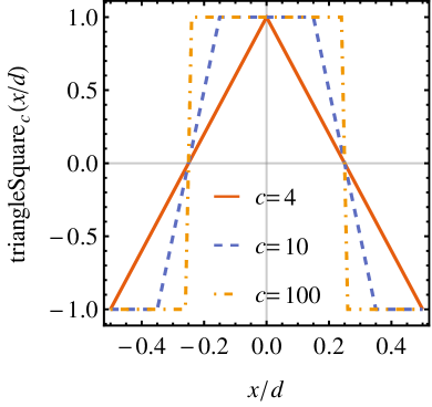
Figure 1: A plot of the $d$-periodic function $\operatorname{triangleSquare}_{c}$ used for defining the potential ${\bf\it A}_{c}^{\text{1D}}$, shown here for three values of $c$. The slope near the points $x=\mp d/4$ is given by $\pm c/d$.

On the other hand in the 2D case we concentrate on the simplest generalization of the 1D cosine-like potential ${\bf\it A}_{\cos}^{\text{1D}}$, the potential

$${\bf\it A}_{\cos}^{\text{2D}}(x,y)=\frac{\beta}{d}(\cos(2\pi y/d),\cos(2\pi x/d))$$ (26)

with the lattice of periodicity being the square superlattice $SL=\operatorname{span}_{\mathbb{Z}}\{{\bf\it t}_{1},{\bf\it t}_{2}\}$, with the primitive vectors ${\bf\it t}_{1}=(d,0)$, ${\bf\it t}_{2}=(0,d)$. Note that we are allowed to choose a potential periodic in any superlattice, whereas in TBG the (moiré) superlattice is fixed by the rotation angle. Thus in principle the periodic strain allows much more freedom in tuning the system. The Fourier components of the 2D cosine potential are

$$\tilde{{\bf\it A}}_{\cos}^{\text{2D}}(m_{1}{\bf\it G}_{1} +m_{2}{\bf\it G}_{2})=$$

$$\frac{\beta}{2d}(\delta_{m_{2},-1}+\delta_{m_{2},1},\delta_{m_{1},-1}+\delta_{m_{1},1})$$ (27)

in the reduced zone scheme, where $m_{1}{\bf\it G}_{1}+m_{2}{\bf\it G}_{2}\in SL_{\text{RZ}}^{*}$ with ${\bf\it G}_{1}=(2\pi/d,0)$ and ${\bf\it G}_{2}=(0,2\pi/d)$.

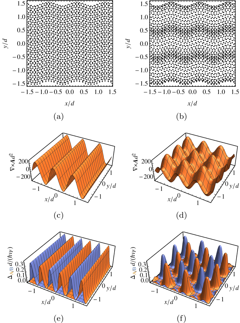
Figure 2: (a,b) Example in-plane displacement fields, defined in (28) and (29), producing the studied pseudo vector potentials ${\bf\it A}_{\cos}^{\text{1D}}$ and ${\bf\it A}_{\cos}^{\text{2D}}$ through (2) with exaggeratedly large amplitude and small period. (c,d) The corresponding pseudomagnetic fields ${\bf\it B}=\nabla\crossproduct{\bf\it A}$ with $\beta=40$ and $\beta=20$, respectively. (e,f) Corresponding typical profiles of the self-consistent superconducting order parameter $\Delta_{A/B}$ ($A$ orange, $B$ blue), which is always peaked at the minima/maxima of $\nabla\crossproduct{\bf\it A}$. The parameters for calculating $\Delta$ are $T=0$, $\lambda/(\hbar v_{\text{F}}d)=-0.01$, and optimal doping $\mu=\mu_{\text{opt}}$ yielding a maximal $\Delta$ ($\mu=0$ produces the same $\Delta$ for such large $\lambda$).

According to (2) the potentials ${\bf\it A}_{\cos}^{\text{1D}}$ and ${\bf\it A}_{\cos}^{\text{2D}}$ can be produced for example by the in-plane displacement fields

$${\bf\it u}_{\cos}^{\text{1D}}(x,y) =\frac{\beta a_{0}}{\beta_{\text{G}}\pi}(0,\sin(2\pi x/d)),$$ (28)

$${\bf\it u}_{\cos}^{\text{2D}}(x,y) =\frac{\beta a_{0}}{\beta_{\text{G}}\pi}(0,\sin(2\pi x/d)+\sin(2\pi y/d)),$$ (29)

respectively. The pseudomagnetic fields ${\bf\it B}=\nabla\crossproduct{\bf\it A}=\partial_{x}A_{y}-\partial_{y}A_{x}$ produced by the 1D and 2D cosine potentials, together with these example displacement fields, are shown in figures 2(a–d). The amplitude $B$ of ${\bf\it B}$, which is an important factor determining the flatness of the bands and the magnitude of the superconducting order parameter $\Delta_{A/B}$, is

$$B_{\cos}^{\text{1D}}=\frac{2\pi\beta}{d^{2}},\quad B_{c}^{\text{1D}}=\frac{c\beta}{d^{2}},\quad B_{\cos}^{\text{2D}}=\frac{4\pi\beta}{d^{2}}$$ (30)

for the potential ${\bf\it A}_{\cos}^{\text{1D}}$, ${\bf\it A}_{c}^{\text{1D}}$, or ${\bf\it A}_{\cos}^{\text{2D}}$, respectively. To give a realistic scale for $\beta$, in the experiment by Jiang et al. Jiang et al. a pseudomagnetic field of $\frac{\hbar}{e}B\approx$100\text{\,}\mathrm{T}$$ was observed for a strain period of $d=$14\text{\,}\mathrm{n}\mathrm{m}$$, which corresponds to $\beta\approx 5$ for the 1D cosine potential. To be better in the flat-band regime, we mostly use a factor of $4$ to $8$ times larger values of $\beta$ in this study.

Corresponding typical profiles of $\Delta_{A/B}$ for the cosine potentials are shown in figures 2(e–f), from where it is clear that $\Delta_{A/B}$ is always peaked at the minima/maxima of the pseudomagnetic field ${\bf\it B}$. For comparison in TBG Peltonen et al. (2018) $\Delta$ is localized around the $AA$ stacking regions and is independent of the sublattice and layer. Note that the sublattice dependence was not present in the work by Kauppila et al. Kauppila et al. (2016) due to sublattice-summation in the self-consistency equation. As we see below, it is approximately the maximum (over position ${\bf\it r}$) of the order parameter that is important in describing the strength of the superconducting state. As for all the studied potentials the maximum of the order parameter is independent of the sublattice, we simply denote $\max\Delta\coloneqq\max\Delta_{A}=\max\Delta_{B}$.

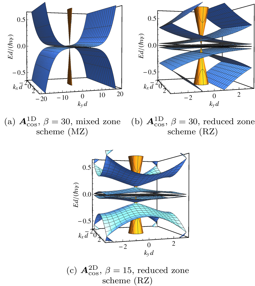
Figure 3: Typical dispersions in the normal state at the valley $\rho=\pm$ with $\mu=0$. (a,b) The 1D cosine potential ${\bf\it A}_{\cos}^{\text{1D}}$ (shown for $\beta=30$) (a) in the mixed zone scheme (MZ) and (b) in the reduced zone scheme (RZ). (c) The 2D cosine potential ${\bf\it A}_{\cos}^{\text{2D}}$ (shown for $\beta=15$) in the reduced zone scheme. The strained dispersions are shown in blue and for comparison the conical unstrained graphene dispersions in orange.

The typical dispersion relations in the normal state are shown in figure 3 together with the conical unstrained graphene dispersions. For an easier comparison the 1D potential ${\bf\it A}_{\cos}^{\text{1D}}$ dispersion is shown both in the mixed zone and reduced zone schemes, while the 2D potential ${\bf\it A}_{\cos}^{\text{2D}}$ dispersion only in the reduced zone scheme (the only possibility in this case). We find similar-looking approximate flat bands as in TBG Peltonen et al. (2018); Julku et al. , with the difference that here the number and the flatness of the flat bands can be controlled by $\beta$ and $c$. Also all the successive bands are touching, while in TBG many models predict the flat bands to be isolated Nam and Koshino (2017); Tarnopolsky et al. (2019); Fang et al. ; Julku et al. .

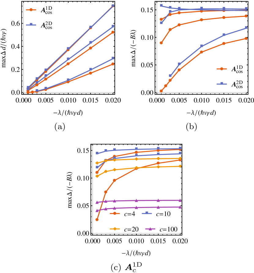
Figure 4: Behavior of the maximum of the superconducting order parameter $\Delta$ as a function of the interaction strength $\lambda$ at optimal doping $\mu=\mu_{\text{opt}}$ and $T=0$. (a) Linearity of $\max\Delta$ in $\lambda$ in the flat-band regime for the cosine potentials. Each potential has three curves corresponding to $\beta=20,30,40$ (1D potential) or $\beta=10,15,20$ (2D potential), from bottom to top. (b,c) The ratio $\max\Delta/(-\lambda B)$ as a function of $\lambda$ for (b) the cosine potentials and (c) ${\bf\it A}_{c}^{\text{1D}}$ with varying $c$, where $B$ is the amplitude of the pseudomagnetic field ${\bf\it B}$. In (b) the curves are the same as in (a) while in (c) each $c$ has two curves corresponding to $\beta=30,40$, from bottom to top. In the flat-band regime the ratio tends approximately to a constant as in (31).

We calculate most of the superconducting state results at optimal doping $\mu=\mu_{\text{opt}}$, which is the energy of the density of states peak as discussed in Sec. III.1, and is thus the doping level with the highest $\Delta$. We start discussing the superconducting state results by calculating $\max\Delta$ as a function of the interaction strength $\lambda$ for the different potentials ${\bf\it A}$, as shown in figures 4(a) for the cosine potentials. The most important conclusion is that for large enough $\lambda$, $\beta$, or $c$, which we call the flat-band regime due to the energy scale of $\Delta$ exceeding the flat-band bandwidth, the dependence is linear in $\lambda$ as we would expect for any flat-band superconductor Heikkilä et al. (2011). On the other hand for small enough $\lambda$, $\beta$, and $c$ the dispersive behavior of the lowest energy bands starts playing a role, which we call the dispersive regime. In the dispersive regime the order parameter is exponentially suppressed and we also start seeing quantum critical points Kopnin and Sonin (2008). We further see how in the flat-band regime the behavior of ${\bf\it A}_{\cos}^{\text{2D}}$ with $\beta$ is similar to that of ${\bf\it A}_{\cos}^{\text{1D}}$ with $2\beta$. Since in this paper we are mostly interested in the flat-band regime, we choose to calculate many of the following results at the fixed interaction strength $\lambda/(\hbar v_{\text{F}}d)=-0.01$, which is clearly in the flat-band regime except for ${\bf\it A}_{\cos}^{\text{2D}}$ with $\beta=10$, which is at the interface of the dispersive and flat-band regimes.

To further confirm that in the flat-band regime $\max\Delta$ is linear both in the interaction strength $\lambda$ and the amplitude $B$ of the pseudomagnetic field ${\bf\it B}$,

$$\max\Delta=-\zeta B\lambda,$$ (31)

we show the ratio $\zeta$ for all the potentials in figures 4(b,c) at $\mu=\mu_{\text{opt}}$ and $T=0$. In the flat-band regime $\zeta$ tends approximately to a constant $\zeta\approx 0.15$, which holds as long as $c\lesssim 20$. For $c\gtrsim 20$ we start seeing deviations from this result, with $\zeta\approx 0.05$ for the extreme case of $c=100$. The small variation in $\zeta$ due to $c$ even in the flat-band regime is most likely due to the fact that the maximum of $\Delta$ is not exactly the correct quantity to calculate, but it gives a very good estimate. We may compare this to the exact-flat-band result Peltonen et al. (2018) with a constant $\Delta^{\text{FB}}$, for which $\Delta^{\text{FB}}=-\frac{1}{(2\pi)^{2}}n\Omega\lambda$ with $\Omega=1/d^{2}$ and $n$ being the number of flat bands. In PSG it is the amplitude $B$ of the pseudomagnetic field ${\bf\it B}$ that effectively determines $n\Omega$, the number of approximate flat bands in the system with the SBZ area of $1/d^{2}$.

III.1 Order parameter profile, dispersion, and density of states

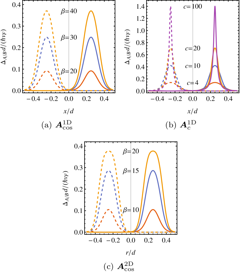
Figure 5: Effect of the amplitude $\beta$ and the slope parameter $c$ on $\Delta_{A/B}$ ($A$ solid, $B$ dashed lines) at $\lambda/(\hbar v_{\text{F}}d)=-0.01$, and optimal doping $\mu=\mu_{\text{opt}}$ ($\mu=0$ produces the same $\Delta$ for such large $\lambda$). (a) Varying $\beta$ of the 1D cosine potential ${\bf\it A}_{\cos}^{\text{1D}}$. (b) Varying the slope parameter $c$ of the 1D potential ${\bf\it A}_{c}^{\text{1D}}$ with $\beta=30$. (c) Varying $\beta$ of the 2D cosine potential ${\bf\it A}_{\cos}^{\text{2D}}$. $\Delta_{A/B}$ is drawn along the line $(x,0)$ [1D potentials] or $r(1,-1)$ [2D potential].

In figure 5 we show a cross section of the self-consistent $\Delta_{A/B}$ [as in figures 2(e,f)] along the line $(x,0)$ [1D potentials] or $r(1,-1)$ [2D potential] for different potentials ${\bf\it A}$, strain strengths $\beta$, and slope parameters $c$. The effect of $\beta$ is to simply linearly increase the amplitude of $\Delta_{A/B}$. On the other hand increasing $c$ not only increases the amplitude of $\Delta_{A/B}$, but makes it also more localized. We also see that for the 2D potential ${\bf\it A}_{\cos}^{\text{2D}}$, $\Delta_{A/B}$ with the strain strength $\beta$ along the diagonal behaves similarly as $\Delta_{A/B}$ in the $x$ direction for the 1D potential ${\bf\it A}_{\cos}^{\text{1D}}$ with $2\beta$.

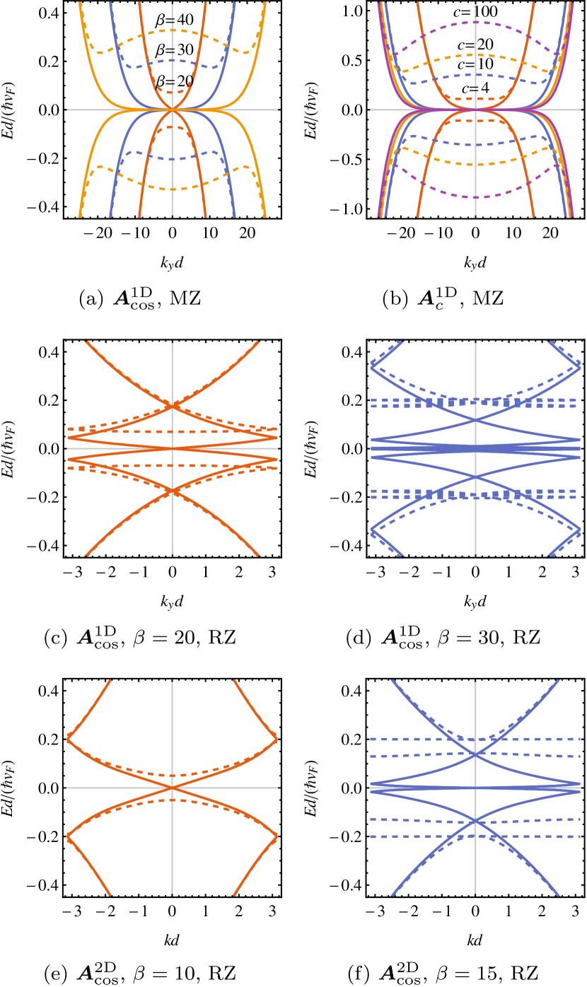
Figure 6: Effect of the strain strength $\beta$ and the slope parameter $c$ on the dispersion (normal state: solid, superconducting state: dashed lines) for the different potentials at $\mu=0$. In the superconducting state $T=0$ and $\lambda/(\hbar v_{\text{F}}d)=-0.01$. (a,b) Dispersions in the mixed zone scheme (MZ) along the line $(k_{y},0)$ for (a) ${\bf\it A}_{\cos}^{\text{1D}}$ with various $\beta$ and for (b) ${\bf\it A}_{c}^{\text{1D}}$ with various $c$ and fixed $\beta=30$. (c,d) Corresponding dispersions in the reduced zone scheme (RZ) along the line $(0,k_{y})$ for ${\bf\it A}_{\cos}^{\text{1D}}$ with $\beta=20$ and $30$, respectively. (e,f) Dispersions for ${\bf\it A}_{\cos}^{\text{2D}}$ along the diagonal line $k(1,1)$ in the reduced zone scheme for $\beta=10$ and $15$, respectively.

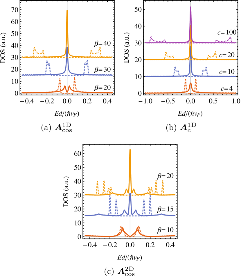
Figure 7: Effect of the strain strength $\beta$ and the slope parameter $c$ on the density of states (DOS) at $\mu=0$, $T=0$, and $\lambda/(\hbar v_{\text{F}}d)=-0.01$ (normal state: solid, superconducting state: dashed lines) for (a) ${\bf\it A}_{\cos}^{\text{1D}}$, (b) ${\bf\it A}_{c}^{\text{1D}}$, and (c) ${\bf\it A}_{\cos}^{\text{2D}}$. For clarity the successive curves in the DOS plots are shifted vertically by $15$ in (a,c) and by $7$ in (b). Each curve is normalized such that the shown area integrates to unity.

These effects we can further see in the dispersions and densities of states in figures 6 and 7, respectively, which are plotted at $\mu=0$ for clarity. In figure 6 we show the cross section of the dispersions in figure. 3 along the line $(0,k_{y})$ [1D potentials] or $k(1,1)$ [2D potential], both in the normal and superconducting states, and in the different schemes to allow for easier comparison between the 1D and 2D potentials. In figure 7 we show the corresponding densities of states (DOS). We clearly see in the normal state how increasing $\beta$ and $c$ both suppress the group velocity, thus increasing flatness of the bands. The density of states becomes correspondingly more and more peaked at zero energy. The superconducting energy gap also increases both with increasing $\beta$ and $c$, and the peculiar double-peak structure in the superconducting DOS is also better revealed for higher $\beta$ or $c$. In the 2D case it is notable how increasing $\beta$ generates multiple peaks in the normal state DOS, and thus also in the superconducting state DOS, in a way that separates it from the 1D potentials.

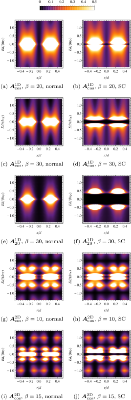
Figure 8: Local density of states (LDOS) at $\mu=0$ and $T=0$ along the line $(x,0)$ [1D potentials] or $r(1,-1)$ [2D potential] both in the (a,c,e,g,i) normal and (b,d,f,h,j) superconducting (SC) states. In the superconducting state $\lambda/(\hbar v_{\text{F}}d)=-0.01$. In each plot the states on the positive (negative) $x$ or $r$ side is coming from the sublattice $A$ ($B$). Each plot is normalized such that the total visible area integrates to unity.

To determine more properties that could be measured e.g. by STM Xie et al. (2019); Jiang et al. , we show in figure 8 the local densities of states (LDOS) along the line $(x,0)$ [1D potentials] or $r(1,-1)$ [2D potential], which further illustrate the results discussed so far. In the normal state the overall energy dependence shows the clear peak at zero energy for the 1D potentials, as well as the multiple-peak structure for the 2D potential. In the superconducting state the energy dependence also shows the superconducting gap, as already seen in the total DOS in figure 7. The position dependence gives us more information about the underlying strain field. They clearly show the high density of low-energy states near the points $x=\pm d/4$ (1D potentials) or $r=\pm d/4$ (2D potential), that is, points where ${\bf\it B}$ has extrema. Furthermore the states on the positive (negative) $x$ or $r$ side are those coming from the sublattice $A$ ($B$), which, by comparison to Fig. 2(c–d), means that the $A$ ($B$) sublattice states are localized at the minima (maxima) of ${\bf\it B}$. This kind of localization and sublattice polarization was also experimentally observed by Jiang et al. Jiang et al. . Since the low-energy states are the ones contributing to superconductivity, their localization explains the similar localization of the order parameter $\Delta_{A/B}$, as seen in figures 2(e,f).

In the normal state LDOS we further see the localization pattern splitting at higher energies for the 1D potentials. This is contrasted with the 2D potential, where the higher-energy peaks are separated not only in position but also in energy. Furthermore in the superconducting state LDOS we see the same behavior in the energy gaps as in the total DOS: increasing $\beta$ or $c$ leads to an increasing gap size, with the localization pattern staying the same. Again the 2D potential behaves slightly differently: the gap is largest at $r=\pm d/4$, while for the 1D potentials the gap at $x=\pm d/4$ is smallest.

III.2 Critical doping level and temperature

We can in principle calculate the critical doping level $\mu_{\text{c}}$ and the critical temperature $T_{\text{c}}$ by solving the self-consistency equation (19) for various $\mu$ and $T$ and by solving for the point where $\Delta$ vanishes. But since the fixed-point iteration scheme converges slowly when $\Delta$ is small, we calculate $\mu_{$50\text{\,}\mathrm{\char 37\relax}$}$ [$T_{$50\text{\,}\mathrm{\char 37\relax}$}$] instead, corresponding to the chemical potential [temperature] at which $\max\Delta$ has decreased to $\max\Delta(\mu=0)/2$ [$\max\Delta(T=0)/2$].

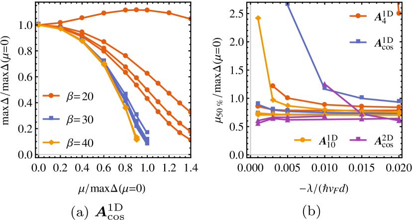
Figure 9: Solving the “critical” chemical potential $\mu_{$50\text{\,}\mathrm{\char 37\relax}$}$ at $T=0$, where $\mu_{$50\text{\,}\mathrm{\char 37\relax}$}$ is the chemical potential where $\max\Delta$ has dropped to $\max\Delta(\mu=0)/2$. (a) Normalized order parameter maximum $\max\Delta/\max\Delta(\mu=0)$ as a function of the normalized chemical potential $\mu/\max\Delta(\mu=0)$ for ${\bf\it A}_{\cos}^{\text{1D}}$ showing how doping away from the flat band, located at the DOS peak (which is at the zero energy in the flat-band regime and at a nonzero energy in the dispersive regime), kills superconductivity. The behavior is the same for $-\mu$. The four curves for each $\beta$ are those for $-\lambda/(\hbar v_{\text{F}}d)=0.005,0.01,0.015,0.02$ (from top to bottom). (b) The ratio $\mu_{$50\text{\,}\mathrm{\char 37\relax}$}/\max\Delta(\mu=0)$ as a function of $\lambda$ for different potentials ${\bf\it A}$. Each 1D potential has three curves corresponding to $\beta=20,30,40$ (from top to bottom). In the flat-band regime the ratio tends approximately to a constant as in (32).

We show in figure 9(a) the $\mu$-dependence of $\Delta$ at $T=0$ in the case of ${\bf\it A}_{\cos}^{\text{1D}}$, from where $\mu_{$50\text{\,}\mathrm{\char 37\relax}$}$ is determined. We see how doping away from the flat band, which in the flat-band regime is located at zero energy, kills superconductivity. In this case $\mu_{$50\text{\,}\mathrm{\char 37\relax}$}$ approaches $\sim 0.7\max\Delta(\mu=0)$ in the flat-band limit. In the flat-band regime the results fit very well the relation $\max\Delta(\mu)=\sqrt{(\max\Delta(\mu=0))^{2}-(\mu/b)^{2}}$ with $b$ as the fitting parameter, as compared to the result Heikkilä and Volovik (2016) $\Delta^{\text{FB}}(\mu)=\sqrt{\Delta^{\text{FB}}(\mu=0)^{2}-\mu^{2}}$ for exactly flat bands and homogeneous $\Delta^{\text{FB}}$. On the other hand in the dispersive regime $\Delta$ is not maximized at zero chemical potential, but around $\mu\approx 0.9\max\Delta(\mu=0)\approx\frac{0.9}{1.1}\max\Delta(\mu=\mu_{\text{opt}})\approx 0.02\hbar v_{\text{F}}/d$ instead, which corresponds to the DOS peak position shown in figure 7(a). This is exactly the same behavior as seen in TBG Peltonen et al. (2018); Wu et al. (2018): in the flat-band regime the energy scale of $\Delta$ exceeds the DOS peak separation (the “bandwidth”) and the smeared DOS is centered at zero energy, while in the dispersive regime $\Delta$ can “see” the double-peaked DOS because of the small energy scale of $\Delta$. In TBG this might explain Peltonen et al. (2018); Wu et al. (2018) why superconductivity is observed at a nonzero doping level Cao et al. (2018), and the same might happen also in PSG if the interaction strength $\lambda$ is small enough. But note that in PSG we can in principle tune ${\bf\it A}$ (its functional dependence, $\beta$, $c$, and $d$) to move the interface between the flat-band and dispersive regimes so that superconductivity would be observed at zero doping.

To further verify that $\mu_{$50\text{\,}\mathrm{\char 37\relax}$}$ is linear in $\max\Delta(\mu=0)$ in the flat-band regime,

$$\mu_{$50\text{\,}\mathrm{\char 37\relax}$}=\eta\max\Delta(\mu=0),$$ (32)

we show in figure 9(b) the ratio $\eta$ at $T=0$ for a selection of potentials. In the flat-band regime the ratio tends approximately to a constant $\eta\approx 0.7$ as long as $c\lesssim 10$. For $c\gtrsim 10$ we start seeing slight deviations from this, with $\eta\approx 0.6$ and $0.5$ for $c=20$ and $100$, respectively. The critical chemical potential $\mu_{\text{c}}$ is slightly larger, approximately $\mu_{\text{c}}\approx\max\Delta(\mu=0)$ for ${\bf\it A}_{\cos}^{\text{1D}}$ in the flat-band regime according to figure 9(a). This coincides with the case of perfectly flat bands and a constant $\Delta^{\text{FB}}$ for which [Peltonen et al., 2018, Supplemental Material] $\mu_{\text{c}}^{\text{FB}}=\Delta^{\text{FB}}(\mu=0)$.

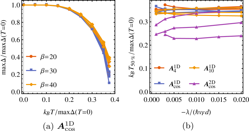
Figure 10: Solving the “critical” temperature $T_{$50\text{\,}\mathrm{\char 37\relax}$}$ at optimal doping $\mu=\mu_{\text{opt}}$, where $T_{$50\text{\,}\mathrm{\char 37\relax}$}$ is the temperature where $\max\Delta$ has dropped to $\max\Delta(T=0)/2$. (a) Normalized order parameter maximum $\max\Delta/\max\Delta(T=0)$ as a function of the normalized temperature $k_{\text{B}}T/\max\Delta(T=0)$ for ${\bf\it A}_{\cos}^{\text{1D}}$. Each $\beta$ has four curves corresponding to $-\lambda/(\hbar v_{\text{F}}d)=0.005,0.01,0.015,0.02$. (b) The ratio $k_{\text{B}}T_{$50\text{\,}\mathrm{\char 37\relax}$}/\max\Delta(T=0)$ as a function of $\lambda$ for different potentials ${\bf\it A}$. Each ${\bf\it A}$ has three curves corresponding to $\beta=20,30,40$ (1D potentials) or $\beta=10,15,20$ (2D potential), with the outliers being those for the smallest $\beta$. In the flat-band regime the ratio tends approximately to a constant as in (33).

In figure 10 we show the corresponding plots for determining $T_{$50\text{\,}\mathrm{\char 37\relax}$}$ at $\mu=\mu_{\text{opt}}$. Again the ratio $\xi$ in

$$k_{\text{B}}T_{$50\text{\,}\mathrm{\char 37\relax}$}=\xi\max\Delta(T=0),$$ (33)

tends approximately to a constant $\xi\approx 0.35$ in the flat-band regime as long as $c\lesssim 10$. For $c\gtrsim 10$ we start seeing deviations from this, with $\xi\approx 0.3$ for $c=20$ and $\xi\approx 0.25$ for $c=100$. The critical temperature $T_{\text{c}}$ is slightly larger, approximately $k_{\text{B}}T_{\text{c}}\approx 0.4\max\Delta(T=0)$ for ${\bf\it A}_{\cos}^{\text{1D}}$ in the flat-band regime according to figure 10(a). For comparison, in the case of perfectly flat bands and a constant $\Delta^{\text{FB}}$ we have the result Heikkilä et al. (2011) $k_{\text{B}}T_{\text{c}}^{\text{FB}}=\frac{1}{2}\Delta^{\text{FB}}(T=0)$ and in TBG Peltonen et al. (2018) within the same interaction model $k_{\text{B}}T_{\text{c}}\approx 0.25\max\Delta(T=0)$.

III.3 Superfluid weight and Berezinskii–Kosterlitz–Thouless transition temperature

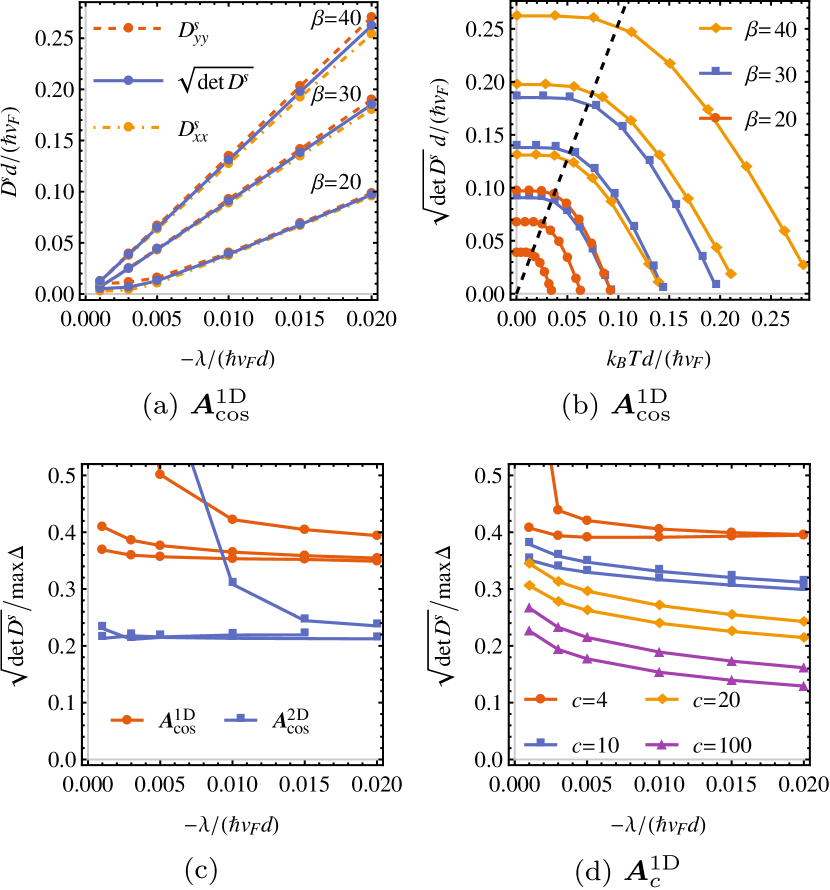
Figure 11: Behavior of the superfluid weight $D^{\text{s}}$ at optimal doping $\mu=\mu_{\text{opt}}$ and (a,c,d) $T=0$. (a) $D^{\text{s}}$ as a function of $\lambda$ for ${\bf\it A}_{\cos}^{\text{1D}}$ showing linearity in the flat-band regime. The superfluid weight for the 1D potentials is slightly anisotropic, $D^{\text{s}}_{xx}\neq D^{\text{s}}_{yy}$, for large $\beta$ and $\lambda$. For the 2D potential ${\bf\it A}_{\cos}^{\text{2D}}$ (not shown) the superfluid weight is isotropic, $D^{\text{s}}_{xx}=D^{\text{s}}_{yy}$. The off-diagonal components $D^{\text{s}}_{xy}=0=D^{\text{s}}_{xy}$ are zero for all the studied potentials. The (an)isotropy is consistent with the symmetries of the studied potentials. (b) $\sqrt{\det D^{\text{s}}}$ as a function of temperature $T$ for ${\bf\it A}_{\cos}^{\text{1D}}$. Each $\beta$ has three curves corresponding to $-\lambda/(\hbar v_{\text{F}}d)=0.01,0.015,0.02$, from bottom to top. Also the dashed line $\sqrt{\det D^{\text{s}}}=8k_{\text{B}}T/\pi$ is shown, from intersections of which $T_{\text{BKT}}$ is determined through (21). (c,d) The ratio $\sqrt{\det D^{\text{s}}}/\max\Delta$ as a function of the interaction strength $\lambda$ for (c) the cosine potentials and (d) ${\bf\it A}_{c}^{\text{1D}}$ with varying $c$. In (c) each ${\bf\it A}$ has three curves corresponding to (from top to bottom) $\beta=20,30,40$ (1D potentials) or $\beta=10,15,20$ (2D potential), while in (d) each $c$ has two curves corresponding to (from top to bottom) $\beta=30,40$. In the flat-band regime the ratio is approximately a constant depending slightly on the potential, as in (34).

To determine the true superconducting transition temperature we calculate the superfluid weight $D^{\text{s}}$ and the Berezinskii–Kosterlitz–Thouless transition temperature $T_{\text{BKT}}$ from (20) and (21). In figure 11(a) we show the total superfluid weight $\sqrt{\det D^{\text{s}}}$, together with the different components $D^{\text{s}}_{\mu\nu}$, as a function of the interaction strength $\lambda$ for ${\bf\it A}_{\cos}^{\text{1D}}$. The behavior is very similar to that of $\max\Delta$ in figure 4(a): it is linear in the flat-band regime and also increases linearly with increasing $\beta$. To further verify that $\sqrt{\det D^{\text{s}}}$ is linear in $\max\Delta$,

$$\sqrt{\det D^{\text{s}}}=\chi\max\Delta,$$ (34)

we show the ratio $\chi$ in figure 11(c,d) at $\mu=\mu_{\text{opt}}$ and $T=0$. In the flat-band regime the ratio tends approximately to a constant $\chi\approx 0.15\dots 0.4$, which has more variation than $\eta$ and $\xi$ for $\mu_{$50\text{\,}\mathrm{\char 37\relax}$}$ and $T_{$50\text{\,}\mathrm{\char 37\relax}$}$ in the flat-band regime. For comparison, in TBG we found Julku et al. within the same interaction model that $\chi\approx 0.35$ in the flat-band regime.

We may again compare (34) to the case of exactly flat bands and a constant $\Delta^{\text{FB}}$. But since the superfluid weight depends heavily on the Hamiltonian itself and not only its eigenvalues, we need to specify which flat-band model to use. We take the “graphene flat-band limit”, that is, graphene with $v_{\text{F}}\rightarrow 0$. In this case Kopnin and Sonin (2010); Liang et al. (2017) $D^{\text{s}}_{\text{FB}}=\frac{2}{\pi}\Delta^{\text{FB}}$ at $\mu=0\approx\mu_{\text{opt}}$ and $T=0$, which in fact holds for any $v_{\text{F}}$.

What is intriguing in figure 11(a) is that for the studied 1D potentials the superfluid weight is almost isotropic although the potentials are highly anisotropic. There is, however, a slight anisotropy, $D^{\text{s}}_{xx}\neq D^{\text{s}}_{yy}$ and $D^{\text{s}}_{xy}=0=D^{\text{s}}_{yx}$, visible for large $\beta$ and $\lambda$. On the other hand the 2D potential produces an isotropic superfluid weight, $D^{\text{s}}_{xx}=D^{\text{s}}_{yy}$ and $D^{\text{s}}_{xy}=0=D^{\text{s}}_{yx}$. This (an)isotropy is consistent with the symmetries of the studied potentials. For comparison in TBG it was found Julku et al. that local interaction always produces an isotropic superfluid weight, while the more complicated resonating valence bond (RVB) interaction was able to produce anisotropy through spontaneous symmetry breaking. The anisotropy could serve as one experimental signature for superconductivity described by the presented model, and it could be measured by radio frequency impedance spectroscopy Chiodi et al. (2011) in a Hall-like four-probe setup Julku et al. .

Although in this work we do not separate the superfluid weight into the conventional and geometric contributions Liang et al. (2017), from general knowledge Liang et al. (2017) and calculations in TBG Julku et al. ; Hu et al. we expect the geometric contribution to dominate in the flat-band regime.

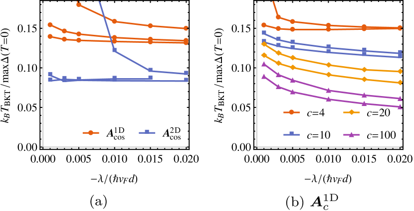
Figure 12: Behavior of the Berezinskii–Kosterlitz–Thouless transition temperature $T_{\text{BKT}}$ at optimal doping $\mu=\mu_{\text{opt}}$. The ratio $k_{\text{B}}T_{\text{BKT}}/\max\Delta(T=0)$ for (a) the cosine potentials and (b) ${\bf\it A}_{c}^{\text{1D}}$ with varying $c$. In (a) both potentials have three curves corresponding to $\beta=20,30,40$ (1D potential) or $\beta=10,15,20$ (2D potential), from top to bottom in the flat-band regime, while in (b) each $c$ has two curves corresponding to $\beta=30,40$, from top to bottom. In the flat-band regime the ratio tends approximately to a constant depending slightly on the potential, as in (35). Due to slow convergence the approximation $D^{\text{s}}(T_{\text{BKT}})\approx D^{\text{s}}(0)$ is used for the ${\bf\it A}_{\cos}^{\text{2D}}$ potential.

In figure 11(b) we further show $\sqrt{\det D^{\text{s}}}$ as a function of temperature $T$ for ${\bf\it A}_{\cos}^{\text{1D}}$, from where $T_{\text{BKT}}$ is determined through (21) by solving for the intersection point with the line $\sqrt{\det D^{\text{s}}}=8k_{\text{B}}T/\pi$. We immediately see that in the flat-band regime $D^{\text{s}}(T_{\text{BKT}})\approx D^{\text{s}}(0)$ is a rather good approximation so that the self-consistency in (21) is not essential. This is very different from TBG Julku et al. , where the temperature dependence is essential due to $T_{\text{BKT}}$ being closer to $T_{\text{c}}$. We nevertheless need to solve the full self-consistent equation for all the potentials, as the relative magnitude of $T_{\text{c}}$ and $T_{\text{BKT}}$ is not known beforehand.

The resulting ratio $k_{\text{B}}T_{\text{BKT}}/\max\Delta(T=0)$ is shown in figure 12 for the different potentials at $\mu=\mu_{\text{opt}}$, further confirming that $D^{\text{s}}(T_{\text{BKT}})\approx D^{\text{s}}(0)$: apart from the different scale, the $T_{\text{BKT}}$ plots in figure 12 are very similar to the $D^{\text{s}}$ plots in figures 11(c,d). Furthermore in the linear relation

$$k_{\text{B}}T_{\text{BKT}}=\kappa\max\Delta(T=0),$$ (35)

the ratio $\kappa$ tends approximately to a constant $\kappa\approx 0.05\dots 0.15$ in the flat-band regime. Again in (35) we see similarity to the “graphene flat-band limit” result with a homogeneous $\Delta^{\text{FB}}$, for which $k_{\text{B}}T_{\text{BKT}}^{\text{FB}}=\frac{\pi}{8}D^{\text{s}}_{\text{FB}}(T_{\text{BKT}}^{\text{FB}})\approx\frac{1}{4}\Delta^{\text{FB}}(T=0)$ at $\mu=0\approx\mu_{\text{opt}}$ if we furthermore assume $D^{\text{s}}_{\text{FB}}(T_{\text{BKT}}^{\text{FB}})\approx D^{\text{s}}_{\text{FB}}(0)$.

Combining (34) and (35) we get in the flat-band regime at $\mu=\mu_{\text{opt}}$ the ratio $T_{\text{BKT}}/T_{$50\text{\,}\mathrm{\char 37\relax}$}=\kappa/\xi\approx 0.2\dots 0.4$ depending on the potential. For ${\bf\it A}_{\cos}^{\text{1D}}$ this yields $T_{\text{BKT}}/T_{$50\text{\,}\mathrm{\char 37\relax}$}\approx 0.4$, and within the same accuracy $T_{\text{BKT}}/T_{\text{c}}\approx 0.4$. For comparison in TBG we found within the same interaction model in the flat-band regime $k_{\text{B}}T_{\text{BKT}}\approx 0.16\dots 0.2\max\Delta(T=0)$ Julku et al. (depending slightly on $\lambda$), $k_{\text{B}}T_{\text{c}}\approx 0.25\max\Delta(T=0)$ Peltonen et al. (2018), and thus $T_{\text{BKT}}/T_{\text{c}}\approx 0.6\dots 0.8$.

By combining (31) and (35) we get $k_{\text{B}}T_{\text{BKT}}=-\kappa\zeta B\lambda$ at $\mu=\mu_{\text{opt}}$. Let us calculate an estimate of $T_{\text{BKT}}$ by using $\lambda=-$1\text{\,}\mathrm{e}\mathrm{V}$a^{2}\approx-$6\text{\,}\mathrm{e}\mathrm{V}\mathrm{\SIUnitSymbolAngstrom}^{2}$$, which roughly corresponds Peltonen et al. (2018); Julku et al. to $T_{\text{BKT}}\approx$1\text{\,}\mathrm{K}$$ measured in TBG Cao et al. (2018). Here $a=\sqrt{3}a_{0}\approx$2.46\text{\,}\mathrm{\SIUnitSymbolAngstrom}$$ is the graphene lattice constant. For ${\bf\it A}_{\cos}^{\text{1D}}$ we have $B=2\pi\beta/d^{2}$ and in the flat-band regime $\kappa=0.15$ and $\zeta=0.15$, yielding a similar $T_{\text{BKT}}\approx$1\text{\,}\mathrm{K}$$ if we apply strain for example such that $\beta=40$ and $d=$60\text{\,}\mathrm{n}\mathrm{m}$$ [then $\lambda/(\hbar v_{\text{F}}d)\approx-0.002$ if using $v_{\text{F}}=$1\text{\times}{10}^{6}\text{\,}\mathrm{m}\mathrm{/}\mathrm{s}$$, which is in the flat-band regime according to figures 4(b) and 12(a)]. In the case of the in-plane displacement field ${\bf\it u}_{\cos}^{\text{1D}}$ (28) this corresponds to the displacement amplitude $\beta a_{0}/(\beta_{\text{G}}\pi)\approx$1\text{\,}\mathrm{n}\mathrm{m}$$ if $\beta_{\text{G}}=2$. Since in this case the elasticity theory assumes $\beta/\beta_{\text{G}}\ll d/a_{0}$ and $d/a_{0}\gg 1$ sup , we are very well in the validity regime. On the other hand, if we are able to decrease the strain period to $d=$10\text{\,}\mathrm{n}\mathrm{m}$$ [then $\lambda/(\hbar v_{\text{F}}d)=-0.009$], we get to a high-temperature superconductor value of $T_{\text{BKT}}\approx$40\text{\,}\mathrm{K}$$, which is still in the validity regime. Note the optimization problem in increasing $T_{\text{BKT}}$: decreasing $d$ directly enhances $T_{\text{BKT}}$ but at the same time it makes the validity limit for $\beta$ tighter, while at the same time we should have as large $\beta$ as possible. But this might only be a limiting factor in our linear elasticity theory, while a more complete microscopic theory could, perhaps, yield a result that increasing $\beta$ or decreasing $d$ always increases $T_{\text{BKT}}$.

The experiments of Jiang et al. Jiang et al. with $\frac{\hbar}{e}B\approx$100\text{\,}\mathrm{T}$$ and $d=$14\text{\,}\mathrm{n}\mathrm{m}$$ can be described by the 1D cosine potential with $\beta\approx 5$. When $\lambda=$-6\text{\,}\mathrm{e}\mathrm{V}\mathrm{\SIUnitSymbolAngstrom}^{2}$$, $\lambda/(\hbar v_{\text{F}}d)\approx-0.007$ is not in the flat-band regime. Hence $T_{\text{BKT}}$ cannot be obtained from the simple estimate used above, and is likely much lower than $1\text{\,}\mathrm{K}$. Increasing the strain amplitude by a factor of $4$, so that $\beta=20$, would yield $\zeta=0.05$, $\kappa=0.17$, and thus $T_{\text{BKT}}\approx 0.007\hbar v_{\text{F}}/(dk_{\text{B}})\approx$4\text{\,}\mathrm{K}$$. Further decreasing the period to $d=$8\text{\,}\mathrm{n}\mathrm{m}$$, a period which was already observed by Jiang et al., would yield already $\lambda/(\hbar v_{\text{F}}d)\approx-0.01$ and thus $T_{\text{BKT}}\approx$11\text{\,}\mathrm{K}$$.

IV Conclusions

We have studied both the normal and superconducting $s$-wave state properties of periodically strained graphene (PSG) in the continuum low-energy model. We have shown that periodic strain might be a mechanism that allows increasing the critical temperature $T_{\text{c}}$ higher than a few kelvin, observed in doped graphene and in twisted bilayer graphene (TBG), or possibly even to tens of kelvins. Especially we have generalized the results of Kauppila et al. Kauppila et al. (2016), where the authors studied the same problem in the case of a 1D cosine-like pseudo vector potential ${\bf\it A}$, to potentials with arbitrary shape and dimension. We furthermore calculated the superfluid weight and the Berezinskii–Kosterlitz–Thouless transition temperature $T_{\text{BKT}}$ to determine the true transition temperature observed in experiments. In the normal state we observed flat bands in the spectrum and localization of low-energy states near the extremum points of the effective magnetic field ${\bf\it B}=\nabla\crossproduct{\bf\it A}$.

We modelled the superconducting state by the Bogoliubov–de Gennes mean-field theory assuming a local interaction between the Cooper pair leading to $s$-wave pairing. Because of the inhomogeneous strain field we observed a highly inhomogeneous order parameter $\Delta_{A/B}$ that is localized near the extremum points of ${\bf\it B}$, similarly to the localization of the low-energy states. We also noticed how the superconducting $T_{\text{c}}$ or $T_{\text{BKT}}$ can be linearly increased by increasing the strain strength $\beta$, decreasing the period $d$, or by increasing the slope (near the extremum points of ${\bf\it B}$) of the corresponding pseudo vector potential ${\bf\it A}$. On the other hand increasing the slope makes the order parameter also more localized.

While between the 1D potentials we observed only quantitative differences in the results, for the 2D cosine potential we saw also some qualitative differences when compared to the 1D potentials. The main differences are the localization pattern of $\Delta_{A/B}$, and the more peaked structure of the (local) density of states both in the normal and superconducting states. In the 2D case we studied only the cosine potential, but on the other hand the qualitative similarity in the results between the different 1D potentials gives us certainty that changing the shape of the potential would not change the qualitative results in the 2D case neither. However, it should be noted that it is the shape of ${\bf\it B}$ that matters and not that of the potential ${\bf\it A}$ itself, and thus even a 2D potential can produce results that are effectively those of a 1D potential.

We chose all our potentials to be periodic in a square (super)lattice, but note that any other lattice could be chosen as well, with different shapes and different periodicities in the two directions. Properties of this lattice are then directly seen in the dispersion, as well as in the localization of ${\bf\it B}$ and $\Delta_{A/B}$. We also observed the symmetry $\Delta_{B}({\bf\it r})=\Delta_{A}(-{\bf\it r})$ of the order parameter for all the chosen potentials. This is due to the inversion symmetry ${\bf\it A}({\bf\it r})={\bf\it A}(-{\bf\it r})$ present in all of them. The relative magnitude between $\Delta_{A}$ and $\Delta_{B}$ can then be tuned by breaking this symmetry, e.g. by using a sawtooth-wave potential.

We also observed some very peculiar structures in the (local) density of states, which could serve as an experimental fingerprint of the physics described by this model. We furthermore found that in the flat-band regime the superconducting order parameter maximum $\max\Delta$ at $\mu=\mu_{\text{opt}}$ and $T=0$, the “critical” chemical potential $\mu_{$50\text{\,}\mathrm{\char 37\relax}$}$ at $T=0$, the “critical” temperature $T_{$50\text{\,}\mathrm{\char 37\relax}$}$ at $\mu=\mu_{\text{opt}}$, the superfluid weight $\sqrt{\det D^{\text{s}}}$ at $\mu=\mu_{\text{opt}}$ and $T=0$, and the BKT transition temperature $T_{\text{BKT}}$ at $\mu=\mu_{\text{opt}}$ are all approximately linear in the interaction strength $\lambda$. The linear relations, instead of exponential ones in usual bulk superconductors, suggest that high-temperature superconductivity might be possible in PSG.

As is known from TBG, also other phases like correlated insulators might be present due to the flat bands. These are obviously excluded from the present study, but as we showed in a previous study Peltonen et al. (2018), the superconductivity-only model gives a plausible explanation for the observed superconducting states in TBG. This view of competing phases is supported by recent experiments where superconductivity could be seen without the correlated insulating phases Stepanov et al. ; Saito et al. . Thus we expect our similar model to work also in PSG when concentrating only on superconductivity. If the competing phase (if any) is magnetic, we know from a recent study Ojajärvi et al. (2018) that in a pure flat-band system superconductivity is favored over magnetism whenever (in the weak coupling regime) the effective attractive electron–electron interaction strength $\hat{\lambda}\hbar\omega_{\text{c}}=[g^{2}/(\hbar\omega_{\text{c}})](\Omega_{\text{FB}}/\Omega_{\text{BZ}})$ is stronger than the repulsive one $u=U\Omega_{\text{FB}}/\Omega_{\text{BZ}}$. Here $g$ is the electron–phonon coupling constant, $U$ is the repulsive Hubbard coupling constant, $\hbar\omega_{\text{c}}$ is the characteristic phonon energy (in this case the Einstein energy $\hbar\omega_{E}$), and $\Omega_{\text{FB}}/\Omega_{\text{BZ}}$ is the ratio of the flat-band area to the Brillouin zone area.

An interesting future prospect would be to study the other phases which, by the analogue of TBG, are highly probable. Secondly the combination of moiré Peltonen et al. (2018) and strain [this work] physics would perhaps advance the understanding of superconductivity in TBG, where intrinsic periodic strain is inevitable. From the experimental point of view the challenge is to manufacture periodically strained graphene samples with large amplitudes and small periods and to perform low-temperature conductivity measurements in this (electrically doped) system to reveal the possible superconducting and/or correlated insulator states. The periodic strain and flat bands observed by Jiang et al. Jiang et al. are already an intriguing starting point, but according to our calculations a $T_{\text{BKT}}$ of the order of $4\text{\,}\mathrm{K}$ would need a strain amplitude $4$ times larger than in the experiment. On the other hand, further decreasing the period to $8\text{\,}\mathrm{n}\mathrm{m}$ would yield already $T_{\text{BKT}}\approx$11\text{\,}\mathrm{K}$$.