Manifold spirals in barred galaxies with multiple pattern speeds

Abstract

In the manifold theory of spiral structure in barred galaxies, the usual assumption is that the spirals rotate with the same pattern speed as the bar. Here we generalize the manifold theory under the assumption that the spirals rotate with different pattern speed than the bar. More generally, we consider the case when one or more modes, represented by the potentials $V_{2}$, $V_{3}$, $\ldots$, co-exist in the galactic disc in addition to the bar’s mode $V_{bar}$, but rotate with pattern speeds $\Omega_{2}$, $\Omega_{3}$, $\ldots$ incommensurable between themselves and with $\Omega_{bar}$. Through a perturbative treatment (assuming that $V_{2},V_{3}...$ are small with respect to $V_{bar}$) we then show that the unstable Lagrangian points $L_{1}$, $L_{2}$ of the pure bar model $(V_{bar},\Omega_{bar})$ are ‘continued’ in the full model as periodic orbits, when we have one extra pattern speed different from $\Omega_{bar}$, or as epicyclic ‘Lissajous-like’ unstable orbits, when we have more than one extra pattern speeds. We denote by $GL_{1}$ and $GL_{2}$ the continued orbits around the points $L_{1}$, $L_{2}$, and we show that the orbits $GL_{1}$ and $GL_{2}$ are simply unstable. As a result, these orbits admit invariant manifolds which can be regarded as the generalization of the manifolds of the $L_{1}$,$L_{2}$ points in the single pattern speed case. As an example we compute the generalized orbits $GL_{1}$, $GL_{2}$ and their manifolds in a Milky-way like model with bar and spiral pattern speeds assumed different. We find that the manifolds produce a time-varying morphology consisting of segments of spirals or ‘pseudorings’. These structures are repeated after a period equal to half the relative period of the imposed spirals with respect to the bar. Along one period, the manifold-induced time-varying structures are found to continuously support at least some part of the imposed spirals, except at short intervals around those times at which the relative phase of the imposed spirals with respect to the bar becomes equal to $\pm\pi/2$. A connection of these effects to the phenomenon of recurrent spirals is discussed.

I Introduction

The manifold theory of spiral structure in barred galaxies (Romero-Gomez et al. (2006); Voglis et al. (2006)) predicts bi-symmetric spirals emanating from the end of galactic bars as a result of the outflow of matter connected with the unstable dynamics around the bar’s Lagrangian points $L_{1}$ and $L_{2}$ (see also Danby (1965)). The manifold theory has been expressed in two versions, namely the ‘flux-tube’ version (Romero-Gomez et al. (2006); Romero-Gomez et al. (2007); Athanassoula et al. (2009a); Athanassoula et al. (2009b); Athanassoula (2012)) and the ‘apocentric manifold’ version (Voglis et al. (2006); Tsoutsis et al. (2008); Tsoutsis et al. (2009); Harsoula et al. (2016)). In both versions, the orbits of stars along the manifolds are chaotic, thus the manifolds provide a skeleton of orbits supporting ‘chaotic spirals’ (Patsis (2006)). Furthermore, the theory predicts that the orbital flow takes place in a direction preferentially along the spirals. This is in contrast to standard density wave theory (Lin & Shu (1964); see Binney & Tremaine (2008)), which predicts a regular orbital flow forming ‘precessing ellipses’ (Kalnajs (1973)) which intersect the spirals. This difference has been proposed as an observational criterion to distinguish chaotic (manifold) from regular (density wave) spirals (Patsis (2006)).

Among a number of objections to manifold theory (see introduction in Efthymiopoulos et al. (2019) for a review as well as Font et al. (2019); Diaz-Garcia et al (2019) for more recent references), a common one stems from the long-recognized possibility that the bar and the spirals could rotate at different pattern speeds (Sellwood & Sparke (1988); see Binney (2013); Sellwood (2014) for reviews). Since the unstable equilibria $L_{1}$ and $L_{2}$ are possible to define only when the potential is static in a frame co-rotating with the bar, manifold spirals emanating from $L_{1}$ and $L_{2}$ are necessarily also static in the same frame, hence, they should co-rotate with the bar. This prediction seems hard to reconcile either with observations (Vera-Villamizar et al. (2001); Boonyasait et al. (2005); Patsis et al. (2009); Meidt et al. (2009); Speights and Westpfahl (2012); Antoja et al. (2014); Junqueira et al. (2015); Speights & Rooke (2016)) or simulations (Sellwood & Sparke (1988); Little & Carlberg (1991); Rautiainen & Salo (1999); Quillen (2003); Minchev & Quillen (2006); Dubinski et al. (2009); Quillen et al. (2011); Minchev et al. (2012); Baba et al. (2013); Roca-Fabrega et al. (2013); Font et al. (2014); Baba (2015)). On the other hand, recently Efthymiopoulos et al. (2019) found empirically that the manifold spirals, as computed in an N-body simulation by momentarily ‘freezing’ the potential and making all calculations in a frame rotating with the instantaneous pattern speed of the bar, reproduce rather well the time-varying morphology of the N-body spirals; this, despite the fact that multiple patterns are demonstrably present in the latter simulation. Such a result points towards the question of whether manifold theory is possible to generalize under the presence of more than one patterns in the disc, rotating with different speeds.

We hereafter present such a generalization of the manifold theory under the explicit assumption of multiple pattern speeds. In particular, we consider models of barred galaxies in which the disc potential at time $t$, considered in cylindrical co-ordinates $(\rho,\phi)$ in a frame corrotating with the bar, has the form

$$V_{disc}(\rho,\phi,t) = V_{0}(\rho)+V_{bar}(\rho,\phi)$$

$$+ V_{2}(\rho,\phi-(\Omega_{2}-\Omega_{bar})t)$$

$$+ V_{3}(\rho,\phi-(\Omega_{3}-\Omega_{bar})t)+\ldots$$

In such a model, the bar rotates with pattern speed $\Omega_{bar}$, while $\Omega_{2}$, $\Omega_{3}$, etc. are the pattern speeds (incommensurable between themselves and with $\Omega_{bar}$) of additional non-axisymmetric perturbations, modelled by the potentials $V_{2}$, $V_{3}$, etc. The latter can be secondary spiral, ring, or bar-like modes, assumed to be of smaller amplitude than the principal bar. We can state our main result as follows: through Hamiltonian perturbation theory, we demonstrate that spiral-like invariant manifolds exist in the above generalized potential given by Eq.(I). These manifolds emanate from special orbits which can be regarded as continuations of the unstable Lagrangian equilibria of the potential $V_{0}+V_{bar}$ after ‘turning on’ the terms $V_{2}$, $V_{3}$ etc. Specifically, adding one more term $V_{2}$ with frequency $\Omega_{2}$, we can prove the existence of two periodic solutions in the bar’s rotating frame, each of period equal to $\pi|\Omega_{2}-\Omega_{bar}|^{-1}$. These orbits, denoted hereafter as $GL_{1}$, $GL_{2}$, (standing for ‘generalized $L_{1}$ and $L_{2}$’), form epicycles of size $O(V_{2})$ with a center near the bar’s end, and they reduce to the usual Lagrangian points $L_{1}$ and $L_{2}$ when $V_{2}$ goes to zero. In the same way, adding two terms $V_{2}$ and $V_{3}$ with incommensurable frequencies $\Omega_{2}$, $\Omega_{3}$, allows to prove the existence of two quasi-periodic orbits (also denoted $GL_{1}$ and $GL_{2}$) reducing to two points $L_{1}$ and $L_{2}$ in the limit of $V_{2}$ ,$V_{3}$ both going to zero. Each of the orbits $GL_{1}$, $GL_{2}$ then appears as an epicyclic oscillation with the two frequencies $|\Omega_{2}-\Omega_{bar}|$, $|\Omega_{3}-\Omega_{bar}|$, thus forming a Lissajous figure around $L_{1}$ or $L_{2}$. One can continue in the same way adding more frequencies. The key result, shown in section 2 below, is that, independently of the number $M$ of assumed extra frequencies, the orbital phase space in the neighborhood of the generalized orbits $GL_{1}$ and $GL_{2}$ admits a decomposition into a center ${}^{M+1}\times$ saddle linearized dynamics (see Gómez et al (2001)). Hence, the orbits $GL_{1}$ and $GL_{2}$ possess stable and unstable manifolds, which generalize the manifolds of the points $L_{1}$ and $L_{2}$ of the pure bar model. In particular, the unstable manifolds of the orbits $GL_{1}$, $GL_{2}$ support trailing spirals and ring-like structures. In fact, these manifolds have a similar morphology as the manifolds of the $L_{1}$ and $L_{2}$ points, but they are no longer static in the frame co-rotating with the bar. In physical terms, the manifolds of the $GL_{1}$ and $GL_{2}$ orbits adapt their form in time periodically or quasi-periodically to follow the additional patterns present in the disc. An explicit numerical example of this behavior is given in section 3, referring to a Milky-way like model in which bar and spirals rotate at different pattern speeds. In this example we explicitly compute the orbits $GL_{1}$ and $GL_{2}$ as well as the manifolds emanating from them. Remarkably, despite using only a coarse fitting approach, the manifolds provide a good fit to the model’s imposed spirals. Since the latter have a relative rotation with respect to the bar, one has to test this fitting at different phases of the displacement of the spirals with respect to the bar’s major axis. We find that the fitting is good at nearly all phases except close to $\pm\pi/2$. A possible connection of this effect with the phenomenon of recurrent spirals is discussed.

The paper is structured as follows: section 2 gives the general theory, i.e., existence of the generalized unstable Lagrangian orbits $GL_{1}$ and $GL_{2}$ and their manifolds under the presence of multiple pattern speeds. Section 3 presents our numerical example, in which the manifolds are constructed under a different pattern speed of the bar and the spirals. Section 4 gives the summary of results and conclusions. Mathematical details on the series computations described in section 2, using the Lie method, are given in the Appendix.

II Theory

The Hamiltonian in the disc plane in a galactic model with the potential (I) can be written as

$$H=H_{0}+H_{1}$$ (2)

where $H_{0}$ is the axisymmetric + bar Hamiltonian:

$$H_{0}={1\over 2}\left(p_{\rho}^{2}+{p_{\phi}^{2}\over 2\rho^{2}}\right)-\Omega_{bar}p_{\phi}+V_{0}(\rho)+V_{bar}(\rho,\phi)$$ (3)

and $H_{1}=V_{2}+V_{3}+...$. The pair $(\rho,\phi)$ are the test particle’s cylindrical co-ordinates in a frame rotating with angular speed $\Omega_{bar}$, while $(p_{\rho},p_{\phi})$ are the values of the radial velocity and angular momentum per unit mass of the particle in the rest frame. The dependence of the Hamiltonian $H$ on time can be formally removed by introducing extra action-angle pairs. Setting the angles $\phi_{2}=(\Omega_{2}-\Omega_{bar})t$, $\phi_{3}=(\Omega_{3}-\Omega_{bar})t$, etc., with conjugate dummy actions $I_{2}$, $I_{3}$, etc., we arrive at the extended Hamiltonian

$$H = {1\over 2}\left(p_{\rho}^{2}+{p_{\phi}^{2}\over 2\rho^{2}}\right)-\Omega_{bar}p_{\phi}+V_{0}(\rho)+V_{bar}(\rho,\phi)$$

$$+ (\Omega_{2}-\Omega_{bar})I_{2}+(\Omega_{3}-\Omega_{bar})I_{3}+...$$

$$+ V_{2}(\rho,\phi-\phi_{2})+V_{3}(\rho,\phi-\phi_{3})+\ldots$$

which yields the same equations of motion as the Hamiltonian (2).

The Hamiltonian $H_{0}$ gives rise to the two Lagrangian equilibrium points: $L_{1}=(\rho_{L1},\phi_{L1},p_{\rho,L1}=0,p_{\phi,L1}=\Omega_{bar}\rho_{L1}^{2})$ and $L_{2}=(\rho_{L2},\phi_{L2},p_{\rho,L2}=0,p_{\phi,L2}=\Omega_{bar}\rho_{L2}^{2})$ such that $\partial H_{0}/\partial\rho=\partial H_{0}/\partial\phi=\partial H_{0}/\partial p_{\rho}=\partial H_{0}/\partial p_{\phi}=0$ at the points $L_{1}$ and $L_{2}$. Focusing on, say, $L_{1}$, and defining $\delta\rho=\rho-\rho_{L1}$, $\delta\phi=\phi-\phi_{L1}$, $J_{\phi}=p_{\phi}-p_{\phi,L1}$, the Hamiltonian $H_{0}$ can be expanded around the phase-space co-ordinates of the point $L_{1}$. This yields $H_{0}=const+H_{0,2}+H_{0,3}+...$, where $H_{0,2}$, $H_{0,3}$, $\ldots$ are quadratic, cubic, etc. in the variables $(\delta\rho,\delta\phi,p_{\rho},J_{\phi})$. Then, by a standard procedure (see the Appendix) we can define a linear transformation

$$\left(\begin{array}[]{c}\delta\rho\\ \delta\phi\\ p_{\rho}\\ J_{\phi}\end{array}\right)={\cal A}\cdot\left(\begin{array}[]{c}u\\ Q\\ v\\ P\\ \end{array}\right)$$ (5)

where ${\cal A}$ is a $4\times 4$ matrix with constant entries, such that in the new variables $(u,Q,v,P)$ the quadratic part of the Hamiltonian $H_{0}$ takes a diagonal form

$$H_{0,2}=\nu uv+{\kappa\over 2}(Q^{2}+P^{2})$$ (6)

with $\nu,\kappa$ real constants. The matrix ${\cal A}$ satisfies the symplectic condition ${\cal A}\cdot{\cal J}\cdot{\cal A}^{T}={\cal A}^{T}\cdot{\cal J}\cdot{\cal A}={\cal J}$, where ${\cal J}$ is the $4\times 4$ fundamental symplectic matrix. The constants $\nu$, $\kappa$ are related to the eigenvalues of the variational matrix

$${\cal M}=\left(\begin{array}[]{cccc}{\partial^{2}H_{0}\over\partial\rho^{2}}~{}~{}{\partial^{2}H_{0}\over\partial\rho\partial\phi}~{}~{}{\partial^{2}H_{0}\over\partial\rho\partial p_{\rho}}~{}~{}{\partial^{2}H_{0}\over\partial\rho\partial p_{\phi}}\\ {\partial^{2}H_{0}\over\partial\phi\partial\rho}~{}~{}{\partial^{2}H_{0}\over\partial\phi^{2}}~{}~{}{\partial^{2}H_{0}\over\partial\phi\partial p_{\rho}}~{}~{}{\partial^{2}H_{0}\over\partial\phi\partial p_{\phi}}\\ {\partial^{2}H_{0}\over\partial p_{\rho}\partial\rho}~{}~{}{\partial^{2}H_{0}\over\partial p_{\rho}\partial\phi}~{}~{}{\partial^{2}H_{0}\over\partial p_{\rho}^{2}}~{}~{}{\partial^{2}H_{0}\over\partial p_{\rho}\partial p_{\phi}}\\ {\partial^{2}H_{0}\over\partial p_{\phi}\partial\rho}~{}~{}{\partial^{2}H_{0}\over\partial p_{\phi}\partial\phi}~{}~{}{\partial^{2}H_{0}\over\partial p_{\phi}\partial p_{\rho}}~{}~{}{\partial^{2}H_{0}\over\partial p_{\phi}^{2}}\end{array}\right)$$ (7)

evaluated at the point $L_{1}$ via the relations $\lambda_{1,3}=\pm\nu$, $\lambda_{2,4}=\pm i\kappa$. Furthermore. the columns of the matrix ${\cal A}$ are derived from the unitary eigenvectors of ${\cal M}$ (see the Appendix). Finally, the constant $\kappa$ is equal to the epicyclic frequency at the distance $\rho_{L1}$, namely $\kappa^{2}=\partial^{2}V_{0}/\partial\rho_{L1}^{2}+3p_{\phi.L1}^{2}/\rho_{L1}^{4}$ (assuming $V_{0}(\rho)$ in Eq.(I) to represent the entire disc’s axisymmetric potential term, i.e., $<V_{bar}>=0$, where the average is taken with respect to all angles at fixed $\rho$).

The Hamiltonian $H_{0,2}$ in Eq.(6) describes the linearized dynamics around $L_{1}$: the harmonic oscillator part $(\kappa/2)(Q^{2}+P^{2})$ describes epicyclic oscillations with the frequency $\kappa$, while the hyperbolic part $\nu uv$ implies an exponential dependence of the variables $u$ and $v$ on time, namely $u=u_{0}e^{\nu t}$, $v=v_{0}e^{-\nu t}$. The linearized phase space can be decomposed in three subspaces, namely the invariant plane $E^{C}_{L1}=(Q,P)$, called the ‘linear center manifold’, as well as the axes $u$, called the linear unstable manifold $E^{U}_{L1}$, and $v$, called the linear stable manifold $E^{S}_{L1}$ of the point $L_{1}$. The linearized equations of motion yield independent motions in each of the spaces $E^{C}_{L1}$, $E^{U}_{L1}$ and $E^{S}_{L1}$. Those on $E^{U}_{L1}$ describe orbits receding exponentially fast from $L_{1}$. A simple analysis shows that the outflow defined by such orbits has the form of trailing spiral arms. Basic theorems on invariant manifolds (Grobman (1959); Hartman (1960)) predict that the invariant subspaces $E^{C}_{L1}$, $E^{U}_{L1}$ and $E^{S}_{L1}$ of the linearized model are continued as invariant sets $W^{C}_{L1}$, $W^{U}_{L1}$, and $W^{S}_{L1}$, respectively, in the full nonlinear model given by the Hamiltonian $H_{0}$. In particular, the linear unstable manifold $E^{U}_{L1}$ is tangent, at the origin, to the unstable manifold $W^{U}_{L1}$ of the full model. The latter is defined as the set of all initial conditions tending asymptotically to $L_{1}$ when integrated backwards in time. In the forward sense of time, these orbits form an outflow which deviates exponentially from $L_{1}$. This outflow forms trailing spiral arms or ring-like structures which can be visualized either as ‘flux tubes’ (Romero-Gomez et al. (2006)), or as ‘apocentric manifolds’ Voglis et al. (2006). For more details and precise definitions see Efthymiopoulos (2010), Efthymiopoulos et al. (2019) and references therein.

We now extend the previous notions from the Hamiltonian $H_{0}$ to the full model of Eq.(II). To this end, we first consider the canonical transformation (5), which is defined only through the coefficients of the second order expansion around the co-ordinates of $L_{1}$ of the $H_{0}$ part of the Hamiltonian (i.e. the first line in Eq.(II)). Substituting this transformation to the full Hamiltonian, and omitting constants, the Hamiltonian takes the form:

$$H = \nu uv+{\kappa\over 2}(Q^{2}+P^{2})$$

$$+ \sum_{s=3}^{\infty}\sum_{\begin{subarray}{c}k_{1},l_{1},k_{2},l_{2}\geq 0\\ k_{1}+k_{2}+l_{1}+l_{2}=s\end{subarray}}h_{k_{1},k_{2},l_{1},l_{2}}u^{k_{1}}Q^{k_{2}}v^{l_{1}}P^{l_{2}}$$

$$+ (\Omega_{2}-\Omega_{bar})I_{2}+(\Omega_{3}-\Omega_{bar})I_{3}+...$$

$$+ \sum_{s=1}^{\infty}\sum_{\begin{subarray}{c}k_{1},l_{1},k_{2},l_{2}\geq 0\\ k_{1}+k_{2}+l_{1}+l_{2}=s\end{subarray}}V_{(2),k_{1},k_{2},l_{1},l_{2}}(\phi_{2})u^{k_{1}}Q^{k_{2}}v^{l_{1}}P^{l_{2}}$$

$$+ \sum_{s=1}^{\infty}\sum_{\begin{subarray}{c}k_{1},l_{1},k_{2},l_{2}\geq 0\\ k_{1}+k_{2}+l_{1}+l_{2}=s\end{subarray}}V_{(3),k_{1},k_{2},l_{1},l_{2}}(\phi_{3})u^{k_{1}}Q^{k_{2}}v^{l_{1}}P^{l_{2}}+\ldots$$

The functions $V_{(2),k_{1},k_{2},l_{1},l_{2}}(\phi_{2})$, $V_{(3),k_{1},k_{2},l_{1},l_{2}}(\phi_{3})$, etc are trigonometric in the angles $\phi_{2}$, $\phi_{3}$, etc., while $h_{k_{1},k_{2},l_{1},l_{2}}$ are constants. The Lagrangian point $L_{1}$ has co-ordinates $u=v=Q=P=0$. This is no longer an equilibrium solution of the full Hamiltonian: by Hamilton’s equations, one obtains, in general, $\dot{u}\neq 0$, $\dot{v}\neq 0$, $\dot{Q}\neq 0$, $\dot{P}\neq 0$ for $u=v=Q=P=0$, provided that at least one of the functions $V_{(2),k_{1},k_{2},l_{1},l_{2}}(\phi_{2})$, $V_{(3),k_{1},k_{2},l_{1},l_{2}}(\phi_{3})$, etc., are different from zero for $k_{1}+k_{2}+l_{1}+l_{2}=1$. However, the existence of an equilibrium solution of the Hamiltonian (II) can be proven using perturbation theory. In particular, as a consequence of a theorem proven in Giorgilli (2001), there is a near-to-identity canonical transformation

$$(u,Q,v,P,\phi_{2},\phi_{3},...,I_{2},I_{3},...)~{}~{}~{}~{}~{}~{}~{}~{}~{}~{}~{}~{}~{}~{}$$

$$~{}~{}~{}~{}~{}~{}~{}~{}\rightarrow(\xi,q,\eta,p,\theta_{2}=\phi_{2},\theta_{3}=\phi_{3},...,J_{2},J_{3},...)$$

with

$$u = \xi+F_{u}(\xi,q,\eta,p;\phi_{2},\phi_{3},\ldots)$$

$$Q = q+F_{Q}(\xi,q,\eta,p;\phi_{2},\phi_{3},\ldots)$$ (10)

$$v = \eta+F_{v}(\xi,q,\eta,p;\phi_{2},\phi_{3},\ldots)$$

$$P = p+F_{P}(\xi,q,\eta,p;\phi_{2},\phi_{3},\ldots)$$

where the functions $F_{u}$, $F_{Q}$, $F_{v}$, $F_{P}$ are polynomial series of second or higher degree in the variables $(\xi,q,\eta,p)$ and trigonometric in the angles $\phi_{2},\phi_{3}$ etc, such that, in the variables $(\xi,q,\eta,p,\theta_{2},\theta_{3},...,J_{2},J_{3},...)$ the Hamiltonian (II) takes the form

$$H = \nu\xi\eta+{\kappa\over 2}(q^{2}+p^{2})$$

$$+ \sum_{s=3}^{\infty}\sum_{\begin{subarray}{c}k_{1},l_{1},k_{2},l_{2}\geq 0\\ k_{1}+k_{2}+l_{1}+l_{2}=s\end{subarray}}g_{k_{1},k_{2},l_{1},l_{2}}\xi^{k_{1}}q^{k_{2}}\eta^{l_{1}}p^{l_{2}}$$

$$+ (\Omega_{2}-\Omega_{bar})J_{2}+(\Omega_{2}-\Omega_{bar})J_{3}+...$$

$$+ \sum_{s=0,2,3,\ldots}\sum_{\begin{subarray}{c}k_{1},l_{1},k_{2},l_{2}\geq 0\\ k_{1}+k_{2}+l_{1}+l_{2}=s\end{subarray}}\Phi_{(2),k_{1},k_{2},l_{1},l_{2}}(\phi_{2})\xi^{k_{1}}q^{k_{2}}\eta^{l_{1}}p^{l_{2}}$$

$$+ \sum_{s=0,2,3,\ldots}\sum_{\begin{subarray}{c}k_{1},l_{1},k_{2},l_{2}\geq 0\\ k_{1}+k_{2}+l_{1}+l_{2}=s\end{subarray}}\Phi_{(3),k_{1},k_{2},l_{1},l_{2}}(\phi_{3})\xi^{k_{1}}q^{k_{2}}\eta^{l_{1}}p^{l_{2}}+\ldots$$

The functions $\Phi_{(2),k_{1},k_{2},l_{1},l_{2}}(\phi_{2})$, $\Phi_{(3),k_{1},k_{2},l_{1},l_{2}}(\phi_{3})$, etc, are again trigonometric in the angles $\phi_{2}$, $\phi_{3}$, etc., while $g_{k_{1},k_{2},l_{1},l_{2}}$ are constants.

The formal difference between the Hamiltonians (II) and (II) is the lack, in the latter case, of polynomial terms linear in the variables $(\xi,q,\eta,p)$. As a consequence, the point $\xi=q=\eta=p=0$ is an equilbrium point of the system as transformed to the new variables, since from Hamilton’s equations for the Hamiltonian (II) one has $\dot{\xi}=\dot{q}=\dot{\eta}=\dot{p}=0$ if $\xi=q=\eta=p=0$. Using the transformation (II) the equilibrium solution can be represented in the original variables as a ‘generalized $L_{1}$ solution’:

$$u_{GL1} = F_{u}(0,0,0,0;\phi_{2},\phi_{3},\ldots)$$

$$Q_{GL1} = F_{Q}(0,0,0,0;\phi_{2},\phi_{3},\ldots)$$ (12)

$$v_{GL1} = F_{v}(0,0,0,0;\phi_{2},\phi_{3},\ldots)$$

$$P_{GL1} = F_{P}(0,0,0.0;\phi_{2},\phi_{3},\ldots)$$

Through the linear transformation (5) we obtain also the functions $\delta\rho_{GL1}(\phi_{2},\phi_{3}...)$, $\delta\phi_{GL1}(\phi_{2},\phi_{3}...)$, $p_{\rho,GL1}(\phi_{2},\phi_{3}...)$, $J_{\phi,GL1}(\phi_{2},\phi_{3}...)$. Since $\phi_{2}=(\Omega_{2}-\Omega_{bar})t,\phi_{3}=(\Omega_{3}-\Omega_{bar})t$, etc, the above functions determine the time-dependence of the original phase-space co-ordinates of the generalized trajectory $GL_{1}$. The trajectory depends trigonometrically on the phases $\phi_{2},\phi_{3},...$, hence it depends on time through the frequencies $|\Omega_{2}-\Omega_{bar}|$, $|\Omega_{3}-\Omega_{bar}|$ etc. In particular, the trajectory $GL_{1}$ is a periodic orbit (‘a 1-torus’) when there is one extra pattern speed. This generalizes to a Lissajous-like figure (M-torus) when there are $M>1$ extra pattern speeds etc. Through the linear part of Hamilton’s equations for the Hamiltonian (II), we find that the equilibrium point $(\xi,q,\eta,p)$ is simply unstable (the variational matrix has one pair of real eigenvalues equal to $\pm\nu$ and one pair of imaginary eigenvalues equal to $\pm i\kappa$). Taking into account also the frequencies $|\Omega_{2}-\Omega_{bar}|$, $|\Omega_{3}-\Omega_{bar}|$, etc., the complete phase space in the neighborhood of the solution $GL_{1}$ can be decomposed into a $center^{M+1}\times saddle$ topology (Gómez et al (2001)). In particular:

-The phase-space invariant subset ${\cal W}^{C}_{GL1}$ defined by the condition $\xi=\eta=0$ is invariant under the flow of the Hamiltonian (II). It is hereafter called the ‘center manifold’ of the orbit $GL_{1}$. Its dimension is $2+2M$, where $M$ is the number of additional frequencies. By the structure of Hamilton’s equations, ${\cal W}^{C}_{GL1}$ is a normally hyperbolic invariant manifold (NHIM; see Wiggins (1994)).

-The set ${\cal W}^{U}_{GL1}$ of all initial conditions tending asymptotically to the generalized orbit $GL_{1}$ in the backward sense of time is the unstable manifold of the orbit $GL_{1}$. Basic theorems of dynamics (Grobman (1959); Hartman (1960)) guarantee that such an invariant manifold exists, and it is tangent, at the origin, to the linear unstable manifold ${\cal E}^{U}_{GL1}$, which coincides with the axis $\xi$ with $q=\eta=p=0$. Both ${\cal E}^{U}_{GL1}$ and ${\cal W}^{U}_{GL1}$ are one-dimensional. The product of ${\cal W}^{U}_{GL1}$ with the angles $\phi_{2}=(\Omega_{2}-\Omega_{bar})t$, $\phi_{3}=(\Omega_{3}-\Omega_{bar})t$ etc, defines the generalized unstable tube manifold of the orbit $GL_{1}$, denoted hereafter as ${\cal W}^{TU}_{GL1}$.

- Similar definitions hold for the stable manifold ${\cal W}^{S}_{GL1}$ and stable tube manifold ${\cal W}^{TS}_{GL1}$ of the orbit $GL_{1}$, which represent orbits tending asymptotically to the orbit $GL_{1}$ in the forward sense of time.

As in the standard manifold theory of spirals, the basic objects giving rise to spirals are the generalized unstable tube manifolds ${\cal W}^{TU}_{GL1}$ and ${\cal W}^{TU}_{GL2}$ of the orbits $GL_{1}$ and $GL_{2}$ respectively. A basic argument allows to show the following: the projections of ${\cal W}^{TU}_{GL1}$ and ${\cal W}^{TU}_{GL2}$ on the configuration space are trailing spirals emanating from the neighborhood of the bar’s Lagrangian points $L_{1}$, $L_{2}$, but with a position and shape varying in time quasi-periodically. The variation is small and characterized by as many frequencies as the additional pattern speeds. The argument is as follows: instead of the transformation (II) one can formally compute a standard Birkhoff transformation (see Efthymiopoulos (2012)) of the form

$$u = \xi_{B}+B_{u}(\xi_{B},q_{B},\eta_{B},p_{B};\phi_{2},\phi_{3},\ldots)$$

$$Q = q_{B}+B_{Q}(\xi_{B},q_{B},\eta_{B},p_{B};\phi_{2},\phi_{3},\ldots)$$ (13)

$$v = \eta_{B}+B_{v}(\xi_{B},q_{B},\eta_{B},p_{B};\phi_{2},\phi_{3},\ldots)$$

$$P = p_{B}+B_{P}(\xi_{B},q_{B},\eta_{B},p_{B};\phi_{2},\phi_{3},\ldots)$$

such that the Hamiltonian (II) expressed in the new variables $(\xi_{B},q_{B},\eta_{B},p_{B})$ becomes independent of the angles $\phi_{2}$, $\phi_{3}$, etc., namely, it takes the form (apart from a constant)

$$H = \nu\xi\eta_{B}+{\kappa\over 2}(q_{B}^{2}+p_{B}^{2})$$ (14)

$$+ \sum_{s=1}^{\infty}\sum_{\begin{subarray}{c}k_{1},l_{1},k_{2},l_{2}\geq 0\\ k_{1}+k_{2}+l_{1}+l_{2}=s\end{subarray}}f_{k_{1},k_{2},l_{1},l_{2}}\xi_{B}^{k_{1}}q_{B}^{k_{2}}\eta_{B}^{l_{1}}p_{B}^{l_{2}}~{}~{}.$$

Contrary to the normalization leading to the Hamiltonian (II), the Birkhoff normalization leading to the Hamiltonian (14) is not guaranteed to converge (see Efthymiopoulos (2012)), thus it cannot be used to theoretically demonstrate the existence of the manifolds ${\cal W}^{TU}_{GL1}$, ${\cal W}^{TU}_{GL2}$. For practical purposes, however, the Birkhoff normalization can proceed up to an exponentially small remainder, hence the Hamiltonian (14) approximates the dynamics with an exponentially small error. In this approximation, the coefficients $f_{k_{1},k_{2},l_{1},l_{2}}$ are of the order of the amplitude of the extra patterns if $k_{1}+k_{2}+l_{1}+l_{2}\leq 2$, while one has $f_{k_{1},k_{2},l_{1},l_{2}}=h_{k_{1},k_{2},l_{1},l_{2}}+h.o.t$ if $k_{1}+k_{2}+l_{1}+l_{2}>2$. Hence, the resulting Hamiltonian is dominated by the bar terms. The equilibrium solutions representing the generalized Lagrangian equilibria $GL_{1}$ and $GL_{2}$ can be computed as the (non-zero) roots of Hamilton’s equations $\dot{\xi}_{B}=\dot{q}_{B}=\dot{\eta}_{B}=\dot{p}_{B}=0$. The key remark is that, since the Hamiltonian (14) no longer depends on time, the unstable tube manifolds ${\cal W}^{TU}_{B,GL1}$, ${\cal W}^{TU}_{B,GL2}$ remain unaltered in time when regarded in the variables $(\xi_{B},q_{B},\eta_{B},p_{B})$. Then, due to the transformation (II), the manifolds transformed back to the original variables have a dependence on the angles $\phi_{2}$, $\phi_{3}$, etc., implying a dependence on time through $M$ independent frequencies. Physically, the manifolds are subject to small oscillations (of order $\max{V_{i}}$, $i=2,3,...$) with respect to a basic static shape which is given by their time-invariant form in the variables $(\xi_{B},q_{B},\eta_{B},p_{B})$. Hence, the manifolds yield spirals with a pattern exhibiting quasi-periodic oscillations around the basic spiral patterns induced by the manifolds of the pure bar model.

III Application in a Milky-Way type model

We now apply the above theory in the case of a Milky Way type galactic model, assuming a different pattern speed for the bar and for the spiral arms. We emphasize that this is not intended as a modelling of the real spiral structure in the Milky Way, but only as a ‘proof of concept’ of the possibility of manifold spirals to support structures with more than one pattern speed.

III.1 Potential

We use a variant of the Galactic potential proposed in Pettitt et al. (2014), which consists of the following components:

Axisymmetric component: The axisymmetric component is a superposition of a disc + halo components, $V_{ax}(\rho,z)=V_{d}(\rho,z)+V_{h}(r)$, where $r=(x^{2}+y^{2}+z^{2})^{1/2}$. The disc potential has the Miyamoto-Nagai form (Miyamoto & Nagai (1975))

$$V_{d}=\frac{-GM_{d}}{\sqrt{\rho^{2}+(a_{d}+\sqrt{z^{2}+b_{d}^{2}})^{2}}}$$ (15)

where $M_{d}=8.56\times 10^{10}M\odot$, $a_{d}=5.3$ kpc and $b_{d}=0.25$ kpc. The halo potential is a $\gamma$-model (Dehnen (1993)) with parameters as in Pettitt et al. (2014)

$$V_{h}=\frac{-GM_{h}(r)}{r}-\frac{-GM_{h,0}}{\gamma r_{h}}\Big{[}-\frac{\gamma}{1+(r/r_{h})^{\gamma}}+\ln(1+\frac{r}{r_{h}})^{\gamma}\Big{]}_{r}^{r_{h,max}}$$ (16)

where $r_{h,max}=100$ kpc, $\gamma=1.02$, and $M_{h,0}=10.7\times 10^{10}M\odot$, and $M_{h}(r)$ is the function

$$M_{h}(r)=\frac{M_{h,0}(r/r_{h})^{\gamma+1}}{1+(r/r_{h})^{\gamma}}~{}~{}.$$ (17)

Bar: The bar potential is as in Long & Murali (1992)

$$V_{b}=\frac{GM_{b}}{2a}\ln(\frac{x-a+T_{-}}{x+a+T_{+}})$$ (18)

with $T_{\pm}=\sqrt{[(a\pm x)^{2}+y^{2}+(b+\sqrt{c^{2}+z^{2}})^{2}]}$, $M_{b}=6.25\times 10^{10}M\odot$, $a=5.25$ kpc, $b=2.1$ kpc and $c=1.6$ kpc. The values of $a,b$ set the bar’s scale along the major and minor axes in the disc plane ($x$ and $y$ respectively), while $c$ sets the bar’s thickness in the z-axis (see Gerhard (2002); Rattenbury et al (2007); Cao et al (2013)). These values where chosen so as to bring the bar’s corotation (for $\Omega_{bar}=45$ km/s/kpc) to the value (specified by the $L_{1,2}$ points’ distance from the center) $R_{L1,2}=5.4$ kpc. Assuming corotation to be at $1.2-1.3$ times the bar’s length, the latter turns to be about $4$Kpc with the adopted parameters.

Spiral arms: we use a variant of the logarithmic spiral arms model adopted in Pettitt et al. (2014). The spiral potential reads (Cox & Gómez (2002))

$$V_{sp} = -4\pi{Gh_{z}d_{0}C\over KD}\left[sech\left({Kz\over\beta}\right)\right]^{\beta}F(\rho)\exp\left(-\frac{\rho-\rho_{0}}{R_{s}}\right)$$ (19)

$$\times \cos(N[\phi-(\Omega_{sp}-\Omega_{bar})t-\frac{ln(\rho/\rho_{0})}{\tan(\alpha)}])$$

where $N$ is the number of spiral arms and

$$K=\frac{N}{\rho|\sin(\alpha)|}$$ (20)

$$D=\frac{1+Kh_{z}+0.3(Kh_{z})^{2}}{1+0.3Kh_{z}}~{},$$ (21)

$$\beta=Kh_{z}(1+0.4Kh_{z})~{}~{}.$$ (22)

The function $F(\rho)$ plays the role of a smooth envelope determining the radius beyond which the spiral arms are important. We adopt the form $F(\rho)=b-c\arctan((R_{s0}-\rho)/kpc)$, with $R_{s0}=6$ kpc, $b=0.474$, $c=0.335$. The values of the remaining constants are : $N=2$, $\alpha=-13^{\circ}$, $h_{z}=0.18$ kpc, $R_{s}=3$ kpc, $\rho_{0}=8$ kpc, $C=8/3\pi$. The spiral amplitude is determined by setting the value of the density $d_{0}$. We consider three values, namely $d_{0}=A_{s0}\times 10^{8}M_{\odot}/kpc^{3}$, with $A_{s0}=1.5$, $3$ and $4$, called the weak, intermediate, and strong spirals respectively. These values were chosen so as to yield spiral Q-strength values consistent with those reported in literature for a mild bar (see Buta et al (2009)). Our basic model is the intermediate one, but as shown below there are only small variations to the basic manifold morphology in any of these three choices, since the manifolds’ shape is determined mostly by the bar. Finally, for the spiral pattern speed we adopt the value $\Omega_{spiral}=20$ km/sec/kpc, which is different from the bar pattern speed $\Omega_{bar}=45$ km/sec/kpc (Gerhard (2011); Bland-Hawthorn & Gerhard (2016)).

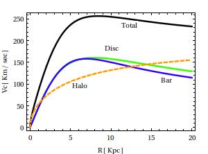
Figure 1: The rotation curve (black) corresponding to the potential $V=V_{h}+V_{d}+<V_{b}>$, where $<V_{b}>$ is the $m=0$ (average with respect to all azimuths) part of the bar’s potential $V_{b}$. The contribution of each component is shown with different color.

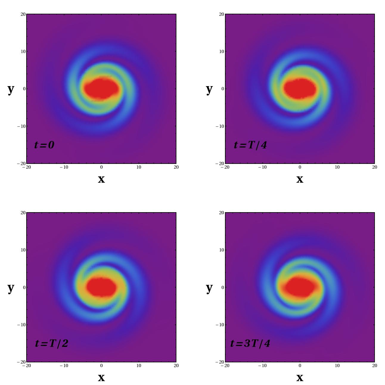
Figure 2: A color map of the surface density $\Sigma(\rho,\phi)$ corresponding to the potential $V=V_{d}+V_{b}+V_{sp}$ (see text), as viewed in the bar’s rotating frame, at four different snapshots, namely $t=0$ (top left), $t=T/4$ (top right), $t=T/2$ (bottom left) and $t=3T/4$ (bottom right), where $T=\pi/|\Omega_{sp}-\Omega_{bar}|$. Since $\Omega_{sp}<\Omega_{bar}$, the spirals have a relative clockwise angular displacement in time with respect to the bar. However, the morphological continuity between bar and spirals is retained in all these snapshots.

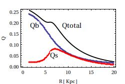
Figure 3: The bar, spiral, and total Q-strengths ($Q_{b}$, $Q_{s}$ and $Q_{total}$ respectively) as functions of the radius $\rho$ in the model including the potential terms $V_{d}$ ,$V_{b}$ and $V_{sp}$ for the ‘intermediate’ spiral model (see text).

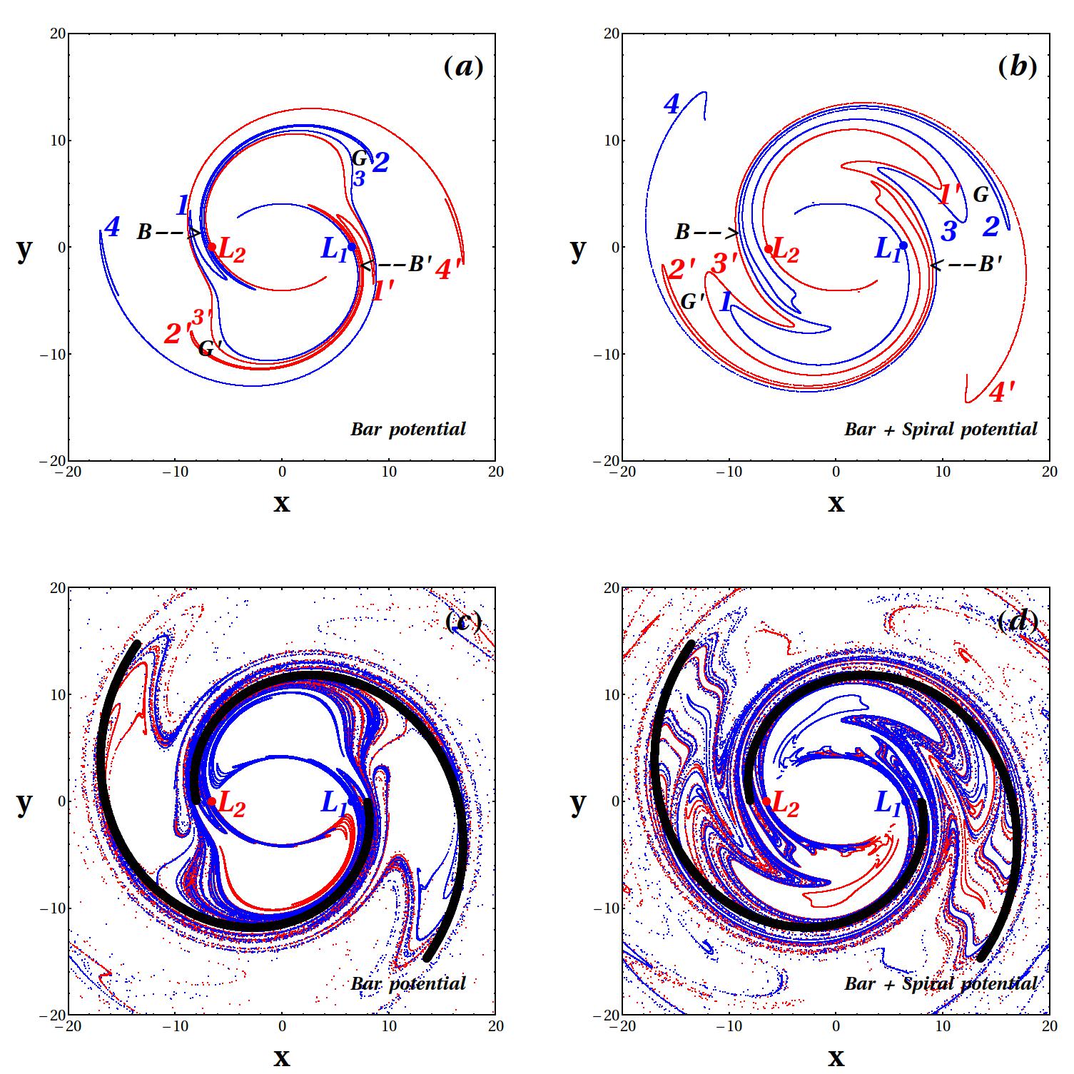
Figure 4: (a) The apocentric invariant manifolds in the pure bar model with one pattern speed. The manifolds emanating from the points $L_{1}$ and $L_{2}$ are plotted with blue and red color respectively. (b) The apocentric manifolds if we add the spiral potential (intermediate case), assuming that the spirals rotate with the same pattern speed as the bar. The addition of the spiral term enhances the structures described as ‘lobes’, ’bridges’ and ’gaps’ (see text). (c) and (d): same as in (a) and (b), but with the manifolds computed over a larger length. The black spiral curves correspond to the minima of the imposed spiral potential, given by Eq.(19).

Figure 1 shows the rotation curve arising from the axisymmetric components as well as the azimuthally averaged part of the bar’s potential (the corresponding component is equal to zero for the spirals). The model is close to ‘maximum disc’, i.e., the rotation curve up to $\sim 10$ kpc is produced essentially by the bar’s and disc components alone. On the other hand, Figure 2 shows an isodensity color map of the projected surface density $\sigma(x,y)=\int_{-\infty}^{\infty}\rho(x,y,z)dz$ in the disc plane, where the density $\rho$ is computed from Poisson’s equation $\nabla^{2}V=4\pi G\rho$ for the potential $V=V_{d}+V_{bar}+V_{sp}$. The fact that the spiral potential has a non-zero relative pattern speed in the bar’s frame results in a time-dependent spiral pattern in the disc plane. However, it is well known (Sellwood & Sparke (1988)) that, under resonable assumptions for the bar and spiral parameters, such a time dependence results in a morphological continuity, at most time snapshots, between the end of the bar and the spiral arms. For numerically testing the manifold theory, we choose below four snapshots as characteristic, corresponding to the times $t=0$, $T/4$, $T/2$ and $3T/4$ in Eq.(19), where $T=\pi/|\Omega_{sp}-\Omega_{bar}|$. Note that, since the imposed spiral potential has only $\cos 2\phi$ and $\sin 2\phi$ terms, the spiral patterns shown in Fig.2, are repeated periodically with period $T$. Defining the ‘phase’ of the spirals at a radial distance $\rho$ as the angle $\phi_{s}(\rho)$ where the spiral potential is minimum, given by

$$\phi_{s}(\rho,t)=(\Omega_{sp}-\Omega_{bar})t+(1/\tan(a))\ln(\rho/\rho_{0})~{}~{}~{}(mod2\pi),$$ (23)

we characterize below the relative position of the spirals with respect to the bar by the angle $\phi_{s}(\rho_{0},t)$, which is a periodic function of time. The angle $\phi_{s}$ is equal to the angle between the point $L_{1}$ ($L_{2}$), which, assuming the bar horizontal, lies in the semi-plane $x>0$ ($x<0$), and one of the two local minima of the spiral potential at $\rho=\rho_{0}$, which lies in the semi-plane $y\leq 0$ ($y\geq 0$).

Regarding the relative bar and spiral contributions to the non-axisymmetric forces, figure 3 allows to estimate the relative importance of the bar’s and spirals’ non-axisymmetric force perturbation by showing the corresponding Q-strengths as functions of the radial distance $\rho$ in the disc. The Q-strength at fixed $\rho$ (e.g. Buta et al (2009)) is defined for the bar as

$$Q_{b}(r)={F_{b,t}^{max}(\rho)\over<F_{r}(\rho)>}$$ (24)

where $F_{b,t}^{max}$ is the maximum, with respect to all azimuths $\phi$, tangential force generated by the potential term $V_{b}$ at the distance $\rho$, while $<F_{r}(\rho)>$ is the average, with respect to $\phi$, radial force at the same distance generated by the potential $V_{d}+V_{b}+V_{sp}$. The bar yields a Q-value $Q_{b}\approx 0.25$ in its inner part which falls to $Q_{b}\approx 0.15$ to $0.10$ in the domain outside the bar where the manifolds (and spirals) develop, i.e., $5$ kpc$<\rho<10$ kpc. The spirals, in turn, yield a maximum $Q_{s}$ around $\rho\approx 7$ kpc, equal to $Q_{s}\approx 0.08$ in the intermediate model, turning to 0.04 or 0.11 in the weak and strong models respectively. Thus, the total Q-strength is about 0.15 to 0.2 in the domain of interest.

III.2 Manifold spirals

A useful preliminary computation regards the form of the apocentric manifolds in the above models in two particular cases: i) a pure bar case, and ii) a bar+spiral case, assuming, however, the spirals to rotate with the same pattern speed as the bar. The corresponding results are shown in Fig.4. It is noteworthy that even the pure bar model yields manifolds which support a spiral response (Figs.4a,c). In addition, the manifolds induce a $R_{1}$-type ring-like structure reminiscent of ‘pseudorings’ (see Buta (2013) for a review), i.e. rings with diameter comparable to the bar’s length and a spiral-like deformation with respect to a symmetric shape on each side of the bar’s minor axis. Adding, now the spiral term (with the same pattern speed as the bar) enhances considerably these structures (Figs.4b,d). The most important effect is on the pseudo-ring structure, which is now deformed to support the imposed spirals over a large extent. It is of interest to follow in detail how the intricate oscillations of the manifolds result in supporting the imposed spiral structure. Figure 4b gives the corresponding details. We note that the manifolds emanating from the point $L_{1}$ (blue), initially expand outwards, yielding spirals with a nearly constant pitch angle. However, after half a turn, the manifolds turn inwards, moving towards the neighborhood of the point $L_{2}$. While approaching there, the manifolds develop oscillations, known in dynamics as the ‘homoclinic oscillations’ (see Contopoulos (2002)) for a review). As a result, the manifolds form thin lobes. In Figs.4a,b we mark with numbers 1 to 4 the tips of the first four lobes, and label these lobes accordingly. Focusing on Fig.4b, we note that the lobe 1 is in the transient domain between the spirals and the Lagrangian points. However, the lobe 2 of the manifold emanating from $L_{1}$ supports the spiral arm originating from the end of the bar at $L_{2}$, and, conversely, the lobe 2’ of the manifold emanating from $L_{2}$ supports the spiral arm originating from $L_{1}$. We call this phenomenon a ‘bridge’ (see also Efthymiopoulos et al. (2019)) and mark the corresponding parts of the manifolds with B and B’. One can check that this phenomenon is repeated for higher order lobes of the manifolds. Thus, in Fig.4b, the lobe 3 supports the outer part of the pseuroding assosiated with the spiral originating from $L_{2}$, while lobe 3’ supports in the same way the spiral originating from $L_{1}$. Furthermore, between lobes 2 and 3 a ‘gap’ is formed (marked G), which separates the pseudoring from the outer spiral (and similarly for the gap G’ formed between lobes 2’ and 3’). On the other hand, lobe 4 returns to support the spiral originating from $L_{1}$. Higher order lobes repeat the same phenomenon, but their succession becomes more and more difficult to follow, as shown in Fig.4d. One can remark that the manifolds support the spiral geometry mostly in the outer parts of the pseudorings. In fact, in the pure bar model we have again the appearance of manifold oscillations, leading to lobes, bridges and gaps (Figs.4a,c), but now the ring part is only mildly deformed and clearly separated from the outer lobes which support spirals.

We now examine how these morphologies are altered, if, instead, we assume the spirals to rotate with a different pattern speed than the bar. The computation of the manifolds in this case proceeds along the steps described in section 2. For the computation of the initial diagonalizing transformation matrix ${\cal A}$ (Eq.5) as well as the canonical transformation (II) we proceed as described in the Appendix. In particular, we use the Lie series method in order to perform all series computations. These series allow us to compute initial conditions for the periodic orbits $GL_{1}$ and $GL_{2}$ (Eq.(II)). Finally, we numerically refine the latter computation using Newton-Raphson to obtain the periodic orbits with many significant figures. More specifically, since the potential depends periodically on time (with period $T=\pi/(\Omega_{bar}-\Omega_{sp})$), we consider a stroboscopic map

$$(x(0),y(0),p_{\rho}(0),p_{\phi}(0))\rightarrow(x(T),y(T),p_{\rho}(T),p_{\phi}(T))$$ (25)

which maps any initial condition at the time $t=0$ to its image at the time $t=T$ under the full numerical equations of motion without any approximation. Then, the periodic orbits $GL_{1}$ and $GL_{2}$ are fixed points of the above map. As shown in Fig.5, the periodic orbits $GL_{1}$ and $GL_{2}$ found by the above method form epicycles around the Lagrangian points $L_{1}$ and $L_{2}$ of the pure bar model. However, the orbits $GL_{1}$ and $GL_{2}$ should not be confused with the epicyclic Lyapunov orbits $PL_{1}$, $PL_{2}$ used in past manifold calculations in models with one pattern speed (Voglis et al. (2006)). In particular, the orbits $PL_{1}$ and $PL_{2}$ exist as a family of orbits in a fixed bar model, whose size depends continuously on the value of the Jacobi energy $E_{J}>E_{L1}$. Under specific conditions, the orbits $PL_{1,2}$ can be generalized to 2D-tori in the case of one extra pattern speed. However, this generalization requires the use of Kolmogorov-Arnold-Moser theory (Kolmogorov (1954); Arnold (1963); Moser (1962)) which is beyond our present scope. On the contrary, in the two-pattern speed case, for a fixed choice of the potential $V_{2}=V_{sp}$ (Eq.19) and $\Omega_{2}=\Omega_{sp}$ there exist unique $GL_{1}$ and $GL_{2}$ orbits, which generalize the unique Lagrangian points of the corresponding pure bar model. In fact, the orbits of Fig.5 have relative size of the order of the ratio of the $m=2$ Fourier amplitudes of the bar and of the spiral potential at the radius $\rho=\rho_{L1,2}$. This is about $0.5$ kpc, $1.2$ kpc and $1.5$ kpc in the weak, intermediate and strong spiral case respectively.

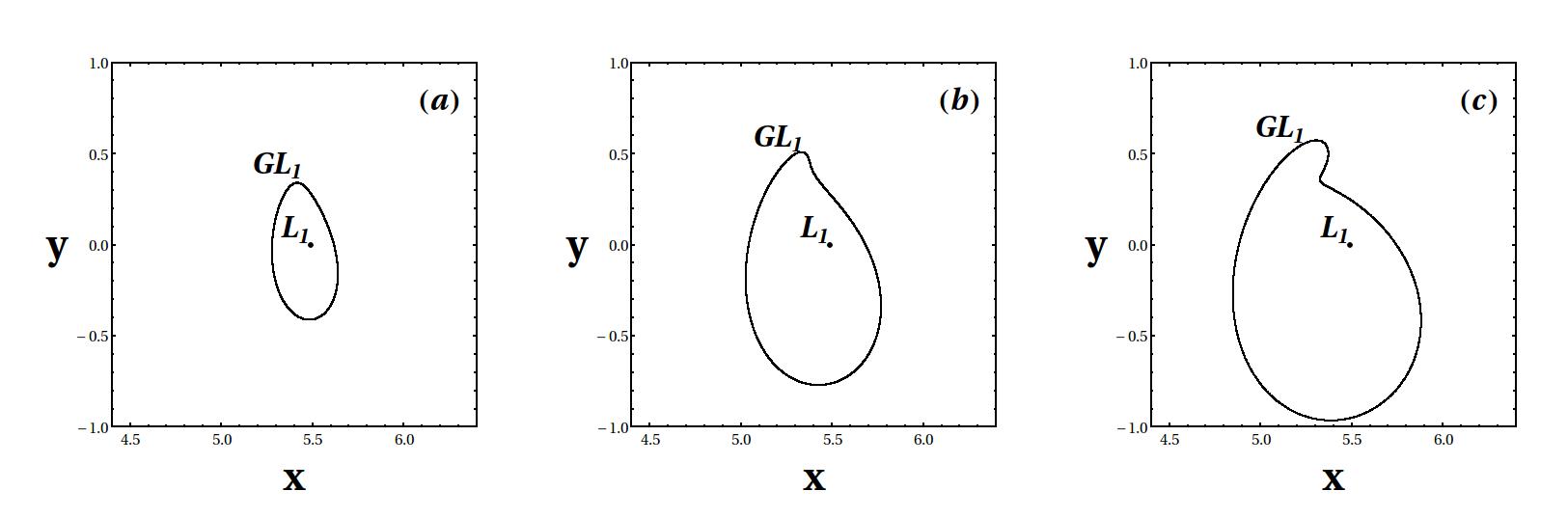
Figure 5: The periodic orbit $GL_{1}$ in the weak (left), intermediate (center) and strong (right) spiral cases. The size of the orbit increases with the spiral amplitude.

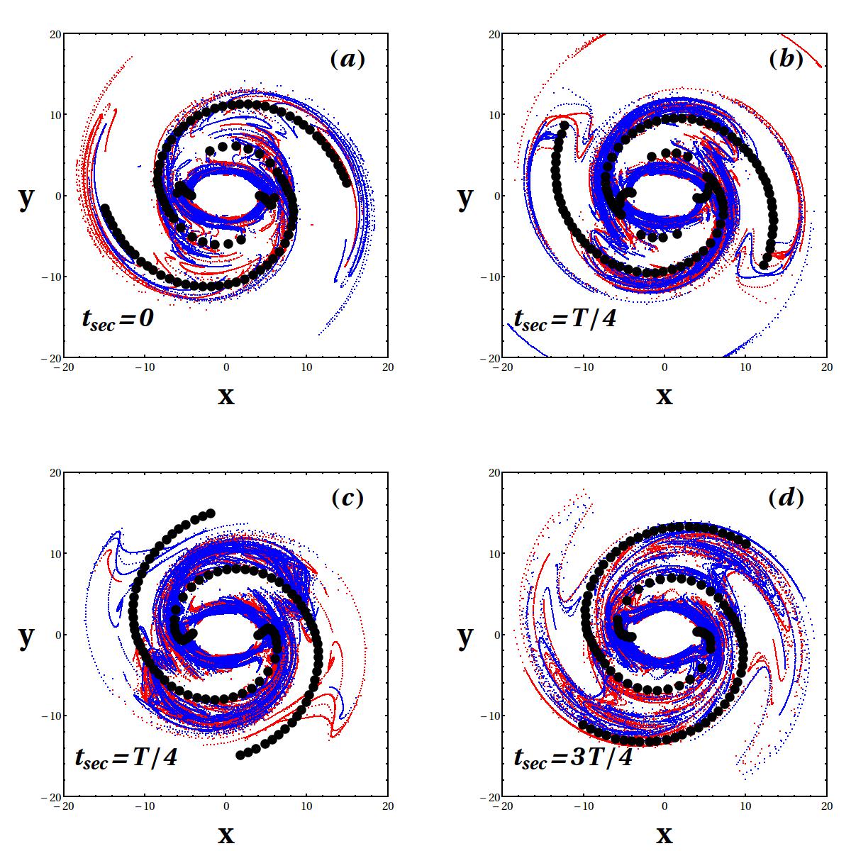
Figure 6: The ‘double section’ apocentric manifolds ${\cal W}^{AU}_{GL1}(t_{sec})$ (blue) and ${\cal W}^{AU}_{GL2}(t_{sec})$ (red) are plotted at four different times $t_{sec}$ as indicated in each panel. The black-dotted curves mark the local maxima of the surface density $\sigma(\rho,\phi,t)$ corresponding to the potential $V=V_{d}(\rho)+V_{b}(\rho,\phi)+V_{sp}(\rho,\phi,t)$ at the times $t=t_{sec}$. These maxima are plotted in the domain $6$ kpc$<\rho<15$ Kpc, where the imposed spirals have a significant amplitude.

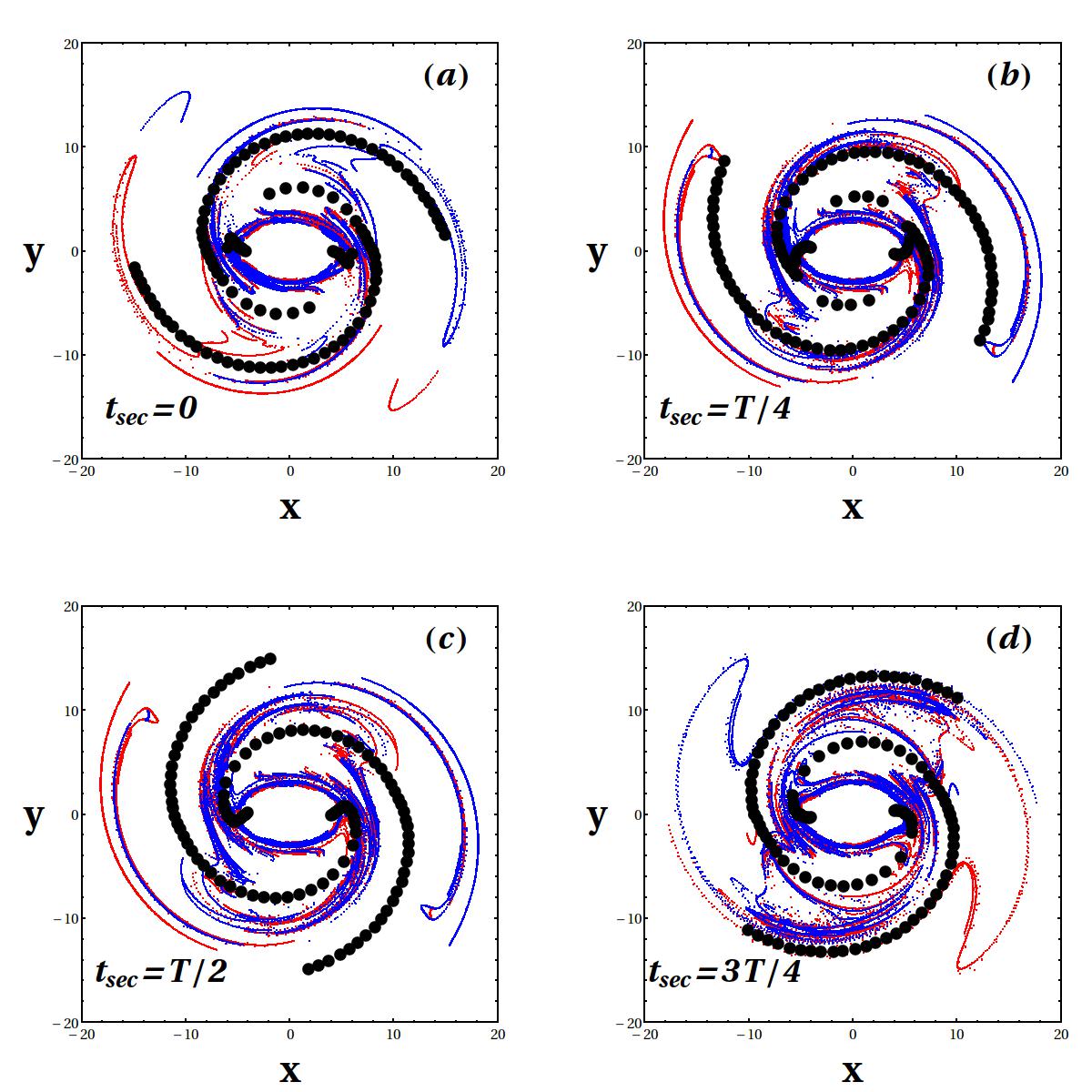
Figure 7: Same as in Fig.6, but for the weak spiral model.

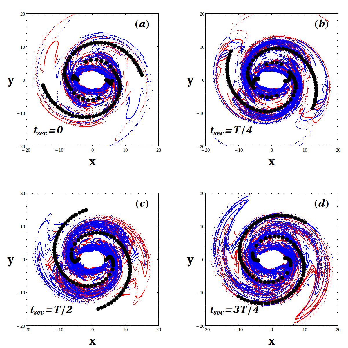
Figure 8: Same as in Fig.6, but for the strong spiral model.

The computation of the unstable manifolds of the orbits $GL_{1}$ and $GL_{2}$ is now straightforward: focusing on, say, $GL_{1}$, we first compute the $4\times 4$ variational matrix $\Lambda$ of the mapping (25) evaluated at the fixed point of the periodic orbit $GL_{1}$. The matrix $\Lambda$ satisfies the symplecticity condition $\Lambda\cdot{\cal J}\cdot\Lambda^{T}=\Lambda^{T}\cdot{\cal J}\cdot\Lambda={\cal J}$, and it has two real reciprocal eigenvalues $\lambda_{1},\lambda_{2}=1/\lambda_{1}$, with $|\lambda_{1}|>1$, and two complex congugate ones with unitary measure $\lambda_{3,4}=e^{\pm i\omega T}$ for some positive $\omega$. Denoting by $e^{U}_{GL1}$ the unitary eigenvector of $\Lambda$ associated with the eigenvalue $\lambda_{1}$, we then consider a small segment divided in $10^{5}$ initial conditions of the form $(\rho_{i,0},\phi_{i,0},p_{\rho,i,0},p_{\phi,i,0}$, $i=1,...,100000$ defined by $(\rho_{i,0},\phi_{i,0},p_{\rho,i,0},p_{\phi,i,0})=(\rho_{GL1}+\delta\rho_{i,0},\phi_{GL1}+\delta\phi_{i,0},p_{\rho,GL1}+\delta p_{\rho,i,0},p_{\phi,GL1}+\delta p_{\phi,i,0})$ where $(\delta\rho_{i,0},\delta\phi_{i,0},\delta p_{\rho,i,0},\delta p_{\phi,i,0})=(i/100000)\times\Delta S\times e^{U}_{GL1}$, with $\Delta S=0.001$. Propagating all these orbits forward in time yields an approximation of the unstable flux-tube manifold ${\cal W}^{TU}_{GL1}$ (see section 2).

In contrast to what happens in the one-pattern speed model, under the presence of the second pattern speed the projection of the ‘flux-tube’ manifolds ${\cal W}^{TU}_{GL1}$ in the disc plane varies in time. In order to efficiently visualize how the manifolds develop in space and time, in the following plots we use an apocentric double section of the manifolds, denoted ${\cal W}^{AU}_{GL1}(t_{sec})$, which depends on a chosen value of the ‘section time’ $t_{sec}$. The apocentric double section for a given time $t_{sec}$ is defined as follows: keeping track of all the points of the tube manifolds generated by the above initial conditions, we retain those points corresponding to integration times $t=nT+t_{sec}\pm\Delta T$, with $n=0,1,2,\ldots$ and $\Delta T$ small ($\Delta T=0.1T$ in all our calculations), and at the same time satisfying the apocentric condition $\dot{p}_{\rho}\simeq 0$ (with an accuracy defined by $|\dot{\rho}|<|\ddot{\rho}|dt$ where $|\ddot{\rho}|$ is the measure of the radial acceleration at the evaluation point, and $dt=0.001T$ is the integration timestep). This representation allows to obtain the intersections of the manifolds with an apocentric surface of section (see Efthymiopoulos (2010) for a discusion of how the apocentric manifolds compare with the full flux-tube manifolds). However, it also allows to capture the dependence of the form of the manifolds on time, through the chosen value of $t_{sec}$.

Figure 6 shows the main result: the manifolds ${\cal W}^{AU}_{GL1}(t_{sec})$ (blue points) and ${\cal W}^{AU}_{GL2}(t_{sec})$ (red points) computed as above, are shown at four different times $t_{sec}$, namely $t_{sec}=0$, $T/4$, $T/2$ and $3T/4$, corresponding to the same snapshots as in Fig.(2). The spiral phase $\phi_{s}(\rho_{0},t_{sec})$ has the values $0$, $-\pi/4$, $-\pi/2$ and $-3\pi/4$, respectively. The black dotted curves superposed to the manifolds correspond to the maxima of the surface density in the annulus $6~{}kpc<\rho<15~{}kpc$, as found from the data of Fig.2. These figures repeat periodically after the time $t_{sec}=T$.

The key result from Fig.6 is now evident: The spiral maxima rotate clockwise with respect to the bar (with angular velocity equal to $2\pi/(\Omega_{bar}-\Omega_{sp}$). The manifolds ${\cal W}^{AU}_{GL1,2}$ adapt their form to the rotation of the spiral maxima, thus acquiring a time-varying morphology. In particular, the manifolds always form bridges and gaps, thus supporting a pseudo-ring as well as an outer spiral pattern. The spiral-like deformation of the pseudo-ring is most conspicuous at $t_{sec}=0$, corresponding to a spiral phase $\phi_{s}(\rho_{0})=0$, and it remains large at the times $t_{sec}=T/4$ and $3T/4$, i.e., at the spiral phases $\phi_{s}(\rho_{0})=-\pi/4$ and $-3\pi/4$. At all these phases the spiral maxima at $\rho=\rho_{0}$ remain close to the bar’s major axis, thus the manifolds tend to take a form similar to the one of Fig.4d (in which $\phi_{s}(\rho_{0})=0$ always since we set $\Omega_{bar}=\Omega_{sp}$). On the other hand, at $t_{sec}=T/2$, ($\phi_{s}(\rho_{0})=-\pi/2$) the spiral maxima at $\rho=\rho_{0}$ are displaced by an angle $\pi/2$ with respect to the bar’s horizontal axis. Then, the manifolds yield more closed pseudo-rings, and they temporarily stop supporting the imposed spirals. Comparing the three phases $\phi_{s}(\rho_{0})=0$, $-\pi/4$ and $-3\pi/4$ we find that the agreement between manifolds and imposed spirals is best at the phases $\phi_{s}(\rho_{0})=0$ and $-3\pi/4$, while the manifolds support the imposed spiral mostly in their pseudo-ring part at $\phi_{s}(\rho_{0})=-\pi/4$.

Altering the spirals’ amplitude (Figs.7 and 8) makes no appreciable difference to the above picture. The main noticed difference regards the thickness of the manifolds’ lobes, which increases with the imposed spiral amplitude, since, in general, the manifolds make larger oscillations near the bridges when the non-axisymmetric perturbation increases. This means also that the trajectories supporting these spirals are more chaotic.

III.3 Discussion

Commenting on the loss of support of the manifolds to the imposed spiral maxima near $\phi_{s}(\rho_{0})=-\pi/2$, we remark that under the scenario that the manifolds provide the backbone supporting chaotic spirals, a temporary loss of support implies that the spiral response to the manifolds should have its minimum strength when the spirals have a relative phase $\pm\pi/2$ with respect to the bar’s major axis. Since the bar-spiral relative configuration (and the manifolds’ shape) is repeated periodically, with period $T=\pi/(\Omega_{bar}-\Omega_{sp})$, we conclude that under the manifold scenario the amplitude in the response spiral should exhibit periodic time variations, with a period equal to $T$, i.e., the manifolds support recurrent spirals with the above periodicity. The appearance of recurrent spirals in multi-pattern speed N-body models is well known (see Sellwood & Wilkinson (1993), Sellwood (2003)). The manifold theory provides a specific prediction about the period of the recurrence, which is testable in such experiments by the time-Fourier analysis of the non-axisymmetric patterns. On the other hand, the picture presented above is still ‘static’, in the sense that it does not take into account phenomena which alter in time the imposed non-axisymmetric modes. Such phenomena are nonlinear interactions between distinct modes, and the enhancement or decay of the spirals associated with disc instabilities (e.g. swing amplification) or with dissipation mechanisms (e.g. disc heating at resonances or gas phenomena). In all such circumstances, the manifolds provide a way to understand the behavior of chaotic trajectories beyond the bar. Thus, a full exploration of the connection between manifolds and collective disc phenomena is proposed for further study.

IV Conclusions

In the present study we have examined the possibility that manifold spirals in barred galaxies are consistent with the presence of multiple pattern speeds in the galactic disc. In section 2 we gave the main theory, and in section 3 we constructed numerical examples of such manifold spirals. Our main conclusions are the following:

1. In the case of one pattern speed, the basic manifolds are those generated by the unstable manifolds of the Lagrangian points $L_{1}$ and $L_{2}$. In the case of multiple pattern speeds, it can be established theoretically (see section 2) that, while Lagrangian equilibrium points no longer exist in the bar’s rotating frame, such points are replaced by ‘generalized Lagrangian orbits’ (the orbits $GL_{1}$ and $GL_{2}$) which play a similar role for dynamics. These orbits are periodic, with period equal to $\pi/|\Omega_{sp}-\Omega_{bar}|$, if there is one spiral pattern rotating with speed $\Omega_{sp}$ different from $\Omega_{bar}$. If there are more than one extra patterns, with speeds $\Omega_{2}$, $\Omega_{3}$, etc., the generalized orbits $GL_{1}$ and $GL_{2}$ perform epicycles around the Lagrangian points $L_{1}$ and $L_{2}$ of the pure bar model with incommensurable, in general, frequencies $|\Omega_{i}-\Omega_{bar}|$, $i=1,2,...$. Furthermore, in all cases the orbits $GL_{1}$ and $GL_{2}$ are simply unstable, a fact implying that they possess unstable manifolds ${\cal W}_{GL1}$, ${\cal W}_{GL2}$. When the extra patterns have a small amplitude with respect to the bar’s amplitude, perturbation theory establishes that the manifolds ${\cal W}_{GL1}$, ${\cal W}_{GL2}$ undergo small time variations (with the same frequencies $|\Omega_{i}-\Omega_{bar}|$, $i=1,2,...$), but their form in general exhibits only a small deformation with respect to the manifolds ${\cal W}_{L1}$, ${\cal W}_{L2}$ of the pure bar model. Thus, the manifolds ${\cal W}_{GL1}$, ${\cal W}_{GL2}$ support trailing spiral patterns.

2. In section 3 we explore a simple bar-spiral model for a galactic disc with parameters relevant to Milky-Way dynamics. In this model we construct manifold spirals in both cases of a unique pattern speed ($\Omega_{sp}=\Omega_{bar}$) or two distinct pattern speeds ($\Omega_{sp}<\Omega_{bar}$). The pure bar model already generates manifolds which support spiral patterns, and also an inner ring around the bar. Imposing further spiral perturbations in the potential generates mostly a deformation of the manifolds, with the ring evolving to a spiral-like ‘pseudo-ring’. The spiral and ring structures generated by the manifolds connect to each other through ‘bridges’ (see Figs.4,6, 7, and 8). This implies that, after a ‘bridge’, the manifold emanating from the neighborhood of the bar’s $L_{1}$ ($L_{2}$) point supports the spiral arm associated with the bar’s end near the $L_{2}$ ($L_{1}$) point. From the point of view of dynamics, these connections are a manifestation of homoclinic chaos.

3. We find that the manifold theory gives good fit to at least some part of to the imposed spirals in both the single and multiple pattern speed models. Focusing on numerical examples in which the spiral and bar pattern speeds satisfy $\Omega_{sp}<\Omega_{bar}$, the main behavior of the manifold spirals can be characterized in terms of the (time-varying) phase $\phi_{s}(\rho_{0})$ (Eq.(23)). The manifolds support the imposed spirals over all the latter’s length at phases $\phi_{s}(\rho_{0})=0$ or $-3\pi/4$, and they support mostly pseudo-ring like spirals near the phase $-\pi/4$ (the phase $\phi_{s}$ is negative since the spirals have a retrograde relative rotation with respect to the bar). On the other hand, the manifolds deviate from the imposed spirals near the phase $-\pi/2$. Both the manifolds’ shape and the imposed bar-spiral relative configuration are repeated periodically, with period $T=\pi/(\Omega_{bar}-\Omega_{sp})$. Thus, we argued that the temporary loss of support of the manifolds to the imposed spirals suggests a natural period for recurrent spirals, equal to $T$.

In summary, our analysis shows that manifold spirals in galactic discs are, in general, consistent, with the presence of multiple pattern speeds. Nevertheless, the manifold spirals in this case oscillate in time, thus, they support the imposed spirals along a varying length, which fluctuates from small to almost complete, depending on the relative phase of the spirals with respect to the bar. The manifolds also produce ring and pseudo-ring structures, morphologically connected to the spirals via the phenomenon of ‘bridges’ (section 3). These features are present in real galaxies (Buta (2013)), but testing their connection to manifolds in specific cases of galaxies requires a particular study.

Acknowledgements: We acknowledge support by the Research Committee of the Academy of Athens through the grant 200/895. C.E. acknowledges useful discussions with Dr. E. Athanassoula.

Appendix A Series construction

Starting from the Hamiltonian (II), we implement the method of composition of Lie series in order to arrive to the Hamiltonian (II), by the following steps:

1) Expansion: We compute the Lagrangian points $L_{1}$, $L_{2}$ of the Hamiltonian (3). Selecting, say, the point $L_{1}$, with co-ordinates $\rho_{L1},\phi_{L_{1}},0,p_{\phi,L1}$, we expand the full Hamiltonian (II) in a polynomial series in the variables $\delta\rho=\rho-\rho_{L1}$, $\delta\phi=\phi-\phi_{L1}$, $J_{\phi}=p_{\phi}-p_{\phi,L1}$ (see section 2). In a computer-algebraic implementation, all expansions are carried up to a maximum truncation order $N_{t}$, set as $N_{t}=10$.

2) Diagonalization: From the quadratic part $H_{0,2}$ of the Hamiltonian we compute the variational matrix ${\cal M}$ at $L_{1}$, as in Eq.(7), as well as its eigenvalues $\lambda_{1,3}=\pm\nu$, $\lambda_{2,4}=\pm i\kappa$, with $\nu,\kappa>0$, and associated eigenvectors $e_{i}$, $i=1,\ldots,4$. Each eigenvector has four components, thus it can be written as a $4\times 1$ column vector. We then form the $4\times 4$ matrix ${\cal B}=(c_{1}e_{1},c_{2}e_{2},c_{1}e_{3},c_{2}e_{2})$, with unspecified coefficients $c_{1},c_{2}$, which contains the four vectors as its columns (multiplied by the $c_{i}$’s). Applying the symplectic condition ${\cal B}^{T}\cdot{\cal J}\cdot{\cal B}={\cal J}$, where ${\cal J}_{4}$ is the $4\times 4$ fundamental symplectic matrix

$${\cal J}_{4}=\begin{bmatrix}0&I_{2}\\ -I_{2}&0\\ \end{bmatrix}$$ (26)

with $I_{2}$ equal to the $2\times 2$ identity matrix, yields two independent equations allowing to specify the coefficients $c_{1},c_{2}$, and hence all the entries of the constant matrix ${\cal B}$. This matrix ${\cal A}$ in the transformation (5) is then given by ${\cal A}={\cal B}\cdot{\cal C}$ where

$${\cal C}=\begin{bmatrix}1&0&0&0\\ 0&{1\over\sqrt{2}}&0&{-i\over\sqrt{2}}\\ 0&0&1&0\\ &-{i\over\sqrt{2}}&0&{1\over\sqrt{2}}&0\\ \end{bmatrix}$$ (27)

3) Normalization using Lie series: We use the Lie method of normal form construction (see Efthymiopoulos (2012) section 2.10 for a tutorial) in order to pass from the Hamiltonian (II) to the Hamiltonian (II). Briefly, we consider a sequence of canonical transformations $(u^{(r-1)},Q^{(r-1)},v^{(r-1)},P^{(r-1)})$ $\rightarrow$ $(u^{(r)},Q^{(r)},v^{(r)},P^{(r)})$, with $r=1,2,\ldots,N_{t}$, where $(u^{(0)},Q^{(0)},v^{(0)},P^{(0)})$ $\equiv$ $(u,Q,v,P)$ and $(u^{(N_{t})},Q^{(N_{t})},v^{(N_{t})},P^{(N_{t})})$, $\equiv$ $(\xi,q,\eta,p)$ defined through suitably defined generating functions $\chi_{1},\chi_{2},\ldots,\chi_{N_{t}}$, through the recursive relations

$$(u^{(r-1)},Q^{(r-1)},v^{(r-1)},P^{(r-1)})=~{}~{}~{}~{}~{}~{}~{}~{}~{}~{}~{}~{}~{}~{}~{}$$ (28)

$$~{}~{}~{}~{}~{}~{}~{}~{}~{}~{}~{}~{}~{}~{}~{}~{}~{}\exp\left({\cal L}_{\chi_{r}}\right)(u^{(r)},Q^{(r)},v^{(r)},P^{(r)})$$

where ${\cal L}_{\chi_{r}}$ denotes the Poisson bracket operator ${\cal L}_{\chi_{r}}\cdot=\{\cdot,\chi_{r}\}$, and $\exp({\cal L}_{\chi_{r}})=\sum_{j=0}^{\infty}{\cal L}_{\chi_{r}}^{j}/j!$ (truncated at order $N_{t}$. Once the involved generating functions $\chi_{r}$ $r=1,2,\ldots,N_{t}$ are specified, Eq.(28) allows to define the transformation of Eq.(II), and hence the periodic orbit $GL_{1}$ through Eq.(II).

It remains to see how to compute the functions $\chi_{r}$. This is accomplished via a recursive algorithm, allowing to transform the original Hamiltonian $H^{(0)}\equiv H$, with $H$ given by Eq.(II) to its final form $H^{(N_{t})}$ given by Eq.(II). We consider the $r-$th normalization step, and give explicit formulas in the case of one extra pattern speed, in which we have one extra angle $\phi_{2}=\phi_{s}$ (generalization to $M$ extra pattern speeds is straightforward). The Hamiltonian has the form

$$H^{(r-1)}=Z_{2}+Z_{3}+...+Z_{r+1}+R_{r+2}^{(r-1)}+\ldots+R_{N_{t}+2}^{(r-1)}$$ (29)

where i) subscripts refer to polynomial order in the variables $(u^{(r-1)},Q^{(r-1)},v^{(r-1)},P^{(r-1)})$, and ii) the terms $Z_{i}$, $i=2,\ldots,r+1$ are ‘in normal form’, i.e., contain no monomials linear in $(u^{(r-1)},v^{(r-1)})$. The remainder term $R_{r+2}^{(r-1)}$ has the form

$$R_{r+2}^{(r-1)}=\sum_{m}\sum_{k_{1}+k_{2}+l_{1}+l_{2}=r+2}a_{k_{1},k_{2},l_{1},l_{2}}^{(r-1)}$$

$$\times e^{im\phi_{s}}(u^{(r-1)})^{k_{1}},(Q^{(r-1)})^{k_{2}},(v^{(r-1)})^{l_{1}},(P^{(r-1)})^{l_{2}}$$

with $k_{1},k_{2},l_{1},l_{2}\geq 0$, and $m$ integer. Then, the generating function $\chi_{r}$ is given by

$$\chi_{r} = \sum_{k_{1}+l_{1}=1}a_{k_{1},k_{2},l_{1},l_{2}}^{(r-1)}$$

$$\times {e^{im\phi_{s}}(u^{(r)})^{k_{1}},(Q^{(r)})^{k_{2}},(v^{(r)})^{l_{1}},(P^{(r)})^{l_{2}}\over(l_{1}-k_{1})\nu+i[(k_{2}-l_{2})\kappa+m(\Omega_{s}-\Omega_{bar})]}~{}~{}.$$

With the above rule, the Hamiltonian becomes ‘in normal form’ up to the terms of polynomial order $r+2$, namely

$$H^{(r)} = \exp({\cal L}_{\chi_{r}})H^{(r-1)}$$

$$= Z_{2}+Z_{3}+...+Z_{r+2}+R_{r+3}^{(r)}+\ldots+R_{N_{t}+2}^{(r)}~{}~{}.$$

Hence, repeating the procedure $N_{t}$ times leads to the Hamiltonian (II).

References

- Antoja et al. (2014) Antoja, T, Helmi, A., Dehnen, W., et al.: 2014, A&A, 563, 60
- Arnold (1963) Arnold, V.I. 1963, Russ. Math. Surveys, 18, 9
- Athanassoula et al. (2009a) Athanassoula, E., Romero-Gómez, M., Masdemont, J. J.: 2009a, MNRAS, 394, 67
- Athanassoula et al. (2009b) Athanassoula, E., Romero-Gómez, M., Bosma, A., Masdemont, J.J.: 2009b, MNRAS, 400, 1706
- Athanassoula (2012) Athanassoula, E.: 2012, MNRAS, 426, L46
- Baba et al. (2013) Baba, J., Saitoh, T.R., Wada, K.: 2013, ApJ, 763, 46
- Baba (2015) Baba, J.: 2015, MNRAS, 454, 2954
- Binney & Tremaine (2008) Binney J., and Tremaine S.: 2008, Galactic Dynamics, second edn. Princeton University Press
- Binney (2013) Binney, J.: 2013, in ‘Secular Evolution of Galaxies’, XXIII Canary Islands Winter School of Astrophysics. J Falcon-Barroso and J. H. Knapen (eds), Cambridge University Press, pp.259-304.
- Bland-Hawthorn & Gerhard (2016) Bland-Hawthorn, J., and Gerhard, O.: 2016, Annu. Rev. A&A Astrophys., 54, 529
- Boonyasait et al. (2005) Boonyasait, V., Patsis, P.A., and Gottesman, S.T: 2005, NYASA, 1045, 203
- Buta et al (2009) Buta, R.J., Knapen, J.H., Elmegreen, B.G., Salo, H., Laurikainen, E., Elmegreen, D.M., Puerari, I., Block, D.L.: 2009, AJ, 137, 4487
- Buta (2013) Buta, R.: 2013, in ‘Secular Evolution of Galaxies’, XXIII Canary Islands Winter School of Astrophysics. J Falcon-Barroso and J. H. Knapen (eds), Cambridge University Press, pp…..
- Cao et al (2013) Cao, L., Mao, S., Nataf, D., Rattenbury, N.J., and Gould, A.: 2013, MNRAS, 434, 595
- Contopoulos (2002) Contopoulos,G.: 2002, ‘Order and Chaos in Dynamical Astronomy’, Springer
- Cox & Gómez (2002) Cox, D.P., and Gómez, G.C.: 2002, ApJS, 142, 261
- Danby (1965) Danby, J.M.A., 1965: AJ, 70, 501
- Dehnen (1993) Dehnen, W.: 1993, MNRAS, 265, 250D
- Diaz-Garcia et al (2019) Díaz-García, S., Salo, H., Knapen, J.H., Herrera-Endoqui, M.: 2019, arXiv190804246D
- Dubinski et al. (2009) Dubinski, J., Berentzen, I., and Shlosman, I.: 2009, ApJ 697, 293
- Efthymiopoulos (2010) Efthymiopoulos, C., 2010: Eur. Phys. J. Special Topics, 186, 91
- Efthymiopoulos (2012) Efthymiopoulos, C.: 2012, In Cincotta P.M., Giordano C.M., Efthymiopoulos C. (eds.) “Third La Plata Internat. School on Astron. Geophys.”, Asociación Argentina de Astronomía, La Plata
- Efthymiopoulos et al. (2019) Efthymiopoulos, C., Kyziropoulos, P., Paez, R., Zouloumi, K., and Gravvanis, G.: 2019: MNRAS 484, 1487
- Font et al. (2014) Font, J., Beckman, J.E., Querejeta, M., Epinat, B., James, P.A., Blasco-herrera, J., Erroz-Ferrer, S., Pérez, I.: 2014, ApJS, 210, 2
- Font et al. (2019) Font, J, Beckman, J., James, P.A., and Patsis, P.A.: 2019, MNRAS, 482, 5362
- Gerhard (2002) Gerhard, O.: 2002, in Da Costa, G.S., Sadler, E.M., and Jerjen, H. (eds), “The Dynamics, Structure and History of Galaxies: A Workshop in Honour of Professor Ken Freeman”, Astronomical Society of the Pacific Conference Series, p.
- Gerhard (2011) Gerhard, O.: 2011, “Pattern speeds in the Milky Way”, Mem. Soc. Astron. It. Sup., 18, 185.
- Giorgilli (2001) Giorgilli, A.: 2001, Discrete Contin. Dyn. Syst. 7, 855
- Gómez et al (2001) Gómez, G., Jorba, A., Masdemont, J., Simó, C.: 2001, “Dynamics andMission Design near Libration Points, Vol. IV”, Advanced Methods for Triangular Points, Ch. 3. World Scientific, Singapore
- Grobman (1959) Grobman, D.M.: 1959, Dokl. Akad. Nauk SSSR 128, 880
- Harsoula et al. (2016) Harsoula, M., Efthymiopoulos, C., and Contopoulos, G.: 2016, MNRAS, 459, 3419
- Hartman (1960) Hartman, P.: 1960, Proc. Amer. Math. Soc. 11, 610
- Kalnajs (1973) Kalnajs, A.J.: 1973, Pub. Astron. Soc. Australia, 2, 174
- Junqueira et al. (2015) Junqueira, T.C., Chiappini, C., L epine, J.R.D., Minchev, I., Santiago, B.X.: 2015, MNRAS 449, 2336
- Kolmogorov (1954) Kolmogorov, A.N.: 1954, Dokl. Akad. Nauk SSSR, 98, 527
- Lin & Shu (1964) Lin, C.C., and Shu, F.: 1964, ApJ, 140, 646
- Little & Carlberg (1991) Little, B., and Carlberg, R.G.: 1991, MNRAS, 250, 161
- Long & Murali (1992) Long, K., and Murali, C.: 1992, ApJ, 397, 44L
- Meidt et al. (2009) Meidt, S.E., Rand, R.J., and Merrifield, M.R.: 2009, ApJ, 702, 277
- Minchev & Quillen (2006) Minchev, I., and Quillen, A.C.: 2006, MNRAS, 368, 623
- Minchev et al. (2012) Minchev, I., Famaey, B., Quillen, A.C., Di Matteo, P., Combes, F., Vlajić, M., Erwin, P., Bland-Hawthorn, J.: 2012, A&A, 548, 126
- Miyamoto & Nagai (1975) Miyamoto, M., and Nagai, R.: 1975, PASJ, 27, 533
- Moser (1962) Moser, J.: 1962, Nachr. Akad. Wiss. Göttingen, Math. Phys. Kl II, 1-20
- Patsis (2006) Patsis, P.: 2006, MNRAS, 369, L56
- Patsis et al. (2009) Patsis, P.A., Kaufmann, D.E., Gottesman, S.T.and Boonyasait, V.: 2009, MNRAS, 394, 142
- Pettitt et al. (2014) Pettitt, A.R., Dobbs, C.L., Acreman, D.M., and Price, D.J.: 2014, MNRAS 444, 919
- Quillen (2003) Quillen, A.C.: 2003, ApJ, 125, 785
- Quillen et al. (2011) Quillen, A.C., Dougherty, J., Bagley, M.B., Minchev, I., Comparetta, J.: 2011, MNRAS, 417, 762
- Rattenbury et al (2007) Rattenbury, N.J., Mao, S., Sumi, T., and Smith, M.C.: 2007, MNRAS, 378, 1064
- Rautiainen & Salo (1999) Rautiainen, P., Salo, H.: 1999, A&A, 348, 737
- Roca-Fabrega et al. (2013) Roca-Fàbrega, S, Valenzuela, O., Figueras, F., Romero-Gómez, M., Vel’azquez, H., Antoja, T., Pichardo, B: 2013, MNRAS, 432, 2878
- Romero-Gomez et al. (2006) Romero-Gomez, M., Masdemont, J.J., Athanassoula, E. and Garcia-Gomez, C.: 2006, A&A, 453, 39
- Romero-Gomez et al. (2007) Romero-Gomez, M., Athanassoula, E., Masdemont, J.J. and Garcia-Gomez, C.: 2007, A&A, 472, 63
- Sellwood & Sparke (1988) Sellwood, J.A., and Sparke, L.S.: 1988, MNRAS, 231, 25
- Sellwood & Wilkinson (1993) Sellwood, J.A., Wilkinson, A.: 1993, RPPh, 56, 173
- Sellwood (2003) Sellwood, J. A. 2003, ApJ, 587, 638
- Sellwood (2014) Sellwood, J.A.: 2014, RvMP, 86, 1
- Speights and Westpfahl (2012) Speights, J.C., and Westpfahl, D.J.: 2012, ApJ, 752, 52
- Speights & Rooke (2016) Speights, J.C., and Rooke, P.: 2016, ApJ, 826, 2
- Tsoutsis et al. (2008) Tsoutsis, P., Efthymiopoulos, C. and Voglis, N.: 2008, MNRAS, 387, 1264
- Tsoutsis et al. (2009) Tsoutsis, P., Kalapotharakos, C., Efthymiopoulos, C. and Contopoulos, G.: 2009, A&A, 495, 743
- Vera-Villamizar et al. (2001) Vera-Villamizar, N., Dottori, H., Puerari, I., and de Carvalho, R.: 2001, ApJ, 547, 187
- Voglis et al. (2006) Voglis, N., Tsoutsis, P. and Efthymiopoulos, C.: 2006a, MNRAS, 373, 280
- Wiggins (1990) Wiggins, S.: 1990, ‘Introduction to Nonlinear Dynamical Systems and Chaos’, Springer, New York
- Wiggins (1994) Wiggins, S.: 1994, “Normally hyperbolic invariant manifolds in dynamical systems”, Springer-Verlag, New York