Level 1 Track Finder at CMS

Andrew Hart
for the CMS Tracker Group

Department of Physics and Astronomy
Rutgers, The State University of New Jersey, Piscataway, NJ, USA

Abstract: The High-Luminosity LHC is expected to deliver proton-proton collisions every 25 ns with an estimated 140–200 pileup interactions per bunch crossing. Ultrafast track finding is vital for handling Level 1 trigger rates in such conditions. An FPGA-based track trigger system, capable of finding tracks with momenta above 2 GeV, is presented.

Talk presented at the 2019 Meeting of the Division of Particles and Fields of the American Physical Society (DPF2019), July 29–August 2, 2019, Northeastern University, Boston, C1907293.

1 Introduction

The High-Luminosity LHC is expected to achieve luminosities up to $5\times 10^{34}\,\text{cm}^{-2}\text{s}^{-1}$, or up to $7.5\times 10^{34}\,\text{cm}^{-2}\text{s}^{-1}$ in the ultimate performance scenario. This amount of data offers great opportunities in terms of potential physics results. However, the pileup associated with this luminosity is at the level of 140–200 interactions per bunch crossing, presenting serious challenges at all stages of data collection and analysis.

Providing tracks to the Level 1 (L1) trigger [1] is a key part of the strategy that CMS [2] will employ to cope with the high amounts of pileup [3, 4]. Tracks at L1 will help mitigate the effects of pileup in several ways, e.g., increasing the purity of L1 muons by requiring an associated L1 track, thus reducing background rates (see the left plot of Figure 1). They will also help improve the measurement of muons and other objects that have tracks (see the right plot of Figure 1). Finally, L1 tracks open up possibilities for new kinds of triggers that are currently impossible, e.g., those based on displaced or disappearing tracks [5].

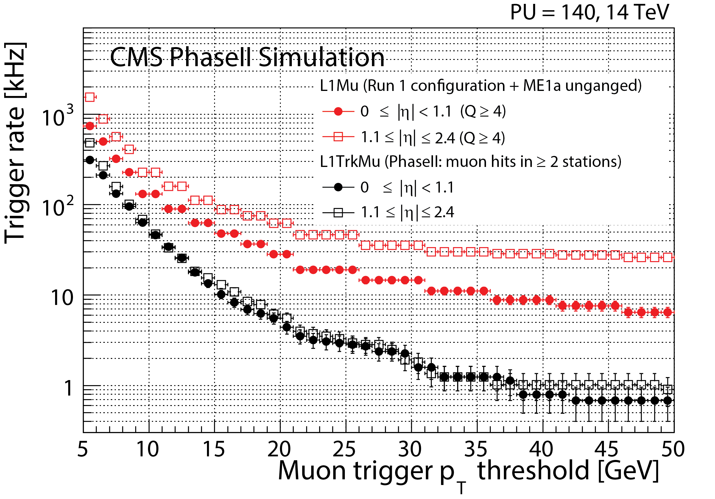
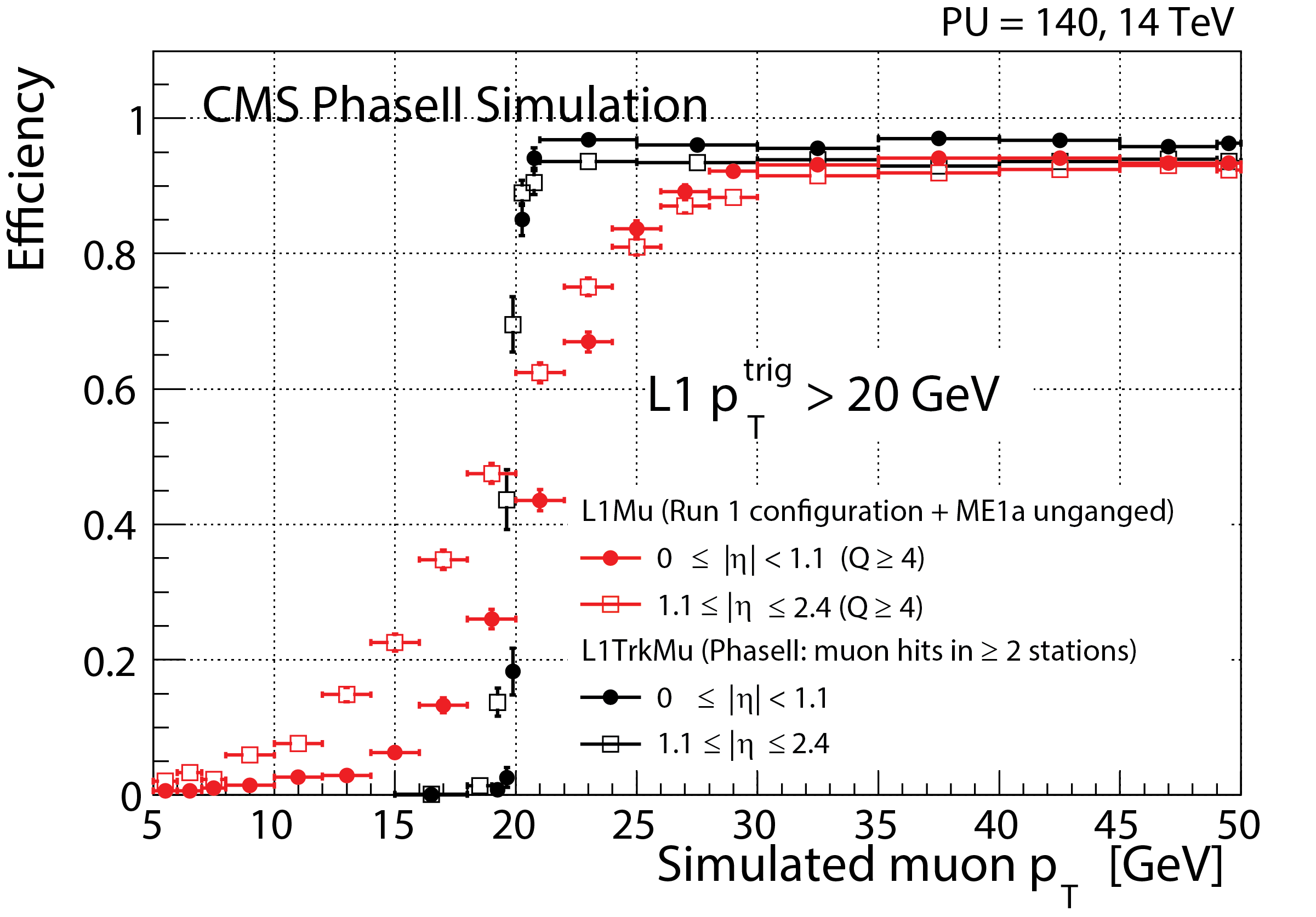
Figure 1: Trigger rates versus muon trigger $p_{\text{T}}$ threshold (left) and trigger efficiencies versus simulated muon $p_{\text{T}}$ (right) for a single-muon trigger without (red points) and with (black points) L1 tracks [3].

Two all-FPGA track trigger algorithms have been developed by CMS, which differ in their approaches to both pattern recognition and track fitting. The tracklet algorithm employs a straightforward road search for pattern recognition, followed by a simple, linearized $\chi^{2}$ fit. On the other hand, the time-multiplexed track finder (TMTT) algorithm uses a Hough transform to find tracks, and a Kalman filter to fit the tracks that are found. Both approaches have achieved similar track-finding efficiencies and track parameter resolutions in emulation, as can be seen in Figures 2 and 3. Furthermore, technical demonstrations in 2016 proved the feasibility of both approaches in hardware.

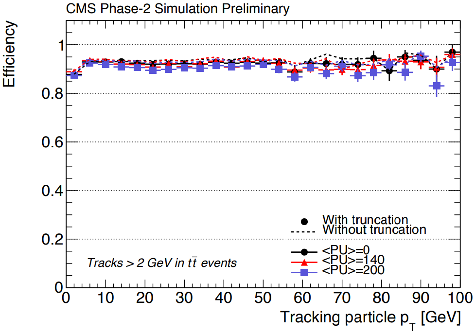
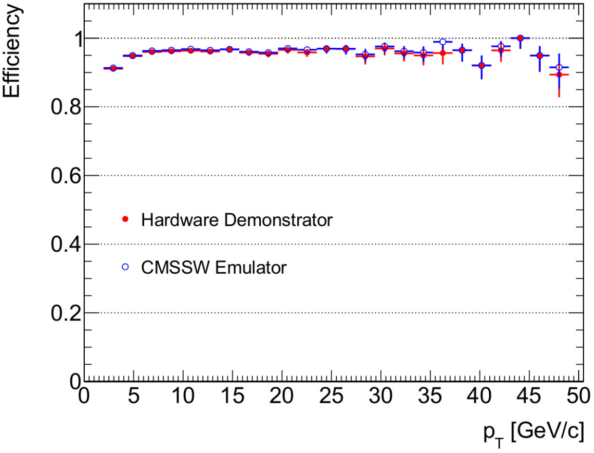
Figure 2: L1 tracking efficiencies versus simulated particle $p_{\text{T}}$ for the tracklet algorithm (left) and the TMTT algorithm (right).

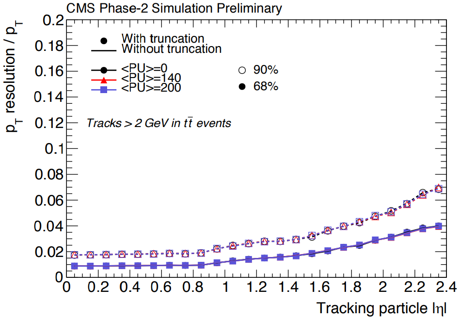
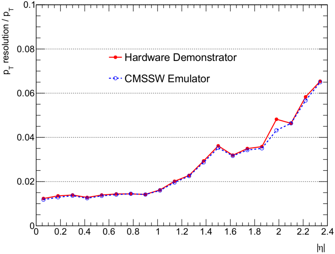
Figure 3: Relative transverse momentum resolutions versus simulated particle $|\eta|$ for L1 tracks produced by the tracklet algorithm (left) and the TMTT algorithm (right).

The current focus now is on a hybrid algorithm that combines the most sophisticated parts of the two approaches: using a road search for pattern recognition and a Kalman filter for track fitting. This algorithm will be outlined in this talk.

2 Track trigger algorithm

Track finding begins with track stubs that are formed by two types of $p_{\text{T}}$ modules, each of which contains two layers of active material with a small gap between. In the pixel-strip modules, one of the layers is composed of $1.5\,\text{mm}\times 100\,\mu\text{m}$ pixels while the other layer is a strip sensor with a $100\,\mu\text{m}$ strip pitch. These modules will be used closer to the interaction point, where the higher occupancy demands finer segmentation. Farther from the interaction point, strip-strip modules will be used, where both layers of active material are strip sensors with a pitch of $90\,\mu\text{m}$. The two-sided nature of the modules allows for front-end $p_{\text{T}}$ discrimination. As illustrated in Figure 4, stubs with too low $p_{\text{T}}$ are rejected, which results in a data reduction factor of 10–100.

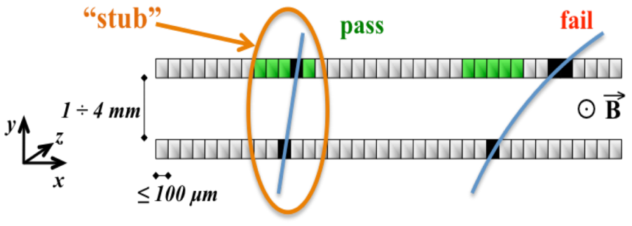
Figure 4: Illustration of the $p_{\text{T}}$ discrimination capabilities of the two-sided $p_{\text{T}}$ modules. The stub on the left is consistent with the chosen $p_{\text{T}}$ threshold and is read out by the front-end, while the stub on the right is not.

The track-finding algorithm that proceeds after stub formation is parallelized, both in time and space. It is time-multiplexed with a factor of 18 in the current design, and the tracker is divided into nine “hourglass” sectors, with an independent instance of the algorithm processing the stubs from each sector. The hourglass shape, shown in Figure 5, prevents tracks with a $p_{\text{T}}$ above a certain threshold from entering more than one sector, thus eliminating the need for cross-sector communication of tracks. The critical radius ($R^{*}$ in the figure), is a parameter that is tuned to minimize the overlap regions between sectors in which stub data must be duplicated.

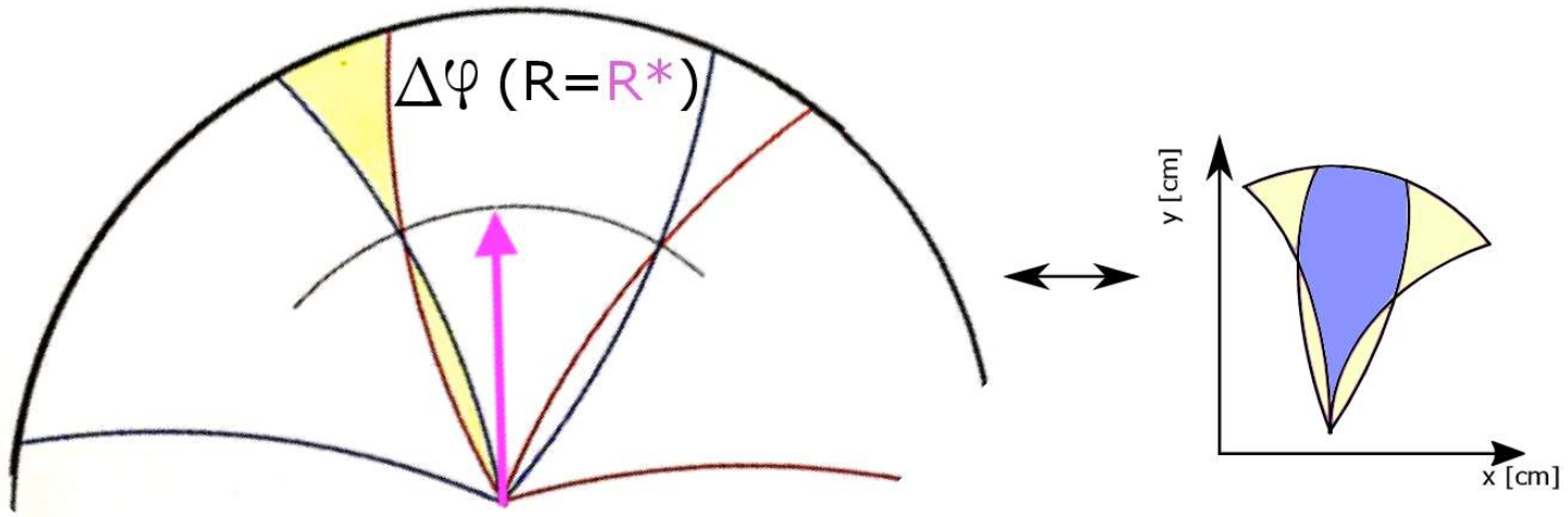
Figure 5: Hourglass sector shape used to divide the tracker for the purpose of parallelizing the track-finding algorithm. The yellow region is shared by neighboring sectors, and stubs in this region must be duplicated. However, the curved edges of the sector are such that tracks with $p_{\text{T}}$ above a certain threshold can appear in only one sector.

Once stubs are formed, track finding begins in each sector by finding pairs of stubs in adjacent tracker layers that are consistent with a track. These stub pairs act as seeds from which full tracks are grown. To reduce the volume of data that has to be processed in subsequent steps, only stub pairs consistent with $p_{\text{T}}>2\,\text{GeV}$ are kept. This is achieved by coarsely segmenting the tracker layers into virtual modules (VM), 16 or 32 per layer per sector, as illustrated in Figure 6. Then, only VM pairs consistent with the $p_{\text{T}}$ threshold of 2 GeV are connected in the firmware, with all other combinations being ignored. Similarly, the tracker is segmented into eight bins in the longitudinal direction, and only stubs in combinations of bins that are consistent with a track originating from near the nominal interaction point are considered for pairing.

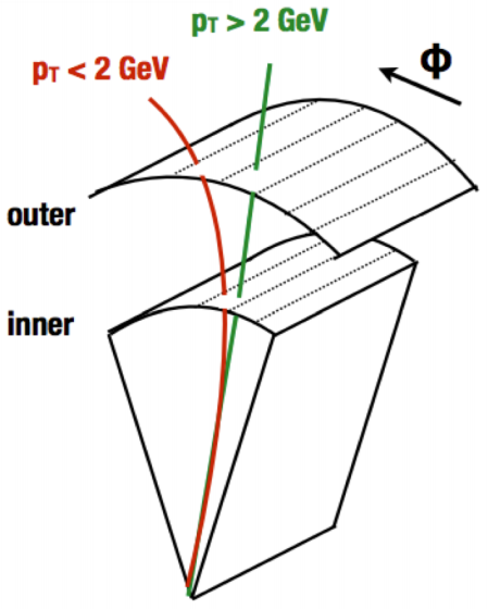
Figure 6: Illustration of the $p_{\text{T}}$ discrimination applied when forming stub pairs. The green track produces stubs in VMs that are considered for pairing, while the red track does not.

After the track seeds are found, the helix parameters and projections to other tracker layers are calculated for these “tracklets,” assuming they originate from the beamline. The projections are used to calculate residuals and match stubs in additional layers, which yields full tracks that can then be fit. The processes of seeding, calculating projections, and matching additional stubs are illustrated in Figure 7.

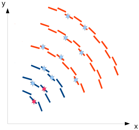
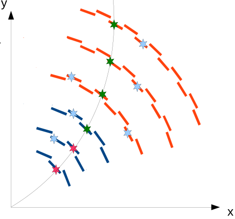
Figure 7: Illustrations of the processes of seeding, calculating projections, and matching additional stubs. The red stars in the two innermost layers of the leftmost illustration indicate a stub pair that will be used to seed a track. Projections to the other four layers are calculated in the middle illustration. Finally, the green stars in the rightmost illustration indicate additional stubs that are matched to the track based on their residuals with respect to the projections.

However, the pattern recognition naturally produces several duplicate tracks for a given charged particle. Most come from redundancies in the seeds that are used to maximize track-finding efficiency; i.e., a given charged particle will typically be seeded multiple times in different pairs of adjacent tracker layers, resulting in multiple tracks for the same particle. A few also come from nearby stubs in a given layer yielding very similar tracks, a scenario illustrated in Figure 8. Whatever the origin, these duplicate tracks have to be removed before track fitting to reduce the processing required for that step, and the current strategy is to merge any tracks that share at least four stubs, although this is an active area of development.

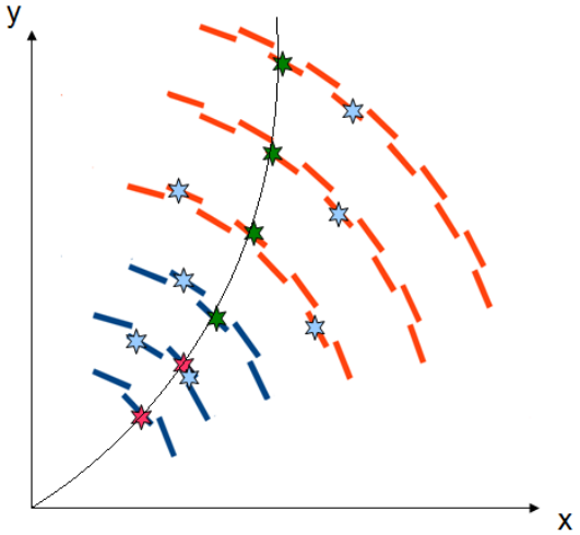
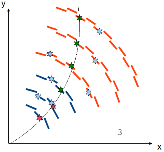
Figure 8: Two distinct tracks resulting from the same charged particle. The two tracks are identical except for the stub in the second layer, where there is ambiguity.

The final fit of the tracks is done with a Kalman filter. The filter starts with the coarse helix parameters that were calculated previously for the tracklet seed. Then stubs are added one by one, as the helix parameters are updated with greater and greater precision. Currently, there is a beamline constraint and only four parameters are fit. However, the possibility of removing this constraint and also fitting for the transverse impact parameter is being investigated.

3 Firmware status

For firmware development, we have chosen to employ Vivado High-Level Synthesis (HLS) from Xilinx. This allows FPGA designs to be written in C++ instead of a traditional HDL such as Verilog or VHDL. This enables more rapid development, especially by individuals who may not have experience writing firmware. Also, the result should be easier to maintain, and new ideas can be prototyped more easily.

The current design is divided into nine processing modules, with multiple instances of each module being employed in the design, and with memories used to communicate the results between steps. Nearly all of these have at least one instance written and tested to be functionally correct, and additional instances will be generated using C++ template programming. Of those that have been written, nearly all have achieved the desired pipelining, and about half (four of the nine modules) have been fully verified with C/RTL cosimulation. This means that, for these modules, the RTL generated by Vivado HLS produces results that agree exactly with the C++ source code. The goal is to have a full chain of modules ready for integration tests at CERN in the autumn of 2019.

4 Conclusion

A common Level 1 tracking algorithm for the CMS upgrade for the High-Luminosity LHC is under development. It is a hybrid algorithm based on the most sophisticated aspects of two proven all-FPGA approaches: tracklet and time-multiplexed track finder. Development of the firmware with Vivado High-Level Synthesis is well underway with about half of the processing steps having fully verified modules written, with a full chain expected to be ready for integration tests at CERN in the autumn of 2019.

References

- [1] V. Khachatryan et al. [CMS Collaboration], “The CMS trigger system,” JINST 12, no. 01, P01020 (2017) doi:10.1088/1748-0221/12/01/P01020 [arXiv:1609.02366 [physics.ins-det]]
- [2] S. Chatrchyan et al. [CMS Collaboration], “The CMS Experiment at the CERN LHC,” JINST 3, S08004 (2008) doi:10.1088/1748-0221/3/08/S08004
- [3] D. Contardo, M. Klute, J. Mans, L. Silvestris and J. Butler, “Technical Proposal for the Phase-II Upgrade of the CMS Detector,” CERN-LHCC-2015-010, LHCC-P-008, CMS-TDR-15-02
- [4] K. Klein, “The Phase-2 Upgrade of the CMS Tracker,” CERN-LHCC-2017-009, CMS-TDR-014
- [5] CMS Collaboration [CMS Collaboration], “First Level Track Jet Trigger for Displaced Jets at High Luminosity LHC,” CMS-PAS-FTR-18-018, http://cds.cern.ch/record/2647987
- [6] R. Aggleton et al., “A novel FPGA-based track reconstruction approach for the level-1 trigger of the CMS experiment at CERN,” doi:10.23919/FPL.2017.8056825
- [7] E. Bartz et al., “FPGA-Based Tracklet Approach to Level-1 Track Finding at CMS for the HL-LHC,” EPJ Web Conf. 150, 00016 (2017) doi:10.1051/epjconf/201715000016 [arXiv:1706.09225 [physics.ins-det]]
- [8] T. James [TMTT Collaboration], “Track Finding for the Level-1 Trigger of the CMS Experiment,” Springer Proc. Phys. 212, 296 (2018) doi:10.1007/978-981-13-1313-4_56
- [9] L. Skinnari [CMS Collaboration], “FPGA-based approach to Level-1 track finding at CMS for the HL-LHC,” EPJ Web Conf. 127, 00017 (2016) doi:10.1051/epjconf/201612700017
- [10] Z. Tao [CMS Tracker Group], “Level-1 Track Finding with an all-FPGA system at CMS for the HL-LHC,” arXiv:1901.03745 [physics.ins-det]