Fast Component-by-component Construction of
Lattice Algorithms for Multivariate Approximation
with POD and SPOD weights

Abstract

In a recent paper by the same authors, we provided a theoretical foundation for the component-by-component (CBC) construction of lattice algorithms for multivariate $L_{2}$ approximation in the worst case setting, for functions in a periodic space with general weight parameters. The construction led to an error bound that achieves the best possible rate of convergence for lattice algorithms. Previously available literature covered only weights of a simple form commonly known as product weights. In this paper we address the computational aspect of the construction. We develop fast CBC construction of lattice algorithms for special forms of weight parameters, including the so-called POD weights and SPOD weights which arise from PDE applications, making the lattice algorithms truly applicable in practice. With $d$ denoting the dimension and $n$ the number of lattice points, we show that the construction cost is ${\mathcal{O}}(d\,n\log(n)+d^{2}\log(d)\,n)$ for POD weights, and ${\mathcal{O}}(d\,n\log(n)+d^{3}\sigma^{2}\,n)$ for SPOD weights of degree $\sigma\geq 2$. The resulting lattice generating vectors can be used in other lattice-based approximation algorithms, including kernel methods or splines.
AMS Subject Classification: 41A10, 41A15, 65D30, 65D32, 65T40.

1 Introduction

In the paper [4] we provided a theoretical foundation for the component-by-component (CBC) construction of lattice algorithms for multivariate $L_{2}$ approximation in the worst case setting, for functions in a periodic space with general weight parameters. The construction led to an error bound that achieves the best possible rate of convergence for lattice algorithms. In this paper we address the computational aspect of the construction. We develop fast CBC construction of lattice algorithms for special forms of the weight parameters, including the so-called POD weights and SPOD weights which arise from PDE applications, making the lattice algorithms truly applicable in practice.

The motivation for our work is the desire to use lattice algorithms (and eventually kernel algorithms) to approximate the solution of a PDE with random coefficients [2], as a function of the stochastic variables. Previous related works [26, 9, 14, 24, 15, 18] have been on approximating the integral (expected value) of a linear functional of the PDE solution with respect to the stochastic variables, rather than on directly approximating the PDE solution itself. However, prior to our paper [4], the existing literature on lattice algorithms for approximation does not allow for weights of the POD or SPOD form. The combination of the new theory in [4] and the new algorithms in this paper therefore provide the essential ingredients to apply lattice algorithms to PDE applications.

We will provide some background in the introduction, assuming little prior knowledge from the reader. A similar introduction can be found in [4], but here we focus more on the computational aspect. Section 2 provides the mathematical formulation of the problem and reviews known results including those established in [4]. In Section 3 we derive a new formulation of the search criterion that enables the fast construction, while in Sections 4–7 we develop fast CBC constructions systematically for special forms of weights. In Section 8 we include numerical results for some artificial choices of POD and SPOD weights. (More comprehensive experiments will require us to choose weights based on the features of the given practical problem and therefore go beyond the scope of this paper.) Section 9 concludes the paper with our main theorem, Theorem 9.1, which summarizes the computational costs.

1.1 Quasi-Monte Carlo methods and weighted spaces

Quasi-Monte Carlo (QMC) methods are equal-weight cubature rules for approximating high dimensional integrals. Reference books and surveys include [35, 46, 16, 17, 6, 32, 11, 31, 10, 33, 40]. They differ from the Monte Carlo methods in that the sample points are chosen deterministically and more uniformly than random points, promising a higher rate of convergence than the Monte Carlo root-mean-square error of ${\mathcal{O}}(n^{-1/2})$, with $n$ the number of sample points. There are two main families of QMC point sets: digital nets (and sequences) and lattice points, both going back to Russian number-theorists such as Sobol^′, Hlawka and Korobov in the late 1950s. Many QMC point sets and sequences, often collectively referred to as low discrepancy sequences, can achieve nearly first order convergence rates for integration, while lattice points can achieve even higher order convergence rates for smooth periodic integrands. However, the implied constants in the big-${\mathcal{O}}$ bounds depend on the dimension $d$, i.e., on the number of integration variables. For a long time it was thought that QMC methods would not be effective in high dimensions, because most theoretical error bounds for QMC methods contain a $\log(n)$ to a power depending on $d$. But this point of view has dramatically changed in the last two decades.

The first breakthrough has been to analyze QMC methods in weighted spaces [50, 51, 12], following tractability analysis [37, 38, 39], to establish error bounds that are independent of dimension. In effect through a choice of weight parameters we identify features of integrands that permit QMC methods to be effective in very high dimensions. The second milestone has been the development of the component-by-component (CBC) constructions [48, 47] and fast CBC algorithms [41, 42, 43, 40], which allow us to obtain parameters for QMC point sets in thousands of dimensions and with millions of points that are accompanied by a rigorous error analysis [22, 12, 10]. The third landmark has been the invention of higher order digital nets for non-periodic integrands [7, 11, 10].

Conceptually every function in $d$ dimensions can be expressed as a sum of $2^{d}$ orthogonal terms [27] where each term depends only on a subset ${\mathfrak{u}}$ of the $d$ variables, namely, $x_{j}$ for $j\in{\mathfrak{u}}\subseteq\{1:d\}:=\{1,\ldots,d\}$. Weight parameters allow us to moderate the relative importance of these orthogonal terms. In the fullest generality [12] we assign a weight parameter $\gamma_{\mathfrak{u}}$ to every subset of the integration variables ${\boldsymbol{x}}_{\mathfrak{u}}=(x_{j})_{j\in{\mathfrak{u}}}$. A small weight $\gamma_{\mathfrak{u}}$ then means that the function depends weakly on ${\boldsymbol{x}}_{\mathfrak{u}}$. In this full generality there are $2^{d}$ weight parameters to specify, which is infeasible in practice except for very small $d$. So special forms of weights have been considered in the literature:

• With product weights [50, 51], there is one weight parameter $\gamma_{j}>0$ associated with each coordinate direction $x_{j}$, and the weight for a subset of variables is taken to be the product

  $$\gamma_{\mathfrak{u}}\,=\,\prod_{j\in{\mathfrak{u}}}\gamma_{j}.$$

  So we have a sequence $\{\gamma_{j}\}_{j\geq 1}$ and we set $\gamma_{\emptyset}:=1$.

• With order dependent weights [12], each $\gamma_{\mathfrak{u}}$ depends only on the cardinality of the set ${\mathfrak{u}}$,

  $$\gamma_{\mathfrak{u}}\,=\,\Gamma_{|{\mathfrak{u}}|}.$$

  So they are described by a sequence $\{\Gamma_{\ell}\}_{\ell\geq 0}$, with $\gamma_{\emptyset}:=\Gamma_{0}:=1$. In addition, they are called finite order weights of order $q$ if $\gamma_{\mathfrak{u}}$ is zero for all subsets ${\mathfrak{u}}$ with cardinality greater than $q$.

• Recent works on applying QMC for PDEs with random coefficients [26, 14, 24, 15] have inspired a new form of weights called POD weights, or product and order dependent weights, which combine the features of product weights and order dependent weights,

  $$\gamma_{\mathfrak{u}}\,=\,\Gamma_{|{\mathfrak{u}}|}\prod_{j\in{\mathfrak{u}}}\gamma_{j}.$$

  They are specified by two sequences $\{\gamma_{j}\}_{j\geq 1}$, $\{\Gamma_{\ell}\}_{\ell\geq 0}$, with $\gamma_{\emptyset}:=\Gamma_{0}:=1$.

• Further works on PDEs with random coefficients involving higher order QMC rules [9, 18] have inspired a more complicated form of weights called SPOD weights, or smoothness-driven product and order dependent weights, which involves an inner structure depending on a smoothness degree $\sigma\in{\mathbb{N}}$,

  $$\gamma_{\mathfrak{u}}\,=\,\sum_{{\boldsymbol{\nu}}_{\mathfrak{u}}\in\{1:\sigma\}^{|{\mathfrak{u}}|}}\Gamma_{|{\boldsymbol{\nu}}_{\mathfrak{u}}|}\prod_{j\in{\mathfrak{u}}}\gamma_{j,\nu_{j}},$$

  where $|{\boldsymbol{\nu}}_{\mathfrak{u}}|=\sum_{j\in{\mathfrak{u}}}\nu_{j}$, with $\gamma_{\emptyset}:=\Gamma_{0}:=1$. Note there is now a sequence $\{\Gamma_{\ell}\}_{\ell>0}$, plus a sequence $\{\gamma_{j,\nu}\}_{j\geq 1}$ for each value of $\nu=1,\ldots,\sigma$.

1.2 Construction of lattice rules for integration

From here on we focus on the construction of lattice point sets for integrating and approximating periodic functions. Related results exist for other QMC methods in non-periodic settings; the present work can also be generalized.

An $n$-point (rank-$1$) lattice rule in $d$ dimensions is specified by an integer vector ${\boldsymbol{z}}=(z_{1},\ldots,z_{d})$ called the generating vector. The resulting point set takes the form

$$\Big{\{}\Big{\{}\frac{k{\boldsymbol{z}}}{n}\Big{\}}\,:\,k\in{\mathbb{Z}}_{n}\Big{\}},$$

where ${\mathbb{Z}}_{n}:=\{0,1,\ldots,n-1\}$, and the inner pair of braces indicates that we take the fractional part of each component in the vector. The components of ${\boldsymbol{z}}$ can be restricted to the range $\{1,\ldots,n-1\}$, so altogether there are $(n-1)^{d}$ possible choices for the generating vector. If an error criterion for the lattice rule can be evaluated in $\kappa(d,n)$ operations, then it would require ${\mathcal{O}}(n^{d}\,\kappa(d,n))$ operations to go through all choices to find one with the smallest error, which is impossible to do when $d$ is large even if $\kappa(d,n)={\mathcal{O}}(1)$. A CBC construction chooses the components of the generating vector one at a time, with the previously chosen components held fixed:

1. Set $z_{1}=1$.

2. With $z_{1}$ held fixed, choose $z_{2}\in\{1,\ldots,n-1\}$ to minimize the error criterion in $2$ dimensions.

3. With $z_{1},z_{2}$ held fixed, choose $z_{3}\in\{1,\ldots,n-1\}$ to minimize the error criterion in $3$ dimensions.

4. With $z_{1},z_{2},z_{3}$ held fixed, choose $z_{4}\in\{1,\ldots,n-1\}$ to minimize the error criterion in $4$ dimensions.

In comparison with the cost of an exhaustive search above, a naive implementation of the CBC construction requires only ${\mathcal{O}}(d\,n\,\kappa(d,n))$ operations.

For periodic integrands in the Hilbert space whose squared Fourier coefficient decay at the rate of $\alpha>1$ (corresponding roughly to $\alpha/2$ available mixed derivatives), it is known that lattice generating vectors can be obtained by the CBC construction to achieve the optimal convergence rate of ${\mathcal{O}}(n^{-\alpha/2+\delta})$, $\delta>0$, where the implied constant is independent of $d$ provided that the (general) weights satisfy a certain summability condition [12].

For lattice rules in the periodic setting with product weights, the main term in the error criterion takes the form [51]

$$\sum_{k\in{\mathbb{Z}}_{n}}\prod_{j=1}^{d}\big{(}1+\gamma_{j}\,\omega(z_{j},k)\big{)},$$

which can be computed in $\kappa(d,n)={\mathcal{O}}(d\,n)$ operations, so a naive implementation of the CBC construction requires ${\mathcal{O}}(d^{2}n^{2})$ operations. This can be reduced to ${\mathcal{O}}(d\,n^{2})$ operations by storing the products during the search. This can be further reduced to ${\mathcal{O}}(d\,n\log(n))$ operations by recognizing that the search involves a matrix-vector product where the matrix $[\omega(z,k)]_{z\in\{1,\ldots,n-1\},k\in{\mathbb{Z}}_{n}}$ can be turned into a circulant matrix, since $\omega(z,k)$ depends only on the value of $(kz\bmod n)$, so that the fast Fourier transform (FFT) can be used to speed up the computation [41, 42, 43, 40].

With general weights, the main term in the error criterion takes the form [12]

$$\sum_{k\in{\mathbb{Z}}_{n}}\sum_{{\mathfrak{u}}\subseteq\{1:d\}}\gamma_{\mathfrak{u}}\prod_{j\in{\mathfrak{u}}}\omega(z_{j},k),$$

which requires $\kappa(d,n)={\mathcal{O}}(2^{d}n)$ operations to evaluate, making the CBC construction impossible. With order dependent weights $\gamma_{\mathfrak{u}}=\Gamma_{|{\mathfrak{u}}|}$, this main term can be written as

$$\sum_{k\in{\mathbb{Z}}_{n}}\sum_{\ell=0}^{d}\Gamma_{\ell}\underbrace{\sum_{{\mathfrak{u}}\subseteq\{1:d\},\,|{\mathfrak{u}}|=\ell\;}\prod_{j\in{\mathfrak{u}}}\omega(z_{j},k)}_{=:\,P_{d,\ell}(k)},$$

where the quantities $P_{d,\ell}(k)$ can be stored and computed recursively. This yields a fast CBC construction with cost ${\mathcal{O}}(d\,n\log(n)+d^{2}n)$, where the second term arises due to the need to update $P_{d,\ell}(k)$ [3]. The algorithm and cost for POD weights is essentially the same as for order dependent weights [25]. The algorithm for SPOD weights is more complicated but makes use of similar ideas and has a cost of ${\mathcal{O}}(d\,n\log(n)+d^{2}\sigma^{2}\,n)$ [18].

1.3 Construction of lattice algorithms for approximation

Lattice point sets can be used to approximate a periodic function by first truncating the Fourier series expansion to a finite index set, and then approximating those Fourier coefficients (which are integrals of the function against each basis function) by lattice rules. We refer to this method of approximation as lattice algorithms. Existing literature on lattice-based approximation algorithms has been for the unweighted setting or for product weights [34, 28, 53, 29, 54, 19, 20, 49, 5, 45, 1, 23].

The optimal algorithm for (worst case) $L_{2}$ approximation based on the class of arbitrary linear information (implying that all Fourier coefficients can be obtained exactly) can achieve the convergence rate ${\mathcal{O}}(n^{-\alpha/2+\delta})$, $\delta>0$, same as for integration, see [36]. However, if we restrict to the class of standard information where only function values are available, then it has been an open problem whether the same rate can be achieved with no dependence of the error bound on the dimension $d$. A general (non-constructive) result in [30] yields the convergence rate ${\mathcal{O}}(n^{-(\alpha/2)[1/(1+1/\alpha)]+\delta})$, $\delta>0$. A very recent manuscript [21] appears to have solved this open problem.

For algorithms that use function values at lattice points, it has been proved in [1] that the best possible convergence rate is ${\mathcal{O}}(n^{-\alpha/4+\delta})$, $\delta>0$. Hence, unfortunately, lattice algorithms are not optimal. However, they do have a number of advantages, including simplicity and efficiency, and therefore can still be competitive. In [4] we proved that a lattice generating vector can be obtained by a CBC algorithm for general weights to achieve this best possible rate, see Theorem 2.4 below.

The fast CBC construction of lattice algorithms for approximation with non-product weights is much harder than for integration because the error criterion is rather complicated. This is precisely the goal of this paper. We show that the overall cost in obtaining a suitable lattice generating vector is

$${\mathcal{O}}\big{(}d\,n\log(n)\big{)} \mbox{for product weights},$$

$${\mathcal{O}}\big{(}d\,n\log(n)+d^{2}\log(d)\,n\big{)} \mbox{for order dependent weights and POD weights},$$

$${\mathcal{O}}\big{(}d\,n\log(n)+d^{3}\sigma^{2}\,n\big{)} \mbox{for SPOD weights with degree $\sigma\geq 2$},$$

plus storage cost as well as pre-computation cost for POD and SPOD weights, see Theorem 9.1.

The essential ingredient in managing the computational cost for non-product weights is to recognize that there are multiple matrix-vector products involving Hankel matrices (i.e., all anti-diagonals are constant) and therefore the usual ${\mathcal{O}}(d^{2})$ complexity can be reduced to ${\mathcal{O}}(d\log(d))$ using FFT. This reduction is enough to bring the cost down to nearly quadratic in $d$ for order dependent weights and POD weights. Unfortunately, for SPOD weights there are other difficulties which meant that the best we can do is cubic in $d$. We remark again that, without special structure of the weights, the computational cost would be exponentially high in $d$.

In the application of QMC methods to PDE problems, the weights are typically chosen to minimize (or at least make small) the cubature error bound, aiming at obtaining the best possible convergence rate while keeping the error bound independent of the number of stochastic variables [26, 9, 14, 24, 15, 18]. It is often the case that the best theoretical convergence rate can only be obtained by choosing weights of a more complicated form; this is how POD weights and SPOD weights arose. For the integration problem, there is no essential difference between the construction of lattice generating vectors with POD or SPOD weights [18], but for the approximation problem SPOD weights are more costly than POD weights as stated above. Thus it is then a potential trade-off between the cost for the CBC construction and the theoretical rate of convergence. One may argue that the CBC construction cost should be considered an offline cost in the PDE application and it is worth investing in SPOD weights so that the best possible convergence rate is guaranteed, since every lattice point ultimately involves one complicated PDE solve.

2 Problem formulation and review of known results

2.1 Lattice rules and lattice algorithms

We consider one-periodic real-valued $L_{2}$ functions defined on $[0,1]^{d}$ with absolutely convergent Fourier series

$$f({\boldsymbol{x}})\,=\,\sum_{{\boldsymbol{h}}\in{\mathbb{Z}}^{d}}\hat{f}_{\boldsymbol{h}}\,e^{2\pi{\mathrm{i}}{\boldsymbol{h}}\cdot{\boldsymbol{x}}},\quad\mbox{with}\quad\hat{f}_{\boldsymbol{h}}\,:=\,\int_{[0,1]^{d}}f({\boldsymbol{x}})\,e^{-2\pi{\mathrm{i}}{\boldsymbol{h}}\cdot{\boldsymbol{x}}}\,{\mathrm{d}}{\boldsymbol{x}}.$$

where $\hat{f}_{\boldsymbol{h}}$ are the Fourier coefficients and ${\boldsymbol{h}}\cdot{\boldsymbol{x}}=h_{1}x_{1}+\cdots+h_{d}x_{d}$ denotes the usual dot product.

A (rank-$1$) lattice rule [46] with $n$ points and generating vector ${\boldsymbol{z}}\in\{1,\ldots,n-1\}^{d}$ approximates the integral of $f$ by

$$\int_{[0,1]^{d}}f({\boldsymbol{x}})\,{\mathrm{d}}{\boldsymbol{x}}\quad\approx\quad\frac{1}{n}\sum_{k\in{\mathbb{Z}}_{n}}f\Big{(}\Big{\{}\frac{k{\boldsymbol{z}}}{n}\Big{\}}\Big{)},$$

where the braces around a vector indicate that we take the fractional part of each component in the vector.

A lattice algorithm [28] with $n$ points and generating vector ${\boldsymbol{z}}\in\{1,\ldots,n-1\}^{d}$, together with an index set ${\mathcal{A}}_{d}\subset{\mathbb{Z}}^{d}$, approximates the function $f$ by first truncating the Fourier series to the finite index set ${\mathcal{A}}_{d}$ and then approximating the remaining Fourier coefficients by the lattice cubature rule:

$$A(f)({\boldsymbol{x}})\,:=\,\sum_{{\boldsymbol{h}}\in{\mathcal{A}}_{d}}\hat{f}_{\boldsymbol{h}}^{a}\,e^{2\pi{\mathrm{i}}{\boldsymbol{h}}\cdot{\boldsymbol{x}}},\quad\mbox{with}\quad\hat{f}_{\boldsymbol{h}}^{a}\,:=\,\frac{1}{n}\sum_{k\in{\mathbb{Z}}_{n}}f\Big{(}\Big{\{}\frac{k{\boldsymbol{z}}}{n}\Big{\}}\Big{)}\,e^{-2\pi{\mathrm{i}}k{\boldsymbol{h}}\cdot{\boldsymbol{z}}/n}.$$ (2.1)

2.2 Function space setting with general weights

For $\alpha>1$ and nonnegative weight parameters ${\boldsymbol{\gamma}}=\{\gamma_{\mathfrak{u}}\}$, we consider the Hilbert space $H_{d}$ of one-periodic real-valued $L_{2}$ functions defined on $[0,1]^{d}$ with absolutely convergent Fourier series, with norm defined by

$$\|f\|_{d}^{2}\,:=\,\sum_{{\boldsymbol{h}}\in{\mathbb{Z}}^{d}}\big{|}\hat{f}_{\boldsymbol{h}}\big{|}^{2}\,r({\boldsymbol{h}}),\quad\mbox{with}\quad r({\boldsymbol{h}})\,:=\,\frac{1}{\gamma_{{\mathrm{supp}}({\boldsymbol{h}})}}\,\prod_{j\in{\mathrm{supp}}({\boldsymbol{h}})}|h_{j}|^{\alpha},$$

where ${\mathrm{supp}}({\boldsymbol{h}}):=\{1\leq j\leq d:h_{j}\neq 0\}$. The parameter $\alpha$ characterizes the rate of decay of the squared Fourier coefficients, so it is a smoothness parameter. Taking $\gamma_{\emptyset}:=1$ ensures that the norm of a constant function in $H_{d}$ matches its $L_{2}$ norm.

Some authors refer to this as the weighted Korobov space, see [51] for product weights and [12] for general weights, while others call this a weighted variant of the periodic Sobolev space with dominating mixed smoothness [1].

When $\alpha\geq 2$ is an even integer, it can be shown that

$$\|f\|_{d}^{2}\,=\,\sum_{{\mathfrak{u}}\subseteq\{1:d\}}\frac{1}{(2\pi)^{\alpha|{\mathfrak{u}}|}}\frac{1}{\gamma_{{\mathfrak{u}}}}\int_{[0,1]^{|{\mathfrak{u}}|}}\!\!\bigg{(}\int_{[0,1]^{d-|{\mathfrak{u}}|}}\bigg{(}\prod_{j\in{\mathfrak{u}}}\frac{\partial}{\partial x_{j}}\bigg{)}^{\alpha/2}f({\boldsymbol{x}})\,{\mathrm{d}}{\boldsymbol{x}}_{\{1:d\}\setminus{\mathfrak{u}}}\bigg{)}^{2}{\mathrm{d}}{\boldsymbol{x}}_{{\mathfrak{u}}}.$$

So $f$ has mixed partial derivatives of order $\alpha/2$ in each variable. Here ${\boldsymbol{x}}_{\mathfrak{u}}=(x_{j})_{j\in{\mathfrak{u}}}$.

2.3 Approximation

For the approximation problem we can follow [28, 29] to define the index set ${\mathcal{A}}_{d}$ with some parameter $M>0$ by

$${\mathcal{A}}_{d}(M)\,:=\,\big{\{}{\boldsymbol{h}}\in{\mathbb{Z}}^{d}:r({\boldsymbol{h}})\leq M\big{\}},$$ (2.2)

with the difference being that here we have general weights determining the values of $r({\boldsymbol{h}})$, while [28, 29] considered only product weights. From [28, 4] we have the worst case $L_{2}$ approximation error bound

$$e^{\rm wor\mbox{-}app}_{n,d,M}({\boldsymbol{z}})\,:=\, \sup_{f\in H_{d},\,\|f\|_{d}\leq 1}\|f-A(f)\|_{L_{2}}$$

$$\,\leq\, \bigg{(}\frac{1}{M}+E_{d}({\boldsymbol{z}})\bigg{)}^{1/2}\,\leq\,\bigg{(}\frac{1}{M}+M\,S_{d}({\boldsymbol{z}})\bigg{)}^{1/2},$$

with (in the last step using $r({\boldsymbol{h}})\leq M$ for ${\boldsymbol{h}}\in{\mathcal{A}}_{d}(M)$)

$$E_{d}({\boldsymbol{z}})\,:=\,\sum_{{\boldsymbol{h}}\in{\mathcal{A}}_{d}(M)}\sum_{\stackrel{{\scriptstyle\scriptstyle{{\boldsymbol{\ell}}\in{\mathbb{Z}}^{d}\setminus\{{\boldsymbol{0}}\}}}}{{\scriptstyle{{\boldsymbol{\ell}}\cdot{\boldsymbol{z}}\equiv_{n}0}}}}\frac{1}{r({\boldsymbol{h}}+{\boldsymbol{\ell}})}\quad\mbox{and}\quad S_{d}({\boldsymbol{z}})\,:=\,\sum_{{\boldsymbol{h}}\in{\mathbb{Z}}^{d}}\frac{1}{r({\boldsymbol{h}})}\sum_{\stackrel{{\scriptstyle\scriptstyle{{\boldsymbol{\ell}}\in{\mathbb{Z}}^{d}\setminus\{{\boldsymbol{0}}\}}}}{{\scriptstyle{{\boldsymbol{\ell}}\cdot{\boldsymbol{z}}\equiv_{n}0}}}}\frac{1}{r({\boldsymbol{h}}+{\boldsymbol{\ell}})}.$$

The quantity $E_{d}({\boldsymbol{z}})$ was analyzed in [28, 29], while a variant of $S_{d}({\boldsymbol{z}})$ first appeared in the context of a Lattice-Nyström method for Fredholm integral equations of the second kind [8]. The advantage of working with $S_{d}({\boldsymbol{z}})$ instead of $E_{d}({\boldsymbol{z}})$ is that there is no dependence on the index set ${\mathcal{A}}_{d}(M)$. This leads to an easier error analysis and a lower cost in finding suitable generating vectors. The initial approximation error is given by $e^{\rm wor\mbox{-}app}_{0,d}:=\sup_{f\in H_{d},\,\|f\|_{d}\leq 1}\|f\|_{L_{2}}=\max_{{\mathfrak{u}}\subseteq\{1:d\}}\gamma_{\mathfrak{u}}^{1/2}$.

2.4 Collection of results from [4]

We proved in [4] that a generating vector ${\boldsymbol{z}}$ can be constructed by a CBC algorithm based on $S_{d}({\boldsymbol{z}})$ with general weights as the search criterion, so that the worst case $L_{2}$ approximation error achieves the best possible rate for lattice algorithms. Our goal in this paper is to develop fast CBC algorithms for special forms of weights. Here we include some necessary results from [4].

The CBC algorithm works with a dimension-wise decomposition of the error criterion $S_{d}({\boldsymbol{z}})$ as shown in (2.3) below. Compared with most CBC algorithms, the difficulty for the error analysis in [4], as well as the construction here, is that each step relies on the entire weight sequence, i.e., “future” weights come into play as can be seen from the expression (2.4). Thus the target final dimension $d$ must be fixed at the start of the CBC algorithm, and the resulting lattice generating vector is not extensible in $d$. Similar strategies have been used previously in [44, 13].

Lemma 2.1.

Let $d\geq 1$ be fixed and a sequence of weights $\{\gamma_{\mathfrak{u}}\}_{{\mathfrak{u}}\subseteq\{1:d\}}$ be given. We can write

$$S_{d}({\boldsymbol{z}})\,=\,\sum_{s=1}^{d}T_{d,s}\big{(}z_{1},\ldots,z_{s}\big{)},$$ (2.3)

where, for each $s=1,2,\ldots,d$,

$$T_{d,s}\big{(}z_{1},\ldots,z_{s}\big{)}\,:=\,\sum_{{\mathfrak{w}}\subseteq\{s+1:d\}}[2\zeta(2\alpha)]^{|{\mathfrak{w}}|}\,\theta_{s}\big{(}z_{1},\ldots,z_{s};\{\gamma_{{\mathfrak{u}}\cup{\mathfrak{w}}}\}_{{\mathfrak{u}}\subseteq\{1:s\}}\big{)},$$ (2.4)

$$\theta_{s}\big{(}z_{1},\ldots,z_{s};\{\beta_{\mathfrak{u}}\}_{{\mathfrak{u}}\subseteq\{1:s\}}\big{)}\,:=\,\sum_{{\boldsymbol{h}}\in{\mathbb{Z}}^{s}}\sum_{\stackrel{{\scriptstyle\scriptstyle{{\boldsymbol{\ell}}\in{\mathbb{Z}}^{s},\;\ell_{s}\neq 0}}}{{\scriptstyle{{\boldsymbol{\ell}}\cdot(z_{1},\ldots,z_{s})\equiv_{n}0}}}}\frac{\beta_{{\mathrm{supp}}({\boldsymbol{h}})}}{r^{\prime}({\boldsymbol{h}})}\frac{\beta_{{\mathrm{supp}}({\boldsymbol{h}}+{\boldsymbol{\ell}})}}{r^{\prime}({\boldsymbol{h}}+{\boldsymbol{\ell}})},$$ (2.5)

with $r^{\prime}({\boldsymbol{h}}):=\prod_{j\in{\mathrm{supp}}({\boldsymbol{h}})}|h_{j}|^{\alpha}$.

Algorithm 2.2.

Given $n\geq 2$, a fixed $d\geq 1$, and a sequence of weights $\{\gamma_{\mathfrak{u}}\}_{{\mathfrak{u}}\subseteq\{1:d\}}$, the generating vector ${\boldsymbol{z}}^{*}=(z_{1}^{*},\ldots,z_{d}^{*})$ is constructed as follows: for each $s=1,\ldots,d$, with $z_{1}^{*},\ldots,z_{s-1}^{*}$ fixed, choose $z_{s}\in\{1,\ldots,n-1\}$ to minimize the quantity $T_{d,s}\big{(}z_{1}^{*},\ldots,z_{s-1}^{*},z_{s}\big{)}$ given by (2.4).

Theorem 2.3.

Let $n$ be prime. For fixed $d\geq 1$ and a given sequence of weights $\{\gamma_{\mathfrak{u}}\}_{{\mathfrak{u}}\subseteq\{1:d\}}$, a generating vector ${\boldsymbol{z}}$ obtained from the CBC construction following Algorithm 2.2 satisfies for all $\lambda\in(\tfrac{1}{\alpha},1]$,

$$S_{d}({\boldsymbol{z}})\,\leq\,\bigg{[}\frac{\tau}{n}\bigg{(}\sum_{\emptyset\neq{\mathfrak{u}}\subseteq\{1:d\}}|{\mathfrak{u}}|\,\gamma_{{\mathfrak{u}}}^{\lambda}\,[2\zeta(\alpha\lambda)]^{|{\mathfrak{u}}|}\bigg{)}\bigg{(}\sum_{{\mathfrak{u}}\subseteq\{1:d\}}\gamma_{\mathfrak{u}}^{\lambda}\,[2\zeta(\alpha\lambda)]^{|{\mathfrak{u}}|}\bigg{)}\bigg{]}^{1/\lambda},$$ (2.6)

where $\tau:=\max(6,2.5+2^{2\alpha\lambda+1})$. Furthermore, if the weights are such that there exists a constant $\xi\geq 1$ (which may depend on $\lambda$) such that

$$\gamma_{{\mathfrak{u}}\cup{\mathfrak{w}}}^{\lambda}\leq\xi\,\frac{\gamma_{\mathfrak{u}}^{\lambda}}{[2\zeta(\alpha\lambda)]^{|{\mathfrak{w}}|}}\quad\mbox{for all}\quad{\mathfrak{u}}\subseteq\{1:s\},\;{\mathfrak{w}}\subseteq\{s+1:d\},\;s\geq 1,\;d\geq 1,$$ (2.7)

then (2.6) holds with $\tau$ replaced by $\tau\,\xi$ and with the $|{\mathfrak{u}}|$ factor inside the first sum replaced by $1$.

Theorem 2.4.

Given $d\geq 1$, $\alpha>1$ and weights $\{\gamma_{\mathfrak{u}}\}_{{\mathfrak{u}}\subset{\mathbb{N}}}$, let $n$ be prime and $M>0$. The lattice algorithm (2.1), with index set (2.2) and generating vector ${\boldsymbol{z}}$ obtained from the CBC construction following Algorithm 2.2, satisfies for all $\lambda\in(\frac{1}{\alpha},1]$,

$$e^{\rm wor\mbox{-}app}_{n,d,M}({\boldsymbol{z}}) \,\leq\,\bigg{(}\frac{1}{M}+M\,S_{d}({\boldsymbol{z}})\bigg{)}^{1/2}$$

$$\,\leq\,\Bigg{(}\frac{1}{M}+M\bigg{[}\frac{\tau}{n}\bigg{(}\sum_{\emptyset\neq{\mathfrak{u}}\subseteq\{1:d\}}|{\mathfrak{u}}|\,\gamma_{{\mathfrak{u}}}^{\lambda}\,[2\zeta(\alpha\lambda)]^{|{\mathfrak{u}}|}\bigg{)}\bigg{(}\sum_{{\mathfrak{u}}\subseteq\{1:d\}}\gamma_{\mathfrak{u}}^{\lambda}\,[2\zeta(\alpha\lambda)]^{|{\mathfrak{u}}|}\bigg{)}\bigg{]}^{1/\lambda}\Bigg{)}^{1/2},$$

where $\tau=\max(6,2.5+2^{2\alpha\lambda+1})$. Taking $M=n^{1/(2\lambda)}$, we obtain a simplified upper bound

$$e^{\rm wor\mbox{-}app}_{n,d,M}({\boldsymbol{z}})\,\leq\,\frac{\sqrt{2}\,\tau^{1/(2\lambda)}}{n^{1/(4\lambda)}}\bigg{(}\sum_{{\mathfrak{u}}\subseteq\{1:d\}}\max(|{\mathfrak{u}}|,1)\,\gamma_{{\mathfrak{u}}}^{\lambda}\,[2\zeta(\alpha\lambda)]^{|{\mathfrak{u}}|}\bigg{)}^{1/\lambda}.$$

Hence

$$e^{\rm wor\mbox{-}app}_{n,d,M}({\boldsymbol{z}})\,=\,{\mathcal{O}}(n^{-\alpha/4+\delta}),\quad\delta>0,$$

where the implied constant is independent of $d$ provided that

$$\sum_{{\mathfrak{u}}\subset{\mathbb{N}},\,|{\mathfrak{u}}|<\infty}\max(|{\mathfrak{u}}|,1)\,\gamma_{{\mathfrak{u}}}^{\frac{1}{\alpha-4\delta}}\,[2\zeta\big{(}\tfrac{\alpha}{\alpha-4\delta}\big{)}]^{|{\mathfrak{u}}|}\,<\,\infty.$$ (2.8)

If the weights satisfy (2.7) for some $\xi\geq 1$ then the $|{\mathfrak{u}}|$ and $\max(|{\mathfrak{u}}|,1)$ factors inside the sums can be replaced by $1$ as long as $\tau$ is replaced by $\tau\,\xi$.

We can apply the bound $\max(|{\mathfrak{u}}|,1)\leq(e^{1/e})^{|{\mathfrak{u}}|}$ in (2.8) to obtain a sufficient condition $\sum_{{\mathfrak{u}}\subset{\mathbb{N}},\,|{\mathfrak{u}}|<\infty}\gamma_{{\mathfrak{u}}}^{\frac{1}{\alpha-4\delta}}\,[2e^{1/e}\zeta\big{(}\tfrac{\alpha}{\alpha-4\delta}\big{)}]^{|{\mathfrak{u}}|}\,<\,\infty$.

3 New formulation of the search criterion

To be able to evaluate efficiently the quantity $T_{d,s}(z_{1},\ldots,z_{s})$ in (2.4) which is needed in Algorithm 2.2, we proceed to derive an alternative formulation which allows us to carry out the search using two matrix-vector multiplications. Note that we do not require $n$ to be prime in Algorithm 2.2 nor any of the subsequent derivations in this paper. (Restricting $n$ to primes is used to simplify the error analysis in [4]; it should be possible to generalize the results to composite $n$ with a more technical proof and modified constants.)

Lemma 3.1.

We can rewrite the search criterion (2.4) as

$$T_{d,s}(z_{1},\ldots,z_{s})\,=\,\frac{1}{n}\sum_{k\in{\mathbb{Z}}_{n}}\psi(z_{s},k)\,V_{d,s}(k)+\frac{2}{n}\sum_{k\in{\mathbb{Z}}_{n}}\omega(z_{s},k)\,W_{d,s}(k),$$

where, for $z\in\{1,\ldots,n-1\}$ and $k\in{\mathbb{Z}}_{n}$,

$$\omega(z,k) \,:=\,\sum_{h\in{\mathbb{Z}}\setminus\{0\}}\frac{e^{2\pi{\mathrm{i}}khz/n}}{|h|^{\alpha}},\qquad\psi(z,k)\,:=\,[\omega(z,k)]^{2}-2\zeta(2\alpha),$$ (3.1)

and

$$V_{d,s}(k) \,:=\,\sum_{{\mathfrak{w}}\subseteq\{s+1:d\}}[2\zeta(2\alpha)]^{|{\mathfrak{w}}|}\,\bigg{(}\sum_{{\mathfrak{u}}\subseteq\{1:s-1\}}\gamma_{{\mathfrak{u}}\cup\{s\}\cup{\mathfrak{w}}}\prod_{j\in{\mathfrak{u}}}\omega(z_{j},k)\bigg{)}^{2},$$

$$W_{d,s}(k) \,:=\,\sum_{{\mathfrak{w}}\subseteq\{s+1:d\}}[2\zeta(2\alpha)]^{|{\mathfrak{w}}|}\bigg{(}\!\sum_{{\mathfrak{u}}\subseteq\{1:s-1\}}\!\!\!\!\!\!\gamma_{{\mathfrak{u}}\cup\{s\}\cup{\mathfrak{w}}}\prod_{j\in{\mathfrak{u}}}\omega(z_{j},k)\bigg{)}\bigg{(}\!\sum_{{\mathfrak{u}}\subseteq\{1:s-1\}}\!\!\!\!\!\!\gamma_{{\mathfrak{u}}\cup{\mathfrak{w}}}\prod_{j\in{\mathfrak{u}}}\omega(z_{j},k)\bigg{)}.$$

Note that both $V_{d,s}(k)$ and $W_{d,s}(k)$ depend on $z_{1},\ldots,z_{s-1}$.

Proof.

With the substitution ${\boldsymbol{q}}={\boldsymbol{h}}+{\boldsymbol{\ell}}$ and the abbreviation ${\boldsymbol{z}}=(z_{1},\ldots,z_{s})$, we can rewrite (2.5) as

$$\theta_{s}(z_{1},\ldots,z_{s};\{\beta_{\mathfrak{u}}\}_{{\mathfrak{u}}\subseteq\{1:s\}}) \,=\,\sum_{{\boldsymbol{h}}\in{\mathbb{Z}}^{s}}\sum_{\begin{subarray}{c}{\boldsymbol{q}}\in{\mathbb{Z}}^{s},\,q_{s}\neq h_{s}\\ ({\boldsymbol{q}}-{\boldsymbol{h}})\cdot{\boldsymbol{z}}\equiv_{n}0\end{subarray}}\frac{\beta_{{\mathrm{supp}}({\boldsymbol{h}})}}{r^{\prime}({\boldsymbol{h}})}\frac{\beta_{{\mathrm{supp}}({\boldsymbol{q}})}}{r^{\prime}({\boldsymbol{q}})}$$

$$\,=\,\frac{1}{n}\sum_{k\in{\mathbb{Z}}_{n}}\sum_{{\boldsymbol{h}}\in{\mathbb{Z}}^{s}}\sum_{\begin{subarray}{c}{\boldsymbol{q}}\in{\mathbb{Z}}^{s}\\ q_{s}\neq h_{s}\end{subarray}}\frac{\beta_{{\mathrm{supp}}({\boldsymbol{h}})}}{r^{\prime}({\boldsymbol{h}})}\frac{\beta_{{\mathrm{supp}}({\boldsymbol{q}})}}{r^{\prime}({\boldsymbol{q}})}e^{2\pi{\mathrm{i}}k({\boldsymbol{q}}-{\boldsymbol{h}})\cdot{\boldsymbol{z}}/n},$$

where we used the property that $(1/n)\sum_{k\in{\mathbb{Z}}_{n}}e^{2\pi{\mathrm{i}}k{\boldsymbol{\ell}}\cdot{\boldsymbol{z}}/n}$ is $1$ if ${\boldsymbol{\ell}}\cdot{\boldsymbol{z}}\equiv_{n}0$ and is $0$ otherwise.

For each $k\in{\mathbb{Z}}_{n}$, we first ignore the condition $q_{s}\neq h_{s}$ in the double sum over ${\boldsymbol{h}},{\boldsymbol{q}}$ and derive

$$\sum_{{\boldsymbol{h}}\in{\mathbb{Z}}^{s}}\sum_{{\boldsymbol{q}}\in{\mathbb{Z}}^{s}}\frac{\beta_{{\mathrm{supp}}({\boldsymbol{h}})}}{r^{\prime}({\boldsymbol{h}})}\frac{\beta_{{\mathrm{supp}}({\boldsymbol{q}})}}{r^{\prime}({\boldsymbol{q}})}e^{2\pi{\mathrm{i}}k({\boldsymbol{q}}-{\boldsymbol{h}})\cdot{\boldsymbol{z}}/n}\,=\,\bigg{(}\sum_{{\boldsymbol{h}}\in{\mathbb{Z}}^{s}}\beta_{{\mathrm{supp}}({\boldsymbol{h}})}\frac{e^{2\pi{\mathrm{i}}k{\boldsymbol{h}}\cdot{\boldsymbol{z}}/n}}{r^{\prime}({\boldsymbol{h}})}\bigg{)}^{2}$$

$$\quad\,=\,\bigg{(}\sum_{{\mathfrak{u}}\subseteq\{1:s\}}\sum_{\begin{subarray}{c}{\boldsymbol{h}}\in{\mathbb{Z}}^{s}\\ {\mathrm{supp}}({\boldsymbol{h}})={\mathfrak{u}}\end{subarray}}\beta_{\mathfrak{u}}\prod_{j\in{\mathfrak{u}}}\frac{e^{2\pi{\mathrm{i}}kh_{j}z_{j}/n}}{|h_{j}|^{\alpha}}\bigg{)}^{2}\,=\,\bigg{(}\sum_{{\mathfrak{u}}\subseteq\{1:s\}}\beta_{\mathfrak{u}}\prod_{j\in{\mathfrak{u}}}\omega(z_{j},k)\bigg{)}^{2}$$

$$\quad\,=\,\bigg{(}\sum_{s\in{\mathfrak{u}}\subseteq\{1:s\}}\beta_{\mathfrak{u}}\prod_{j\in{\mathfrak{u}}}\omega(z_{j},k)+\sum_{s\notin{\mathfrak{u}}\subseteq\{1:s\}}\beta_{\mathfrak{u}}\prod_{j\in{\mathfrak{u}}}\omega(z_{j},k)\bigg{)}^{2}$$

$$\quad\,=\,\bigg{(}\omega(z_{s},k)\,\sum_{{\mathfrak{u}}\subseteq\{1:s-1\}}\beta_{{\mathfrak{u}}\cup\{s\}}\prod_{j\in{\mathfrak{u}}}\omega(z_{j},k)+\sum_{{\mathfrak{u}}\subseteq\{1:s-1\}}\beta_{{\mathfrak{u}}}\prod_{j\in{\mathfrak{u}}}\omega(z_{j},k)\bigg{)}^{2},$$

where we noted that summing over ${\boldsymbol{h}}$ is the same as summing over $-{\boldsymbol{h}}$ so that the double sum becomes the square of a single sum; then we regrouped the sum according to the support of ${\boldsymbol{h}}$ and used the definition of $\omega(z,k)$ in (3.1); finally we split the sum depending on whether or not $s$ belongs to ${\mathfrak{u}}$.

Next we need to subtract off the terms in the double sum with $q_{s}=h_{s}=0$:

$$\sum_{\begin{subarray}{c}{\boldsymbol{h}}\in{\mathbb{Z}}^{s}\\ h_{s}=0\end{subarray}}\sum_{\begin{subarray}{c}{\boldsymbol{q}}\in{\mathbb{Z}}^{s}\\ q_{s}=0\end{subarray}}\frac{\beta_{{\mathrm{supp}}({\boldsymbol{h}})}}{r^{\prime}({\boldsymbol{h}})}\frac{\beta_{{\mathrm{supp}}({\boldsymbol{q}})}}{r^{\prime}({\boldsymbol{q}})}e^{2\pi{\mathrm{i}}k({\boldsymbol{q}}-{\boldsymbol{h}})\cdot{\boldsymbol{z}}/n} \,=\,\bigg{(}\sum_{{\mathfrak{u}}\subseteq\{1:s-1\}}\beta_{{\mathfrak{u}}}\prod_{j\in{\mathfrak{u}}}\omega(z_{j},k)\bigg{)}^{2},$$

as well as the terms with $q_{s}=h_{s}\neq 0$:

$$\sum_{\begin{subarray}{c}{\boldsymbol{h}}\in{\mathbb{Z}}^{s}\\ h_{s}\neq 0\end{subarray}}\sum_{\begin{subarray}{c}{\boldsymbol{q}}\in{\mathbb{Z}}^{s}\\ q_{s}=h_{s}\end{subarray}}\frac{\beta_{{\mathrm{supp}}({\boldsymbol{h}})}}{r^{\prime}({\boldsymbol{h}})}\frac{\beta_{{\mathrm{supp}}({\boldsymbol{q}})}}{r^{\prime}({\boldsymbol{q}})}e^{2\pi{\mathrm{i}}k({\boldsymbol{q}}-{\boldsymbol{h}})\cdot{\boldsymbol{z}}/n}$$

$$\,=\,\sum_{h_{s}\in{\mathbb{Z}}\setminus\{0\}}\frac{1}{|h_{s}|^{2\alpha}}\sum_{{\boldsymbol{h}}\in{\mathbb{Z}}^{s-1}}\sum_{{\boldsymbol{q}}\in{\mathbb{Z}}^{s-1}}\frac{\beta_{{\mathrm{supp}}({\boldsymbol{h}})\cup\{s\}}}{r^{\prime}({\boldsymbol{h}})}\frac{\beta_{{\mathrm{supp}}({\boldsymbol{q}})\cup\{s\}}}{r^{\prime}({\boldsymbol{q}})}e^{2\pi{\mathrm{i}}k({\boldsymbol{q}}-{\boldsymbol{h}})\cdot(z_{1},\ldots,z_{s-1})/n}$$

$$\,=\,2\zeta(2\alpha)\,\bigg{(}\sum_{{\mathfrak{u}}\subseteq\{1:s-1\}}\beta_{{\mathfrak{u}}\cup\{s\}}\prod_{j\in{\mathfrak{u}}}\omega(z_{j},k)\bigg{)}^{2}.$$

Combining these expressions yields

$$\theta_{s}(z_{1},\ldots,z_{s};\{\beta_{\mathfrak{u}}\}_{{\mathfrak{u}}\subseteq\{1:s\}})$$

$$\,=\,\frac{1}{n}\sum_{k\in{\mathbb{Z}}_{n}}\Big{(}[\omega(z_{s},k)]^{2}-2\zeta(2\alpha)\Big{)}\,\bigg{(}\sum_{{\mathfrak{u}}\subseteq\{1:s-1\}}\beta_{{\mathfrak{u}}\cup\{s\}}\prod_{j\in{\mathfrak{u}}}\omega(z_{j},k)\bigg{)}^{2}$$

$$\qquad+\frac{2}{n}\sum_{k\in{\mathbb{Z}}_{n}}\omega(z_{s},k)\,\bigg{(}\sum_{{\mathfrak{u}}\subseteq\{1:s-1\}}\beta_{{\mathfrak{u}}\cup\{s\}}\prod_{j\in{\mathfrak{u}}}\omega(z_{j},k)\bigg{)}\bigg{(}\sum_{{\mathfrak{u}}\subseteq\{1:s-1\}}\beta_{{\mathfrak{u}}}\prod_{j\in{\mathfrak{u}}}\omega(z_{j},k)\bigg{)},$$

which, together with (2.4), leads to the formulas in the lemma. ∎

If the quantities $V_{d,s}(k)$ and $W_{d,s}(k)$ are stored for each value of $k\in{\mathbb{Z}}_{n}$ as $n$-vectors, denoted by ${\boldsymbol{v}}_{d,s}$ and ${\boldsymbol{w}}_{d,s}$, respectively, then we would be able to calculate $T_{d,s}(z_{1},\ldots,z_{d-1},z_{s})$ for all values of $z_{s}\in\{1,\ldots,n-1\}$ at once in terms of two matrix-vector multiplications

$$\frac{1}{n}\Psi_{n}{\boldsymbol{v}}_{d,s}+\frac{2}{n}\Omega_{n}{\boldsymbol{w}}_{d,s},$$

with the $(n-1)\times n$ matrices

$$\Omega_{n} \,:=\,\big{[}\omega(z,k)\big{]}_{z\in\{1,\ldots,n-1\},\,k\in{\mathbb{Z}}_{n}},$$

$$\Psi_{n} \,:=\,\big{[}[\omega(z,k)]^{2}-2\zeta(2\alpha)\big{]}_{z\in\{1,\ldots,n-1\},\,k\in{\mathbb{Z}}_{n}}.$$

Actually the $-2\zeta(2\alpha)$ term can be left out because it does not affect the choice of the new component $z_{s}$. When $\alpha\geq 2$ is an even integer, we can write

$$\omega(z,k)\,=\,\frac{(2\pi)^{\alpha}}{(-1)^{\alpha/2+1}\alpha!}B_{\alpha}\Big{(}\frac{kz\bmod n}{n}\Big{)},$$

where $B_{\alpha}$ is the Bernoulli polynomial of degree $\alpha$. Following the standard fast CBC literature [41, 42, 43, 40], since the function $\omega(z,k)$ depends only on the value of $(kz\bmod n)$, by an appropriate reordering of the rows and columns of the matrices into a circulant form when $n$ is prime (treating the $k=0$ column separately), both matrix-vector multiplications can be done in ${\mathcal{O}}(n\log(n))$ operations using FFT. For composite $n$ this is more complicated and depends on the number of prime factors of $n$ [42]; we assume this to be small and omit it in the description below.

Whether we can compute and store $V_{d,s}(k)$ and $W_{d,s}(k)$ efficiently depends on the structure of the weights. We will investigate this for different types of weights in the remaining sections. Our conclusion is summarized in Theorem 9.1 at the end of the paper. All construction costs are of the form

$${\mathcal{O}}(d\,n\log(n)+d\,n\,X),$$

where $X$ reflects the cost of obtaining the values $V_{d,s}(k)$ and $W_{d,s}(k)$ for one $k\in{\mathbb{Z}}_{n}$. As we just explained, if the values of $V_{d,s}(k)$ and $W_{d,s}(k)$ are available we can find the best value for $z_{s}$ in ${\mathcal{O}}(n\log(n))$ operations, therefore the “search” cost to determine the entire generating vector is ${\mathcal{O}}(d\,n\log(n))$. We will store different quantities during the search in order to obtain $V_{d,s}(k)$ and $W_{d,s}(k)$ efficiently, therefore incurring some memory “storage” cost. We will have to update these stored quantities in each step after $z_{s}$ is chosen, thus incurring an “update” cost. This update cost includes the computational complexity of recovering the values of $V_{d,s}(k)$ and $W_{d,s}(k)$ from the stored quantities, in preparation for the search for $z_{s+1}$. We remark that we are particularly interested in large $d$ and large $n$ and so prefer to have linear complexity ${\mathcal{O}}(d\,n)$ or nearly linear complexity such as ${\mathcal{O}}(d\,n\log(n))$. We will show that this is possible in all cases with respect to $n$. With respect to $d$ the complexity is ${\mathcal{O}}(d^{2}\log(d))$ for order dependent weights and POD weights, and unfortunately it is ${\mathcal{O}}(d^{3})$ for SPOD weights.

4 Product weights

Lemma 4.1.

In the case of product weights $\gamma_{\mathfrak{u}}=\prod_{j\in{\mathfrak{u}}}\gamma_{j}$, we have for the quantities in Lemma 3.1

$$V_{d,s}(k) \,=\,\gamma_{s}^{2}\bigg{(}\prod_{j=1}^{s-1}\big{(}1+\gamma_{j}\,\omega(z_{j},k)\big{)}^{2}\bigg{)}\bigg{(}\prod_{j=s+1}^{d}\big{(}1+2\zeta(2\alpha)\gamma_{j}^{2}\big{)}\bigg{)}\,=\,\gamma_{s}\,W_{d,s}(k),$$

$$W_{d,s}(k) \,=\,\gamma_{s}\bigg{(}\prod_{j=1}^{s-1}\big{(}1+\gamma_{j}\,\omega(z_{j},k)\big{)}^{2}\bigg{)}\bigg{(}\prod_{j=s+1}^{d}\big{(}1+2\zeta(2\alpha)\gamma_{j}^{2}\big{)}\bigg{)}.$$

Proof.

For product weights and ${\mathfrak{u}}\cap{\mathfrak{w}}=\emptyset$ we have

$$\gamma_{{\mathfrak{u}}\cup{\mathfrak{w}}}\,=\,\bigg{(}\prod_{j\in{\mathfrak{u}}}\gamma_{j}\bigg{)}\bigg{(}\prod_{j\in{\mathfrak{w}}}\gamma_{j}\bigg{)}\,=\,\gamma_{\mathfrak{u}}\,\gamma_{\mathfrak{w}}.$$

Therefore $W_{d,s}(k)$ from Lemma 3.1 simplifies to

$$W_{d,s}(k) =\sum_{{\mathfrak{w}}\subseteq\{s+1:d\}}\!\!\![2\zeta(2\alpha)]^{|{\mathfrak{w}}|}\bigg{(}\!\gamma_{s}\gamma_{\mathfrak{w}}\prod_{j=1}^{s-1}\big{(}1+\gamma_{j}\,\omega(z_{j},k)\big{)}\!\bigg{)}\bigg{(}\!\gamma_{\mathfrak{w}}\prod_{j=1}^{s-1}\big{(}1+\gamma_{j}\,\omega(z_{j},k)\big{)}\!\bigg{)}$$

$$=\gamma_{s}\bigg{(}\prod_{j=1}^{s-1}\big{(}1+\gamma_{j}\,\omega(z_{j},k)\big{)}^{2}\bigg{)}\bigg{(}\prod_{j=s+1}^{d}\big{(}1+2\zeta(2\alpha)\gamma_{j}^{2}\big{)}\bigg{)}.$$

The simplified expression for $V_{d,s}(k)$ follows immediately. ∎

We note that the factor $\prod_{j=s+1}^{d}(1+2\zeta(2\alpha)\gamma_{j}^{2})$, appearing in both $V_{d,s}(k)$ and $W_{d,s}(k)$, does not make any difference for the choice of the component $z_{s}$ and can be ignored. We can store the $n$-vector

$$P_{s-1}(k)\,:=\,\prod_{j=1}^{s-1}\big{(}1+\gamma_{j}\,\omega(z_{j},k)\big{)}^{2},$$

which can be updated in ${\mathcal{O}}(n)$ operations using

$$P_{s}(k)\,=\,\big{(}1+\gamma_{s}\,\omega(z_{s},k)\big{)}^{2}P_{s-1}(k),$$

starting with $P_{0}(k):=1$, and overwritten in every step $s$ once the choice of $z_{s}$ has been made, to be used in the search for $z_{s+1}$.

The overall cost of fast CBC construction for approximation with product weights is ${\mathcal{O}}(d\,n\log(n))$ operations for the search, ${\mathcal{O}}(d\,n)$ operations for the update, and the memory requirement is ${\mathcal{O}}(n)$. This is consistent with the case for integration.

5 Order dependent weights

Lemma 5.1.

In the case of order dependent weights $\gamma_{\mathfrak{u}}=\Gamma_{|{\mathfrak{u}}|}$, we have for the quantities in Lemma 3.1

$$V_{d,s}(k) \,=\,\sum_{m=0}^{d-s}\binom{d-s}{m}\,[2\zeta(2\alpha)]^{m}\,\bigg{(}\sum_{\ell=0}^{s-1}\Gamma_{\ell+m+1}\,P_{s-1,\ell}(k)\bigg{)}^{2},$$

$$W_{d,s}(k) \,=\,\sum_{m=0}^{d-s}\binom{d-s}{m}\,[2\zeta(2\alpha)]^{m}\,\bigg{(}\sum_{\ell=0}^{s-1}\Gamma_{\ell+m+1}\,P_{s-1,\ell}(k)\bigg{)}\bigg{(}\sum_{\ell=0}^{s-1}\Gamma_{\ell+m}\,P_{s-1,\ell}(k)\bigg{)},$$

where, with $\omega(z,k)$ defined in (3.1),

$$P_{s,\ell}(k)\,:=\,\sum_{\begin{subarray}{c}{\mathfrak{u}}\subseteq\{1:s\}\\ |{\mathfrak{u}}|=\ell\end{subarray}}\prod_{j\in{\mathfrak{u}}}\omega(z_{j},k)\qquad\mbox{for}\quad\ell=0,\ldots,s.$$ (5.1)

Proof.

For order dependent weights and ${\mathfrak{u}}\cap{\mathfrak{w}}=\emptyset$ we have

$$\gamma_{{\mathfrak{u}}\cup{\mathfrak{w}}}=\Gamma_{|{\mathfrak{u}}|+|{\mathfrak{w}}|}.$$

Therefore $W_{d,s}(k)$ from Lemma 3.1 simplifies to

$$W_{d,s}(k)\,=\,\sum_{m=0}^{d-s}\sum_{\begin{subarray}{c}{\mathfrak{w}}\subseteq\{s+1:d\}\\ |{\mathfrak{w}}|=m\end{subarray}}[2\zeta(2\alpha)]^{m}\,\Bigg{(}\sum_{\ell=0}^{s-1}\Gamma_{\ell+m+1}\sum_{\begin{subarray}{c}{\mathfrak{u}}\subseteq\{1:s-1\}\\ |{\mathfrak{u}}|=\ell\end{subarray}}\prod_{j\in{\mathfrak{u}}}\omega(z_{j},k)\Bigg{)}$$

$$\qquad\qquad\qquad\qquad\qquad\qquad\qquad\qquad\cdot\Bigg{(}\sum_{\ell=0}^{s-1}\Gamma_{\ell+m}\sum_{\begin{subarray}{c}{\mathfrak{u}}\subseteq\{1:s-1\}\\ |{\mathfrak{u}}|=\ell\end{subarray}}\prod_{j\in{\mathfrak{u}}}\omega(z_{j},k)\Bigg{)},$$

which yields the desired formula; $V_{d,s}(k)$ is obtained analogously. ∎

Once the choice of $z_{s}$ has been made, the values of $P_{s,\ell}(k)$ can be updated using the recursion

$$P_{s,\ell}(k) \,=\,P_{s-1,\ell}(k)+\omega(z_{s},k)\,P_{s-1,\ell-1}(k),$$ (5.2)

together with $P_{s,0}(k):=1$ for all $s$ and $P_{s,\ell}(k):=0$ for all $\ell>s$. The vectors can be overwritten in each step $s$ if they are updated starting from $\ell=s$ down to $\ell=1$. The storage cost is ${\mathcal{O}}(d\,n)$ and so is the update cost in each step.

If the values of $P_{s,\ell}(k)$ are stored, then it will require ${\mathcal{O}}(d^{2})$ operations to compute $V_{d,s}(k)$ and $W_{d,s}(k)$ for each $k\in{\mathbb{Z}}_{n}$ according to Lemma 5.1, leading to an overall cost of ${\mathcal{O}}(d\,n\log(n)+d^{3}n)$ for the CBC construction, which is rather high when $d$ is large and that is precisely the scenario we are interested in. In the following lemma we derive alternative formulations for $V_{d,s}(k)$ and $W_{d,s}(k)$ so that they can be evaluated efficiently in ${\mathcal{O}}(d\,\log(d))$ operations by making use of fast matrix-vector multiplications with Hankel matrices (i.e., constant anti-diagonals).

Lemma 5.2.

In the case of order dependent weights $\gamma_{\mathfrak{u}}=\Gamma_{|{\mathfrak{u}}|}$, we have for the quantities in Lemma 3.1

$$V_{d,s}(k) \,=\,\big{[}H_{d,s}^{1}\,{\boldsymbol{p}}_{s-1}(k)\big{]}^{\top}D_{d,s}\big{[}H_{d,s}^{1}\,{\boldsymbol{p}}_{s-1}(k)\big{]},$$

$$W_{d,s}(k) \,=\,\big{[}H_{d,s}^{1}\,{\boldsymbol{p}}_{s-1}(k)\big{]}^{\top}D_{d,s}\big{[}H_{d,s}^{0}\,{\boldsymbol{p}}_{s-1}(k)\big{]},$$

where, with $P_{s,\ell}(k)$ defined in (5.1),

$${\boldsymbol{p}}_{s-1}(k)\,:=\,\big{[}P_{s-1,\ell}(k)\big{]}_{\ell=0}^{s-1}\,\in\,\mathbb{R}^{s},$$

$$D_{d,s}\,:=\,\mathrm{diag}\bigg{[}\binom{d-s}{m}[2\zeta(2\alpha)]^{m}\bigg{]}_{m=0}^{d-s}\,\in\,\mathbb{R}^{(d-s+1)\times(d-s+1)},$$

and $H_{d,s}^{1},H_{d,s}^{0}\in\mathbb{R}^{(d-s+1)\times s}$ are each a rectangular part of a Hankel matrix:

$$H_{d,s}^{1}=\left[\!\begin{array}[]{llll}\Gamma_{1}&\Gamma_{2}&\cdots&\Gamma_{s}\\ \Gamma_{2}&\Gamma_{3}&\cdots&\Gamma_{s+1}\\ \;\vdots&\;\vdots&\ddots&\;\vdots\\ \Gamma_{d-s+1}&\Gamma_{d-s+2}&\cdots&\Gamma_{d}\\ \end{array}\!\!\right]\!,\quad H_{d,s}^{0}=\left[\!\begin{array}[]{llll}\Gamma_{0}&\Gamma_{1}&\cdots&\Gamma_{s-1}\\ \Gamma_{1}&\Gamma_{2}&\cdots&\Gamma_{s}\\ \;\vdots&\;\vdots&\ddots&\;\vdots\\ \Gamma_{d-s}&\Gamma_{d-s+1}&\cdots&\Gamma_{d-1}\\ \end{array}\!\!\right]\!.$$

Proof.

Using the definition of the matrices $H^{1}_{d,s}$ and $H^{0}_{d,s}$ in the lemma, we note that the two sums over $\ell$ from the formulas of $V_{d,s}(k)$ and $W_{d,s}(k)$ in Lemma 5.1 can be interpreted as the $m$-th component of two matrix-vector products

$$\sum_{\ell=0}^{s-1}\Gamma_{\ell+m+1}\,P_{s-1,\ell}(k) \,=\,\big{[}H^{1}_{d,s}\,{\boldsymbol{p}}_{s-1}(k)\big{]}_{m},$$

$$\sum_{\ell=0}^{s-1}\Gamma_{\ell+m}\,P_{s-1,\ell}(k) \,=\,\big{[}H^{0}_{d,s}\,{\boldsymbol{p}}_{s-1}(k)\big{]}_{m}.$$

The outer sum over $m$ in $V_{d,s}(k)$ and $W_{d,s}(k)$ then turns the expressions into the products involving the diagonal matrix $D_{d,s}$. ∎

Matrix-vector multiplication with a $d\times d$ Hankel matrix can be done in ${\mathcal{O}}(d\log(d))$ operations instead of ${\mathcal{O}}(d^{2})$ using a direct approach. We will now elaborate on the linear algebra structure to exploit the fast matrix-vector multiplication with our Hankel-like matrices $H^{1}_{d,s}$ and $H^{0}_{d,s}$.

Define the $m\times m$ Hankel matrix based on the sequence $c_{1},\ldots,c_{m}$ to be

$$H(c_{1},\ldots,c_{m})\,:=\,\begin{bmatrix}c_{1}&c_{2}&\cdots&c_{m}\\ c_{2}&c_{3}&\cdots&0\\ \vdots&\vdots&\ddots&\vdots\\ c_{m}&0&\cdots&0\end{bmatrix}\in\mathbb{R}^{m\times m},$$

which is $c_{m}$ on the main anti-diagonal and zero below. (In general Hankel matrices do not need to be zero under the main anti-diagonal.) Then, our matrices $H^{1}_{d,s}$ are all possible submatrices of $H(\Gamma_{1},\ldots,\Gamma_{d})$ spanning from the left top element (which is $\Gamma_{1}$ in this case) up to an element on the main anti-diagonal (which is $\Gamma_{d}$ in this case). Similarly, the matrices $H^{0}_{d,s}$ are submatrices of $H(\Gamma_{0},\ldots,\Gamma_{d-1})$. For example, when $d=5$ we have

$$H_{5,1}^{1}=\begin{bmatrix}\Gamma_{1}\\ \Gamma_{2}\\ \Gamma_{3}\\ \Gamma_{4}\\ \Gamma_{5}\end{bmatrix},\quad H_{5,2}^{1}=\begin{bmatrix}\Gamma_{1}&\Gamma_{2}\\ \Gamma_{2}&\Gamma_{3}\\ \Gamma_{3}&\Gamma_{4}\\ \Gamma_{4}&\Gamma_{5}\end{bmatrix},\quad H_{5,3}^{1}=\begin{bmatrix}\Gamma_{1}&\Gamma_{2}&\Gamma_{3}\\ \Gamma_{2}&\Gamma_{3}&\Gamma_{4}\\ \Gamma_{3}&\Gamma_{4}&\Gamma_{5}\end{bmatrix},$$

$$H_{5,4}^{1}=\begin{bmatrix}\Gamma_{1}&\Gamma_{2}&\Gamma_{3}&\Gamma_{4}\\ \Gamma_{2}&\Gamma_{3}&\Gamma_{4}&\Gamma_{5}\end{bmatrix},\quad H_{5,5}^{1}=\begin{bmatrix}\Gamma_{1}&\Gamma_{2}&\Gamma_{3}&\Gamma_{4}&\Gamma_{5}\end{bmatrix}.$$

A matrix-vector multiplication with a general $d\times d$ Hankel matrix can be done in ${\mathcal{O}}(d\log(d))$, e.g., by the appropriate embedding in a circulant matrix of size $2d\times 2d$ after reversing the rows and then using FFTs. The cost of a matrix-vector multiplication with our Hankel-like matrices $H_{d,s}^{1}$ can be bounded by ${\mathcal{O}}(d\log(d))$ if we consider them to be embedded in the $d\times d$ Hankel matrix $H(\Gamma_{1},\ldots,\Gamma_{d})$, extend the input vector by zeros to length $d$, apply the fast Hankel matrix-vector multiplication, and then take the initial $d-s+1$ elements of the output vector as the result. There are of course other ways of calculating these products. For example, for the first and last matrices we only need ${\mathcal{O}}(d)$ operations by a direct calculation; and for the intermediate matrices we can find square blocks which also have Hankel structure and do the matrix-vector multiplications block-wise, but the matrices in the middle will then still be ${\mathcal{O}}(d\log(d))$. Hence we estimate the cost for all of these as ${\mathcal{O}}(d\log(d))$.

Using the recursion (5.2) and Lemma 5.2, we conclude that the cost of evaluating $V_{d,s}(k)$ and $W_{d,s}(k)$ for one $k\in{\mathbb{Z}}_{n}$ can be estimated as ${\mathcal{O}}(d\log(d))$, and so we reduced the total cost for the CBC algorithm to ${\mathcal{O}}(d\,n\log(n)+d^{2}\log(d)\,n)$ using ${\mathcal{O}}(d\,n)$ memory.

If these order dependent weights have finite order $q$, i.e., $\Gamma_{\ell}=0$ for $\ell>q$, then the construction cost is ${\mathcal{O}}(d\,n\log(n)+d\,q\log(q)\,n)$ using $O(q\,n)$ memory.

6 Product and order dependent (POD) weights

Recall that the combination of product weights and order dependent weights is called product and order dependent (POD) weights. We need to modify the results from the previous two sections strategically to get fast CBC construction for POD weights.

Lemma 6.1.

In case of POD weights $\gamma_{\mathfrak{u}}=\Gamma_{|{\mathfrak{u}}|}\prod_{j\in{\mathfrak{u}}}\gamma_{j}$, we have for the quantities in Lemma 3.1

$$V_{d,s}(k) \,=\,\gamma_{s}^{2}\sum_{m=0}^{d-s}C_{d,s,m}\,\bigg{(}\sum_{\ell=0}^{s-1}\Gamma_{\ell+m+1}\,P_{s-1,\ell}(k)\bigg{)}^{2},$$

$$W_{d,s}(k) \,=\,\gamma_{s}\sum_{m=0}^{d-s}C_{d,s,m}\,\bigg{(}\sum_{\ell=0}^{s-1}\Gamma_{\ell+m+1}\,P_{s-1,\ell}(k)\bigg{)}\bigg{(}\sum_{\ell=0}^{s-1}\Gamma_{\ell+m}\,P_{s-1,\ell}(k)\bigg{)},$$

where, with $\omega(z,k)$ defined in (3.1),

$$C_{d,s,m}\,:=\,\sum_{\begin{subarray}{c}{\mathfrak{w}}\subseteq\{s+1:d\}\\ |{\mathfrak{w}}|=m\end{subarray}}\prod_{j\in{\mathfrak{w}}}\big{(}2\zeta(2\alpha)\,\gamma_{j}^{2}\big{)}\qquad\mbox{for}\quad m=0,\ldots,d-s,$$ (6.1)

$$P_{s,\ell}(k)\,:=\,\sum_{\begin{subarray}{c}{\mathfrak{u}}\subseteq\{1:s\}\\ |{\mathfrak{u}}|=\ell\end{subarray}}\prod_{j\in{\mathfrak{u}}}\Big{(}\gamma_{j}\,\omega(z_{j},k)\Big{)}\qquad\mbox{for}\quad\ell=0,\ldots,s,$$ (6.2)

Proof.

For POD weights and ${\mathfrak{u}}\cap{\mathfrak{w}}=\emptyset$ we have

$$\gamma_{{\mathfrak{u}}\cup{\mathfrak{w}}}=\bigg{(}\prod_{j\in{\mathfrak{u}}}\gamma_{j}\bigg{)}\bigg{(}\prod_{j\in{\mathfrak{w}}}\gamma_{j}\bigg{)}\,\Gamma_{|{\mathfrak{u}}|+|{\mathfrak{w}}|}.$$

Therefore $W_{d,s}(k)$ from Lemma 3.1 simplifies to

$$W_{d,s}(k)\,=\,\sum_{m=0}^{d-s}\sum_{\begin{subarray}{c}{\mathfrak{w}}\subseteq\{s+1:d\}\\ |{\mathfrak{w}}|=m\end{subarray}}[2\zeta(2\alpha)]^{m}\,\bigg{(}\gamma_{s}\prod_{j\in{\mathfrak{w}}}\gamma_{j}^{2}\bigg{)}\bigg{(}\sum_{\ell=0}^{s-1}\Gamma_{\ell+m+1}\sum_{\begin{subarray}{c}{\mathfrak{u}}\subseteq\{1:s-1\}\\ |{\mathfrak{u}}|=\ell\end{subarray}}\prod_{j\in{\mathfrak{u}}}\Big{(}\gamma_{j}\,\omega(z_{j},k)\Big{)}\bigg{)}$$

$$\qquad\qquad\qquad\qquad\qquad\qquad\qquad\qquad\quad\qquad\qquad\cdot\bigg{(}\sum_{\ell=0}^{s-1}\Gamma_{\ell+m}\sum_{\begin{subarray}{c}{\mathfrak{u}}\subseteq\{1:s-1\}\\ |{\mathfrak{u}}|=\ell\end{subarray}}\prod_{j\in{\mathfrak{u}}}\Big{(}\gamma_{j}\,\omega(z_{j},k)\Big{)}\bigg{)},$$

which yields the desired formula; $V_{d,s}(k)$ is obtained analogously. ∎

Again we obtain alternative formulations to allow efficient calculations.

Lemma 6.2.

In the case of POD weights $\gamma_{\mathfrak{u}}=\Gamma_{|{\mathfrak{u}}|}\prod_{j\in{\mathfrak{u}}}\gamma_{j}$, we have for the quantities in Lemma 3.1

$$V_{d,s}(k) \,=\,\gamma_{s}^{2}\,\big{[}H_{d,s}^{1}\,{\boldsymbol{p}}_{s-1}(k)\big{]}^{\top}D_{d,s}\big{[}H_{d,s}^{1}\,{\boldsymbol{p}}_{s-1}(k)\big{]},$$

$$W_{d,s}(k) \,=\,\gamma_{s}\,\big{[}H_{d,s}^{1}\,{\boldsymbol{p}}_{s-1}(k)\big{]}^{\top}D_{d,s}\big{[}H_{d,s}^{0}\,{\boldsymbol{p}}_{s-1}(k)\big{]},$$

where, with $C_{d,s,m}$ defined in (6.1) and $P_{s,\ell}(k)$ defined in (6.2),

$$D_{d,s}:=\mathrm{diag}\big{[}C_{d,s,m}\big{]}_{m=0}^{d-s}\,\in\,\mathbb{R}^{(d-s+1)\times(d-s+1)},\quad{\boldsymbol{p}}_{s-1}(k):=\big{[}P_{s-1,\ell}(k)\big{]}_{\ell=0}^{s-1}\,\in\,\mathbb{R}^{s},$$

and the matrices $H_{d,s}^{1},H_{d,s}^{0}\in\mathbb{R}^{(d-s+1)\times s}$ are as defined in Lemma 5.2.

Proof.

The proof is analogous to the proof of Lemma 5.2. ∎

The quantities $P_{s,\ell}(k)$ in (6.2) can be calculated in essentially the same way as the case for order dependent weights in the previous section. We now have the recursion

$$P_{s,\ell}(k) \,=\,P_{s-1,\ell}(k)+\gamma_{s}\,\omega(z_{s},k)\,P_{s-1,\ell-1}(k),$$ (6.3)

noting the extra factor $\gamma_{s}$ compared to (5.2), together with $P_{s,0}(k):=1$ for all $s$ and $P_{s,\ell}(k):=0$ for all $\ell>s$. The values can be overwritten for each step $s$ if they are updated starting from $\ell=s$ down to $\ell=1$.

The coefficients $C_{d,s,m}$ defined in (6.1) can also be calculated recursively using

$$C_{d,s,m} \,=\,C_{d,s+1,m}+2\zeta(2\alpha)\,\gamma_{s+1}^{2}\,C_{d,s+1,m-1},$$ (6.4)

together with $C_{d,s,0}:=1$ for all $s$ and $C_{d,s,m}:=0$ for all $m>d-s$. For each $s$, the numbers $[C_{d,s,m}]_{m=0}^{d-s}$ can be viewed as a vector with $d-s+1$ components. Noting that $C_{d,d,0}=1$, the recursion starts from the highest value of $s=d$ down to $s=1$. This can be done at the pre-computation phase with all values stored for later use. With varying values of $s$ and $m$, we are essentially computing and storing a triangular matrix. This pre-computation and storage cost is ${\mathcal{O}}(d^{2})$.

The cost to construct a $d$-dimensional generating vector ${\boldsymbol{z}}\in\{1,\ldots,n-1\}^{d}$ for an $n$-point rank-$1$ lattice point set for approximation using the CBC algorithm for POD weights is ${\mathcal{O}}(d\,n\log(n)+d^{2}\log(d)\,n)$ using ${\mathcal{O}}(dn)$ memory, which is the same as the case for order dependent weights, but there is an additional pre-computation and storage cost of ${\mathcal{O}}(d^{2})$ as indicated above.

7 Smoothness-driven product and order dependent (SPOD) weights

We now consider smoothness-driven product and order dependent (SPOD) weights of smoothness degree $\sigma\in{\mathbb{N}}$ of the form

$$\gamma_{\mathfrak{u}} =\sum_{{\boldsymbol{\nu}}_{\mathfrak{u}}\in\{1:\sigma\}^{|{\mathfrak{u}}|}}\Gamma_{|{\boldsymbol{\nu}}_{\mathfrak{u}}|}\prod_{j\in{\mathfrak{u}}}\gamma_{j,\nu_{j}},$$ (7.1)

where $|{\boldsymbol{\nu}}_{\mathfrak{u}}|=\sum_{j\in{\mathfrak{u}}}\nu_{j}$. There is a sequence $\{\gamma_{j,\nu}\}_{j}$ for every $\nu=1,\ldots,\sigma$. Note that for ${\mathfrak{u}}=\emptyset$, we use the convention that the empty product is one, and we interpret the sum over ${\boldsymbol{\nu}}_{\emptyset}$ as a sum with a single term ${\boldsymbol{0}}$ (or more formally the sum is over ${\boldsymbol{\nu}}\in\{0:\sigma\}^{d}$ with the condition that ${\mathrm{supp}}({\boldsymbol{\nu}})={\mathfrak{u}}$), such that $\gamma_{\emptyset}=\Gamma_{0}$ (which in turn is typically set to $1$).

The smoothness degree $\sigma$ will most probably be related to the smoothness parameter $\alpha$ of the function space. For example we could have $\sigma=\alpha/2$, i.e., the number of derivatives of the functions. We leave $\sigma$ as a general parameter below. Note that SPOD weights with $\sigma=1$ are just POD weights.

Lemma 7.1.

In the case of SPOD weights (7.1), we have for the quantities in Lemma 3.1

$$V_{d,s}(k) \,=\,\sum_{t=0}^{(d-s)\sigma}\sum_{t^{\prime}=0}^{(d-s)\sigma}\bigg{(}\sum_{\ell=0}^{(s-1)\sigma}\Gamma^{*}_{t+\ell}\,P_{s-1,\ell}(k)\bigg{)}\,[G_{d,s}]_{t,t^{\prime}}\bigg{(}\sum_{\ell^{\prime}=0}^{(s-1)\sigma}\Gamma^{*}_{t^{\prime}+\ell^{\prime}}\,P_{s-1,\ell^{\prime}}(k)\bigg{)},$$

$$W_{d,s}(k) \,=\,\sum_{t=0}^{(d-s)\sigma}\sum_{t^{\prime}=0}^{(d-s)\sigma}\bigg{(}\sum_{\ell=0}^{(s-1)\sigma}\Gamma^{*}_{t+\ell}\,P_{s-1,\ell}(k)\bigg{)}\,[G_{d,s}]_{t,t^{\prime}}\bigg{(}\sum_{\ell^{\prime}=0}^{(s-1)\sigma}\Gamma_{t^{\prime}+\ell^{\prime}}\,P_{s-1,\ell^{\prime}}(k)\bigg{)},$$

where $\Gamma_{i}^{*}:=\sum_{\nu=1}^{\sigma}\gamma_{s,\nu}\,\Gamma_{i+\nu}$ for $i=0,\ldots,(d-1)\sigma$, with $\omega(z,k)$ defined in (3.1),

$$P_{s,\ell}(k)\,:=\,\sum_{\begin{subarray}{c}{\boldsymbol{\nu}}\in\{0:\sigma\}^{s}\\ |{\boldsymbol{\nu}}|=\ell\end{subarray}}\prod_{\begin{subarray}{c}j=1\\ \nu_{j}\neq 0\end{subarray}}^{s}\big{(}\gamma_{j,\nu_{j}}\,\omega(z_{j},k)\big{)}\qquad\mbox{for}\quad\ell=0,\ldots,s\sigma,$$ (7.2)

$$G_{d,s}\,:=\,\Bigg{[}\sum_{{\mathfrak{w}}\subseteq\{s+1:d\}}\sum_{\begin{subarray}{c}{\boldsymbol{\nu}}_{\mathfrak{w}}\in\{1:\sigma\}^{|{\mathfrak{w}}|}\\ |{\boldsymbol{\nu}}_{\mathfrak{w}}|=t\end{subarray}}\sum_{\begin{subarray}{c}{\boldsymbol{\nu}}^{\prime}_{\mathfrak{w}}\in\{1:\sigma\}^{|{\mathfrak{w}}|}\\ |{\boldsymbol{\nu}}^{\prime}_{\mathfrak{w}}|=t^{\prime}\end{subarray}}\prod_{j\in{\mathfrak{w}}}\big{(}2\zeta(2\alpha)\,\gamma_{j,\nu_{j}}\,\gamma_{j,\nu_{j}^{\prime}}\big{)}\Bigg{]}_{t,t^{\prime}=0}^{(d-s)\sigma}.$$ (7.3)

Proof.

For SPOD weights and ${\mathfrak{u}}\cap{\mathfrak{w}}={\mathfrak{u}}\cap\{s\}={\mathfrak{w}}\cap\{s\}=\emptyset$ we have

$$\gamma_{{\mathfrak{u}}\cup{\mathfrak{w}}} =\sum_{{\boldsymbol{\nu}}_{\mathfrak{w}}\in\{1:\sigma\}^{|{\mathfrak{w}}|}}\bigg{(}\prod_{j\in{\mathfrak{w}}}\gamma_{j,\nu_{j}}\bigg{)}\sum_{{\boldsymbol{\nu}}_{\mathfrak{u}}\in\{1:\sigma\}^{|{\mathfrak{u}}|}}\Gamma_{|{\boldsymbol{\nu}}_{\mathfrak{w}}|+|{\boldsymbol{\nu}}_{\mathfrak{u}}|}\,\prod_{j\in{\mathfrak{u}}}\gamma_{j,\nu_{j}},$$

$$\gamma_{{\mathfrak{u}}\cup\{s\}\cup{\mathfrak{w}}} =\sum_{\nu_{s}=1}^{\sigma}\gamma_{s,\nu_{s}}\sum_{{\boldsymbol{\nu}}_{\mathfrak{w}}\in\{1:\sigma\}^{|{\mathfrak{w}}|}}\bigg{(}\prod_{j\in{\mathfrak{w}}}\gamma_{j,\nu_{j}}\bigg{)}\sum_{{\boldsymbol{\nu}}_{\mathfrak{u}}\in\{1:\sigma\}^{|{\mathfrak{u}}|}}\Gamma_{|{\boldsymbol{\nu}}_{\mathfrak{w}}|+|{\boldsymbol{\nu}}_{\mathfrak{u}}|+\nu_{s}}\,\prod_{j\in{\mathfrak{u}}}\gamma_{j,\nu_{j}}.$$

So we can write

$$\sum_{{\mathfrak{u}}\subseteq\{1:s-1\}}\gamma_{{\mathfrak{u}}\cup{\mathfrak{w}}}\prod_{j\in{\mathfrak{u}}}\omega(z_{j},k)$$

$$\qquad\,=\,\sum_{{\boldsymbol{\nu}}_{\mathfrak{w}}\in\{1:\sigma\}^{|{\mathfrak{w}}|}}\bigg{(}\prod_{j\in{\mathfrak{w}}}\gamma_{j,\nu_{j}}\bigg{)}\sum_{{\mathfrak{u}}\subseteq\{1:s-1\}}\sum_{{\boldsymbol{\nu}}_{\mathfrak{u}}\in\{1:\sigma\}^{|{\mathfrak{u}}|}}\Gamma_{|{\boldsymbol{\nu}}_{\mathfrak{w}}|+|{\boldsymbol{\nu}}_{\mathfrak{u}}|}\,\prod_{j\in{\mathfrak{u}}}\big{(}\gamma_{j,\nu_{j}}\,\omega(z_{j},k)\big{)}$$

$$\qquad\,=\,\sum_{{\boldsymbol{\nu}}_{\mathfrak{w}}\in\{1:\sigma\}^{|{\mathfrak{w}}|}}\bigg{(}\prod_{j\in{\mathfrak{w}}}\gamma_{j,\nu_{j}}\bigg{)}\sum_{{\boldsymbol{\nu}}\in\{0:\sigma\}^{s-1}}\Gamma_{|{\boldsymbol{\nu}}_{\mathfrak{w}}|+|{\boldsymbol{\nu}}|}\,\prod_{\begin{subarray}{c}j=1\\ \nu_{j}\neq 0\end{subarray}}^{s-1}\big{(}\gamma_{j,\nu_{j}}\,\omega(z_{j},k)\big{)}$$

$$\qquad\,=\,\sum_{t=|{\mathfrak{w}}|}^{|{\mathfrak{w}}|\sigma}\sum_{\ell=0}^{(s-1)\sigma}\Gamma_{t+\ell}\,\bigg{(}\underbrace{\sum_{\begin{subarray}{c}{\boldsymbol{\nu}}_{\mathfrak{w}}\in\{1:\sigma\}^{|{\mathfrak{w}}|}\\ |{\boldsymbol{\nu}}_{\mathfrak{w}}|=t\end{subarray}}\prod_{j\in{\mathfrak{w}}}\gamma_{j,\nu_{j}}}_{=:\,Q_{{\mathfrak{w}},t}}\bigg{)}\bigg{(}\underbrace{\sum_{\begin{subarray}{c}{\boldsymbol{\nu}}\in\{0:\sigma\}^{s-1}\\ |{\boldsymbol{\nu}}|=\ell\end{subarray}}\prod_{\begin{subarray}{c}j=1\\ \nu_{j}\neq 0\end{subarray}}^{s-1}\big{(}\gamma_{j,\nu_{j}}\,\omega(z_{j},k)\big{)}}_{=:\,P_{s-1,\ell}(k)}\bigg{)}.$$

Similarly we obtain

$$\sum_{{\mathfrak{u}}\subseteq\{1:s-1\}}\gamma_{{\mathfrak{u}}\cup\{s\}\cup{\mathfrak{w}}}\prod_{j\in{\mathfrak{u}}}\omega(z_{j},k) \,=\,\sum_{\nu_{s}=1}^{\sigma}\gamma_{s,\nu_{s}}\sum_{t=|{\mathfrak{w}}|}^{|{\mathfrak{w}}|\sigma}\sum_{\ell=0}^{(s-1)\sigma}\Gamma_{t+\ell+\nu_{s}}\,Q_{{\mathfrak{w}},t}\,P_{s-1,\ell}(k)$$

$$\,=\,\sum_{t=|{\mathfrak{w}}|}^{|{\mathfrak{w}}|\sigma}\sum_{\ell=0}^{(s-1)\sigma}\Gamma^{*}_{t+\ell}\,Q_{{\mathfrak{w}},t}\,P_{s-1,\ell}(k),$$

where we introduced the sequence $\Gamma^{*}_{i}:=\sum_{\nu=1}^{\sigma}\gamma_{s,\nu}\,\Gamma_{i+\nu}$ for $i=0,\ldots,(d-1)\sigma$. Therefore $W_{d,s}(k)$ from Lemma 3.1 becomes

$$W_{d,s}(k) =\sum_{{\mathfrak{w}}\subseteq\{s+1:d\}}[2\zeta(2\alpha)]^{|{\mathfrak{w}}|}\bigg{(}\sum_{t=|{\mathfrak{w}}|}^{|{\mathfrak{w}}|\sigma}\sum_{\ell=0}^{(s-1)\sigma}\Gamma^{*}_{t+\ell}\,Q_{{\mathfrak{w}},t}\,P_{s-1,\ell}(k)\bigg{)}$$

$$\qquad\qquad\qquad\qquad\qquad\qquad\qquad\quad\cdot\bigg{(}\sum_{t^{\prime}=|{\mathfrak{w}}|}^{|{\mathfrak{w}}|\sigma}\sum_{\ell^{\prime}=0}^{(s-1)\sigma}\Gamma_{t^{\prime}+\ell^{\prime}}\,Q_{{\mathfrak{w}},t^{\prime}}\,P_{s-1,\ell^{\prime}}(k)\bigg{)}$$

$$=\sum_{t=0}^{(d-s)\sigma}\sum_{t^{\prime}=0}^{(d-s)\sigma}\bigg{(}\sum_{\ell=0}^{(s-1)\sigma}\Gamma^{*}_{t+\ell}\,P_{s-1,\ell}(k)\bigg{)}\,[G_{d,s}]_{t,t^{\prime}}\bigg{(}\sum_{\ell^{\prime}=0}^{(s-1)\sigma}\Gamma_{t^{\prime}+\ell^{\prime}}\,P_{s-1,\ell^{\prime}}(k)\bigg{)},$$

where we swapped the order of summations and introduced

$$[G_{d,s}]_{t,t^{\prime}} :=\,\sum_{\begin{subarray}{c}{\mathfrak{w}}\subseteq\{s+1:d\}\\ |{\mathfrak{w}}|\leq t\leq|{\mathfrak{w}}|\sigma\\ |{\mathfrak{w}}|\leq t^{\prime}\leq|{\mathfrak{w}}|\sigma\end{subarray}}[2\zeta(2\alpha)]^{|{\mathfrak{w}}|}\,Q_{{\mathfrak{w}},t}\,Q_{{\mathfrak{w}},t^{\prime}}$$

$$\,=\,\sum_{{\mathfrak{w}}\subseteq\{s+1:d\}}[2\zeta(2\alpha)]^{|{\mathfrak{w}}|}\,\sum_{\begin{subarray}{c}{\boldsymbol{\nu}}_{\mathfrak{w}}\in\{1:\sigma\}^{|{\mathfrak{w}}|}\\ |{\boldsymbol{\nu}}_{\mathfrak{w}}|=t\end{subarray}}\bigg{(}\prod_{j\in{\mathfrak{w}}}\gamma_{j,\nu_{j}}\bigg{)}\sum_{\begin{subarray}{c}{\boldsymbol{\nu}}^{\prime}_{\mathfrak{w}}\in\{1:\sigma\}^{|{\mathfrak{w}}|}\\ |{\boldsymbol{\nu}}^{\prime}_{\mathfrak{w}}|=t^{\prime}\end{subarray}}\bigg{(}\prod_{j\in{\mathfrak{w}}}\gamma_{j,\nu_{j}^{\prime}}\bigg{)},$$

which is equivalent to the definition (7.3). In the equality above we dropped the conditions $|{\mathfrak{w}}|\leq t\leq|{\mathfrak{w}}|\sigma$ and $|{\mathfrak{w}}|\leq t^{\prime}\leq|{\mathfrak{w}}|\sigma$ under the sum over ${\mathfrak{w}}$ because those conditions are already enforced by the conditions $|{\boldsymbol{\nu}}_{\mathfrak{w}}|=t$ and $|{\boldsymbol{\nu}}^{\prime}_{\mathfrak{w}}|=t^{\prime}$ under the sums over ${\boldsymbol{\nu}}_{\mathfrak{w}}$ and ${\boldsymbol{\nu}}_{\mathfrak{w}}^{\prime}$. The formula for $V_{d,s}(k)$ can be obtained analogously. ∎

The values of $P_{s,\ell}(k)$ defined by (7.2) can be computed using the recursion

$$P_{s,\ell}(k)\,=\,P_{s-1,\ell}(k)+\sum_{\nu=1}^{\min(\sigma,\ell)}\gamma_{s,\nu}\,\omega(z_{s},k)\,P_{s-1,\ell-\nu}(k),$$ (7.4)

together with $P_{s,0}(k):=1$ for all $s$ and $P_{s,\ell}(k):=0$ for all $\ell>s\sigma$. The values can be overwritten for each step $s$ if they are updated starting from $\ell=s\sigma$ down to $\ell=1$.

For each $s$, the matrix $G_{d,s}$ is a square matrix of order $(d-s)\sigma+1$. We have the recursion which connects the elements of the matrix $G_{d,s}$ to the elements of the smaller matrix $G_{d,s+1}$,

$$[G_{d,s}]_{t,t^{\prime}}\,=\,[G_{d,s+1}]_{t,t^{\prime}}+2\zeta(2\alpha)\sum_{\nu=1}^{\min(\sigma,t)}\sum_{\nu^{\prime}=1}^{\min(\sigma,t^{\prime})}\gamma_{s+1,\nu}\,\gamma_{s+1,\nu^{\prime}}\,[G_{d,s+1}]_{t-\nu,t^{\prime}-\nu^{\prime}},$$ (7.5)

together with $[G_{d,s}]_{0,0}:=1$ for all $s$ and $[G_{d,s}]_{t,t^{\prime}}:=0$ for all $t>(d-s)\sigma$ or $t^{\prime}>(d-s)\sigma$. Trivially, for $s=d$ we have the $1\times 1$ matrix $G_{d,d}=1$. Similarly to the values of $C_{d,s,m}$ in the previous section, these matrices can be computed from the highest value $s=d$ down to $s=1$. They should be pre-computed and all values need to be stored. The storage requirement is ${\mathcal{O}}(d^{3}\sigma^{2})$ while the pre-computation cost is ${\mathcal{O}}(d^{3}\sigma^{4})$ using direct calculation.

We can again formulate the expressions as matrix-vector multiplications, but in this case we are unable to benefit from the speed-up of Hankel matrices because the matrices $G_{d,s}$ are not diagonal.

Lemma 7.2.

In the case of SPOD weights (7.1), we have for the quantities in Lemma 3.1

$$V_{d,s}(k) \,=\,\big{[}H_{d,s,\sigma}^{*}\,{\boldsymbol{p}}_{s-1}(k)\big{]}^{\top}\,G_{d,s}\,\big{[}H_{d,s,\sigma}^{*}\,{\boldsymbol{p}}_{s-1}(k)\big{]}$$

$$W_{d,s}(k) \,=\,\big{[}H_{d,s,\sigma}^{*}\,{\boldsymbol{p}}_{s-1}(k)\big{]}^{\top}\,G_{d,s}\,\big{[}H_{d,s,\sigma}^{0}\,{\boldsymbol{p}}_{s-1}(k)\big{]},$$

where, with $P_{s,\ell}(k)$ defined in (7.2),

$${\boldsymbol{p}}_{s-1}(k)\,:=\,[P_{s-1,\ell}(k)]_{\ell=0}^{(s-1)\sigma}\,\in\,\mathbb{R}^{(s-1)\sigma+1},$$

$G_{d,s}\in\mathbb{R}^{((d-s)\sigma+1)\times((d-s)\sigma+1)}$ is defined in (7.3),

$$H^{0}_{d,s,\sigma}\,:=\,\left[\!\!\begin{array}[]{llll}\Gamma_{0}&\Gamma_{1}&\cdots&\Gamma_{(s-1)\sigma}\\ \Gamma_{1}&\Gamma_{2}&\cdots&\Gamma_{(s-1)\sigma+1}\\ \;\vdots&\;\vdots&\ddots&\;\vdots\\ \Gamma_{(d-s)\sigma}&\Gamma_{(d-s)\sigma+1}&\cdots&\Gamma_{(d-1)\sigma}\end{array}\!\!\!\right]\!\,\in\,\mathbb{R}^{((d-s)\sigma+1)\times((s-1)\sigma+1)},$$

and $H^{*}_{d,s,\sigma}\in\mathbb{R}^{((d-s)\sigma+1)\times((s-1)\sigma+1)}$ is defined as in $H^{0}_{d,s,\sigma}$ but with each entry $\Gamma_{i}$ in the matrix replaced by $\Gamma^{*}_{i}:=\sum_{\nu=1}^{\sigma}\gamma_{s,\nu}\,\Gamma_{i+\nu}$ for $i=0,\ldots,(d-1)\sigma$.

Proof.

From Lemma 7.1 we can write

$$W_{d,s}(k) \,=\,\sum_{t=0}^{(d-s)\sigma}\sum_{t^{\prime}=0}^{(d-s)\sigma}\big{[}H_{d,s,\sigma}^{*}\,{\boldsymbol{p}}_{s-1}(k)\big{]}_{t}\,\big{[}G_{d,s}\big{]}_{t,t^{\prime}}\,\big{[}H_{d,s,\sigma}^{0}\,{\boldsymbol{p}}_{s-1}(k)\big{]}_{t^{\prime}}$$

$$\,=\,\big{[}H_{d,s,\sigma}^{*}\,{\boldsymbol{p}}_{s-1}(k)\big{]}^{\top}\,G_{d,s}\,\big{[}H_{d,s,\sigma}^{0}\,{\boldsymbol{p}}_{s-1}(k)\big{]}.$$

The formula for $V_{d,s}(k)$ can be obtained analogously. ∎

If the matrices $G_{d,s}$ are pre-computed and stored, the cost to evaluate $V_{d,s}(k)$ and $W_{d,s}(k)$ for each $k\in{\mathbb{Z}}_{n}$ is ${\mathcal{O}}(d\,\sigma\log(d\,\sigma)+d^{2}\sigma^{2})={\mathcal{O}}(d^{2}\sigma^{2})$. Hence, the cost to construct a $d$-dimensional generating vector ${\boldsymbol{z}}\in\{1,\ldots,n-1\}^{d}$ for an $n$-point rank-$1$ lattice point set for approximation using the CBC algorithm for SPOD weights is ${\mathcal{O}}(d\,n\log(n)+d^{3}\sigma^{2}\,n)$ using ${\mathcal{O}}(d^{3}\sigma^{2}+d\,n)$ memory, plus an additional pre-computation cost of ${\mathcal{O}}(d^{3}\sigma^{4})$.

As a consistency check, we verify that taking $\sigma=1$ for SPOD weights does recover our results for POD weights. Clearly the recursion (7.4) with $\sigma=1$ is precisely (6.3). The situation with the matrices $G_{d,s}$ is slightly more complicated. Consider first the recursion (7.5) with $\sigma=1$ and either $t=0$ or $t^{\prime}=0$. Then

$$[G_{d,s}]_{t,t^{\prime}}\,=\,[G_{d,s+1}]_{t,t^{\prime}}\,=\,\cdots\,=\,[G_{d,d}]_{t,t^{\prime}}\,=\,\begin{cases}1&\mbox{if }t=t^{\prime}=0,\\ 0&\mbox{otherwise.}\end{cases}$$

On the other hand, if $t>0$ and $t^{\prime}>0$ then with $\sigma=1$ we obtain from (7.5)

$$[G_{d,s}]_{t,t^{\prime}}\,=\,[G_{d,s+1}]_{t,t^{\prime}}+2\zeta(2\alpha)\,\gamma_{s+1,1}^{2}\,[G_{d,s+1}]_{t-1,t^{\prime}-1}.$$

Taking $t=t^{\prime}$, we see that the diagonal elements of the matrix $G_{d,s}$ are precisely the numbers $C_{d,s,m}$ as given by the recursion (6.4). Taking $t\neq t^{\prime}$, we see that the off-diagonal elements in $G_{d,s}$ are obtained by combining only off-diagonal elements from $G_{d,s+1}$; and by induction we can show that all off-diagonal elements of all matrices are zero. This indicates that with $\sigma=1$ the matrix $G_{d,s}$ is precisely the diagonal matrix $D_{d,s}$ in Lemma 6.2. Hence we conclude that our Lemma 7.2 for SPOD weights with $\sigma=1$ is the same as Lemma 6.2 for POD weights.

8 Numerical results

Before getting into the numerical experiments, we discuss some equivalences between the different types of weights. First we note trivially that the case of equal product weights $\gamma_{j}=a>0$ for all $j\geq 1$ is the same as the case of order dependent weights $\Gamma_{\ell}=a^{\ell}$ for all $\ell\geq 1$. Analogously, it is possible to re-scale POD weights with an arbitrary parameter $a>0$ as follows

$$\gamma_{\mathfrak{u}}\,=\,\Gamma_{|{\mathfrak{u}}|}\prod_{j\in{\mathfrak{u}}}\gamma_{j}\,=\,\frac{\Gamma_{|{\mathfrak{u}}|}}{a^{|{\mathfrak{u}}|}}\prod_{j\in{\mathfrak{u}}}(a\gamma_{j}).$$

These equivalences provide a convenient way to verify the accuracy of our implementations for different types of weights. In scenarios where the two sequences $\{\Gamma_{\ell}\}$ and $\{\gamma_{j}\}$ for POD weights have drastically contradictory behaviors (e.g., $\Gamma_{\ell}$ grows fast with increasing $\ell$ while $\gamma_{j}$ decays fast with increasing $j$), our implementations can potentially run into numerical stability issues; we can introduce an appropriate re-scaling parameter $a>0$ as above to alleviate the problem.

We already mentioned that the case of SPOD weights with smoothness degree $\sigma=1$ is precisely the case of POD weights. Additionally, if the order dependent parts of SPOD weights are constant, $\Gamma_{\ell}=b>0$ for all $\ell\geq 1$, then we can write

$$\gamma_{\mathfrak{u}}\,=\,\sum_{{\boldsymbol{\nu}}_{\mathfrak{u}}\in\{1:\sigma\}^{|{\mathfrak{u}}|}}\Gamma_{|{\boldsymbol{\nu}}_{\mathfrak{u}}|}\prod_{j\in{\mathfrak{u}}}\gamma_{j,\nu_{j}}\,=\,b\,\prod_{j\in{\mathfrak{u}}}\underbrace{\sum_{\nu_{j}=1}^{\sigma}\gamma_{j,\nu_{j}}}_{=:\,\widetilde{\gamma}_{j}},$$

that is, we have an equivalent formulation as POD weights with a constant order dependent part, or just product weights if $b=1$.

In Figure 1 we plot the values of $S_{d}({\boldsymbol{z}})$ against $n$ for generating vectors ${\boldsymbol{z}}$ constructed by the CBC algorithm based on three different choices of weights:

1. Product weights: $\gamma_{j}=j^{-1.5\,\alpha}$;

2. POD weights: $\Gamma_{\ell}=\ell!/a^{\ell}$, $\gamma_{j}=a\,j^{-1.5\,\alpha}$;

3. SPOD weights: $\sigma=\alpha/2$, $\Gamma_{\ell}=\ell!/a^{\ell}$, $\gamma_{j,\nu}=a\,(2\,j^{-1.5\,\alpha})^{\nu}$;

with the re-scaling parameter $a=(d!)^{1/d}$ for numerical stability. We consider the target dimensions $d\in\{5,10,20,50,100\}$ and prime number of points $n\in\{503,1009,2003,4001,8009,16007,$ $32003,64007,128021\}$, and we explore two different smoothness parameters $\alpha=2$ and $\alpha=4$ to see if the theoretical rate of convergence $S_{d}({\boldsymbol{z}})={\mathcal{O}}(n^{-\alpha+\delta})$, $\delta>0$, can be observed in practice. Our weights have been chosen so that the implied constant in the big-${\mathcal{O}}$ bound is independent of the dimension $d$. However, the constant can still be very large depending on the choice of weights and so the theoretical convergence rate might not kick in until $n$ is large.

Recall that the initial $L_{2}$ approximation error is $\max_{{\mathfrak{u}}\subseteq\{1:d\}}\gamma_{\mathfrak{u}}^{1/2}$, which is not the same for different values of $d$ or different choices of weights. So it does not make sense to directly compare the values of $S_{d}({\boldsymbol{z}})$ for different $d$ or different weights; rather, we should compare only the rates of convergence.

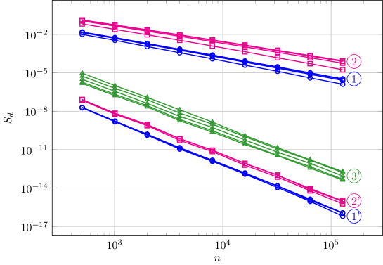
Figure 1: The values of $S_{d}({\boldsymbol{z}})$ against $n$ for different weights: (1) product – blue, (2) POD – magenta, (3) SPOD – green, with $\alpha=2$ (top two groups) and $\alpha=4$ (bottom three groups). Each group includes five lines representing $d\in\{5,10,20,50,100\}$. The empirical rates of convergence for the five groups are roughly $n^{-1.3},n^{-1.6},n^{-3.1},n^{-3.3},n^{-3.5}$ from top down.

We see from Figure 1 that the different values of target dimension $d$ do not appear to affect the empirical rates of convergence, which is consistent with our theory. For $\alpha=2$ we observe roughly the rates ${\mathcal{O}}(n^{-1.3})$ for POD weights and ${\mathcal{O}}(n^{-1.6})$ for product weights, compared with the theoretical rate of nearly ${\mathcal{O}}(n^{-2})$. For $\alpha=4$ we get roughly ${\mathcal{O}}(n^{-3.1})$ for SPOD weights, ${\mathcal{O}}(n^{-3.3})$ for POD weights, and ${\mathcal{O}}(n^{-3.5})$ for product weights, compared with the theoretical rate of nearly ${\mathcal{O}}(n^{-4})$. These empirical rates exhibit the expected trend between the cases $\alpha=2$ and $\alpha=4$.

9 Conclusion

We summarize the cost of CBC construction with different forms of weights in the theorem below.

Theorem 9.1.

The computational cost to construct a $d$-dimensional generating vector ${\boldsymbol{z}}\in\{1,\ldots,n-1\}^{d}$ for an $n$-point rank-$1$ lattice point set for approximation using the CBC construction following Algorithm 2.2 $($and satisfying Theorem 2.4 when $n$ is prime$)$ is

$${\mathcal{O}}(d\,n\log(n)+d\,n\,X)\qquad\mbox{for search and update},$$

where the values of $X$ for different forms of weights are summarized in the table below, which includes pre-computation and storage costs, and a comparison with integration.

	Integration		Approximation
Weights	$X$	Storage	$X$	Pre-comp.	Storage
product	$1$	$n$	$1$		$n$
order dep.	$d$	$d\,n$	$d\log(d)$		$d\,n$
order dep. & finite order $q$	$q$	$q\,n$	$q\log(q)$		$q\,n$
POD	$d$	$d\,n$	$d\log(d)$	$d^{2}$	$d^{2}\!+\!d\,n$
SPOD $\sigma\!\geq\!2$	$d\,\sigma^{2}$	$d\,\sigma\,n$	$d^{2}\sigma^{2}$	$d^{3}\sigma^{4}$	$d^{3}\sigma^{2}\!+\!d\,n$

In summary, the cost is ${\mathcal{O}}(d\,n\log(n))$ for product weights, ${\mathcal{O}}(d\,n\log(n)+d^{2}\log(d)\,n)$ for order dependent weights and POD weights, and ${\mathcal{O}}(d\,n\log(n)+d^{3}\sigma^{2}\,n)$ for SPOD weights with degree $\sigma\geq 2$ $($assuming $\sigma$ is small compared to $d$ and $n$$)$.

We see that the construction with SPOD weights is more costly than with POD weights. When applying a lattice algorithm in an application, it may be that the more complicated SPOD weights can lead to a better theoretical rate of convergence when we impose the requirement that the overall error bound is independent of dimension. There is then a potential trade-off between the construction cost of the lattice generating vector with these SPOD weights and the rate of convergence, which could be explored further by the users. At the same time, we can also argue that the construction of the generating vector is an offline cost and the user would be able to pick an already existing generating vector, constructed for a space with very similar SPOD weights, therefore immediately benefiting from the better convergence rate.

The best possible rate of convergence for lattice algorithms for approximation is proved [1] to be only half of the optimal rate of convergence for lattice rules for integration (i.e., ${\mathcal{O}}(n^{-\alpha/4+\delta})$ versus ${\mathcal{O}}(n^{-\alpha/2+\delta})$, $\delta>0$). This is a negative point for lattice algorithms, since there are other approximation algorithms such as Smolyak algorithms or sparse grids which do not suffer from this loss of convergence rate. However, as discussed in [1], lattice algorithms have their advantages in terms of simplicity of construction and point generation, and stability and efficiency in application, making them still attractive and competitive despite the lower convergence rate.

Instead of measuring the worst case approximation error in the $L_{2}$ norm, one can also consider other $L_{p}$ norms, including the $L_{\infty}$ norm. Also the underlying Hilbert space $H_{d}$ can be changed into a Banach space with, for example, a supremum norm. The error analysis from [4] as well as the fast algorithms from this paper can be adapted.

Also related are spline algorithms or kernel methods [52, 53, 54] or collocation [34, 49] based on lattice points. In a reproducing kernel Hilbert space with a “shift-invariant” kernel (as we have in the periodic setting here), the structure of the lattice points allows the required linear system to be solved in ${\mathcal{O}}(n\log(n))$ operations. Since splines have the smallest worst case $L_{2}$ approximation error among all algorithms that make use of the same sample points (see for example [54]), the lattice generating vectors constructed from this paper can be used in a spline algorithm and the worst case error bound from [4] will carry over as an immediate upper bound with no further multiplying constant. The advantage of a spline algorithm over the lattice algorithm (2.1) is that there is no presence of the index set ${\mathcal{A}}_{d}$, making it extremely efficient in practice.

Acknowledgements

We gratefully acknowledge the financial support from the Australian Research Council (DP180101356).

References

[1]
G. Byrenheid, L. Kämmerer, T. Ullrich, T. Volkmer,
Tight error bounds for rank- lattice sampling in spaces of hybrid mixed smoothness,
Numer. Math., 136 (2017), 993–1034.
[2]
A. Cohen, R. DeVore, Ch. Schwab,
Convergence rates of best -term Galerkin approximations
for a class of elliptic sPDEs,
Found. Comp. Math., 10 (2010), 615–646.
[3]
R. Cools, F. Y. Kuo, D. Nuyens,
Constructing embedded lattice rules for multivariate integration,
SIAM J. Sci. Comput., 28 (2006), 2162–2188.
[4]
R. Cools, F. Y. Kuo, D. Nuyens, I. H. Sloan,
Lattice algorithms for multivariate approximation in periodic spaces with general weight parameters,
to appear in: Celebrating 75 Years of Mathematics of Computation
(S. C. Brenner, I. Shparlinski, C.-W. Shu, and D. Szyld, eds.), Contemporary
Mathematics, AMS.
[5]
R. Cools, F. Y. Kuo, D. Nuyens, G. Suryanarayana,
Tent-transformed lattice rules for integration and approximation of
multivariate non-periodic functions, J. Complexity, 36 (2016), 166–181.
[6]
R. Cools, D. Nuyens,
A Belgian view on lattice rules,
in: Monte Carlo and Quasi-Monte Carlo Methods 2006
(A. Keller, S. Heinrich, and H. Niederreiter, eds.),
Springer, 2008, pp. 3–21.
[7]
J. Dick,
Walsh spaces containing smooth functions and
Quasi-Monte Carlo rules of arbitrary high order,
SIAM J. Numer. Anal., 46 (2008), 1519–1553.
[8]
J. Dick, P. Kritzer, F. Y. Kuo, I. H. Sloan,
Lattice-Nyström method for Fredholm integral equations of the second kind with convolution type kernels,
J. Complexity, 23 (2007), 752–772.
[9]
J. Dick, F. Y. Kuo, Q. T. Le Gia, D. Nuyens, Ch. Schwab,
Higher order QMC Galerkin discretization for parametric
operator equations,
SIAM J. Numer. Anal., 52 (2014), 2676–2702.
[10]
J. Dick, F. Y. Kuo, I. H. Sloan,
High-dimensional integration: the Quasi-Monte Carlo way,
Acta Numer., 22 (2013), 133–288.
[11]
J. Dick, F. Pillichshammer,
Digital Nets and Sequences,
Cambridge University Press, Cambridge, 2010.
[12]
J. Dick, I. H. Sloan, X. Wang, H. Woźniakowski,
Good lattice rules in weighted Korobov spaces with general weights,
Numer. Math., 103 (2006), 63–97.
[13]
A. Ebert, H. Leövey, D. Nuyens,
Successive coordinate search and component-by-component construction of rank- lattice rules,
in: Monte Carlo and Quasi-Monte Carlo Methods 2016 (A. B. Owen and P. W. Glynn, eds.),
Springer-Verlag, 2018, pp. 197–215.
[14]
I. G. Graham, F. Y. Kuo, J. A. Nichols, R. Scheichl, Ch. Schwab, I. H. Sloan,
Quasi-Monte Carlo finite element methods for elliptic PDEs with lognormal random coefficients,
Numer. Math., 131 (2015), 329–368.
[15]
I. G. Graham, F. Y. Kuo, D. Nuyens, R. Scheichl, and I. H. Sloan,
Circulant embedding with QMC: analysis for elliptic PDE with lognormal coefficients,
Numer. Math., 140 (2018), 479–511.
[16]
F. J. Hickernell,
Lattice rules: How well do they measure up?,
in: Random and Quasi-Random Point Sets (P. Hellekalek and G. Larcher, eds.),
Springer, Berlin, 1998, pp. 109–166.
[17]
F. J. Hickernell, H. S. Hong,
Quasi-Monte Carlo methods and their randomisations,
in: Applied Probability, AMS/IP Studies in Advanced Mathematics, vol. 26
(R. Chan, Y.-K. Kwok, D. Yao, and Q. Zhang, eds.),
American Mathematical Society, Providence, 2002, pp. 59–77.
[18]
V. Kaarnioja, F. Y. Kuo, I. H. Sloan,
Uncertainty quantification using periodic random variables,
submitted 2019.
[19]
L. Kämmerer,
Reconstructing hyperbolic cross
trigonometric polynomials from sampling along rank- lattices,
SIAM J. Numer. Anal., 51 (2013), 2773–2796.
[20]
L. Kämmerer, D. Potts, T. Volkmer,
Approximation of multivariate periodic functions by trigonometric polynomials based on rank- lattice sampling,
J. Complexity, 31 (2015), 543–576.
[21]
D. Krieg, M. Ullrich,
Function values are enough for -approximation,
arXiv:1905.02516.
[22]
F. Y. Kuo,
Component-by-component constructions achieve the optimal rate of convergence
for multivariate integration in weighted Korobov and Sobolev spaces,
J. Complexity, 19 (2003), 301–320.
[23]
F. Y. Kuo, G. Migliorati, F. Nobile, D. Nuyens,
Function integration, reconstruction and approximation using rank- lattices,
submitted 2019.
[24]
F. Y. Kuo, D. Nuyens,
Application of quasi-Monte Carlo methods to elliptic PDEs with
random diffusion coefficients – a survey of analysis and
implementation,
Found. Comput. Math., 16 (2016), 1631–1696.
[25]
F. Y. Kuo, Ch. Schwab, I. H. Sloan,
Quasi-Monte Carlo methods for high-dimensional integration: the standard (weighted Hilbert space) setting and beyond,
The ANZIAM Journal, 53 (2011), 1–37.
[26]
F. Y. Kuo, Ch. Schwab, I. H. Sloan,
Quasi-Monte Carlo finite element methods for a class of elliptic partial
differential equations with random coefficient,
SIAM J. Numer. Anal., 50 (2012), 3351–3374.
[27]
F. Y. Kuo, I. H. Sloan, G. W. Wasilkowski, H. Woźniakowski,
On decompositions of multivariate functions,
Math. Comp., 79 (2010), 953–966.
[28] F. Y. Kuo, I. H. Sloan, H. Woźniakowski,
Lattice rules for multivariate approximation in
the worst case setting, in:
Monte Carlo and Quasi-Monte Carlo Methods 2004 (H. Niederreiter and D. Talay, eds),
Springer, 2006, pp. 289–330.
[29] F. Y. Kuo, I. H. Sloan, H. Woźniakowski,
Lattice rule algorithms for multivariate approximation in the
average case setting,
J. Complexity, 24 (2008), 283–323.
[30] F. Y. Kuo, G. W. Wasilkowski, H. Woźniakowski,
On the power of standard information for multivariate approximation
in the worst case setting,
J. Approx. Theory, 158 (2009), 97–125.
[31]
P. L’Ecuyer, D. Munger,
On figures of merit for randomly shifted lattice rules,
in: Monte Carlo and Quasi-Monte Carlo Methods 2010
(L. Plaskota and H. Woźniakowski, eds.),
Springer, 2012, pp. 133–159.
[32]
C. Lemieux,
Monte Carlo and Quasi-Monte Carlo Sampling,
Springer, New York, 2009.
[33]
G. Leobacher, F. Pillichshammer,
Introduction to Quasi-Monte Carlo Integration and Applications,
Springer, 2014.
[34]
D. Li, F. J. Hickernell,
Trigonometric spectral collocation methods on lattices, in:
Recent Advances in Scientific Computing and
Partial Differential Equations (S. Y. Cheng, C.-W. Shu, and T. Tang, eds.),
AMS Series in Contemporary Mathematics, vol. 330, American
Mathematical Society, Providence, Rhode Island, 2003, pp. 121–132.
[35] H. Niederreiter,
Random Number Generation and Quasi-Monte Carlo Methods, SIAM, 1992.
[36] E. Novak, I. H. Sloan, H. Woźniakowski,
Tractability of approximation for weighted Korobov spaces on
classical and quantum computers,
Found. Comput. Math. 4 (2004), 121–156.
[37]
E. Novak, H. Woźniakowski,
Tractability of Multivariate Problems, Volume I: Linear Information,
EMS, Zürich, 2008.
[38]
E. Novak, H. Woźniakowski,
Tractability of Multivariate Problems, Volume II: Standard Information for Functionals,
EMS, Zürich, 2010.
[39]
E. Novak, H. Woźniakowski,
Tractability of Multivariate Problems, Volume III: Standard Information for Operators,
EMS, Zürich, 2012.
[40]
D. Nuyens,
The construction of good lattice rules and polynomial lattice rules,
in: Uniform Distribution and Quasi-Monte Carlo Methods
(P. Kritzer, H. Niederreiter, F. Pillichshammer, A. Winterhof, eds.),
Radon Series on Computational and Applied Mathematics Vol. 15,
De Gruyter, 2014, pp. 223–256.
[41]
D. Nuyens, R. Cools,
Fast algorithms for component-by-component construction of rank- lattice rules
in shift-invariant reproducing kernel Hilbert spaces,
Math. Comp., 75 (2006), 903–920.
[42]
D. Nuyens, R. Cools,
Fast component-by-component construction of rank- lattice rules with a non-prime number of points,
J. Complexity 22 (2006), 4–28.
[43]
D. Nuyens, R. Cools,
Fast component-by-component construction, a reprise for different kernels,
in:
Monte Carlo and quasi-Monte Carlo methods 2004
(H. Niederreiter, D. Talay, eds.),
Springer, Berlin, 2006, pp. 373–387.
[44]
D. Nuyens, G. Suryanarayana, M. Weimar,
Construction of quasi-Monte Carlo rules for multivariate integration in
spaces of permutation-invariant functions,
Construc. Approx. 45 (2017), 311–344.
[45] D. Potts, T. Volkmer,
Sparse high-dimensional FFT based on rank- lattice sampling,
Appl. Comput. Harmon. Anal., 41 (2016), 713–748.
[46]
I. H. Sloan, S. Joe,
Lattice Methods for Multiple Integration,
Oxford University Press, Oxford, 1994.
[47]
I. H. Sloan, F. Y. Kuo, and S. Joe,
Constructing randomly shifted lattice rules in weighted Sobolev
spaces,
SIAM J. Numer. Anal., 40 (2002), 1650–1665.
[48]
I. H. Sloan, A, V. Reztsov,
Component-by-component construction of good lattice rules,
Math. Comp., 71 (2002), 263–273.
[49] G. Suryanarayana, D. Nuyens, R. Cools,
Reconstruction and collocation of a class of non-periodic functions
by sampling along tent-transformed rank- lattices,
J. Fourier Anal. App., 22 (2016), 187–214.
[50]
I. H. Sloan, H. Woźniakowski,
When are quasi-Monte Carlo algorithms efficient for
high-dimensional integrals?,
J. Complexity, 14 (1998), 1–33.
[51]
I. H. Sloan, H. Woźniakowski,
Tractability of multivariate integration for weighted Korobov classes,
J. Complexity, 17 (2001), 697–721.
[52]
G. Wahba,
Spline Models for Observational Data,
SIAM, Philadelphia, 1990.
[53] X. Y. Zeng, K. T. Leung, F. J. Hickernell,
Error analysis of splines for periodic problems using lattice designs,
in:
Monte Carlo and Quasi-Monte Carlo Methods 2004 (H. Niederreiter and D. Talay, eds), Springer, 2006, pp. 501–514.
[54] X. Y. Zeng, P. Kritzer, F. J. Hickernell,
Spline methods using integration lattices and digital nets,
Constr. Approx., 30 (2009), 529–555.