Many-body localization as a $d=\infty$ Anderson localization with correlated disorder

Abstract

The disordered many-body systems can undergo a transition from the extended ensemble to a localized ensemble, known as many-body localization (MBL), which has been intensively explored in recent years. Nevertheless, the relation between Anderson localization (AL) and MBL is still elusive. Here we show that the MBL can be regarded as an infinite-dimensional AL with the correlated disorder in a virtual lattice. We demonstrate this idea using the disordered XXZ model, in which the excitation of $d$ spins over the fully polarized phase can be regarded as a single-particle model in a $d$ dimensional virtual lattice. With the increasing of $d$, the system will quickly approach the MBL phase, in which the infinite-range correlated disorder ensures the saturation of the critical disorder strength in the thermodynamic limit. From the transition from AL to MBL, the entanglement entropy and the critical exponent from energy level statics are shown to depend weakly on the dimension, indicating that belonging to the same universal class. This work clarifies the fundamental concept of MBL and presents a new picture for understanding the MBL phase in terms of AL.

Disordered many-body localized state, known as many-body localization (MBL) Basko et al. (2006); Nandkishore and Huse (2015), can be regarded as an elegant conceptual marriage of single-particle Anderson localization (AL) Anderson (1958); Fleishman and Anderson (1980); Abrahams et al. (1979) and many-body interaction. The origin of this MBL may be understood in terms of integrals of motion from the emergent integrability Huse et al. (2014), and in some particular cases can be regarded as the fixed point of some renormalization group. In experiments Bordia et al. (2017); Schreiber et al. (2015); Kohlert et al. (2019); Rispoli et al. (2019), the transition between the ergodic phase and the MBL phase and their stability are examined on various artificially engineered platforms. The long-time slow growth of entanglement entropy (EE), an important property of the MBL phase, has also been observed in recent experiments by superconducting qubits Xu et al. (2018), ultracold atoms Lukin et al. (2019) and trapped ions Brydges et al. (2019).

These two localizations possess several intimate similarities: both systems lack ergodicity Luitz and Lev (2017); Deng et al. (2017) and their energy level spacings are described by Wigner surmise in random matrix theory Mehta (2004). These features make the entropy satisfy the area law, instead of volume law Abanin et al. (2019). The MBL may be regarded as some kind of AL in the Fock space Basko et al. (2006); Bera et al. (2015), in which AL and MBL may coexist Altshuler et al. (1997); Bera et al. (2015). However, a large body of theoretical results are pointing to some multifaceted features that these two concepts are fundamentally different. For instance, MBL can be realized without single-particle AL Lev et al. (2016). While any random disorder can induce AL in one dimensional model, a finite disorder strength is required for MBL Luitz et al. (2015), which is more resemblance to three dimensional AL. It seems that the dimension is an unimportant degree of freedom in MBL since this phase can also be realized in quantum dot Altshuler et al. (1997); Gornyi et al. (2016). To date, the central concept that the relation between these two localizations is elusive and a consensus definition of MBL is still lacked.

Here we present an idea that the MBL can be regarded as an infinite-dimensional AL with the correlated disorder in a virtual lattice by the Fock states. We demonstrate this conclusion using the widely studied random XXZ model, in which the excitation of $d$ spins over the fully polarized state can be mapped to a $d$ dimensional tight-binding model with infinite-range correlated disorder. By varying $d$ from 1 to infinity, we observe a sharp transition from AL to MBL. The MBL is characterized by the energy level spacing ratio, with $W_{c}(d\rightarrow\infty)\rightarrow 3.817$ based on extrapolation to a large $d$ limit. During the crossover from AL to MBL, the critical exponent for energy level statistics is shown to dimension independent. The infinite-range correlated disorder induce the saturation of $W_{c}$ with the increasing of dimension. The dynamics of EE is shown to be a smooth crossover from AL to MBL. These features indicate that the AL and MBL belong to the same universal class. Our results establish a clear relation between AL and MBL, which has an important application in understanding the MBL phase in various models.

Figure 1: MBL as an infinite-dimensional AL in the virtual lattice. (a) New picture for MBL from the viewpoint of AL. The MBL phase studied in previous literature with $d=L/2$ spin excitation in the long-chain limit can be realized by the two steps along the horizontal and vertical arrows. (b) and (c) show the equivalent virtual lattice with $d=2$ and $3$, respectively. The arrows indicate the hopping between neighboring sites, and the light points indicate the unphysical regime. This idea can be straightforwardly generalized to any dimension with fermion and boson, and even models with $\mathbb{Z}_{2}$ symmetry sup .

MBL and the equivalent AL in the virtual lattice. In MBL, symmetry or conserved quantity is essential, which can decouple the Hamiltonian into different subspaces with MBL states to be defined therein. We consider the following widely studied disordered XXZ model Agarwal et al. (2015); Serbyn et al. (2014),

$$H=\sum_{i}J(S_{i}^{x}S_{i+1}^{x}+S_{i}^{y}S_{i+1}^{y})+J_{z}S_{i}^{z}S_{i+1}^{z}+h_{i}S_{i}^{z}.$$ (1)

We focus on $J=J_{z}=1$, and $h_{i}\in[-W,W]$ is an uniform random potential. This model has a conserved quantity $S_{\text{z}}=\sum_{i}S_{i}^{z}=-L/2+d$, where $d$ is the number of spin excitation over the fully polarized state $|\downarrow\rangle^{\otimes L}$. It can be reduced to the interacting Fermi-Hubbard model or Bose-Hubbard model under some proper transformation, in which the $S_{\text{z}}$ symmetry is turned to the conservation of the total number of particles Andraschko et al. (2014); Luitz and Lev (2017). For this reason, our picture for MBL can also be applied to the fermion and boson models. In the case of XYZ model with $\mathbb{Z}_{2}$ symmetry, which corresponds to the fermion and boson models with pairings, these subspaces characterized by $S_{\text{z}}$ are coupled. In this case, the subspace $S_{\text{z}}=0$ (or $d=L/2$) has the largest weight. Thus even in this limit, it can still be regarded as an infinite-dimensional AL. These concepts are explained in details in S3 sup , demonstrating the generality of our picture for MBL even with other symmetries or with other models.

Here we will look at this phase transition in a different way (see illustration in Fig. 1 (a)). The previous literature explores the physics along the line $d=L/2$ (thus $S_{\text{z}}=0$). This limit can also be reached in a different way using two steps (see the horizontal arrow and vertical arrow). Firstly, for fixed $d$, we can map the model to a $d$ dimensional lattice model, in which the critical disorder strength and the other quantities can be determined from the scaling of system size $L$. Then, we can explore these quantities by increasing the dimension $d$ to infinity. This two-step method enables us to study the crossover from AL to MBL, giving a new relation between them. For $d=0$, the quantum state is $|\downarrow\rangle^{\otimes L}$. For $d=1$, the wave function can be written as

$$\psi_{1}=\sum_{n=1}^{L}c_{n}S_{n}^{+}|\downarrow\rangle^{\bigotimes L}\equiv\sum_{n=1}^{L}c_{n}|\phi_{n}\rangle,$$ (2)

under periodic boundary condition $c_{n}=c_{n+L}$. It is important to notice that $\psi_{1}$ in the above equation is also the solution of the following tight-binding model,

$$H_{1}=\sum_{n=1}^{L}\frac{J}{2}(\hat{c}_{n}^{\dagger}\hat{c}_{n+1}+\text{h.c.})+\sum_{n=1}^{L}(E_{0}-J_{z}+\xi_{n})\hat{c}_{n}^{\dagger}\hat{c}_{n},$$ (3)

where $E_{0}=\frac{J_{z}}{4}L$, $\xi_{n}=h_{n}$ and $\hat{c}_{n}^{\dagger}$ $(\hat{c}_{n})$ is the creation (annihilation) operator at site $n$. Noticed that a constant potential $\eta=-\sum_{n}^{L}\frac{h_{n}}{2}$ is discarded. The physics in this model is well known that with the random disorder the extended eigenstate is strictly forbidden Anderson (1958); Evers and Mirlin (2008); Abrahams et al. (1979), thus $W_{c}=0$. The transition from localized phase to the extended phase can be realized in $d=1$ only with incommensurate potential in experiments Roati et al. (2008); Lahini et al. (2009).

Figure 2: Energy level statistics and the participation ratio of wave functions. In the upper panel, (a) - (c) show the universal scaling of $\langle r\rangle$ using Eq. 8, from which $W_{c}$ and $\nu$ are extracted. (d) show the distribution of $P_{\text{GOE}}$ and $P_{\text{PE}}$ (see Eq, 9). In the down panel, (e) - (f) show participated ratio $\langle S_{2}\rangle$ as a function of $\ln\mathcal{N}$. (g) and (h) show the fitted value of $a_{2}$ and $b_{2}$ for different $d$. All data are averaged by 500 - 6000 realizations.

This equivalent principle is quite general and can be realized even for $d>1$, in which the excitation of $d$ particles can be regarded as the hopping in the $d$ dimensional lattice with correlated disorder. To this end, let us define ${\bf n}=(n_{1},n_{2},\cdots,n_{d})$, then the state with $d$ spin excitations can be written as

$$\psi_{d}=\sum_{\textbf{n}}^{\mathcal{N}}c_{\textbf{n}}s_{n_{1}}^{+}s_{n_{2}}^{+}\cdots s_{n_{d}}^{+}|\downarrow\rangle^{\otimes L}\equiv\sum_{\textbf{n}}^{\mathcal{N}}c_{\textbf{n}}|\phi_{\textbf{n}}\rangle.$$ (4)

with the same periodic boundary conditions $c_{n_{1}n_{2}\cdots n_{d}}=c_{n_{2}n_{3}\cdots n_{d},n_{1+L}}$. One should be noticed that the number of lattice sites in the physics space is $\mathcal{N}=C_{L}^{d}$. The virtual lattice for $d=2,3$ are shown in Figs. 1 (b) and (c), respectively. Noticed that in the definition of this state, we have imposed $n_{i}\leq n_{i+1}$ for $1\leq i\leq d-1$, thus the virtual lattice is only defined in a small lattice regime. This boundary maybe important for the study of the MBL phase in a finite lattice system, while in the large $L$ limit, its role will become negligible (S3 sup ). The equivalent tight-binding model for $|\phi_{\bf n}\rangle$ is given by

$$H_{d}=\sum_{\langle\textbf{n},\textbf{n}^{\prime}\rangle}\frac{J}{2}(\hat{c}_{\textbf{n}}^{\dagger}\hat{c}_{\textbf{n}^{\prime}}+\text{h.c.})+[\xi_{\textbf{n}}-J_{z}(d-\sum_{i}\delta_{m_{i},1})]\hat{c}_{\textbf{n}}^{\dagger}\hat{c}_{\textbf{n}},$$ (5)

where hopping ($\langle\cdot\rangle$) is allowed between neighboring sites (see the red arrows in (b) and (c) of Fig. 1), $m_{i}=n_{i+1}-n_{i}$, with random potential

$$\xi_{\mathbf{n}}=\sum_{i=1}^{d}h_{n_{i}},$$ (6)

and the constant potential $E_{0}$ and $\eta$ are discarded. We see that the many-body interaction $J_{z}$ and the random potential $h_{i}$ appear in the on-site random potential in the virtual lattice. The correlation between the random potential is given by

$$\langle\xi_{\mathbf{n}}\xi_{\mathbf{n}^{\prime}}\rangle=\langle\sum_{n_{i}\neq n_{j}^{\prime}}^{d-k}h_{n_{i}}h_{n_{j}^{\prime}}\rangle+\langle\sum_{n_{i}=n_{j}^{\prime}}^{k}h_{n_{i}}^{2}\rangle=\frac{kW^{2}}{3},$$ (7)

which indicates of infinite-range correlation with $k\leq d$. We show in Ref. sup that the on-site random potential may also be realized by the random many-body interaction Lev et al. (2016); Sierant et al. (2017), in which the single-particle AL is strictly absent. Thus our model unifies the physics of random on-site potential and random interaction.

This picture yields a new definition of MBL. It can be regarded as some kind of conceptional extension of the previous model for MBL based on the Fock state in the Bethe lattice (BL) De Luca et al. (2014). In this construction, one can define $|\mathcal{G}\rangle=|N-1\rangle$ as a ground state with $N-1$ particles, then the $(2n-1)$-th generation of the Fock state can be defined as $\mathcal{Y}^{i_{1},\cdots,i_{n}}_{j_{1},\cdots,j_{n-1}}=\hat{c}_{i_{1}}^{\dagger}\cdots\hat{c}_{i_{n}}^{\dagger}\hat{c}_{j_{1}}\cdots\hat{c}_{j_{n-1}}|\mathcal{G}\rangle$ Altshuler et al. (1997); sup . These generations can form a lattice structure (see S6 sup ), which under some approximation can be simplified to the cycle-free BL. Recent investigation has revealed the intimate relation between AL in the BL with on-site random potential and MBL Saberi (2015); nevertheless, it fails to describe the relationship between the AL and MBL. In our model, the Fock state is used, however, without the need of ground state $|\mathcal{G}\rangle$; and the node is arranged in a $d$ dimensional virtual lattice, thus the crossover from AL to MBL can be realized by increasing of dimension $d$.

Phase transition and crossover from AL to MBL. To characterize the transition from the ergodic phase to the ergodic breaking phase in the $d$ dimensional virtual lattice, we use the widely explored $r$-statistics $r=\min(s_{i+1},s_{i})/\max(s_{i+1},s_{i})$, with $s_{i}=E_{i+1}-E_{i}$ ($\{E_{i}\}$ sorted in ascending order) Atas et al. (2013). In the ergodic phase by the Gaussian orthogonal ensemble (GOE), $\langle r\rangle_{\text{GOE}}=0.5307$. In contrast, in the MBL phase with Poisson ensemble (PE), $\langle r\rangle_{\text{PE}}=0.3863$. Our results for $d=3$, 6, 10 are presented in Figs. 2 (a) - (c); more details can be found in Ref. sup . In these figures, we have adopted the scaling ansatz Luitz et al. (2015)

$$\langle r\rangle=f[(W-W_{c})L^{1/\nu}].$$ (8)

With this method, we can obtain $W_{c}$ and its corresponding critical exponent $\nu$ for different dimensions. In Fig. 2 (d), these two curves collapse to the universal form in the two ensembles Atas et al. (2013)

$$P_{\text{GOE}}(r)=\frac{27(r+r^{2})}{4(1+r+r^{2})^{5/2}},\quad P_{\text{PE}}(r)=\frac{2}{(1+r)^{2}}.$$ (9)

Figure 3: Smooth crossover from AL to MBL. The relation between $1/d$ and $W_{c}$ is presented by blue squares. The dashed line is the best fitting using Eq. 10, yielding $W_{c}(\infty)=3.817$, $\alpha=-3794$ and $\beta=4.396$. Here $W_{c}$ is slightly greater than $W_{c}=3.72$ by Luitz et. al. Luitz et al. (2015) and $W_{c}=3.8$ by Macé et. al. Macé et al. (2018); Pietracaprina et al. (2018). The green circles are results from the transfer matrix (see Ref. sup ). The inset shows the corresponding critical exponents $\nu$, which are almost independent of dimension $d$.

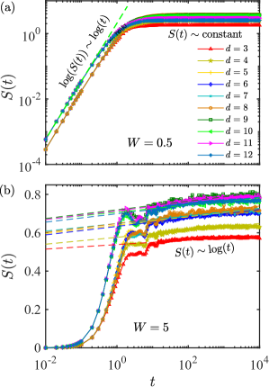
Figure 4: Information scrambling from the dynamics of half-chain EE in the crossover from AL to MBL. (a) and (b) show the scrambling of EE with $W=0.5$ (in the ergodic phase) and $W=5.0$ (in the MBL phase) as a function of $d$. For the ergodic phase we observe the power-law growth of EE $S(t)$ before saturation; while in the MBL phase, we see a logarithmic growth of $S(t)$ in the long time dynamics. All results are averaged by 2000 realizations for $L=16$.

In Fig. 3, we show the $W_{c}$ and $\nu$ for $d=3-12$; the cases for $d=1,2$ are not presented since $W_{c}=0$ sup . We find that with the increasing of $d$, $W_{c}$ will saturate to a finite value. This evolution can be described by

$$W_{c}(d)=W_{c}(\infty)+\alpha d^{-\beta}.$$ (10)

In this fitting with data for $d=6-12$ (dashed line in Fig. 3; see also S1 sup ), we obtain $\beta=4.396$ and $W_{c}(\infty)=3.817$. This critical value is slightly greater than $W_{c}=3.72$ for $L\leq 22$ in Ref. Luitz et al. (2015) and $W_{c}=3.8$ for $L\leq 24$ in Ref. Macé et al. (2018); Pietracaprina et al. (2018) coming from the finite size effect (see the open symbols based on exact diagonalization for $L\leq 14$, 16 and 18; and the scaling of $W_{c}$ as a function of $L$ in Fig. S4 sup ). This is an expected feature since in the previous literature, the choose of subspace with $S_{\text{z}}=0$ is not compulsory and in principle the same phase transition can be found for the other $S_{\text{z}}$. This is in stark contrast to the physics in AL with the uncorrelated disorder, in which $W_{c}(d)\propto d\ln d$ is expected Anderson (1958); Abrahams et al. (1979); Ueoka and Slevin (2014); García-García and Cuevas (2007). We also find that $\nu$ are almost unchanged (see inset of Fig. 3), which is also different from the previous literature that $\nu$ depends on the dimension García-García and Cuevas (2007); Tarquini et al. (2017). In our model, it is only when $d\geq 6$ that the exponent can satisfy the Harris bound. For these reasons, the infinite-range correlated disorder plays an important role in MBL and the associated saturation of $d$ in the thermodynamic limit.

One may naturally ask that why in the standard three dimensional AL, $W_{c}(3)\simeq 16.5$ and $W_{c}(d)\propto d\ln d$ in high dimensions Tarquini et al. (2017), which is much larger than $W_{c}$ in our model for MBL. In some models (such as the Aubry-André model Aubry and André (1980); Iyer et al. (2013)), the correlated disorder is expected to increase the value of $W_{c}$. To address this issue, we employ the transfer matrix to extract the value of $W_{c}$ (see S4 sup ). This method is limited by the finite size effect along the transverse direction. Our numerical results for $d=3-5$ are presented by green circles, which are significantly smaller than the value obtained from $r$-statistics. In this method, one can see that all the $L^{d-1}$ cross sections are identical, thus will not induce strong scattering between neighboring cross sections, for which reason the physics is more approaching the condition with low dimension, hence $W_{c}$ is small.

This saturation behavior may also be reflected from the wave function statistics, which are characterized by the participation entropies $S_{q}$ Luitz et al. (2015); Atas and Bogomolny (2012),

$$S_{q}=\frac{1}{1-q}\ln(\sum_{\textbf{n}}|c_{\textbf{n}}|^{2q}),$$ (11)

via $\psi_{d}=(c_{1},c_{2},c_{3},\cdots,c_{\mathcal{N}})^{T}$ in the virtual lattice. This quality characterizes the localization of the wave function in the virtual lattice with multifractal structure. In the limit $q\rightarrow 1$, this definition yields the Shannon entropy $S_{1}=-\sum_{\textbf{n}}|c_{\textbf{n}}|^{2}\ln|c_{\textbf{n}}|^{2}$; while for $q=2$, it gives $S_{2}=-\ln(\text{IPR})$, with $\text{IPR}=\sum_{\textbf{n}}|c_{\textbf{n}}|^{4}$ being the inverse participation ratio in the virtual lattice Evers and Mirlin (2008); Goltsev et al. (2012). In the ergodic ensemble, $c_{i}$ may satisfy the Gaussian distribution in the ergodic phase Casati et al. (1990): $W(c_{i})=(\mathcal{N}/2\pi)^{1/2}\exp(-\mathcal{N}c_{i}^{2}/2)$, which yields $S_{2}=\ln\mathcal{N}-1.0987$. In the fully localized phase, $c_{i}$ may be described by the Lorentz distribution sup : $W_{c}=\gamma/[\pi(c_{i}^{2}+\gamma^{2})]$, where $\gamma\sim\delta/\mathcal{N}$, and we have $S_{2}=\ln(\frac{3\pi}{2\delta})+\mathcal{O}(1/\mathcal{N})$. This Lorentz distribution is also consistent with that in the three dimensional AL model sup . Between these two regimes, $S_{2}$ can be well formulated using $S_{2}=a_{2}\ln\mathcal{N}+b_{2}$, with $0\leq a_{2}\leq 1$, thus $\delta=\frac{3\pi}{2e^{b_{2}}\mathcal{N}^{a_{2}}}$, which depends weakly on the system size. Our results for $d=3$ and $6$ are shown in Fig. 2 (e) and Fig. 2 (f). With the increasing of $d$, we find that $a_{2}$ will changes more and more slow during the transition from the ergodic phase to the MBL phase. Especially, in the MBL limit, they will approach the same limit (see (g) and (h) in Fig. 2). The saturation of $a_{2}$ and $b_{2}$ also indicate a smooth crossover from AL to MBL. This is expected since the AL will quickly the MBL phase as revealed from Eq. 10. We have also studied the multifractal structure of wave function in S3 sup , which agrees well with the physics in single-particle AL.

MBL from dynamics of EE. Finally, we explore the smooth crossover from AL to MBL from the dynamics of EE, which measures the information scrambling with quenched disorder. For two subsystems $A$ and $B$, the reduced density matrix for the state $|\psi\rangle$, is $\rho_{A}=\text{Tr}_{B}(|\psi\rangle\langle\psi|)$. Then the Von Neumann EE for this partition is given by $S=−\text{Tr}(\rho_{A}\ln\rho_{A})$ Bardarson et al. (2012). To study the dynamics of EE, we choose the Néel state as the initial state, and at time $t$, the wave function is obtained through $|\psi(t)\rangle=e^{-iHt}|\psi(0)\rangle$. In Fig. 4, we show the $\langle S(t)\rangle$ for different dimensions. In the ergodic phase (Fig. 4 (a)), we observe a power-law growth of EE in a short time, which quickly saturate; while in the MBL phase (Fig. 4 (b)), we see a clear logarithmic growth of $\langle S(t)\rangle$ in the long time limit Bardarson et al. (2012); Zhou and Luitz (2017). In Ref. Lukin et al. (2019), the long-time logarithmic growth of EE is understood in terms of configuration entropy. As compared with the weak disorder condition, the EE is significantly reduced with the strong disorder, indicating that there is no heating in the system and the memory of the initial state is preserved during the dynamics Smith et al. (2016); Lukin et al. (2019); Brydges et al. (2019); Xu et al. (2018). The small difference in EE for different $d$ indicate that the physics with different $d$ belong to the same universality, thus no phase transition has happened during their crossover.

Conclusions. In this work, we demonstrate that the MBL can be regarded as an infinite-dimensional AL in the virtual lattice with infinite-range correlated disorder. With the increasing of dimension, we find the critical disorder strength will quickly approach the MBL limit $W_{c}(\infty)=3.817$. The infinite-range correlation ensures the saturation of $W_{c}$ with the increasing of $d$. We also demonstrate the smooth crossover from AL to MBL by investigating the dynamics of half-chain EE, in which the different dimensions exhibit similar scaling of EE in the same phase. Our results provide a new definition of MBL and give a new theoretical basis for exploring the relationship between AL and MBL experimentally. These high dimension physics may be explored using quasiperiodic kicked rotor Casati et al. (1989); Lopez et al. (2012). Since AL in $d\geq 3$ is well defined Abrahams et al. (1979); Anderson (1958), we expect the phase transition from ergodic phase to the MBL phase is also well defined, nevertheless, since localization happens in the virtual lattice, the mobility edge should also be defined in this space, thus it may not be reflected from the real space particle diffusion Kohlert et al. (2019); Abanin et al. (2019).

This work is supported by the National Key Research and Development Program in China (Grants No. 2017YFA0304504 and No. 2017YFA0304103) and the National Natural Science Foundation of China (NSFC) with No. 11574294 and No. 11774328. M.G. is also supported by the National Youth Thousand Talents Program and the USTC startup funding.

XIDIAN UNIVERSITY

Appendix A S1: Critical disorder strength $W_{c}$ and the associated critical exponent $\nu$

Here we present some more data for the critical disorder strength $W_{c}$ and the associated critical exponent $\nu$ for different dimensions $d$. In Fig. S1, we show that the level spacing statistics $r$ for $d=2$, which yields $W_{c}=0$ and $v=2.15$ from the scaling ansatz (Eq. 8 in the main text). This means that in the two-dimensional system, any random disorder can lead to the fully localized state. In this case, the mean value of $r$ will not reach $\langle r\rangle_{\text{GOE}}=0.5307$. In Fig. S2, we show the distribution of $\langle r\rangle$ as a function of the disorder $W$ for dimensions $d=4$, 5, 7, 8, 9, 11. In Fig. S2 (a) - (f), we show the transition from the ergodic phase to the MBL phase, where the critical disorder strength near the crossing point is marked by gray shaded regimes. Using finite size scaling ansatz, we obtain the critical disorder strength $W_{c}$ and the associated critical exponent $\nu$, showing in Fig. S2 (g) - (l). A complete summary of these values and their variances are presented in Table S1. We find that while the critical disorder strengths depend strong on the dimension, the corresponding exponents are shown to be (almost) independent of $d$.

We can extract the critical disorder strength in the MBL phase for $d\rightarrow\infty$ using the following fitting

$$W_{c}(d)=W_{c}(\infty)+\alpha d^{-\beta},$$ (S1)

for $d=6-12$, which yields $W_{c}(\infty)=3.817$, $\alpha=-3794$ and $\beta=4.396$ (see Fig. S3). In Fig. S4 (a) - (c), we show the MBL transition along $d=L/2$ for $L\leq 14$, $L\leq 16$ and $L\leq 18$, respectively. This method has been used in the previous literature for the searching of $W_{c}$. We find that the exponent $\nu$ obtained in this way is the same as that in Fig. S2. In this fitting, we find that $W_{c}$ may depend strongly on the value of $L$. Using these three points, together with the data from Luitz et. al. Luitz et al. (2015) for $L\leq 22$ and Macé et. al. Macé et al. (2018); Pietracaprina et al. (2018) for $L\leq 24$, we can extract the critical disorder strength in the MBL phase using

$$W_{c}(L)=W_{c}^{\prime}(\infty)+\alpha^{\prime}L^{-\beta^{\prime}},$$ (S2)

from which we obtain $W_{c}^{\prime}(\infty)=3.889$, $\alpha^{\prime}=-58410$ and $\beta^{\prime}=4.167$ (see Fig. S4 (d)). The values of $\beta$ and $\beta^{\prime}$ in these two fittings are close to each other. This fitting shows clearly the existence of the saturation point with the increasing of $L$; however, notice that since these values are from different sources, the saturation point $W_{c}^{\prime}(\infty)$ from the second method is slightly different $W_{c}(\infty)$ from Eq. S1. Nevertheless, this new fitting and the associated saturation point can still provide valuable insight to confirm the existence of the saturation of $W_{c}$ when $d$ is approaching infinity, which is essential for our major conclusion of the main text.

Figure S1: Energy level statistics in two-dimension. (a) Show the data for $\langle r\rangle$ for different $L$ and (b) show their universal behavior based on Eq. 8 in the main text. We extract $W_{c}=0$ and $\nu=2.15$ by the best fitting. The dashed lines in each figure give $\langle r\rangle_{\text{GOE}}=0.5307$ and $\langle r\rangle_{\text{PE}}=0.3863$.

Figure S2: A summary of energy level statistics and their universal scaling. Here we consider $d=4,5,7,8,11$. In (a) - (f), the crossing points between different $L$ define the critical boundary between the ergodic phase and the MBL phase (see the gray shaded regimes). In (g) - (l), we show that all these data can collapse to a single curve based on a single parameter $(W-W_{c})L^{1/\nu}$. In this way, we obtain $W_{c}$ and $\nu$, which are shown explicitly in each figure.

Table S1: The critical disorder strength $W_{c}\pm\delta W$ and the critical exponent $\nu\pm\delta\nu$ for different dimensions $d$ .

$d$	3	4	5	6	7	8	9	10	11	12
$W_{c}$	0.726	1.094	1.682	2.38	3.08	3.403	3.59	3.675	3.71	3.74
$\delta W$	0.17	0.15	0.142	0.106	0.116	0.092	0.095	0.086	0.08	0.07
$\nu$	0.956	0.929	0.937	0.91	0.934	0.948	0.94	0.935	0.90	0.91
$\delta\nu$	0.04	0.049	0.044	0.042	0.046	0.045	0.038	0.048	0.041	0.037

Figure S3: Scaling of the critical disorder strength. The red cross with error bars are the critical disorder strength for different dimension $d$ from level spacing statistics. The solid line is our best fitting using Eq. S1, which yields $W_{c}(\infty)=3.817$, $\alpha=-3794$ and $\beta=4.396$. This data is re-plotted in Fig. 3 in the main text as a function of $1/d$ with the dashed line.

Figure S4: MBL transition along the line $d=L/2$. (a) - (b) show the universal scaling of $\langle r\rangle$ for different $L$ using Eq. 8 in the main text. (d) The red cross with error bars are from (a) - (c) and the filled symbols are given by Luitz et. al. for $L\leq 22$ ($W_{c}=3.72$) Luitz et al. (2015) and Macé et. al. for $L\leq 24$ ($W_{c}=3.8$) Macé et al. (2018); Pietracaprina et al. (2018). The blue solid line is the best for these five points using Eq. S2, which yields $W_{c}^{\prime}(\infty)=3.889$, $\alpha^{\prime}=-58410$ and $\beta^{\prime}=4.167$.

Appendix B S2: Analytical results for participation entropies $S_{q}$ in the weak and strong disorder limits

In the ergodic phase, $c_{i}$ in the wave function $\psi_{d}=(c_{1},\cdots,c_{\mathcal{N}})^{T}$ in GOE satisfies the Gaussian distribution (see Ref. Casati et al. (1990))

$$W_{\text{GOE}}(c_{i})=(A/\sigma\pi)^{1/2}\exp(-Ac_{i}^{2}/\sigma).$$ (S3)

In Fig. S5 (a) - (d), we present our numerical results for some of these wave function components. We see that the distribution of $c_{i}$ in the ergodic phase satisfies $W_{\text{GOE}}(c_{i})$, with $A\approx\mathcal{N}$ and $\sigma\approx 2$. However, in the MBL phase, we find the wave function components satisfy the Lorentz distribution

$$W_{\text{MBL}}(c_{i})=\frac{1}{\pi}\frac{\gamma}{x^{2}+\gamma^{2}},\quad\gamma=\frac{\delta}{\mathcal{N}},$$ (S4)

where $\delta$ depends weakly on $W$ and $\mathcal{N}$ in some way. Some examples are shown in Fig. S5 (e) - (h). Let us assume

$$S_{q}=\frac{1}{1-q}\ln(\sum_{\textbf{n}}^{\mathcal{N}}|c_{\textbf{n}}|^{2q})=\frac{1}{1-q}\ln(\left\langle\sum_{\textbf{n}}^{\mathcal{N}}|c_{\textbf{n}}|^{2q}\right\rangle\mathcal{N}),$$ (S5)

then in the ergodic phase, we have

$$\left\langle\sum_{\textbf{n}}^{\mathcal{N}}|c_{\textbf{n}}|^{2q}\right\rangle=\int_{-1}^{1}CW_{\text{GOE}}(x)x^{2q}\text{d}x=\frac{2^{q}[\Gamma(q+\frac{1}{2})+\Gamma(q+\frac{1}{2},\frac{\mathcal{N}}{2})]}{\sqrt{\pi}\mathcal{N}^{q}\text{Erf}(\sqrt{\mathcal{N}/2})},$$ (S6)

where $C=\text{Erf}(\sqrt{\mathcal{N}/2})$ is the normalized constant for $|c_{i}|\leq 1$, $\text{Erf}(x)$ is the Gauss error function, $\Gamma(\cdot)$ and $\Gamma(\cdot,\cdot)$ are the Gamma and incomplete Gamma functions, respectively. So for any positive integer $q$ and large $\mathcal{N}$, we have

$$S_{q}\simeq\ln\mathcal{N}+b_{q},\quad b_{q}=\frac{\ln[2^{q}\Gamma(q+1/2)/\sqrt{\pi}]}{1-q}.$$ (S7)

which means $a_{q}=1$. We find that Eq. S7 is consistent with the numerical results (see Fig. S6). When $q=0$, $\Gamma(1/2)=\sqrt{\pi}$, thus $b_{0}=0$, which is shown in Fig. S7 (a). In the MBL phase with the Lorentz distribution, we find

$$\left\langle\sum_{\textbf{n}}^{\mathcal{N}}|c_{\textbf{n}}|^{2q}\right\rangle=\int_{-1}^{1}DW_{\text{MBL}}(x)x^{2q}\text{d}x=\frac{{}_{2}F_{1}(1,\frac{1}{2}+q,\frac{3}{2}+q,-\frac{1}{\gamma^{2}})}{(1+2q)\gamma\arctan(\frac{1}{\gamma})},$$ (S8)

where $D=\frac{2}{\pi}\arctan(\frac{1}{\gamma})$ is the normalized constant for $|c_{i}|\leq 1$ and ${}_{2}F_{1}$ is the hypergeometric function. So, we find

$$S_{q}=\frac{1}{1-q}\ln[\frac{{}_{2}F_{1}(1,1/2+q,3/2+q,-1/\gamma^{2})\mathcal{N}}{(1+2q)\gamma\arctan(1/\gamma)}].$$ (S9)

For $q=2$ and large $\mathcal{N}$, we have

$$S_{2}=\ln(\frac{3\pi}{2\delta})+\mathcal{O}(\frac{1}{\mathcal{N}}).$$ (S10)

For $\delta\in[1,2]$, the result given by Eq. S10 is consistent with the numerical results in Fig. S6. So combined with the assumption $S_{2}=a_{2}\ln\mathcal{N}+b_{2}$, we have

$$\delta=\frac{3\pi}{2e^{b_{2}}\mathcal{N}^{a_{2}}},\quad\gamma=\frac{3\pi}{2e^{b_{2}}\mathcal{N}^{1+a_{2}}}$$ (S11)

This relation means that for $0\leq a_{2}\leq 1$, the width of the Lorentz distribution will decrease slightly faster than $1/\mathcal{N}$. These two coefficients depend strongly on the value of disorder strength (see Fig. 2 in the main text). This relation will be useful for us to understand the value of $\delta$ in Fig. S5, in which for $a_{2}=0.1938$ and $b_{2}=-0.1201$ (the data for $d=10$ and $W=5$ from Fig. 2 (g) - (h) in the main text), we have $\delta=1.097$, in consistent with our estimation $\delta\sim 0.945-1.64$. Here the tiny difference comes from the fluctuation of wave function components in the MBL phases. It is necessary to emphasize that the Gaussian distribution of $c_{i}$ in the ergodic phase and the Lorentz distribution of $c_{i}$ in the localized phase regime for the results in Fig. S5 can be well reproduced by the three dimensional Anderson localization model.

Figure S5: Statistics of wave function components. The upper panel and down panel have used $W=0.5$ and $W=5$, respectively, for $L=14$, $d=7$, thus $\mathcal{N}=3432$. In the first, second and third columns, we consider the statistics for $c_{10}$, $c_{500}$, $c_{1700}$ for eigenstate $\psi_{1400}$ to $\psi_{2000}$ (in the middle of the spectra). The last column shows the statistics for all wave function components from $c_{1}$ to $c_{3432}$. In the upper panel, the solid curve is fitted using the Gaussian distribution (Eq. S3) with width $\sigma/\mathcal{N}$, and in the down panel, it is fitted using the Lorentz distribution (Eq. S4) with the width by $\delta/\mathcal{N}$.

Figure S6: Numerical and analytical value of $S_{2}$. The symbols represent numerical results and the horizontal dashed lines are given by Eq. S7 for ergodic phase with $\sigma=1$, in which $\mathcal{N}=C_{42}^{3}$, $C_{15}^{6}$ and $C_{15}^{11}$ will give $S_{2}$ = 8.2498, 7.4196 and 6.1203, respectively; and Eq. S10 for MBL phase with $\delta=1$ (with $S_{2}=\ln(3\pi/2)$) and $\delta=2$ (with $S_{2}=\ln(3\pi/4)$).

Figure S7: Constant term $b_{q}$ in $S_{q}$ and the dimension of the system from $D_{0}$. (a) $b_{q}$ as a function of $q$ given by Eq. S7. (b) $D_{0}$ as a function of $1/L$ for $d=3-12$. In the thermodynamic limit $L\rightarrow\infty$, $D_{0}=d$ (Eq. S15), which means the negligible of boundary effect.

Appendix C S3: Multifractal of the wave function in the virtual lattice across the critical boundary and features identical to single particle AL

It has been widely explored that during the Anderson transition from the extended phase to the localized phase, the change of wave function can be reflected from its multifractal structures. In this section, we analysis the multifractal structure of $\psi_{i}$ in the virtual lattice. We can define the $q$-th moment as Vasquez et al. (2008)

$$P_{q}(L)=\sum_{i}|\psi_{i}|^{2q}\propto L^{-\tau(q)}.$$ (S12)

The mass exponent $\tau(q)$ is defined as

$$\tau(q)=-\lim_{L\rightarrow\infty}\frac{\ln\langle P_{q}(L)\rangle}{\ln L}\equiv d(q-1)+\Delta_{q}\equiv D_{q}(q-1),$$ (S13)

where $\Delta_{q}$ is the anomalous dimension with $\Delta_{0}=\Delta_{1}=0$ and $D_{q}$ is the generalized fractal dimension. The similarity dimension $D_{0}$ equals to the Euclidean dimension, given by

$$D_{0}=-\tau(0)=\frac{\ln\langle P_{0}(L)\rangle}{\ln L}=\frac{\ln\sum_{i}^{\mathcal{N}}|\psi_{i}|^{0}}{\ln L}=\frac{\ln\mathcal{N}}{\ln L}=\frac{\ln C_{L}^{d}}{\ln L}=\frac{\ln\frac{L!}{d!(L-d)!}}{\ln L}.$$ (S14)

For $L\gg d$, we find that

$$D_{0}\simeq\frac{\ln[L(L-1)\cdots(L-(d-1))]}{\ln L}\simeq\frac{\ln[L^{d}(1-\frac{d(d-1)}{2L})]}{\ln L}\simeq d.$$ (S15)

So, in the thermodynamic limit, we have $D_{0}=d$ (see S7 (b)). This is slightly different from the $d$-dimensional Anderson model with $D_{0}=\frac{\ln L^{d}}{\ln L}\equiv d$, which is independents of size $L$. This feature reflects the finite boundary in our virtual lattice (see Fig. 1 (b) and Fig. 1 (c) in the main text), in which the boundary effect is negligible when $L$ is large enough. The singularity spectrum $f(\alpha)$ and mass exponent $\tau(q)$ are related to each other via the Legendre transformation,

$$f(\alpha_{q})=\alpha_{q}q-\tau(q),\quad\alpha_{q}=\frac{d\tau(q)}{dq}$$ (S16)

Numerically, we can evaluate $f(\alpha_{q})$ and $\alpha_{q}$ by Vasquez et al. (2008)

$$\alpha_{q}=-\lim_{L\to\infty}\frac{1}{\ln L}\left\langle\sum_{k=1}^{\mathcal{N}}\delta_{k}(q,L)\ln\delta_{k}(1,L)\right\rangle,\quad f(\alpha_{q})=-\lim_{L\to\infty}\frac{1}{\ln L}\left\langle\sum_{k=1}^{\mathcal{N}}\delta_{k}(q,L)\ln\delta_{k}(q,L)\right\rangle,$$ (S17)

where $\delta_{k}(q,L)\equiv|\psi_{i}|^{2q}/P_{q}(L)$. In Fig. S8, we show the mass exponent $\tau_{q}$, generalized fractal dimension $D_{q}$ and singularity spectrum $f(\alpha_{q})$. The maximum value of $f(\alpha)/d$ is less than 1 due to the finite size effect (see Fig. S8 (d) and (h)), whereas in the AL model, this value is equal to 1. These features mean that the wave functions in the MBL phase have the same multifractal structure as that for the single-particle AL models. Noticed that in our model, the localization happens in the virtual lattice, instead of the real space.

Figure S8: Multifractal analysis of wave function and the similarity to single-particle AL. The first and second columns give $\tau_{q}$, $D_{q}$ as a function of $q$, the third column give $f(\alpha)/d$ as a function of $\alpha/d$ and the last column give $f(\alpha)/d$ as a function of $L$. The upper panel (a) - (c) give data for $L=24$ and $d=4$ ($W_{c}=1.09$) and the down panel (e) - (g) for $L=16$ and $d=6$ ($W_{c}=2.38$).

Appendix D S4: Transfer matrix methods in high dimensional AL with correlated disorder and the estimation of $W_{c}$

In the $d$-dimensional AL model, the critical disorder strength is shown to be proportional to $d$ (some more numerical results in Ref. Tarquini et al. (2017) show that $W_{c}\propto d\ln(d)$). For example, when $d=3$, $W_{c}=7.9$; when $d=4$, $W_{c}=17.0$ and when $d=5$, $W_{c}=28.4$. This critical boundary is much larger than the critical strength obtained in Fig. 3 in the main text. To understand this difference, we try to determine the $W_{c}$ using the transfer method. The drawback of this method is that it can only deal with some physics in small quantum systems. We treat the $d$ dimensional model with the correlated disorder and with the uncorrelated disorder in equal footing, so as to provide useful insight into the physics in our model.

To this end, we rewrite the Hamiltonian in the $d$-dimensional virtual lattice as

$$H_{d}=\sum_{\langle\textbf{n},\textbf{n}^{\prime}\rangle}\frac{J}{2}(\hat{c}_{\textbf{n}}^{\dagger}\hat{c}_{\textbf{n}^{\prime}}+h.c.)+\sum_{\textbf{n}}\xi_{\textbf{n}}\hat{c}_{\textbf{n}}^{\dagger}\hat{c}_{\textbf{n}},$$ (S18)

where we ignore the boundary condition, thus $n_{i}\in[1,L]$ ($i=1,\cdots,d$). For $d=1$, Eq. S18 can be rewritten as

$$H_{1}=\sum_{n}\frac{J}{2}(\hat{c}_{n}^{\dagger}\hat{c}_{n+1}+h.c.)+\sum_{n}h_{n}\hat{c}_{n}^{\dagger}\hat{c}_{n}.$$ (S19)

Then we have $c_{n+1}+c_{n-1}=\frac{2}{J}(E-h_{n})c_{n}$, where $c_{n}$ is the wave function on the $n$-th site and $E$ is the eigenvalue. This relation can be written in the transfer matrix form as Hoffmann and Schreiber (2012)

$$\left(\begin{array}[]{c}{c_{n+1}}\\ {c_{n}}\end{array}\right)=\left(\begin{array}[]{cc}{2(E-h_{n})}&{-1}\\ {1}&{0}\end{array}\right)\left(\begin{array}[]{c}{c_{n}}\\ {c_{n-1}}\end{array}\right)\equiv T_{n}\left(\begin{array}[]{c}{c_{n}}\\ {c_{n-1}}\end{array}\right),$$ (S20)

where $T_{n}$ is the transfer matrix, and we have set $J=1$. In general, the transfer matrix is given by

$$\left(\begin{array}[]{c}{\mathbf{c}_{n+1}}\\ {\mathbf{c}_{n}}\end{array}\right)=\left(\begin{array}[]{cc}{\mathcal{H}_{n}}&{-I}\\ {I}&{0}\end{array}\right)\left(\begin{array}[]{c}{\mathbf{c}_{n}}\\ {\mathbf{c}_{n-1}}\end{array}\right)\equiv T_{n}\left(\begin{array}[]{c}{\mathbf{c}_{n}}\\ {\mathbf{c}_{n-1}}\end{array}\right),$$ (S21)

where $\mathbf{c}_{n}$ is the wave function on the $n$-th cross-section (the dimension is $d-1$ with size $L^{d-1}$) and $\mathcal{H}_{n}$ is the Hamiltonian of the $n$-th cross-section. Eq. S21 may be solved recursively for arbitrary initial conditions $\mathbf{c}_{1}$ and $\mathbf{c}_{0}$, then, the wavefunction at $N+1$, $N$ are given by

$$\left(\begin{array}[]{c}{\mathbf{c}_{n+1}}\\ {\mathbf{c}_{n}}\end{array}\right)=T_{N}T_{N-1}\cdots T_{1}\left(\begin{array}[]{c}{\mathbf{c}_{1}}\\ {\mathbf{c}_{0}}\end{array}\right)$$ (S22)

The propagation of the transfer matrix is shown in Fig. S9. To get the amplitudes, we can calculate the product of the transfer matrix,

$$\mathcal{T}_{N}=\prod_{n=1}^{N}T_{n}=T_{N}\cdots T_{2}Q_{1}R_{1}=T_{N}\cdots T_{3}Q_{2}R_{2}R_{1}=Q_{N}R_{N}\cdots R_{1},$$ (S23)

where we use the QR decomposition ($T\equiv QR$). In the thermodynamic limit, we can define

$$\Lambda=\lim_{N\rightarrow\infty}\ln(\mathcal{T}_{N}^{\dagger}\mathcal{T}_{N})^{1/2N}=\lim_{N\rightarrow\infty}\ln(R_{1}^{\dagger}\cdots R_{N}^{\dagger}R_{N}\cdots R_{1})^{1/2N}=\lim_{N\rightarrow\infty}\ln(\prod_{n}^{N}R_{n}^{2})$$ (S24)

with eigenvalues $\lambda_{i}$ ($i=1,\cdots,L$), where $\lambda_{i}$ are the Lyapunov exponents. Then, the localization length $\xi$ is given by $\xi=(\min_{i=1\cdots L}{|\lambda_{i}|})^{-1}$. From the theorem of Oseledec Hoffmann and Schreiber (2012), we assume $\Lambda$ exist.

In Fig. S10 (a) - (b), we show the transfer matrix results of Anderson model

$$H_{\text{AL}}=\sum_{\langle i,j\rangle}(\hat{c}_{i}^{\dagger}\hat{c}_{j}+h.c.)+\sum_{i}\varepsilon_{i}\hat{c}_{i}^{\dagger}\hat{c}_{i},$$ (S25)

where $\varepsilon_{i}\in[-W,W]$ is the on-site random potential. The on-site correlation is $\langle\varepsilon_{i}^{2}\rangle=\frac{W^{2}}{3}$. However, the on-site correlation for Eq. S18 is given by $\langle\xi_{\textbf{n}}^{2}\rangle=\frac{dW^{2}}{3}$. For $d=3$ ($d=5$), we get $W_{c}=7.9\pm 0.45$ ($W_{c}=28.4\pm 0.45$), which is consistent with the previous literature $W_{c}\simeq 8.175$ ($W_{c}\simeq 28.75$) Tarquini et al. (2017).

In Fig. S10 (c) - (d), we show the localization length $\xi(L)/L$ as a function of $W$ for Eq. S18. The critical disorder $W_{c}\simeq 0.03$ and $W_{c}\simeq 0.28$ for $d=3$ and $d=5$. One can see that the critical disorder $W_{c}$ for the Anderson model with the correlated disorder is much smaller than the Anderson model without correlated disorder. Noticed that this value is still not converged due to the large localization length; however, its small value as compared with Fig. S10 (a) - (b), can still reflect some unique features of our idea for MBL. This result can be understood from the fact that in Fig. S9, all the cross-sections have the same energy levels, thus the disorder will not induce strong scattering between the different states in the neighboring cross-sections. For this reason, although the physics is essentially a high dimensional model, the scattering is more likely to be a low dimensional one (see Fig. S9 (b)), thus $W_{c}$ can be small.

Figure S9: Propagation of the transfer matrix. (a) Schematic diagram of the quasi-one-dimensional chain along the x-direction of cross-section $L^{d-1}$. $\mathcal{H}_{i}$ is the Hamiltonian in $i$-th cross-section. The sites at the same position in different cross-sections only differ by a global random potential. For this reason, although the model itself is $d$ dimension, its effect is more likely to be a low dimensional one. (b) Scattering between different states between neighboring cross-sections, which have identical scattering matrix when each cross-section is diagonalized.

Figure S10: Transfer matrix results for the $d$-dimensional AL without correlation (upper panel) and with correlation (down panel). Here we plot $\xi(L)/L$ as a function of the disorder $W$. (a) and (b) Anderson model in Eq. S25 for $d=3$ and $d=5$, and the critical disorder are $W_{c}=7.9\pm 0.45$ and $W_{c}=28.4\pm 0.45$ (see the red shaded regimes), respectively. These critical strengths are consistent with $W_{c}=8.175$ for $d=3$ and $W_{c}=28.75$ for $d=5$ presented in Ref. Tarquini et al. (2017) with much larger system sizes. For comparison, in (c) and (d) we present the AL with correlated disorder for Eq. S18 for $d=3$ and $d=5$, which yield $W_{c}=0.03\pm 0.01$ and $W_{c}=0.28\pm 0.08$, respectively. Discussion about this result is presented in the text.

Appendix E S5: MBL with fermion and boson models, physics with random interaction and the general picture for MBL with $\mathbb{Z}_{2}$ symmetry

This section address three fundamental issues. Firstly, how to apply our new definition of MBL to fermion and boson models; Secondly, what will happen in the presence of many-body random interaction, instead of random chemical potential; and finally, how to understand the physics with $\mathbb{Z}_{2}$ symmetry, for example in the XYZ model. We aim to show that in all these different cases, our basic idea that MBL can be regarded as an infinite-dimensional AL with infinite-range correlated disorder is always held.

E.1 A: Fermi-Hubbard model with the conserved number of particle

The same picture for fermion and boson can be realized in the following way. Let us consider the spinless Fermi-Hubbard model in the following way. For the model Oganesyan and Huse (2007),

$$H=-t\sum_{i}\hat{c}_{i}^{\dagger}\hat{c}_{i+1}+\text{H.c.}+U\hat{n}_{i}\hat{n}_{i+1}+v_{i}\hat{n}_{i},$$ (S26)

where $U$ is the interaction between the neighboring sites and $v_{i}$ is the random potential. We assume $d$ particles in this chain, thus we can define the following basis

$$|\phi_{\bf n}\rangle=|n_{1}n_{2}n_{3}\cdots n_{d}\rangle=\hat{c}_{n_{1}}^{\dagger}\hat{c}_{n_{2}}^{\dagger}\hat{c}_{n_{3}}^{\dagger}\cdots\hat{c}_{n_{d}}^{\dagger}|0\rangle,\quad 1\leq n_{i}<n_{i+1}\leq L,$$ (S27)

which means that only $n_{i}$-th site is occupied by one fermion particle. We find that this picture is the same as that for the spin model, thus is not repeated here.

In the following, we discuss how to incorporate this idea for fermions with spin degree of freedom. To this end, let us introduce the concept of flavor $s$, which accounts for the possible the spin degree of freedom. Then the model may be written as Luitz and Lev (2017)

$$H=-t\sum_{i,s,s^{\prime}}\hat{c}_{i,s}^{\dagger}\hat{c}_{i+1,s}+\text{H.c.}+U_{s,s^{\prime}}\hat{n}_{i,s}\hat{n}_{i+1,s^{\prime}}+v_{i,s}\hat{n}_{i,s},$$ (S28)

where $\hat{n}_{i,s}=\hat{c}_{i,s}^{\dagger}\hat{c}_{i,s}$. Let us consider the simplest case, as shown in Fig. S11, in which the spin degree of freedom can be denoted as some kind of flavor (spin configuration) in each site. In this case, the basis can still be defined in a similar way as Eq. S27, with

$$|\phi_{\bf n}\rangle=|n_{1s_{1}}n_{2s_{2}}n_{3s_{3}}\cdots n_{ds_{d}}\rangle=\hat{c}_{n_{1s_{1}}}^{\dagger}\hat{c}_{n_{2s_{2}}}^{\dagger}\hat{c}_{n_{3_{s}3}}^{\dagger}\cdots\hat{c}_{n_{ds_{d}}}^{\dagger}|0\rangle,$$ (S29)

where $n_{is_{i}}$ represents the creation of a fermion with spin $s_{i}$ at the $n_{i}$-th site and the boundary condition is $1\leq n_{1s_{1}}\leq n_{2s_{2}}\leq n_{3s_{3}}\leq\cdots\leq n_{ds_{d}}\leq L$ ($n_{is_{i}}=n_{js_{j}}$ only if $s_{i}\neq s_{j}$). The total number of excitation should be taken the flavor into account, thus

$$d=\sum_{i,s}\delta(n_{is}-1).$$ (S30)

Figure S11: Flavors in MBL for spinful fermions and bosons. Example for (a) 1-dimensional, (b) 2-dimensional virtual lattice. In each site, the spin degree of freedom in the Fermi-Hubbard model or Bose-Hubbard model can be regarded as some kind of flavor. In this way, each site in the $d$-dimensional virtual lattice can contain structure, which does not influence our basic picture for MBL.

E.2 B: Bose-Hubbard model with the conserved number of particle

The most widely explored 1D spinless Bose-Hubbard model can be written as Andraschko et al. (2014)

$$H=-t\sum_{i}^{L}\hat{b}_{i}^{\dagger}\hat{b}_{i+1}+H.c.+\frac{U}{2}\hat{n}_{i}(\hat{n}_{i}-1)+v_{i}\hat{n}_{i},$$ (S31)

where $\hat{n}_{i}=\hat{b}_{i}^{\dagger}\hat{b}_{i}$. Let us denote the basis in the same way as Eq. S27 with $1\leq n_{1}\leq n_{2}\leq n_{3}\leq\cdots\leq n_{d}\leq L$, where $n_{i}$ represents the creation of a boson at the $n_{i}$-th site and $d$ is the total number of particles. We see that except the boundary condition added $n_{i}=n_{j}$, all the other issues are exactly the same as that for the spin model.

However, for a spinful Bose-Hubbard

$$H=-t\sum_{i}^{L}\hat{b}_{i,s}^{\dagger}\hat{b}_{i+1,s}+H.c.+\frac{U_{i,s}}{2}\hat{n}_{i,s}(\hat{n}_{i,s}-1)+v_{i,s}\hat{n}_{i,s},$$ (S32)

where $\hat{n}_{i,s}=\hat{b}_{i,s}^{\dagger}\hat{b}_{i,s}$. Similar to the spinful fermion case, the basis can be defined in Eq. S29 and the spin degree of freedom can be denoted as some kind of flavor in each site, which shows in Fig. S11.

We can conclude that our basic picture of MBL as some kind of AL in the virtual lattice with the correlated disorder should be true even for spinful fermions and bosons.

E.3 C: Effect of random interaction and the equivalent long-range correlated random potential

Here we want to show that in the presence of random on-site many-body interaction, instead of random on-site disorder potential, will yield the same physics. To this end, we consider the XXZ model with periodic boundary condition in the following way,

$$H=\sum_{i}J(S_{i}^{x}S_{i+1}^{x}+S_{i}^{y}S_{i+1}^{y})+J_{z}^{i}S_{i}^{z}S_{i+1}^{z}+h\sum_{i}S_{i}^{z},$$ (S33)

where $J_{z}^{i}$ is some kind of random interaction between $i$-th site and $(i+1)$-th site. It is well-known that this term, after Jordan-Wigner transformation, will be reduced to the fermion model with many-body interaction. Following the main text, the wave function with $d$ spin excitation can be defined in Eq. 4. With the same method, The equivalent single particle tight-binding Hamiltonian for Eq. S33 is given by

$$H=\sum_{\langle\textbf{n},\textbf{n}^{\prime}\rangle}\frac{J}{2}(\hat{c}_{\textbf{n}}^{\dagger}\hat{c}_{\textbf{n}^{\prime}}+h.c.)+\sum_{\textbf{n}}[-\frac{h}{2}(L-2d)+\eta+\xi_{\textbf{n}}]\hat{c}_{\textbf{n}}^{\dagger}\hat{c}_{\textbf{n}},$$ (S34)

where $\eta=\sum_{i}^{L}\frac{J_{z}^{i}}{4}$ and the random potential

$$\xi_{\textbf{n}}=-\frac{1}{2}(J_{z}^{n_{1}-1}+J_{z}^{n_{d}})-\frac{1}{2}\sum_{i}^{d-1}[(1-\delta_{m_{i},1})(J_{z}^{n_{i}}+J_{z}^{n_{i+1}-1})],\qquad m_{i}=n_{i+1}-n_{i}.$$ (S35)

If we let $J_{z}^{i}\in[-W,W]$, for two sites ($\mathbf{n}\neq\mathbf{n}^{\prime}$), the correlation of the random potential is given by

$$\langle\xi_{\mathbf{n}}\xi_{\mathbf{n}^{\prime}}\rangle=\langle\frac{1}{4}\sum_{i,j}(J_{z}^{n_{i}-1}J_{z}^{n_{j}^{\prime}-1}+J_{z}^{n_{i}-1}J_{z}^{n_{j}^{\prime}}+J_{z}^{n_{i}}J_{z}^{n_{j}^{\prime}-1}+J_{z}^{n_{i}}J_{z}^{n_{j}^{\prime}})\rangle=\langle\frac{1}{4}\sum_{\mathcal{D}}^{k}(J_{z}^{n_{i}})^{2}\rangle=\frac{kW^{2}}{12},$$ (S36)

where $\mathcal{D}\equiv[(n_{i}=n_{j}^{\prime})$ or $(n_{i}=n_{j}^{\prime}-1)$ or $(n_{i}-1=n_{j}^{\prime})]$ and $k\leq d$. This means that the disordered many-body interaction also introduces long-range correlated disorder in the virtual lattice. However, these two cases have an important difference. In the model with random on-site potential, AL and MBL may co-exist; while in the case with random many-body interaction, the single-particle AL (for $d=1$) is strictly absent. This observation is suggestive that AL and MBL may be two totally different concepts, as discussed in the introduction of the main text.

E.4 D: XYZ model with $\mathbb{Z}_{2}$ symmetry

In the above discussion, $S_{\text{z}}$ in the XXZ model and the total number of particles in the fermion and boson models are conserved quantities, which divide the whole Hilbert space into different subspaces. In this case, the dimension $d$ is well defined. In the following XYZ model,

$$H=\sum_{i}J_{x}S_{i}^{x}S_{i+1}^{x}+J_{y}S_{i}^{y}S_{i+1}^{y}+J_{z}S_{i}^{z}S_{i+1}^{z}+h_{i}S_{i}^{z},$$ (S37)

the $S_{\text{z}}$ is not commuted with $H$, thus it is not a good quantum number. In this case, the good quantum number is characterized by

$$P_{\text{z}}=\prod_{i}S_{i}^{z},$$ (S38)

thus $P_{\text{z}}^{2}=1$ and $P_{\text{z}}=\pm 1$. This $\mathbb{Z}_{2}$ symmetry is reflected from the fact that $S_{i}^{z}\rightarrow S_{i}^{z}$ and $S_{i}^{x,y}\rightarrow-S_{i}^{x,y}$ for all $i$. In this case, the subspaces defined in the XXZ model can still be defined, however, they will be coupled by the XYZ model. In all these subspaces, the cases with $d\simeq L/2$ have the largest weight (noticed that from the Stirling formula, $C_{L}^{d}$ will approach a Gaussian distribution centered at $d=L/2$, with variance $\sigma^{2}=L$). For this reason, the MBL happened in this case can still be regarded as an infinity dimensional AL.

Let us briefly mention that after a Jordan-Wigner transformation, this model is reduced to the superconducting model, where $J_{z}$ is reduced to the interaction term. In this case, the above $\mathbb{Z}_{2}$ symmetry is reduced to the parity symmetry with even number of particles and odd number of particles. The similar physics happens to the boson models. For this reason, even in the case with other symmetries, the MBL phase can still be interpreted as some kind of AL in infinite-dimensional.

Appendix F S6: Different from our definition of MBL and the previous model with Fock state in the Bethe lattice

Figure S12: Fock space configuration and lattice constructed by these generations. (a) Fock states: the ground state of $N-1$ particles is defined by $|\mathcal{G}\rangle$; the 1-th, 3-th and 5-th generation are given by $\mathcal{Y}^{\alpha}$, $\mathcal{Y}^{\alpha\beta}_{\gamma}$ and $\mathcal{Y}^{\alpha\beta\nu}_{\gamma\mu}$. (b) Lattice formed by these generations due to coupling induced by the many-body interaction. In some limiting case, this complicated lattice structure can be reduced to the cycle-free Bethe lattice (see main text). (c) Effective hopping between different generations and the same generations give on-site potential. Any state from generation $2n-1$ is connected to states from $2n-5$, $2n-3$, $2n-1$, $2n+1$, or $2n+3$.

In this section, we aim to discuss the relation between our model and the previous definition of MBL in the lattice constructed by the Fock states, which in some limiting cases can be reduced to the cycle-free Bethe lattice. Our new definition of MBL can be regarded as some kind of conceptional extension of the previous model by placing the Fock space in a $d$ dimensional virtual lattice.

In the previous section, we have shown that our picture for MBL is applicable to spin, fermion and boson models. Here we consider the following many-body model, following the discussion in Ref. Altshuler et al. (1997)

$$H=\sum_{\alpha}\varepsilon_{\alpha}\hat{c}_{\alpha}^{\dagger}\hat{c}_{\alpha}+\sum_{xyzw}V_{xyzw}\hat{c}_{x}^{\dagger}\hat{c}_{y}^{\dagger}\hat{c}_{z}\hat{c}_{w}.$$ (S39)

Let $|\mathcal{G}\rangle=|N-1\rangle$ to be the ground state of $N-1$ particles, then the Fock states can be constructed using

$$\mathcal{Y}^{i_{1},i_{2},\cdots,i_{n}}_{j_{1},j_{2},\cdots,j_{n-1}}=\hat{c}_{i_{1}}^{\dagger}\hat{c}_{i_{2}}^{\dagger}\cdots\hat{c}_{i_{n}}^{\dagger}\hat{c}_{j_{1}}\hat{c}_{j_{2}}\cdots\hat{c}_{j_{n-1}}|\mathcal{G}\rangle,$$ (S40)

which represents $n$ particles and $n-1$ hole, form the $2n-1$ generation, which are shown in Fig. S12 (a). In these basis, the localization occurs in the Fock space of many-body states, rather than in the real space. Both single-particle and two-body interaction can be introduced into the on-site potential. By the two-body interaction, any state from generation $2n-1$ is connected to states from $2n-5$, $2n-3$, $2n-1$, $2n+1$, or $2n+3$, which is shown in Fig. S12 (c). The lattice in the Fock space of many-body states shows in Fig. S12 (b). However, in Ref. Altshuler et al. (1997), the coupling between the next nearest neighbors are ignored, which means that $V_{xyzw}=0$ for $x\neq y\neq z\neq w$ and any state from generation $2n-1$ is connected to states from $2n-3$, $2n-1$, or $2n+1$. In this limit this complicated lattice (see Fig. S12 (b)) can be reduced to the cycle-free Bethe lattice (BL).

We find that the above picture is different from our picture for MBL, though a similar basis is used. In the BL lattice model, the Fock space is represented by a single node characterized by different generations, while the structure of these nodes is not specified. However, in our model, it is characterized by the nodes in the $d$ dimensional lattice subjected to some proper boundary condition. We show in Fig. S7 that when $L\rightarrow\infty$, the dimension $D_{0}\rightarrow d$, thus the boundary effect may be neglected. Moreover, in our lattice model, no approximation is required, which naturally yields nearest neighboring interaction (see Fig. 1 (b) and Fig. 1 (c) in the main text), thus can be much more easily formulated during the numerical simulation. In our model, the dimension $d$ has specific physical meaning, thus from the conceptional point of view, our lattice model is much more transparent than the BL lattice based on different ”generations”. In our model, the construction of $|\mathcal{G}\rangle$ is not necessary. Since each node has definite physical meaning, this $d$-dimensional virtual lattice may also be useful to understand the evolution of entanglement entropy, which may contain the contribution from both the configurational entanglement entropy and number entanglement entropy Lukin et al. (2019). This new definition of MBL may also be useful to understand the absence of mobility edge in the experiment Kohlert et al. (2019); Abanin et al. (2019).

References

- Basko et al. (2006) Denis M Basko, Igor L Aleiner, and Boris L Altshuler, “Metal–insulator transition in a weakly interacting many-electron system with localized single-particle states,” Ann. Phys. 321, 1126–1205 (2006).
- Nandkishore and Huse (2015) Rahul Nandkishore and David A Huse, “Many-body localization and thermalization in quantum statistical mechanics,” Annu. Rev. Condens. Matter Phys. 6, 15–38 (2015).
- Anderson (1958) Philip W Anderson, “Absence of diffusion in certain random lattices,” Phys. Rev. 109, 1492 (1958).
- Fleishman and Anderson (1980) L Fleishman and PW Anderson, “Interactions and the anderson transition,” Phys. Rev. B 21, 2366 (1980).
- Abrahams et al. (1979) Elihu Abrahams, PW Anderson, DC Licciardello, and TV Ramakrishnan, “Scaling theory of localization: Absence of quantum diffusion in two dimensions,” Phys. Rev. Lett. 42, 673 (1979).
- Huse et al. (2014) David A. Huse, Rahul Nandkishore, and Vadim Oganesyan, “Phenomenology of fully many-body-localized systems,” Phys. Rev. B 90, 174202 (2014).
- Bordia et al. (2017) Pranjal Bordia, Henrik P Lüschen, Ulrich Schneider, Michael Knap, and Immanuel Bloch, “Periodically driving a many-body localized quantum system,” Nat. Phys. 13, 460 –464 (2017).
- Schreiber et al. (2015) Michael Schreiber, Sean S Hodgman, Pranjal Bordia, Henrik P Lüschen, Mark H Fischer, Ronen Vosk, Ehud Altman, Ulrich Schneider, and Immanuel Bloch, “Observation of many-body localization of interacting fermions in a quasirandom optical lattice,” Science 349, 842–845 (2015).
- Kohlert et al. (2019) Thomas Kohlert, Sebastian Scherg, Xiao Li, Henrik P Lüschen, Sankar Das Sarma, Immanuel Bloch, and Monika Aidelsburger, “Observation of many-body localization in a one-dimensional system with a single-particle mobility edge,” Phys. Rev. Lett. 122, 170403 (2019).
- Rispoli et al. (2019) Matthew Rispoli, Alexander Lukin, Robert Schittko, Sooshin Kim, M Eric Tai, Julian Léonard, and Markus Greiner, “Quantum critical behaviour at the many-body localization transition,” Nature 573, 385 – 389 (2019).
- Xu et al. (2018) Kai Xu, Jin-Jun Chen, Yu Zeng, Yu-Ran Zhang, Chao Song, Wuxin Liu, Qiujiang Guo, Pengfei Zhang, Da Xu, Hui Deng, et al., “Emulating many-body localization with a superconducting quantum processor,” Phys. Rev. Lett. 120, 050507 (2018).
- Lukin et al. (2019) Alexander Lukin, Matthew Rispoli, Robert Schittko, M Eric Tai, Adam M Kaufman, Soonwon Choi, Vedika Khemani, Julian Léonard, and Markus Greiner, “Probing entanglement in a many-body–localized system,” Science 364, 256–260 (2019).
- Brydges et al. (2019) Tiff Brydges, Andreas Elben, Petar Jurcevic, Benoît Vermersch, Christine Maier, Ben P Lanyon, Peter Zoller, Rainer Blatt, and Christian F Roos, “Probing rényi entanglement entropy via randomized measurements,” Science 364, 260–263 (2019).
- Luitz and Lev (2017) David J Luitz and Yevgeny Bar Lev, “The ergodic side of the many-body localization transition,” Ann. Phys. 529, 1600350 (2017).
- Deng et al. (2017) Dong-Ling Deng, Sriram Ganeshan, Xiaopeng Li, Ranjan Modak, Subroto Mukerjee, and JH Pixley, “Many-body localization in incommensurate models with a mobility edge,” Annalen der Physik 529, 1600399 (2017).
- Mehta (2004) Madan Lal Mehta, Random matrices, Vol. 142 (Elsevier, 2004).
- Abanin et al. (2019) Dmitry A. Abanin, Ehud Altman, Immanuel Bloch, and Maksym Serbyn, “Colloquium: Many-body localization, thermalization, and entanglement,” Rev. Mod. Phys. 91, 021001 (2019).
- Bera et al. (2015) Soumya Bera, Henning Schomerus, Fabian Heidrich-Meisner, and Jens H Bardarson, “Many-body localization characterized from a one-particle perspective,” Phys. Rev. Lett. 115, 046603 (2015).
- Altshuler et al. (1997) Boris L Altshuler, Yuval Gefen, Alex Kamenev, and Leonid S Levitov, “Quasiparticle lifetime in a finite system: A nonperturbative approach,” Phys. Rev. Lett. 78, 2803 (1997).
- Lev et al. (2016) Yevgeny Bar Lev, David R Reichman, and Yoav Sagi, “Many-body localization in system with a completely delocalized single-particle spectrum,” Phys. Rev. B 94, 201116 (2016).
- Luitz et al. (2015) David J Luitz, Nicolas Laflorencie, and Fabien Alet, “Many-body localization edge in the random-field Heisenberg chain,” Phys. Rev. B 91, 081103 (2015).
- Gornyi et al. (2016) IV Gornyi, AD Mirlin, and DG Polyakov, “Many-body delocalization transition and relaxation in a quantum dot,” Phys. Rev. B 93, 125419 (2016).
- (23) See supplementary materials for more details.
- Agarwal et al. (2015) Kartiek Agarwal, Sarang Gopalakrishnan, Michael Knap, Markus Müller, and Eugene Demler, “Anomalous diffusion and griffiths effects near the many-body localization transition,” Phys. Rev. Lett. 114, 160401 (2015).
- Serbyn et al. (2014) M Serbyn, Michael Knap, Sarang Gopalakrishnan, Z Papić, Norman Ying Yao, CR Laumann, DA Abanin, Mikhail D Lukin, and Eugene A Demler, “Interferometric probes of many-body localization,” Phys. Rev. Lett. 113, 147204 (2014).
- Andraschko et al. (2014) Felix Andraschko, Tilman Enss, and Jesko Sirker, “Purification and many-body localization in cold atomic gases,” Phys. Rev. Lett. 113, 217201 (2014).
- Evers and Mirlin (2008) Ferdinand Evers and Alexander D Mirlin, “Anderson transitions,” Rev. Mod. Phys. 80, 1355 (2008).
- Roati et al. (2008) Giacomo Roati, Chiara D’Errico, Leonardo Fallani, Marco Fattori, Chiara Fort, Matteo Zaccanti, Giovanni Modugno, Michele Modugno, and Massimo Inguscio, “Anderson localization of a non-interacting Bose–Einstein condensate,” Nature 453, 895 (2008).
- Lahini et al. (2009) Yoav Lahini, Rami Pugatch, Francesca Pozzi, Marc Sorel, Roberto Morandotti, Nir Davidson, and Yaron Silberberg, “Observation of a localization transition in quasiperiodic photonic lattices,” Phys. Rev. Lett. 103, 013901 (2009).
- Sierant et al. (2017) Piotr Sierant, Dominique Delande, and Jakub Zakrzewski, “Many-body localization due to random interactions,” Phys. Rev. A 95, 021601 (2017).
- De Luca et al. (2014) Andrea De Luca, BL Altshuler, VE Kravtsov, and A Scardicchio, “Anderson localization on the bethe lattice: Nonergodicity of extended states,” Phys. Rev. Lett. 113, 046806 (2014).
- Saberi (2015) Abbas Ali Saberi, “Recent advances in percolation theory and its applications,” Physics Reports 578, 1–32 (2015).
- Atas et al. (2013) YY Atas, E Bogomolny, O Giraud, and G Roux, “Distribution of the ratio of consecutive level spacings in random matrix ensembles,” Phys. Rev. Lett. 110, 084101 (2013).
- Macé et al. (2018) Nicolas Macé, Fabien Alet, and Nicolas Laflorencie, “Multifractal scalings across the many-body localization transition,” arXiv preprint arXiv:1812.10283 (2018).
- Pietracaprina et al. (2018) Francesca Pietracaprina, Nicolas Macé, David J Luitz, and Fabien Alet, “Shift-invert diagonalization of large many-body localizing spin chains,” SciPost Phys 5, 45 (2018).
- Ueoka and Slevin (2014) Yoshiki Ueoka and Keith Slevin, “Dimensional dependence of critical exponent of the anderson transition in the orthogonal universality class,” J. Phys. Soc. Jpn. 83, 084711 (2014).
- García-García and Cuevas (2007) Antonio M García-García and Emilio Cuevas, “Dimensional dependence of the metal-insulator transition,” Phys. Rev. B 75, 174203 (2007).
- Tarquini et al. (2017) Elena Tarquini, Giulio Biroli, and Marco Tarzia, “Critical properties of the anderson localization transition and the high-dimensional limit,” Phys. Rev. B 95, 094204 (2017).
- Aubry and André (1980) Serge Aubry and Gilles André, “Analyticity breaking and anderson localization in incommensurate lattices,” Ann. Israel Phys. Soc 3, 18 (1980).
- Iyer et al. (2013) Shankar Iyer, Vadim Oganesyan, Gil Refael, and David A Huse, “Many-body localization in a quasiperiodic system,” Phys. Rev. B 87, 134202 (2013).
- Atas and Bogomolny (2012) Yasar Yilmaz Atas and Eugene Bogomolny, “Multifractality of eigenfunctions in spin chains,” Phys. Rev. E 86, 021104 (2012).
- Goltsev et al. (2012) Alexander V Goltsev, Sergey N Dorogovtsev, Joao G Oliveira, and Jose FF Mendes, “Localization and spreading of diseases in complex networks,” Phys. Rev. Lett. 109, 128702 (2012).
- Casati et al. (1990) Giulio Casati, Luca Molinari, and Felix Izrailev, “Scaling properties of band random matrices,” Phys. Rev. Lett. 64, 1851 (1990).
- Bardarson et al. (2012) Jens H Bardarson, Frank Pollmann, and Joel E Moore, “Unbounded growth of entanglement in models of many-body localization,” Phys. Rev. Lett. 109, 017202 (2012).
- Zhou and Luitz (2017) Tianci Zhou and David J Luitz, “Operator entanglement entropy of the time evolution operator in chaotic systems,” Phys. Rev. B 95, 094206 (2017).
- Smith et al. (2016) Jacob Smith, Aaron Lee, Philip Richerme, Brian Neyenhuis, Paul W Hess, Philipp Hauke, Markus Heyl, David A Huse, and Christopher Monroe, “Many-body localization in a quantum simulator with programmable random disorder,” Nat. Phys. 12, 907 (2016).
- Casati et al. (1989) Giulio Casati, Italo Guarneri, and D. L. Shepelyansky, “Anderson transition in a one-dimensional system with three incommensurate frequencies,” Phys. Rev. Lett. 62, 345–348 (1989).
- Lopez et al. (2012) Matthias Lopez, Jean-Fran çois Clément, Pascal Szriftgiser, Jean Claude Garreau, and Dominique Delande, “Experimental test of universality of the anderson transition,” Phys. Rev. Lett. 108, 095701 (2012).
- Vasquez et al. (2008) Louella J Vasquez, Alberto Rodriguez, and Rudolf A Römer, “Multifractal analysis of the metal-insulator transition in the three-dimensional anderson model. I. symmetry relation under typical averaging,” Phys. Rev. B 78, 195106 (2008).
- Hoffmann and Schreiber (2012) Karl H Hoffmann and Michael Schreiber, Computational Physics: Selected Methods Simple Exercises Serious Applications (Springer, 2012).
- Oganesyan and Huse (2007) Vadim Oganesyan and David A Huse, “Localization of interacting fermions at high temperature,” Phys. Rev. B 75, 155111 (2007).