New predictions for radiation-driven, steady-state mass-loss and wind-momentum from hot, massive stars

Abstract

Context. Radiation-driven mass loss plays a key role in the life-cycles of massive stars. However, basic predictions of such mass loss still suffer from significant quantitative uncertainties.

Aims. We develop new radiation-driven, steady-state wind models for massive stars with hot surfaces, suitable for quantitative predictions of global parameters like mass-loss and wind-momentum rates.

Methods. The simulations presented here are based on a self-consistent, iterative grid-solution to the spherically symmetric, steady-state equation of motion, using full NLTE radiative transfer solutions in the co-moving frame to derive the radiative acceleration. We do not rely on any distribution functions or parametrization for computation of the line force responsible for the wind driving. The models start deep in the subsonic and optically thick atmosphere and extend up to a large radius at which the terminal wind speed has been reached.

Results. In this first paper, we present models representing two prototypical O-stars in the Galaxy, one with a higher stellar mass $M_{\ast}/M_{\odot}=59$ and luminosity $\log_{10}L_{\ast}/L_{\odot}=5.87$ (spectroscopically an early O supergiant) and one with a lower $M_{\ast}/M_{\odot}=27$ and $\log_{10}L_{\ast}/L_{\odot}=5.1$ (a late O dwarf). For these simulations, basic predictions for global mass-loss rates, velocity laws, and wind momentum are given, and the influence from additional parameters like wind clumping and microturbulent speeds discussed. A key result is that although our mass-loss rates agree rather well with alternative models using co-moving frame radiative transfer, they are significantly lower than those predicted by the mass-loss recipes normally included in models of massive-star evolution.

Conclusions. Our results support previous suggestions that Galactic O-star mass-loss rates may be overestimated in present-day stellar evolution models, and that new rates thus might be needed. Indeed, future papers in this series will incorporate our new models into such simulations of stellar evolution, extending the very first simulations presented here toward larger grids covering a range of metallicities, B supergiants across the bistability jump, and possibly also Wolf-Rayet stars.

1 Introduction

For hot, massive stars of spectral types OB, scattering and absorption in spectral lines transfer momentum from the star’s intense radiation field to the plasma, and so provides the force necessary to overcome gravity and drive a stellar wind outflow (Lucy & Solomon 1970; Castor et al. 1975; review by Puls et al. 2008). The line-driven winds of OB stars are very strong and fast, exhibiting mass-loss rates $\dot{M}\sim 10^{-5\dots-9}\,\rm M_{\odot}/yr$ and terminal wind speeds $\varv_{\infty}$ that can reach several thousand km/s. And since the radiation acceleration $g_{\rm rad}$ driving these outflows is dominated by lines from metal ions like Fe, C, N, O, etc., the winds are predicted, and shown, to depend significantly on stellar metallicity $Z_{\star}$ (e.g., Kudritzki et al., 1987; Vink et al., 2001; Mokiem et al., 2007).

The first quantitative description of such line-driven winds was given in the seminal paper by Castor et al. (1975), ”CAK”. By using the so-called Sobolev approximation in combination with an assumed power-law distribution of spectral line-strengths, CAK estimated the total line force, derived a parameterization for $g_{\rm rad}$, and developed a wind-theory that provided very useful scaling relations of $\dot{M}$ and $\varv_{\infty}$ with fundamental parameters like stellar luminosity $L_{\star}$ and mass $M_{\star}$.

Extensions of this elegant theory (Pauldrach et al., 1986; Friend & Abbott, 1986) have had considerable success in explaining many basic features of stellar winds from OB-stars. However, over the past years evidence has accumulated that such models may not be able to make quantitative predictions with the required accuracy. Namely, although CAK-type and Sobolev-based Monte-Carlo line-transfer models typically agree rather well on predicted $\dot{M}$ (Pauldrach et al., 2001; Vink et al., 2000, 2001), more recent simulations based on line radiation transfer performed in the co-moving frame (CMF), or by means of a non-Sobolev Monte-Carlo line force, seem to suggest overall lower rates (Lucy, 2007, 2010; Krtička & Kubát, 2010, 2017; Sander et al., 2017). Moreover, although the studies above, as well as this paper, focus solely on the global, steady-state wind, some time-dependent models with $g_{\rm rad}$ computed in the observer’s frame also indicate similar mass loss reductions as compared to CAK-based simulations (Owocki & Puls, 1999).

Concerning attempts to derive $\dot{M}$ directly from observations of stellar spectra, a multitude of results is scattered throughout the literature. A key uncertainty regards the effects of a clumped wind, which if neglected in the analysis may lead to rates that differ by large factors for the same star, depending on which spectral diagnostic is used to estimate $\dot{M}$ (Fullerton et al., 2006). When accounting properly for such ”wind clumping”, including the light-leakage effects of porosity in physical and velocity space, a few first multiwavelength studies of Galactic O-stars (Sundqvist et al., 2011; Šurlan et al., 2013; Shenar et al., 2015) suggest mass-loss rates that are lower than or approximately equal to those predicted by the Vink et al. (2000) standard mass-loss recipe. These results also agree well with X-ray (Cohen et al., 2014) and infra-red (Najarro et al., 2011) studies, as well as with the analysis by Puls et al. (2006) that derived upper limits on $\dot{M}$ by considering diagnostics ranging from the optical to radio. On the other hand, some extragalactic studies (Ramírez-Agudelo et al., 2017; Massa et al., 2017) find upper $\dot{M}$ limits that typically are higher than the Vink et al. recipe. Clearly, more effort will be needed here in order to place better observational constraints on the mass-loss rates from hot, massive stars.

Reduced mass-loss rates could further have quite dramatic consequences for model predictions of stellar evolution and feedback (e.g., Smith, 2014; Keszthelyi et al., 2017). Indeed, the presence of mass loss has a deciding impact on the lives and deaths of massive stars, affecting their luminosities, chemical surface abundances, rotational velocities, and nuclear burning life-times, as well as ultimately determining which type of supernova the star explodes as and which type of remnant it leaves behind (Meynet et al., 1994; Langer, 2012; Smith, 2014). As such, a key aim of this series of papers is – in addition to providing new quantitative predictions of mass loss – to incorporate our new models directly into simulations of massive-star evolution.

In this first paper, we outline the basic methods of our new wind simulations, computed using steady-state hydrodynamics and NLTE CMF radiative transfer calculations within the computer-code network fastwind (Santolaya-Rey et al., 1997; Puls et al., 2005; Carneiro et al., 2016; Puls, 2017; Sundqvist & Puls, 2018). Moreover, we present and discuss some first results from two selected models of O-stars in the Galaxy. The second paper will present results from a larger grid of such O-star simulations, covering metallicities of the Galaxy and the Magellanic Clouds (Björklund et al., in prep.). The third paper will then extend these calculations to B-stars, examining in particular mass-loss and wind-momentum properties over the so-called ”bi-stability jump” (where iron recombines from being three to two times ionized, thus providing much more driving lines, Pauldrach & Puls 1990; Vink et al. 2000). In a fourth paper we will incorporate fully our predictions into models of stellar evolution, and carefully investigate the corresponding effects (Björklund et al., in prep.). Further follow-up studies will then focus on, e.g., time-dependent effects and wind-clumping (see also $\S$4.3) and potentially even an extension of our current models to the highly evolved, classical Wolf-Rayet stars whose supersonic winds are optically thick also for optical continuum light.

2 Basic equations and assumptions

Global models (containing both the subsonic stellar photosphere and the supersonic wind outflow) are computed by a numerical, iterative grid-solution to the steady-state (time-independent) radiation-hydrodynamical conservation equations of mass and momentum in spherical symmetry. These are supplemented by considering also the energy balance, either by a method based on flux-conservation and the thermal balance of electrons (Puls et al., 2005) or by a simplified temperature structure derived from flux-weighted mean opacities in a spherical, diluted envelope (Lucy, 1971).

For gravitational acceleration $g(r)$ and (isothermal) sound speed

$$a^{2}(r)=\frac{k_{\rm b}T(r)}{\mu(r)m_{\rm h}},$$ (1)

where $T(r)$ is the temperature, $\mu(r)$ the mean molecular weight, $k_{\rm b}$ Bolzmann’s constant, and $m_{\rm h}$ the hydrogen atom mass, the equation of motion (e.o.m.) for radial velocity $\varv(r)$ is

$$\varv(r)\frac{d\varv}{dr}(r)\left(1-\frac{a^{2}(r)}{\varv(r)^{2}}\right)=g_{\rm rad}(r)-g(r)+\frac{2a^{2}(r)}{r}-\frac{da^{2}}{dr}(r).$$ (2)

The radiative acceleration

$$g_{\rm rad}(r)=\frac{\kappa_{\rm F}(r)F(r)}{c}=\frac{\kappa_{\rm F}(r)L_{\ast}}{4\pi r^{2}c},$$ (3)

where stellar luminosity $L_{\ast}$ is a fundamental input parameter of the model, $c$ is the speed of light, and the flux-weighted mean opacity $\kappa_{F}$ ($\rm cm^{2}/g$):

$$\kappa_{\rm F}F=\int\kappa_{\nu}F_{\nu}d\nu.$$ (4)

Here opacities $\kappa_{\nu}$ and radiative fluxes $F_{\nu}$ are evaluated in the frame co-moving with the fluid (the co-moving frame, CMF); to order $\varv/c$, this CMF-evaluated $g_{\rm rad}$ can then be used directly in the inertial frame e.o.m. eqn. 2 (e.g., Mihalas 1978, their eqns. 15.102-15.113). The gravity

$$g(r)=GM_{\ast}/r^{2},$$ (5)

with gravitation constant $G$, is computed from the second fundamental input parameter stellar mass $M_{\ast}$. The necessary scaling radius for setting up the adaptive radial mesh is obtained as described below, giving a ”stellar radius”

$$R_{\ast}\equiv r(\tilde{\tau}_{F}=2/3)$$ (6)

for the spherically modified flux-weighted optical depth

$$\tilde{\tau}_{F}(r)=\int\rho(r)\kappa_{F}(r)\left(\frac{R_{\ast}}{r}\right)^{2}dr.$$ (7)

The stellar ”effective temperature” is then here defined as

$$\sigma T_{\rm eff}^{4}\equiv\frac{L_{\ast}}{4\pi R_{\ast}^{2}},$$ (8)

for the Stefan-Boltzmann constant $\sigma$. Note that this differs, for example, from the models by Sander et al. (2017), where the stellar radius and effective temperature are defined at a Rosseland (rather than flux-weighted) optical depth $\tau_{\rm Ross}=20$.

Finally, mass-conservation provides the density structure for a steady-state mass-loss rate $\dot{M}$,

$$\rho(r)=\frac{\dot{M}}{4\pi r^{2}\varv(r)}.$$ (9)

For a given (also prescribed) chemical composition and metallicity $Z_{\ast}$, $g_{\rm rad}(r)$ and $a(r)$ are derived from the density, velocity, and temperature structure by using our radiative transfer and model atmosphere computer-code package fastwind (Santolaya-Rey et al., 1997; Puls et al., 2005; Carneiro et al., 2016; Puls, 2017; Sundqvist & Puls, 2018); fastwind solves for the population number-density rate equations in statistical equilibrium (typically just called NLTE) within the spherically symmetric, extended envelope (containing both the subsonic stellar photosphere and the supersonic wind outflow), including the effects from millions of metal spectral lines on the radiation field. In the version of fastwind used here, chemical abundances are scaled to the solar values by Asplund et al. (2009) and a standard helium number abundance $Y_{\rm He}=n_{\rm He}/n_{\rm H}=0.1$, $T(r)$ is derived either as before (from a flux-correction method in the lower atmosphere and the thermal balance of electrons in the outer, Puls et al. 2005), or by the simplified approach described in the next section. Most importantly, the radiation field – in particular the $g_{\rm rad}(r)$ term responsible for the wind driving – is now self-consistently computed from full solutions of the radiative transfer equations in the CMF for all included chemical elements and contributing lines (Puls, 2017); the resulting $g_{\rm rad}$ is then obtained by direct integrations of the CMF frequency-dependent fluxes and opacities.

3 Numerical calculation methods

Each model starts either from the structure obtained in a previous calculation or from a structure as computed in previous versions of fastwind (see §2 in Santolaya-Rey et al., 1997). Regarding the latter (standard) option, the key point is that there a quasi-hydrostatic atmosphere below a transition velocity $\varv\approx 0.1a(T_{\rm eff})$ is smoothly combined with an analytic ”$\beta$” wind velocity law $\varv(r)=\varv_{\infty}(1-bR_{\ast}/r)^{\beta}$, with $b$ a constant derived from the transition point velocity. This means that the equation of motion is generally not satisfied above $\varv\approx 0.1a$ and that $\dot{M}$, $\varv_{\infty}$, and $\beta$ are simply provided as input by the user. By contrast, the iterative method presented here computes predictive values for $\dot{M}$ and $\varv(r)$ for given fundamental parameters $L_{\ast}$, $M_{\ast}$, $R_{\ast}$, and $Z_{\ast}$.

The adaptive radial grid consists of 67 discrete points for computing the NLTE number densities and the radiative acceleration $g_{\rm rad}$. Whether or not the radial grid is updated between two successive iterations depends on the current distribution of grid points in column mass, velocity, and radius. In the low-velocity, optically thick parts of the atmosphere, the grid is adjusted according to a fixed distribution in column mass; around the sonic point and in the wind parts, the grid is adjusted according to the distribution of velocities and radial points. For the solution of the e.o.m. eqn. 2, a denser microgrid is used, by means of simple logarithmic interpolations from the coarser grid used in the NLTE network.

3.1 Velocity and density structure

For given values of $g_{\rm rad}(r)$ and $a(r)$, the ordinary differential equation (ODE) eqn. 2 is solved by a simple Runge-Kutta method to obtain $\varv(r)$ on the discrete radial mesh. Since the radiative acceleration here is an explicit function of only radius, eqn. 2 is critical at the sonic point $\varv=a$ (see discussion in $\S$5.4); the velocity gradient there is thus derived by applying l’Hospital’s rule, and the rest of the velocity structure then obtained by shooting up and down from the sonic point. The adaptive upper boundary typically lies between $r/R_{\ast}=100-140$ and the adaptive lower boundary is defined by computing down to a fixed column mass $m_{c}^{\rm tot}=-\int_{\infty}^{r_{\rm min}}\rho dr=80$. Adopting such a fixed $m_{c}^{\rm tot}$ stabilizes the iteration cycle somewhat, and is achieved here by using a linear regression to a Kramer-like parameterization for the flux-weighted opacity in the deepest quasi-static layers satisfying both $\varv\la 0.1$ km/s and $\tilde{\tau}_{F}>2/3$ (i.e., only in layers below $R_{\ast}$ and well below the critical sonic point):

$$\kappa_{F}\approx\kappa_{\rm e}\times(1+k_{a}\rho(a^{2}/10^{12})^{-k_{b}}),$$ (10)

where $a^{2}$ is in cgs-units, $\kappa_{\rm e}$ is the opacity due to Thomson scattering, and $k_{a}$ and $k_{b}$ the corresponding fit-coefficients. This is essentially the same method as in the standard version of the fastwind code (Santolaya-Rey et al., 1997), except that we here parametrize in sound speed $a$ instead of in temperature $T$. Note that although this parametrization indeed provides quite good fits for the deep layers (see Fig. 1), it is essential to point out that it can only be applied in regions with very low velocity, where the Doppler shift effect upon the opacity is negligible.

For all layers above $\varv\approx 0.1$ km/s, the $g_{\rm rad}(r)$ computed from the CMF solution to the transfer equation is used directly, and so does not explicitly depend on density, velocity, or the velocity gradient. Thus we must find another way to update the iterative mass-loss rate than, e.g., the singularity and regularity conditions applied in CAK-theory. This mass-loss rate update can be done in various ways, and to this end we have tried several options. For example, we have preserved the total column mass down to some fixed lower boundary radius between successive iterations (Pauldrach et al., 1986; Gräfener & Hamann, 2005) or, in analogy with time-dependent models of line-driven O-star winds, we have tried fixing the density at some lower boundary radius $r_{0}$ deep in the atmosphere and let the corresponding velocity $\varv_{0}$ float and iteratively adjust itself to the overlying wind conditions (e.g., Owocki et al., 1988; Sundqvist & Owocki, 2013). Just like Sander et al. (2017), however, we find that (at least among the methods tried thus far) the most stable way to update $\dot{M}$ is to instead consider the error in the force balance at the previous critical point $r_{\rm cr}(\varv=a)$ after a new $g_{\rm rad}$ has been computed for a given velocity and sound-speed structure. Defining

$$f_{\rm rc}=1-\frac{2a^{2}}{rg}+\frac{da^{2}}{dr}\frac{1}{g},$$ (11)

this factor should equal $\Gamma=g_{\rm rad}/g$ at the sonic point if the e.o.m. eqn. 2 is fulfilled. In general within the iteration cycle though, this will not be the case unless a $\delta\Gamma=f_{\rm rc}-\Gamma$ is added to the current estimate of $\Gamma$. Since it is well known (Castor et al., 1975) that for a line-driven wind $g_{\rm rad}\propto 1/\dot{M}^{\alpha}$, with $\alpha$ some power, we may thus update our mass-loss rate for iteration $i+1$ according to $\dot{M}_{i+1}=\dot{M}_{i}\,(\Gamma/f_{\rm rc})^{1/\alpha}$. Again quite analogous to Sander et al. (2017), we find that it is typically easiest for the stability of the iteration-cycle to simply assume $\alpha=1$. We stress, however, that this (of course) does not mean that really $g_{\rm rad}\propto 1/\dot{M}$, but only that this provides a good way of updating the iterative mass-loss rate towards convergence.

3.2 Temperature structure

The radially dependent sound speed is obtained from a calculation of the temperature structure (and a radially dependent mean molecular weight). As mentioned above, the temperature update can be done self-consistently by means of a flux-conservation+electron thermal balance method. In this case, the calculation is done in parallel with computing a new estimate of $g_{\rm rad}$, requiring that both temperature and radiative acceleration be converged before the next update of velocity and density. However, since converging temperature and radiative acceleration in parallel is very time-consuming, and sometimes leads to somewhat un-stable iteration cycles, most models here instead update the temperature structure using a simplified method. Namely, following Lucy (1971) we may estimate the temperature structure in the spherically extended envelope as

$$T(r)=T_{\rm eff}\left(W(r)+3\tilde{\tau}_{F}(r)/4\right)^{1/4}$$ (12)

for dilution factor $W(r)=1/2\left(1-\sqrt{1-R_{\ast}^{2}/r^{2}}\right)$ and where for radii $r<R_{\ast}$ simply $W=1/2$. Analogous to the standard version of fastwind, we also here impose a floor-temperature of typically $T\approx 0.4T_{\rm eff}$ in order to prevent excessive cooling in the outermost wind (see also Puls et al. 2005). Given current estimates for $g_{\rm rad}(r)$ and $\mu(r)$, eqn. 12 can now be formulated as an ODE for $da^{2}/dr$ and solved in parallel with the e.o.m. eqn. 2. In contrast to the flux conservation+electron thermal balance method, this temperature structure is then held fixed (along with the new $\varv(r)$ and $\rho(r)$) within the next NLTE iteration loop for obtaining the updated $g_{\rm rad}$. Although this procedure means we do not require perfect radiative equilibrium, we have found that the corresponding impact on the wind dynamics is small (see also Pauldrach et al. 1986). As such, the models in §4 all assume this structure, except for in §4.2 where a detailed comparison to a model computed from full flux-conservation+electron thermal balance is presented.

3.3 Radiative acceleration

As mentioned in the previous section, the radiative acceleration is derived from the NLTE rate equations and full solutions of the radiative transfer equation in the CMF, for all elements from H to Zn and including ”all” contributing lines (i.e. all those included in the corresponding model atoms). This is different from previous versions of fastwind, aimed at quantitive spectroscopy of optical and infra-red spectral lines, where opacities from elements not included in the detailed spectroscopic investigations (the ”background” elements) were added up to form the quasi-continuum quantities used to compute the radiation field. Although the CMF transfer solver thus is a new addition to the code (Puls, 2017), the corresponding model atoms are the same as in previous versions (coming primarily from the Munich database compiled by Pauldrach et al. 2001).

Numerous tests have been performed to verify the validity of the new CMF solver for fastwind; for example extensive comparison of ”$\beta$-law” models with the well-established cmfgen code (Hillier & Miller, 1998) shows excellent agreement between the radiative accelerations computed by the two independent programs (Puls et al., in prep., see also Fig. 1 in Puls 2017).

The radiative acceleration $g_{\rm rad}$ depends on opacities and fluxes, where the opacities are computed from a consistent NLTE solution that itself depends on the (CMF-)radiation field. After a consistent solution for the frequency-dependent opacities and fluxes have been obtained, the final $g_{\rm rad}$ is derived from direct numerical integrations. If the simplified temperature structure (see above) is applied, the procedure is performed for a given velocity, density, and temperature, and the NLTE cycle iterated until $g_{\rm rad}$ is converged. Then this $g_{\rm rad}$ is used to compute a new temperature, velocity, and density, and so forth. On the other hand, if the flux conservation+electron thermal balance method is applied, the temperature is computed in parallel with $g_{\rm rad}$, and the next hydrodynamic update of density and velocity done only when both have converged. Particularly when quite big changes between successive hydrodynamic iterations are present, this often leads to more unstable iteration-cycles and significantly slower model convergence.

Finally, just like in previous versions of fastwind (and as in basically all other 1D model atmosphere codes), we broaden all spectral line-profiles with an additional isotropic ”microturbulent” velocity $\varv_{\rm turb}$, set here to a standard O-star value 10 km/s (but see discussion in §4.4 regarding the impact of this parameter on the wind dynamics). Note that this $\varv_{\rm turb}$ also enters the calculations of the NLTE number densities and opacities, due to its influence on the radiative interaction rates.

3.4 Convergence criteria

The basic convergence criterion for our models is that the e.o.m. be fulfilled after a new $g_{\rm rad}(r)$ has been calculated from a given density and velocity structure. Re-writing the e.o.m. eqn. 2 as

$$1-\frac{\varv\frac{d\varv}{dr}\left(1-\frac{a^{2}}{\varv^{2}}\right)-g+\frac{2a^{2}}{r}-\frac{da^{2}}{dr}}{g_{\rm rad}}=f_{\rm err}$$ (13)

we note that $f_{\rm err}$ in eqn. 13 is zero in a dynamically consistent model. We thus require that

$$f_{\rm err}^{\rm max}=\rm max(\,abs(f_{\rm err})\,)$$ (14)

be below a certain threshold, typically set to $0.5-1\times 10^{-2}$ (and neglecting the deepest quasi-static layers where the Kramer-like approximation is used for $g_{\rm rad}$, see above); this means that for a converged model the e.o.m. is everywhere fulfilled to within better than a percent.

In addition, we also make sure that sufficient convergence (again typically better than a percent) is obtained for the hydrodynamic variables $\dot{M}$, $\varv$ and $T$, using the maximum relative change between two successive iterations $i-1$ and $i$. That is, for quantity X we require that

$$\rm\Delta X_{i}=max(\,abs(\,X_{i}/X_{i-1}-1\,)\,)$$ (15)

be below $\approx 0.01$.

A key point with the above is that the main convergence criterium eqn. 14 is applied directly on the actual e.o.m. Since the e.o.m. then per definition is fulfilled for a converged model, this means that we should avoid some potential difficulties related to ”false convergence”, which could (at least in principle) occur for criteria involving only relative changes between iterations of the hydrodynamic variables (such as eqn. 15). On the other hand, there is nothing in the above that guarantees that the converged solution is also unique; this is further discussed in $\S$5.4.

4 First results

Table 1: Input stellar and predicted wind parameters of models.

Model	$M_{\ast}/M_{\odot}$	$\log L_{\ast}/L_{\odot}$	$R_{\ast}/R_{\odot}$	$T_{\rm eff}$ [K]	$Z/Z_{\odot}$	$\log\dot{M}/\rm M_{\odot}/yr$	$\varv_{\infty}$ [km/s]	$\eta=\dot{M}\varv_{\infty}c/L_{\ast}$
”early” O	59.3	5.87	18.0	40 000	1.0	-5.82	2 480	0.25
”late” O	26.6	5.10	9.37	35 530	1.0	-7.59	5 300	0.05

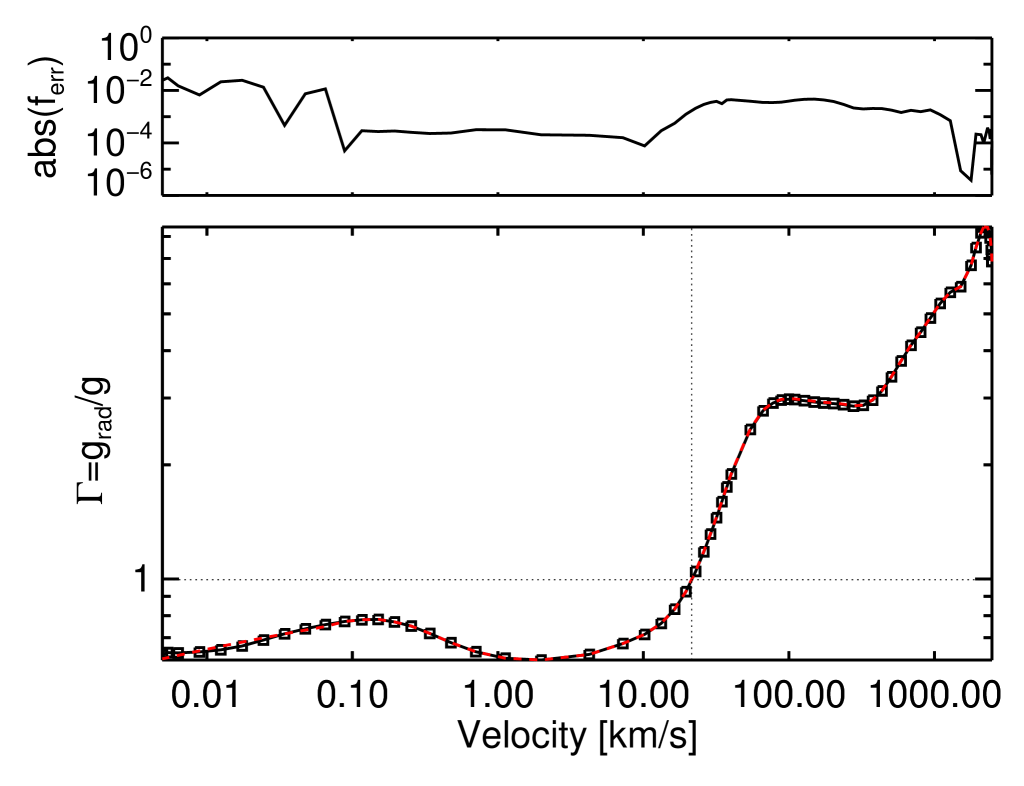
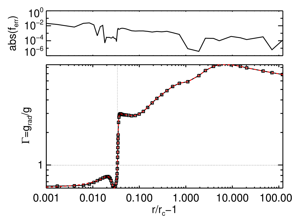
Figure 1: Final force balance for the early O-star model in Table 1. In the lower panels of both figures, the solid lines and black squares show $\Gamma=g_{\rm rad}/g$ on the discrete mesh points and the red dashed line values for the rest of the terms in the e.o.m., eqn. 2, i.e., $(1-2a^{2}/r+da^{2}/dr+\varv d\varv/dr(1-a^{2}/\varv^{2}))/g$. Since the e.o.m. is perfectly fulfilled, the solid black lines and the dashed red ones lie directly on top of each other in the figure. The dotted lines mark the sonic point $\varv=a$. The upper panels then display the absolute value of the error $f_{\rm err}$ (eqn. 13) in the e.o.m. The abscissae in the upper figure show velocity $\varv$ and in the lower scaled radius $r/r_{c}-1$, with $r_{c}$ the lower boundary radius of the simulation.

Figure 2: Upper panel: Velocity $\varv$ (solid line) and sound speed $a$ (dashed line) as function of scaled radius $r/r_{c}-1$, with $r_{c}$ the radius at the lower boundary, for the early O-star model in Table 1. The dotted lines mark the position at which $\varv=a$. Lower panel: Temperature as function of spherically modified flux-weighted optical depth $\tilde{\tau}_{F}$. The dotted lines mark the position at which $\tilde{\tau}_{F}=2/3$ (and thus $T=T_{\rm eff}$, see text).

Figure 3: Iterative evolution of quantities vs. hydrodynamic iteration number $i$. The uppermost panel shows the maximum error in the e.o.m.; the second panel the relative change in velocity; the third the relative change in temperature; the fourth the mass-loss rate; and the fifth the terminal wind speed. See text.

Figure 4: Upper panel: The triangles show maximum error in the e.o.m. and the corresponding mass-loss rate for each hydrodynamic iteration $i$. Lower panel: The relative change in radiative acceleration between two successive NLTE iterations $j-1$ and $j$. The vertical dotted lines mark NLTE iterations $j$ where hydrodynamic iteration updates $i$ are made. Both panels show results from the early O-star model in Table 1.

Figure 5: Comparison of converged temperature (upper panel) and velocity (lower panel) for early O-star models computed with a simplified temperature structure (solid lines) and a flux-conservation+electron thermal balance method (dashed lines). On the abscissae are radially modified flux-weighted optical depth.

Figure 6: Comparison of converged structures for early O-star models with no wind clumping and no X-rays (see text) (sold lines), with wind clumping but without X-rays (dashed lines), and with both wind clumping and X-rays (dashed-dotted lines). The uppermost panel shows velocity vs. scaled radius and the lower two panels $\Gamma$ vs. velocity (upper) and scaled radius (lower). A clumping factor $f_{\rm cl}=10$, starting at $\varv=0.1\varv_{\infty}$, is assumed. See text.

Figure 7: Comparison of early O-star models computed for different values of ”micro-turbulent” velocity $\varv_{\rm turb}$. The upper panel compares the computed terminal wind speeds $\varv_{\infty}$ and the lower panel the mass-loss rates $\dot{M}$. Both panels have been normalized to the results of the standard model with $\varv_{\rm turb}=10\,\rm km/s$.

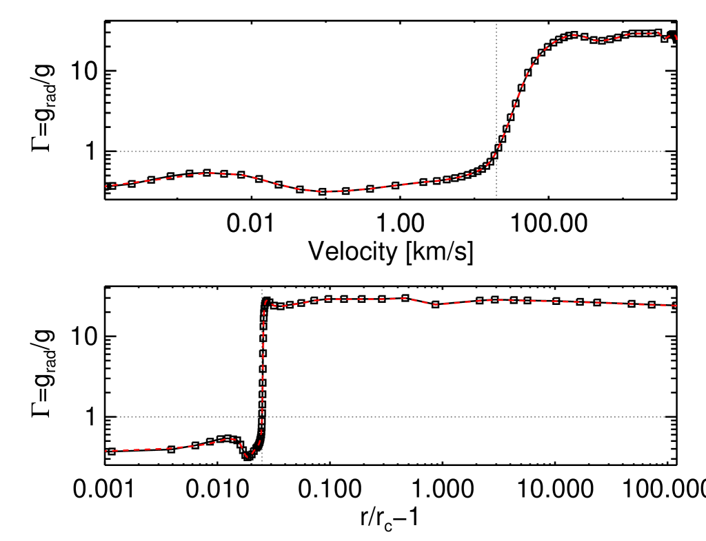
Figure 8: Final results for the ”late” O-star model, with parameters as in Table 1. The upper two panels display the $\Gamma$-factors and the lower two panels the velocity and temperature structures, analogous, respectively, to Figs. 1 and 2 for the ”early” O-star model.

Figure 9: The triangles show maximum error in the e.o.m. and the corresponding mass-loss rate for each hydrodynamic iteration $i$ for the ”late” O-star in Table 1.

Figure 10: Comparison of the velocity fields in the self-consistent hydrodynamic simulations (solid lines) to fits assuming ”single” (dashed lines) and ”double” (dashed-dotted lines) $\beta$-laws. See text. The dotted background lines compare the fits to simple $\beta=0.5$ and $\beta=1.0$ laws. The upper and lower panels show the late and early O-star models from Table 1, respectively.

Figure 11: Effective $Q_{\rm eff}$ values (eqn. 22) for the converged early O-star model (Table 1) and $\alpha=2/3$, as function of velocity (upper panel) and dimensionless radius parameter $X$ (lower panel).

Table 1 displays fundamental stellar parameters and the final predicted values for $\dot{M}$ and terminal wind speed $\varv_{\infty}$ (defined here simply as the velocity at the outermost grid-point) for two models, representing a prototypical higher-mass and lower-mass O-star in the Galaxy; following the calibration by Martins et al. (2005) the two models would be classified as an O4I and O7V star, respectively. This section presents results from these two base models, starting with a detailed analysis of the former.

4.1 Early O-star model

For the more luminous, higher-mass model, $M\approx 60M_{\odot}$, Fig. 1 displays the final, converged force balance of the simulation, demonstrating a perfect agreement between left and right hand sides in the e.o.m eqn. 2. We note further that, actually, even the lowermost part where the Kramer-like approximation (see above) is applied gives a force balance accurate to within a few percent (see upper panel) for the final fit-parameters $k_{a}=10^{13.19}$ and $k_{b}=4.611$.

The predicted mass-loss rate of the model is $1.51\times 10^{-6}\rm\,M_{\odot}/yr$, the terminal wind speed is 2480 km/s, and the scaled wind-momentum rate $\eta=\dot{M}\varv_{\infty}c/L_{\ast}=0.25$. Above the quasi-static deep layers the velocity field (illustrated in Fig. 2) displays a very steep acceleration around the sonic point, followed by a region of slower acceleration around $\sim 100$ km/s. Due to the (here implicit) dependence of $g_{\rm rad}$ on the velocity gradient in these highly supersonic regions, this feature also causes the corresponding radiative acceleration plateau visible in Fig. 1 around $\sim 100$ km/s. The radially modified flux-weighted optical depth at the sonic point is $\tilde{\tau}_{F}\approx 0.14$ and the stellar radius (per definition at $\tilde{\tau}_{F}=2/3$) is located at a velocity $\varv\approx 0.2$ km/s, i.e. well below the sonic point. We further also note the dip in radiative acceleration in the atmospheric regions leading up to the sonic point (see Fig. 1). This is qualitatively similar to the behavior observed in some earlier non-Sobolev simulations based on simplified methods to compute $g_{\rm rad}$ (Owocki & Puls 1999), however further studies are required to determine more quantitatively potential connections to those models. Fig. 2 displays the accompanying temperature structure, confirming that $T(\tilde{\tau}_{F}=2/3)=T_{\rm eff}$ but also illustrating that, of course, no temperature reversal (see §4.2) is seen in this model computed by means of the simplified eqn. 12.

Fig. 3 displays some characteristics of the iteration cycle towards hydrodynamic convergence. The top panel shows the maximum error in the e.o.m., $f_{\rm err}^{\rm max}$ (eqn. 14), the second and third panels the maximum relative change in velocity and temperature between two iterations (eqn. 15), and the two bottoms panels give the iterative evolution of mass-loss rate and terminal wind speed. The figure demonstrates how, as the error in the e.o.m. decreases, the mass-loss rate, velocity field, and temperature structure all stabilize toward convergence. Fig. 4 displays the combination of $f_{\rm err}^{\rm max}$ and $\dot{M}$ for each iteration $i$, showing again how after an initial adjustment period the mass-loss rate remains fairly constant while $f_{\rm err}^{\rm max}$ decreases towards convergence. Note again that for each such hydrodynamic iteration-update $i$ the NLTE and CMF radiative transfer computations iterate toward a new converged radiative acceleration for the given $\varv(r)_{i}$, $\rho(r)_{i}$, and $T(r)_{i}$. Fig. 4 demonstrates this, showing $\Delta g_{\rm rad,j}$ over the NLTE iteration cycle $j$; in this figure, the valleys in $\Delta g_{\rm rad,j}$ correspond to the places at which $g_{\rm rad}$ has relaxed and a new update $i$ of the hydrodynamic variables is performed.

For this simulation, the calculation started from a standard fastwind model with a ”$\beta$” velocity law and consisted in total of 345 NLTE and CMF radiative transfer iterations for computing the radiative acceleration, corresponding here to 35 hydrodynamic iteration updates. The converged final model shows $\rm\log_{10}\Delta T_{i}=-4.3$, $\rm\log_{10}\Delta\varv_{i}=-2.5$, $\rm\log_{10}\Delta\varv_{\infty,i}=-3.7$, $\rm\log_{10}\Delta\dot{M}_{i}=-3.1$, and $\log_{10}f_{\rm err}^{\rm max}=-2.3$.

4.2 Influence of temperature structure

To test the influence of the simplified temperature structure eqn. 12 upon the wind dynamics, this section computes a model with identical input parameters as for the early O-star in Table 1, but now using a full flux-conservation+electron thermal balance method (see above) to derive the run of the temperature. Indeed, also this model can be brought to convergence, but only after more than twice the number of NLTE iterations and a careful set-up of the initial ”$\beta$-law” start-model. Nonetheless, this early O-star model converges to the same mass-loss rate $\dot{M}=1.5\times 10^{-6}\,\rm M_{\odot}/yr$ and terminal wind speed $\varv_{\infty}=2500\,\rm km/s$ as previously. Fig. 5 plots the temperature and velocity structures for the two converged models, demonstrating that although the temperatures as expected reveal some differences (e.g., a small reversal is now visible; see discussion in Puls et al. 2005 for more details about this feature), the resulting velocity fields are remarkably similar.

And we can also quite readily understand this result by: i) noting that although $g_{\rm rad}$ in the optically thick, quasi-static layers is strongly dependent on the local gas temperature, in the thinner supersonic regions it becomes almost independent of it, and ii) inspecting the force balance at the sonic point and beyond, which reveals that in those regions the ”Parker terms” $2a^{2}/r-da^{2}/dr$ are less than a percent of the corresponding values of $g_{\rm rad}$ (i.e., for the supersonic part the e.o.m. is completely dominated by inertia and the counteracting radiative and gravitational accelerations).

4.3 Influence of wind clumping and X-rays

All models presented here solve the e.o.m. for a steady outflow. However, linear perturbation analysis shows the observer’s frame line force is subject to a very strong instability on scales smaller than the Sobolev length (Owocki & Rybicki, 1984). Time-dependent models (Owocki et al., 1988; Feldmeier et al., 1997; Sundqvist et al., 2018) following the non-linear evolution of this line-deshadowing instability (LDI) show a characteristic two-component-like structure consisting of spatially small and dense clumps separated by large regions of very rarified material, accompanied by strong thermal shocks and a highly non-monotonic velocity field. But as shown, e.g., in Fig. 5 of Sundqvist et al. (2018), the averaged density and velocity in such models still exhibit a smooth and steady behavior. As such, for computations aiming at predictions of global quantities, such as mass-loss rates and terminal wind speeds, it may still be reasonable to solve the hydrodynamic equations in the steady limit. Nevertheless, the overdense clumps and the high-energy radiation resulting from the wind shocks may still affect the overall wind ionization balance (e.g., Bouret et al., 2005) and $g_{\rm rad}$, and so might induce feedback-effects also upon global quantities.

Here we examine such feedback effects by computing models with identical input parameters as for the early O-star in Table 1, but now including parametrized forms of such wind clumping and X-ray emissions. X-rays are incorporated according to Carneiro et al. (2016) and clumping according to Sundqvist & Puls (2018). Note though, that in this paper we restrict the analysis to clumps that are optically thin; potential dynamical effects of porosity in physical and velocity space (Muijres et al., 2011; Sundqvist et al., 2014) will be examined in a forthcoming paper. This assumption makes the basic treatment of wind clumping here very similar to that in the alternative steady models by Sander et al. (2017) (except for the radial distribution of clumping factors). For the models displayed in Fig. 6, we have assumed that clumping starts at a velocity $\varv=0.1\varv_{\infty}$ and increases linearly in velocity until $\varv=0.2\varv_{\infty}$, outside which it remains constant at a value given by a clumping factor $f_{\rm cl}=\langle\rho^{2}\rangle/\langle\rho\rangle^{2}=\rho_{\rm cl}/\langle\rho\rangle=10$, for clump density $\rho_{\rm cl}$ and mean wind density $\langle\rho\rangle=\dot{M}/(4\pi\varv r^{2})$. While both observations (Puls et al., 2006; Najarro et al., 2011) and theory (Sundqvist & Owocki, 2013) indicate that clumping may be a more complicated function of radius, such a simple clumping-law should suffice for our test-purposes here. Note further that within the approximations used in this paper, $f_{\rm cl}$ is the inverse to the fractional wind volume $f_{\rm vol}$ occupied by clumps, i.e., here $f_{\rm cl}=f_{\rm vol}^{-1}$ (but see discussion in Sundqvist & Puls 2018). X-ray emissions are assumed to start at $r\approx 1.5R_{\ast}$ and follow the basic standard prescription outlined in Carneiro et al. (2016); the model presented in Fig. 6 has a resulting X-ray luminosity $L_{\rm x}/L_{\ast}\approx 0.8\times 10^{-7}$.

The lower panel of Fig. 6 compares $\Gamma$-factors from the simulation without clumping to i) one including only clumping but no X-rays and ii) one including both clumping and X-rays. As shown in the figure, for this particular model both these effects lead to a boost of the radiative acceleration in the outer parts of the wind. In turn then, this leads to higher wind speeds as illustrated by the upper panel of Fig. 6. Due to the steep initial wind acceleration, the assumed start-velocity for clumping $\varv=0.1\varv_{\infty}$ corresponds to a rather low radii $r/R_{\ast}\approx 1.05$, implying clumping also in near-star wind regions. However, the mass-loss rates are only marginally different though, since $g_{\rm rad}$ around the critical point is barely affected by any clumping or X-ray feedback. The model including only clumping has a final $\dot{M}=1.41\times 10^{-6}\,\rm M_{\odot}/yr$ and $\varv_{\infty}=3150\,\rm km/s$ and the model including both clumping and X-ray feedback results in $\dot{M}=1.41\times 10^{-6}\,\rm M_{\odot}/yr$ and $\varv_{\infty}=3390\,\rm km/s$.

Note finally though, that future work should examine potential feedback-effects also from models that introduce clumping in even deeper and slower atmospheric layers, which may then affect also the predicted mass-loss rates.

4.4 Influence of turbulent speed

The turbulent speed $\varv_{\rm turb}$ applied in our models (see $\S$3.3) effectively broadens the line profiles and so also affects the computation of $g_{\rm rad}$. As also discussed by, e.g., Poe et al. (1990) and Lucy (2007) this can have a significant impact upon the line acceleration in the critical sonic point region. More specifically, since a line profile extends over a few thermal+turbulent velocity widths, it means that, for our standard O-star value $\varv_{\rm turb}=10$ km/s, in the region leading up to the sonic point $a\approx 20$ km/s there is not enough velocity space available to completely Doppler shift line profiles out of their own absorption shadows. This then typically leads to a reduction of the line acceleration in these regions, as compared to Sobolev calculations where it is assumed that the line profiles are always fully de-shadowed so that the corresponding (fore-aft symmetric) line resonance zones do not extend into the stellar core. In turn, the reduced $g_{\rm rad}$ may then also reduce the predicted mass-loss rate as the overlying wind adjusts to the ”choked” sub-sonic conditions.

Fig. 7 illustrates this effect, displaying results from models computed with identical parameters as the early O-star in Table 1, but with varying turbulent velocities $\varv_{\rm turb}$. The figure shows resulting mass-loss rates and terminal wind speeds, normalised to the standard model with $\varv_{\rm turb}=$ 10 km/s. The clearly visible trend in the figure confirms the above discussion; higher turbulent velocities mean lower predicted mass-loss rates. In addition, the figure shows that this then also means higher terminal wind speeds, essentially because the supersonic wind now needs to drive less mass off the stellar surface and so more easily can accelerate. Typical numbers, for this early O-star model, are a reduction in mass loss by approximately a factor of two when increasing $\varv_{\rm turb}$ from 10 to 18 km/s, accompanied by an increase in terminal wind speed by approximately 50 %.

4.5 Late O-star model

For the lower-mass model ($M\approx 27M_{\odot}$), the upper two panels of Fig. 8 show the converged force balance analogous to Fig. 1. At first glance, the lower-mass model displays similar characteristics as the higher-mass model, however closer inspection shows that the dip in $g_{\rm rad}$ in sub-sonic layers is now somewhat more prominent, and that once the Doppler-shifted line-opacity kicks in near the sonic point $g_{\rm rad}$ very quickly shoots up to values higher than 20 times the local gravity (cmp. Fig. 1 for the higher-mass model where this rise rather results in $\Gamma\approx 3$). The steep acceleration gives rise to a fast, low-density wind with a low final mass-loss rate $\dot{M}=2.55\times 10^{-8}\,\rm M_{\odot}/yr$ and high terminal wind speed $\varv_{\infty}=5320\,\rm km/s$, giving a scaled wind-momentum rate $\eta=\dot{M}\varv_{\infty}c/L_{\ast}=0.05$.

We can readily understand the character of the fast wind by considering the e.o.m. eqn. 2 in the supersonic, zero sound-speed limit:

$$\varv\frac{d\varv}{dr}=\frac{GM_{\ast}(\Gamma-1)}{r^{2}}.$$ (16)

Noting then from Fig. 8 that $\Gamma\approx Const.\approx 27$ after the initial steep rise close to the stellar surface $R_{\ast}$, eqn. 16 can be analytically integrated to

$$\varv(r)=\varv_{\rm esc}(R_{\ast})\sqrt{\Gamma-1}\left(1-\frac{R_{\ast}}{r}\right)^{1/2},$$ (17)

yielding a terminal wind speed $\varv_{\infty}=\varv(r\rightarrow\infty)\approx 5300\rm\,km/s$ for surface escape speed $\varv_{\rm esc}(R_{\ast})=\sqrt{2GM_{\ast}/R_{\ast}}=1040\,\rm km/s$. This agrees very well with the numerically computed value in Table 1. Moreover, eqn. 17 suggests that the supersonic wind here should be quite well described by a $\beta=1/2$ velocity law; this will be confirmed in $\S$5.2, where we compare our self-consistent simulations to models with such analytic $\beta$ fields.

Further for this low-density wind model, only $\tilde{\tau}_{F}\approx 0.03$ at the sonic point and the stellar surface is located at a very low $\varv\approx 5.0\times 10^{-3}\,\rm km/s$; indeed, Fig. 8 shows an overall sub-sonic region characterized by significantly lower velocities as compared to the early O-star model, reaching $\varv\approx 10^{-4}\,\rm km/s$ at the lower boundary $m_{c}^{\rm tot}=80$.

The iterative behavior of the hydrodynamic variables shows quite similar properties as for the early O-star model displayed in Fig. 3; after an initial decrease in mass loss and increase in terminal wind speed, the simulation eventually finds its way towards convergence. We note though that numerically it is somewhat more difficult to make this model convergence, for example due to the sensitivity of the e.o.m. to the very steep acceleration around the sonic point. Fig. 9 shows $\dot{M}$ and the maximum error $f_{\rm err}^{\rm max}$ in the e.o.m. for each of the hydrodynamic iteration steps, demonstrating that although the simulation indeed reaches our convergence criteria, it does fluctuate a bit also for structures quite close to this. The final model shows $\rm\log_{10}\Delta T_{i}=-4.3$, $\rm\log_{10}\Delta\varv_{i}=-2.5$, $\rm\log_{10}\Delta\varv_{\infty,i}=-2.5$, $\rm\log_{10}\Delta\dot{M}_{i}=-2.4$, and $\log_{10}f_{\rm err}^{\rm max}=-2.2$.

5 Discussion

Having presented basic results and features above, this section now compares this paper’s two core simulations to some other O-star wind models and results that appear in the literature.

5.1 Comparison to other steady-state models

As mentioned in previous sections, the models by Sander et al. (2017) are computed on similar assumptions as those adopted here (CMF radiative transfer, spherically symmetric steady-state hydrodynamics, grid-based $g_{\rm rad}$ depending explicitly only on radius). As such, we computed an additional model adopting the same stellar parameters, $T_{\rm eff}=42\,000$ K, $R_{\ast}/R_{\odot}=15.9$, $\log_{10}L/L_{\odot}=5.85$, $\varv_{\rm turb}=15$  km/s, as in Sander et al. (2017). Note, however, that, unlike Sander et al. (2017), the simulation here used a strict solar composition for the chemical abundances and also did not include clumping; nevertheless, the models are close enough to enable a quite fair and direct comparison. Indeed, our simulation converges to $\dot{M}=1.58\times 10^{-6}\,\rm M_{\odot}/yr$, $\varv_{\infty}=2700\,\rm km/s$, and $\eta=\dot{M}\varv_{\infty}c/L_{\ast}=0.3$. For the mass-loss rate this is in perfect agreement with Sander et al. (2017), who also find $\dot{M}=1.58\times 10^{-6}\,\rm M_{\odot}/yr$. On the other hand, for the terminal wind speed (and thus the wind-momentum) they find slightly lower values, $\varv_{\infty}=2000\,\rm km/s$ and $\eta=0.23$, than here. These differences may simply be an effect of the slight differences in input parameters and basic model assumptions (abundances, clumping, definition of stellar radius, see above and $\S$2). Overall the general agreement between the two independent calculations is encouraging, however future work should investigate in more detail the impact of, e.g., wind clumping upon the wind parameters predicted by these CMF calculations (see also $\S$4.3).

Also Krtička & Kubát (2010, 2017) use CMF transfer to derive the radiative acceleration in their simulations. However, these models scale the CMF line force to a corresponding Sobolev-based one, which effectively means the critical point in their e.o.m. is shifted upstream from the sonic point to the supersonic point first identified by CAK (Krtička & Kubát, 2017). As such, their models may potentially have quite different convergence behavior than the simulations presented here. Nonetheless, inserting the stellar luminosities of Table 1 into the mass-loss scaling relation eqn. 11 in Krtička & Kubát (2017) yields $\log_{10}\dot{M}=-5.9$ and $\log_{10}\dot{M}=-7.2$ for the models with higher and lower luminosities, respectively. For the former this agrees well with the rate derived here, whereas for the latter we predict a significantly lower value (see Table 1). Recalling again that there are some important differences in modeling techniques between Krtička & Kubát (2010, 2017) and this paper, further studies are required to trace the exact origin of this.

The most widely used mass-loss rates for applications like stellar evolution are those compiled by Vink et al. (2000, 2001). These are based on global energy considerations, using a prescribed $\beta$ velocity law and a Monte-Carlo line force based on approximate NLTE computations and the Sobolev approximation. An advantage with this approach is that since the vast majority of the radiative energy is transferred to the wind in the supersonic regions (where the Sobolev approximation is valid), the method does not depend sensitively on the transonic flow properties (nor on the turbulent speed there, see §4.4 and below). Moreover, since the velocity field is parametrized $\varv_{\infty}$ can readily be adjusted (e.g., to an observationally inferred value) when deriving the corresponding mass-loss rate. Using $Z/Z_{\odot}=1$ and the recommended $\varv_{\infty}=2.6\varv_{\rm esc}^{\rm eff}(R_{\ast})$ in the Vink et al. (2000) mass-loss recipe, we find $\log_{10}\dot{M}=-5.3$ and $\log_{10}\dot{M}=-6.6$ for our early and late O-stars, respectively. This is a factor of $\sim 3$ and $\sim 9$ higher than the rates derived in this paper. By accounting for our models’ higher $\varv_{\infty}$, the agreement can be somewhat improved upon. Moreover, we note that the solar base metallicity is somewhat lower here than in Vink et al., simply because they used solar abundances by Anders & Grevesse (1989) ($Z_{\odot}=0.019$) whereas this paper assumes those by Asplund et al. (2009) ($Z_{\odot}=0.013$). However, a simple scaling using $Z=0.013/0.019$ in the Vink et al. (2001) recipe overestimates the effect (since the base-abundance of important driving ions like iron has not changed much). To quantify (see also Krtička & Kubát 2007), we ran an additional model with the same parameters as the early O-star in Table 1, but now assuming solar abundances according to Anders & Grevesse (1989). This simulation converged to a mass-loss rate $\sim 20$ % higher than our base model (as compared to $\sim 40$ % if applying the simple metallicity scaling above). As such, also with these metallicity modifications a significant discrepancy remains between our rates and the Vink et al. scalings (a factor $\sim 2.5$ in the early O-star case). Most likely these differences arise due to a combination of the use here of CMF transfer instead of the Sobolev approximation in the critical near-star regions (see $\S$4.4 and also, e.g., Owocki & Puls 1999) and the different NLTE solution techniques used here and in Vink et al. As mentioned above, the global Sobolev Monte-Carlo method utilized by Vink et al. is not directly very sensitive to the conditions around the critical sonic point. However, since these models are parameterized to follow a $\beta$ velocity law, the method will nevertheless indirectly neglect the effects the local reduction of the near-star CMF radiation force have upon also the supersonic velocity field and the global energy balance. Regarding the non-Sobolev models by Lucy (2007, 2010), these parametrize the Monte-Carlo line force as purely a function of velocity, and further solve the e.o.m. only in the plane-parallel limit up to a velocity $\approx 4a$ (i.e., focusing on the wind initiation only). In any case, also Lucy (2010) reports on significantly lower mass-loss rates than those obtained by the corresponding Vink et al. recipe, in general agreement with the above.

Finally, regarding the dependence of the mass-loss rate on the microturbulent speed (§4.4), we note that both Lucy (2007) and Krtička & Kubát (2010) identify the same qualitative behavior as here, namely somewhat lower rates for higher $\varv_{\rm turb}$.

5.2 Comparison to ”$\beta$-law” models

As mentioned above, in the standard version of fastwind (as well as in other codes used for quantitative spectroscopy of hot, massive stars), an analytic ”$\beta$-law” is typically smoothly combined with the quasi-static photosphere in order to approximate the outflowing wind velocity field. Fig. 10 compares models computed with such $\beta$-laws to the self-consistent velocity structures above. To allow for simple visual inspections, it is here useful to re-cast the radial coordinate in a dimensionless parameter $X=1-r_{c}/r$, such that $\beta$ in the high-velocity parts simply becomes the slope on a log-log plot showing velocity vs. radius, i.e., $\log_{10}\varv/\varv_{\infty}=\beta\log_{10}X$.

The figure shows fits to the self-consistent velocity structures using a ”single” $\beta$-law of the form:

$$\varv(r)=\varv_{\infty}u^{\beta}\ \ \ \ \ \ \ \ \ \ u=1-\frac{r_{\rm tr}\ b}{r}$$ (18)

with transition radius $r_{\rm tr}$ and $b=1-(\frac{\varv_{\rm tr}}{\varv_{\infty}})^{1/\beta}$ derived from a transition velocity $\varv_{\rm tr}$ (see also $\S$3, first paragraph). For comparison, we also display fits using ”double” $\beta$-laws of the form:

$$\varv(r)=\varv_{\infty}\left((1-u)\ u^{\beta}+u\ u_{2}^{\beta_{2}}\right)$$ (19)

for $u_{2}=1-r_{\rm tr}\ b_{2}/r$ and $b_{2}=1-(\frac{\varv_{\rm tr}}{\varv_{\infty}})^{1/\beta_{2}}$. Such ”double” $\beta$-laws are sometimes also used in spectroscopic wind studies, for example in attempts to better capture the different acceleration regions in WR-stars.

Using eqn. 18 (eqn. 19), Levenberg-Marquardt best-fits for the parts with $\varv>\varv_{\rm tr}$ were created by varying $\beta$ (and $\beta_{2}$) for a range of assumed $\varv_{\rm tr}$. For the early O-star model, the best-fit single-law model shows $\beta=0.68$ and $\varv_{\rm tr}/a(T_{\rm eff})=0.54$. This velocity field is compared to the self-consistent model in the lower panel of Fig. 10 (dashed line), showing good agreement in particular for the highly supersonic parts. A transonic point $\varv\approx 0.5a(T_{\rm eff})$ is significantly higher than the $\varv\approx 0.1a(T_{\rm eff})$ typically used in fastwind, and needed here to prevent the $\beta$ velocity field from shooting up too early. This indicates that the wind acceleration sets in at relatively high subsonic velocities in the self-consistent models. Indeed, for the late O-star simulation the best-fit single-law has $\beta=0.57$ and an even higher $\varv_{\rm tr}/a(T_{\rm eff})=0.8$. The upper panel of Fig. 10 compares this velocity field to the hydrodynamic one, confirming the earlier discussion in $\S$4.5 that the near constancy of $\Gamma$ in the supersonic parts here implies a steeper $\beta\approx 0.5$.

It is further interesting to note that the double $\beta$-laws (dashed-dotted lines in Fig. 10) actually do not provide significantly better fits than the simpler single-laws discussed above. Namely, while for this more complex parametrization $\beta$ remains well-constrained, and basically unaffected from the above, our fits also signal that while for the early O-star some constraints can be placed on the $\beta_{2}$ parameter, for the late O-star $\beta_{2}$ is basically unconstrained (no visual improvements are seen to the fits either, see the dashed and dashed-dotted curves in Fig. 10). This suggests that this double $\beta$-law is not an optimal form for characterization of the present O-star hydrodynamic velocity structures. Rather (as also can be visually seen in Fig. 10), the main problem with the single $\beta$-law regards capturing the strong velocity rise and curvature in near-star regions. In this respect, some first tests suggest that a promising way may be to in the low-velocity wind regions also account for a quasi-static exponential rise $\varv\sim e^{\Delta r/h}$, with some effective scale height $h$, in the above parameterizations. This idea will be further explored in the follow-up paper, where a larger grid of hydrodynamic models to compare with will be presented.

Overall, these first comparisons thus suggest that for early O-stars a model with a photosphere to wind transition point $\varv\approx 0.5a(T_{\rm eff})$ accompanied by a $\beta\approx 0.7$ law may be a quite good initial choice for quantitative spectroscopic studies not aiming for theoretical predictions of the global wind variables, but rather at empirical derivations of them. On the other hand, for late O-stars with low-density winds a steeper $\beta\approx 0.5-0.6$ seems to be a better choice, at least for the highly supersonic parts.

5.3 Comparison to CAK line force

In CAK-theory (Castor et al., 1975), the radiation line force in a spherically symmetric wind is:

$$g_{\rm cak}=\frac{g_{\rm e}\bar{Q}}{(1-\alpha)\,(\bar{Q}\kappa_{e}\rho c/d\varv/dr)^{\alpha}}f_{d}$$ (20)

where $\alpha$ is CAK’s power-law index, which physically describes the ratio of the optically thick line force contribution to the total one (Puls et al., 2000), and $f_{d}$ is the finite-disc correction factor (Pauldrach et al., 1986; Friend & Abbott, 1986):

$$f_{d}=\frac{(1+\sigma)^{1+\alpha}-(1+\sigma\mu_{\ast}^{2})^{1+\alpha}}{(1+\alpha)\sigma(1+\sigma)^{\alpha}(1-\mu_{\ast}^{2})}$$ (21)

for $\sigma=d\ln\varv/d\ln r-1$ and $\mu_{\ast}^{2}=1-R_{\ast}^{2}/r^{2}$. In eqn. 20 $\bar{Q}$ is the line strength normalization due to Gayley (1995), representing the ratio between the line force and the electron scattering force $g_{\rm e}$ in the case all lines would be optically thin (here, $\alpha=0$). For a given $\alpha$, we may use these CAK expressions to compute what ”effective” $Q_{\rm eff}$ the CMF line force $g_{\rm cmf}$ ($g_{\rm rad}$ reduced by the continuum acceleration) corresponds to:

$$Q_{\rm eff}=\left(\frac{g_{\rm cmf}(1-\alpha)}{g_{\rm e}f_{d}}\left(\frac{\rho\kappa_{\rm e}c}{d\varv/dr}\right)^{\alpha}\right)^{1/(1-\alpha)}.$$ (22)

Fig. 11 shows this $Q_{\rm eff}$ as function of velocity and dimensionless radius $X$ (see above), for the converged early O-star model in Table 1 and using a prototypical $\alpha=2/3$ (Puls et al., 2000). Because CAK-theory uses the Sobolev approximation to derive the line force, only the supersonic parts are displayed. The figure shows how $Q_{\rm eff}$ in the CMF model increases from about 1000 at the base to about 2000 at $\varv\approx 100$ km/s, after which it again starts to decline toward larger radii. The decline in $Q_{\rm eff}$ when approaching the stellar surface here reflects the very steep acceleration around the sonic point seen in our CMF models, which implies very high velocity gradients $d\varv/dr$ and so lower values of $Q_{\rm eff}$ for a fixed $\alpha$ (see eqn. 22).

It is interesting to note that these ”effective” values indeed agree quite well both with the original recommended $\bar{Q}\approx 2000$ by Gayley (1995) and with the line statistics computations by Puls et al. (2000). In addition, the comparisons provide some support to radiation-hydrodynamical simulations that, for early O-stars in the Galaxy, typically use a radially fixed $\bar{Q}=2000$ when modeling the time-dependent dynamical evolution of the wind (e.g., Sundqvist et al., 2014, 2018).

We caution, however, that a similar analysis for the lower-mass, late-type O-star would result in significantly lower $Q_{\rm eff}$ values (reaching maximum values of only a few hundred if again assuming $\alpha=2/3$), due primarily to the very low mass-loss rate and steep initial acceleration found for this star (see previous sections and eqn. 22). In this respect, however, it is important to point out that the CMF line force here is computed quite differently than $g_{\rm CAK}$ in CAK-theory (not using the Sobolev approximation nor any assumptions about underlying line-distribution functions). In particular, $g_{\rm cmf}$ here has no explicit dependence on velocity gradient or velocity, in contrast to $g_{\rm CAK}$ (eqn. 20). As discussed below, this can have important consequences not only for direct comparisons of models, but also for the very nature of the steady wind solution.

5.4 Stability, uniqueness, and wind topology

The two base models presented above show a quite stable iteration behavior toward convergence. However, in our calculations we have found that this is not always the case. For some models, the iteration rather first proceeds as expected, toward lower and lower $f_{\rm err}^{\rm max}$ and toward a more and more constant $\dot{M}$, but then never reaches the (admittedly rather strict) convergence criteria discussed above. Instead, the model may experience an almost semi-cyclic behavior, wherein low values of $f_{\rm err}^{\rm max}$ can be observed during semi-regular iteration intervals, but where these minima never reach our selected criterion for convergence. To this end, it is neither clear what exactly causes this behavior, nor if it is a numerical or physical effect (see further below).

For such simulations, for example the ones with the lowermost turbulent velocities displayed in Fig. 7, we then instead use the iteration with the lowest $f_{\rm err}^{\rm max}$ when selecting our final model. Note that while these simulations thus are not formally converged, the range in the most important targeted parameter $\dot{M}$ with acceptably low $f_{\rm err}^{\rm max}$ is typically quite modest. Specifically for the case mentioned above, the lowest $f_{\rm err}^{\rm max}$ was on the order of a few percent, making it above our convergence criterion here but, e.g., below that used by Sander et al. (2017) (5 %); the corresponding mass-loss rates having $f_{\rm err}^{\rm max}<10\,\%$ lied in the range $\approx(1.5-2.0)\times 10^{-6}\rm\,M_{\odot}/yr$.

Indeed, since the steady-state e.o.m. eqn. 2 is non-linear, it is not a priori certain that a unique and stable solution can be found. For time-dependent wind models, computed using distribution functions and an observer’s frame line force, this has been analyzed by Poe et al. (1990) and Sundqvist & Owocki (2015). For their parametrized line forces, these authors carried out topology analyses of the solution behavior at the critical sonic point. It turns out that, depending for example on the behavior of the source function at the sonic point (Sundqvist & Owocki, 2015), the wind topology can transition from a stable X-type with a unique solution to an unstable nodal type exhibiting degenerate solutions. When such a wind model lies on the shallow part of this nodal topology branch, Poe et al. (1990) showed that an iteration scheme like that applied here on the time-independent e.o.m. will not converge.

In this respect, it is important to point out that since the models here compute $g_{\rm rad}$ as an explicit function only of radius (thus not including any explicit velocity dependence), we are effectively forcing the solution to lie on the stable X-type branch, irrespectively of what the ”true” underlying solution actually is. Indeed, such forcing toward the X-type branch is effectively done also in the alternative models by Sander et al. (2017) and Lucy (2007), where the first use a line acceleration depending only on radius (like here) and the latter one depending only on velocity (thus neglecting the radial dependence).

In any case, further topology analysis of numerical CMF models such as those presented here would require a completely new parametrization of the line force, in order to examine properly the solution behavior for different stellar ranges. This lies beyond the scope of the present paper, but should be a focus for follow-up work targeting detailed comparisons of our new steady-state models with time-dependent hydrodynamic calculations.

5.5 The ”weak-wind” problem

The low mass-loss rate derived for the late O-star in $\S$4.5 is generally consistent with the empirical finding that observationally inferred mass-loss rates of late O-dwarfs typically are much lower than previous theoretical models suggested (the so-called ”weak-wind” problem, see, e.g., Puls et al. 2008; Marcolino et al. 2009). Indeed, for our late-O model star we obtain a $\sim$9 times lower rate than that predicted by the theoretical mass-loss recipe by Vink et al. (2000), as already discussed in $\S$5.1.

On the other hand, the accompanying very high terminal wind speeds we derive have not been observed. This suggests that some additional physics may act to reduce the radiation force in the outer parts of these low-density winds from Galactic O-dwarfs (or at least make them invisible to UV observations). In this respect, one speculation is that LDI-generated shocks (see $\S$4.3) might not be able to efficiently cool in such low-density environments, so that also the bulk wind is left much hotter than expected. Such a shock-heated bulk wind seems to be suggested by the X-ray observations of low-density winds by Huenemoerder et al. (2012) and Doyle et al. (2017), who also suggested that the ”weak-wind” problem might simply be related to insufficient cooling (see also Lucy 2012). Indeed, from soft X-ray rosat observations already Drew et al. (1994) suggested that large portions of hot, uncooled gas might exist in the outer regions of low-density winds. If true, such extended hot regions could then also imply a significantly reduced radiative driving in these wind parts.

Note that this scenario is quite different from that examined in $\S$4.3 for the early O-star wind with a higher density. Namely, although the included X-rays there may have a significant impact on the ionization balance of some specific elements, the temperature structure of the bulk wind is basically unaffected. The possibility of a hot bulk wind should be further examined in future work, preferably by performing LDI simulations tailored to low-density winds and including a proper treatment of the shock-heated gas and associated cooling processes.

6 Summary and future work

We have developed new radiation-driven wind models for hot, massive stars, suitable for basic predictions of global parameters like mass-loss and wind-momentum rates. The simulations are based on an iterative grid-solution to the spherically symmetric, steady-state e.o.m., using full NLTE CMF radiative transfer solutions for calculation of the radiative acceleration responsible for the wind driving.

In this first paper, we present models representing two prototypical O-stars in the Galaxy, one ”early” with a higher mass $M_{\ast}/M_{\odot}\approx 59$ and one ”late” with a lower mass $M_{\ast}/M_{\odot}\approx 27$. Table 1 summarizes the results, with predicted mass-loss rates $\dot{M}=1.51\times 10^{-6}\,\rm M_{\odot}/yr$ and $\dot{M}=2.55\times 10^{-8}\,\rm M_{\odot}/yr$ for the two models, respectively. In $\S$4, we further discussed in some detail the influence on the model predictions from additional parameters like wind clumping, turbulent speeds, and choice of temperature structure calculation.

Overall, our results seem to agree rather well with other steady-state wind models that do not rely on the Sobolev approximation for computation of the radiative line acceleration (Lucy, 2010; Krtička & Kubát, 2017; Sander et al., 2017). A key result is that the mass-loss rates we predict are significantly lower than those (Vink et al., 2000, 2001) normally included in models of massive-star evolution. Two likely reasons for the lower values are the use of CMF transfer vs. the Sobolev approximation and also the somewhat different nature of the NLTE solution techniques used here and by Vink et al. Our results thus add to some previous notions (e.g., Sundqvist et al., 2011; Najarro et al., 2011; Šurlan et al., 2013; Cohen et al., 2014; Krtička & Kubát, 2017; Keszthelyi et al., 2017) that O-star mass-loss rates may be overestimated in current massive-star evolution models and that (considering the big impact of mass loss on the lives of massive stars) new rates might be needed.

In this planned paper series, we intend to work toward providing such updated radiation-driven mass loss for direct use in stellar evolution calculations (Björklund et al., in prep.). Other follow-ups include investigations of the mass-loss vs. metallicity dependence in our models, comparison to time-dependent simulations, and extension of the current O-star models to B-stars (in particular supergiants across the bistability jump) and potentially also Wolf-Rayet stars.