Probabilistic Time of Arrival Localization

Abstract

In this paper, we take a new approach for time of arrival geo-localization. We show that the main sources of error in metropolitan areas are due to environmental imperfections that bias our solutions, and that we can rely on a probabilistic model to learn and compensate for them. The resulting localization error is validated using measurements from a live LTE cellular network to be less than 10 meters, representing an order-of-magnitude improvement.

I Introduction

Geo-localization comes in many different flavors and requirements, so achieving centimeter-level accuracy might be straightforward in some cases, while achieving less than ten meters error seems unthinkable in other cases. For example, today we can achieve cm-level accuracy indoor using ultra-wideband (UWB) systems [1]. For outdoors we can rely on GPS with real time kinematic (RTK) positioning. But UWB is not scalable to an arbitrary number of users nor is RTK applicable to localization in metropolitan areas. Meter-level accuracy can be achieved using fingerprinting of signal strength from Wi-Fi and cellular signals, as well as fingerprinting of the earth magnetic field, further assisted by inertial motion units [2], but these solutions seem unlikely to scale beyond specific indoor scenarios. Moreover, it is unclear how often the fingerprint database would require recalibration or how sensitive it is to device mismatch [3].

We are interested in a geo-localization system that is scalable (i.e., can serve any number of users) and universal (i.e., works indoors and outdoors). Having highly accurate, scalable and universal localization is crucial in practice, like in public safety scenarios where we may need accurate localization [4].

To achieve this, we consider the localization problem using Time of Arrival (ToA) to understand the major limitations of ToA’s accuracy and what changes we may introduce to improve it. ToA localization with cellular networks is hardly a novel idea [5]. The LTE standard has a specific Position Reference Signal (PRS) for downlink ToA localization. Most simulation studies show that ToA localization is quite accurate [6]. These simulations achieve errors below 50 meters 90% of the time and below 20 meters 50% of the time, which should make ToA comparable, if not better, than Wi-Fi fingerprinting solutions in today’s phones. If we add small cells, this error drops to single-digit meter level accuracy.

However, there is a significant gap between what simulations models could theoretically achieve and what we actually achieve. These differences are typically written off as unavoidable imperfections of the real LTE networks. Furthermore, it is common belief that if we move in the direction that the existing models propose–more bandwidth, more resolution, more hearability, etc.–localization accuracy will also improve in real cellular networks. However, we posit that by accounting for different sources of ToA error, we can in fact achieve accurate localization.

In this paper, we revisit ToA localization from a machine learning perspective, in which the environment needs to be learned and compensated for in order to provide accurate localization. This perspective allows us to improve localization with wireless networks to an extent that would be, at least, competitive with Wi-Fi fingerprinting solutions. Our starting point is a probabilistic model for ToA in which we can disambiguate each error source.

To accomplish this, we propose a Bayesian generative model that allows us to understand the nature of each individual error and account for them in a principled manner. Our proposed work improves a previous idea for localization [7] by proposing a computationally efficient algorithm [8] and by accounting for miscalibration of the infrastructure nodes. We illustrate the benefits of our probabilistic algorithm using measurements from real localization networks, instead of relying on simulated data and propose changes to localization can be implemented in software over existing communication networks.

II Sources of Error

In ToA localization, we have a series of synchronized access points (APs) at known locations that simultaneously transmit their positioning signals. The devices within range measure the ToA of the positioning signals from all the APs within reach:

$$\text{ToA}_{j}-\tau=||{\mathbf{x}}-\bar{{\mathbf{x}}}_{j}||\qquad j=1,\ldots,N$$ (1)

where $||{\mathbf{x}}||$ is the L2-norm of vector ${\mathbf{x}}$. These ToAs are measured with respect to the arrival time at the device of the positioning signal from the reference AP. Without loss of generality, we assume that the first AP is the reference, i.e. $\text{ToA}_{1}=0$. $\tau$ represents the unknown time of flight of the positioning signal from the reference AP to the device. ${\mathbf{x}}$ is the unknown location of the device and $\bar{{\mathbf{x}}}_{j}$ is the known location of AP $j$. This nonlinear system of equations can be solved to provide 2D (or 3D) localization if the device hears at least 3 (or 4) APs [9, 10, and the references within]. Most algorithms rely on the Time Difference of Arrival (TDoA) equations: $\text{TDoA}_{j}=||{\mathbf{x}}-\bar{{\mathbf{x}}}_{j}||-||{\mathbf{x}}-\bar{{\mathbf{x}}}_{1}||\ j=2,\ldots,N$, in which the reference AP equation is used to cancel out $\tau$. We rely on the ToA equations in (1), instead of the (TDoA) equations, because estimating $\tau$ decorrelates the errors between the ToA estimates [11]. ToA localization performance depends critically on measurement errors. If the models in use are not tuned to deal with these errors, they can provide inaccurate localization . Below, we have rewritten the system of equations in (1) to account for each source of error:

$$\text{ToA}_{ji}-\tau_{i}-w-n_{ji}-s_{j}-\delta_{T_{j}}=||{\mathbf{x}}_{i}-(\bar{{\mathbf{x}}}_{j}+\delta_{\bar{{\mathbf{x}}}_{j}})||+\gamma_{ji},$$ (2)

where $i$ indexes the devices and $j$ indexes the APs, and

• $w$ represents the quantization error. In current LTE, the ToAs are quantized to 32.56ns (9.77 meters). $w$ is uniformly distributed between $\pm 5$ meters.

• $n_{ji}$ is the unbiased estimation error due to thermal noise.

• $s_{j}$ is the synchronization error of the APs. This error depends on the algorithm for synchronizing the APs. These errors are geographically clustered, so when measuring the ToA with respect to the reference AP, part of the synchronization error cancels out.

• $\gamma_{ji}$ is the non-line-of-sight bias. $\delta_{T_{j}}$ represents the error in calibrating the delays in the AP. $\delta_{\bar{{\mathbf{x}}}_{j}}$ represents the error from when the GPS unit does not record the AP’s antenna position and from converting latitude, longitude and height to Cartesian coordinates, under the assumption that the Earth is a sphere.

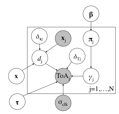
Figure 1: Graphical Model for ToA geo-localization.

In real cellular networks and unlike in typical 3GPP simulation models [6], the NLOS biases are not Gaussian distributed, the distribution is not identical for all APs and in repeated trials the bias does not significantly change. Also, the cellular network are a far departure from the hexagonal idealization, especially in metropolitan areas. This combination in real cellular networks severely biases the localization accuracy, therefore necessitating that we model each source of error–the errors are larger than simulation predictions and not reducible by repeated trials.

III Probabilistic ToA model

In Fig. 1, we depict the graphical model for ToA localization. In this model, we have combined the quantization error, the thermal noise and the clock error in a single unbiased variable with known variance, $\sigma_{clk}^{2}$. Specifically, the model is described as follows:

$$\text{ToA}_{j}|d_{j},\tau,\delta_{T_{j}},\gamma_{j},\sigma^{2}_{clk} \sim\mathcal{N}(\tau+d_{j}+\gamma_{j}+\delta_{T_{j}},\sigma^{2}_{clk})$$ (3)

$$\gamma_{j}|\bm{\pi}_{j}\sim\text{Cat}(\bm{\pi}_{j})\qquad \qquad\bm{\pi}_{j}|\bm{\beta}\sim\text{Dir}(\bm{\beta})$$ (4)

$$\delta_{T_{j}}\sim\mathcal{N}(0,\sigma_{\delta_{T}}^{2})\qquad \qquad\delta_{\bar{{\mathbf{x}}}_{j}}\sim\mathcal{N}(0,\sigma_{\delta_{\mathbf{x}}}^{2})$$ (5)

where $d_{j}=||{\mathbf{x}}-(\bar{{\mathbf{x}}}_{j}+\delta_{\bar{{\mathbf{x}}}_{j}})||$ and the prior over ${\mathbf{x}}$ and $\tau$ is defined in Subsection III-B. The prior over the NLOS bias is discussed in the following subsection.

III-A Prior over the non-line-of-sight bias

The NLOS bias is due to the multiple paths the signal can take to travel from the transmitter to the receiver. If the paths are sufficiently apart in time, we refer to them as resolvable mulipath. If the paths are not separable, then they are considered unresolvable multipath and we can only estimate a ToA for all the paths clustered together in time. The estimated ToA is a weighted sum of all the individual ToAs for all the unresolvable paths. The paths are resolvable if the time difference between them is larger than the inverse of the bandwidth of the signal. In cellular LTE, the bandwidth of positioning signals is typically 10MHz and the unresolvable multipath can add tens of meters to the estimate of the ToA, even when the LOS path is present in the detected signal.

To model the NLOS bias distribution, we use a discrete random variable. We assume that $\gamma_{j}$ can take the values $\ell\sigma_{clk}/10$ for $\ell=0,1,\ldots$ with probability $\pi_{j\ell}$. The spacing of $\sigma_{clk}/10$ is chosen to be somewhat arbitrary. It just needs to be small enough with respect to the clock standard deviation so the discreteness of the distribution is not a limiting factor. In our experiments, we have placed a fixed distribution over $\bm{\pi}_{j}$, which is based on the standard behavior of NLOS biases [18], that allows us to provide accurate localization directly. We have set:

$$\bm{\pi}_{j\ell}=\begin{cases}\frac{1}{2K},&0\leq\ell<K\\ \frac{L-\ell+K-1}{L(L-1)},&K\leq\ell<L+K\\ 0,&\ell\geq L+K\end{cases}$$ (6)

This model assumes that 50% of NLOS biases are between 0 and $K$, which models the effect of the unresolvable NLOS bias over the LOS component. In the other 50% of the other cases, the LOS path is not present and the NLOS bias can be as large as $L$. In LTE, if we set $\sigma_{clk}$ to 10 meters, then $K=30$ assumes that the unresolvable NLOS bias can be as large as 30 meters, and setting $L=2000$ assumes the NLOS bias can be as large as 2 km, because the spacing in $\bm{\pi}_{j}$ is measured in intervals of $\sigma_{clk}/10$.

III-B Prior over the position of the object

We need an effective prior distribution over $\mathbf{x}$ and $\tau$, because the NLOS bias can be as large as hundreds of meters. If the distribution over the NLOS bias allows for hundreds of meters and we are using TDoA localization in which $\tau$ is unknown, an unrestricted prior over $\mathbf{x}$ and $\tau$ would assign high probability to solutions far from where the APs are situated and, in many cases, outside the convex hull of the APs.

Any prior directly over $\mathbf{x}$ and $\tau$ may end up being too restrictive or too wide if it also depends on the APs that have already been heard. This restricts the universal applicability of this procedure. Our adopted solution is simple and quite effective. Instead of putting a prior over $\mathbf{x}$ and $\tau$, we place a prior over $d_{j}$. We assume, a priori, that $d_{j}$ is uniformly distributed over the positive real numbers though other priors could be placed on this quantity as well [20].

As $d_{j}$ measures the range (in polar coordinates) from the object to the APs, we penalize positions that are further away from the APs that have been heard by the object when we translate this distance into Cartesian coordinates. This means that the localization is typically within the convex hull of the APs, but it can also be outside of it if needed. With this prior, the posterior over $\mathbf{x}$ and $\tau$ becomes:

$$p(\mathbf{x},\tau|-)\propto\prod_{j=1}^{N}\sum_{\ell=0}^{L}\pi_{j,\ell}\frac{\exp\left(-\frac{(\text{ToA}_{j}-\tau-d_{j}-\delta_{T_{j}}-\ell\sigma_{clk}/10)^{2}}{2\sigma_{clk}^{2}}\right)}{\sqrt{2\pi\sigma_{clk}^{2}}(d_{j}+\sigma_{clk})}.$$ (7)

$d_{j}$ appears in the denominator when we transform the uniform prior for $d_{j}$ into the Cartesian coordinate system over $\mathbf{x}$. We add $\sigma_{clk}$ to avoid the singularity at the AP locations. In most cases, $d_{j}\gg\sigma_{clk}$ and this value is only to avoid numerical instabilities. To perform posterior inference in this model, we rely on an expectation propagation procedure detailed in the following section.

IV Inference

Expectation propagation (EP) [8, 21, 22, 23] is a technique in Bayesian machine learning for approximating posterior beliefs with a simpler set of exponential family distributions. Consider a family of Gaussian distributions which factorizes as follows:

$$q({\mathbf{x}}) =\frac{1}{{Z_{\text{EP}}}}\prod_{j=1}^{{N}}\exp({\bm{\alpha}}_{j}^{T}{\mathbf{x}}-\frac{1}{2}{\mathbf{x}}^{T}{\bm{\Lambda}}_{j}{\mathbf{x}}),$$ (8)

where ${\bm{\alpha}}_{j}\in\mathbb{R}^{{N}}$ and ${\bm{\Lambda}}_{j}$ is a $3\times 3$ symmetric positive semi-definite matrix. Note that given $({\bm{\alpha}}_{j},{\bm{\Lambda}}_{j})$, $j=1,\ldots,N$, $q({\mathbf{x}})$ is a Gaussian distribution with covariance matrix and mean given by

$$\bm{\Sigma}_{\text{EP}}=\left(\sum_{j=1}^{{N}}{\bm{\Lambda}}_{j}\right)^{-1},~{}\bm{\mu}_{\text{EP}}=\bm{\Sigma}_{\text{EP}}\left(\sum_{j=1}^{{N}}{\bm{\alpha}}_{j}\right).$$ (9)

Our aim is to find $\underline{\bm{{\bm{\Lambda}}}}^{*}=[{\bm{\Lambda}}^{*}_{j}]_{j=1}^{N}$ and $\underline{\bm{\gamma}}=[{\bm{\alpha}}^{*}_{j}]_{j=1}^{N}$ such that $\left(\bm{\mu}_{\text{EP}},\bm{\Sigma}_{\text{EP}}\right)$ in (9) are an accurate estimate to the mean and covariance matrix of ${\mathbf{x}}$ w.r.t. the distribution in (7). In the supplementary material, we describe an algorithm that iteratively refines the parameters vectors ${\bm{\alpha}}_{j}$, ${\bm{\Lambda}}_{j}$ independently, so the update can be parallelized over $j=1,\ldots,N$. Our experiments have shown that the resulting algorithm typically converges to a stationary point in a few iterations, where the complexity is $\mathcal{O}(N)$ per iteration. Also, convergence is independent of the EP initialization, so we simply initialize ${\bm{\alpha}}_{j}$ and ${\bm{\Lambda}}_{j}$, $j=1,\ldots,{N}$ so that $\bm{\mu}_{\text{EP}}$ is at the center of the scenario and $\bm{\Sigma}_{\text{EP}}$ is a diagonal matrix with individual variance equal to a few meters.

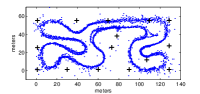
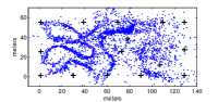
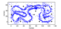
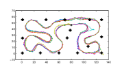
Figure 2: Raw localization for the 4650 transmissions for the second cart in (a) the performance of the proposed probabilistic algorithm. In (b) we show the least squares solution [10] and in (c) the nonlinear solution [9]. In (d) estimated position of the second cart using our probabilistic algorithm with a Kalman filter.

V Experiments

We have tested our algorithms using over-the-air ToA measurements for two different scenarios. The first scenario is a proprietary wireless network installed in an indoor go-cart track. The second scenario is a live LTE cellular network. We compare our proposed algorithm to the linear solution from [10] and the nonlinear solution from [9].

V-A Indoor Go-Cart Track

The first scenario consists of ToA measurements taken in an indoor go-cart race track approximately of area 120m $\times$ 80m. The location-awareness startup company Nanotron, in cooperation with go-cart system specialist SMS-Timing, installed Nanotron’s proprietary ToA localization system consisting of 15 APs. Two RF tags are attached to separate go-carts, and the two go-carts were driven simultaneously multiple times around the track. The system is an uplink system, where each go-cart tag transmits a known signal pulse of duration 4 $\mu$seconds and bandwidth 80MHz in the 2.4GHz unlicensed band, once every 100ms. The ToA is estimated at the APs. However, due to the limited range of the radios and interference, not all pulses are detected by all access points. The APs are synchronized through a proprietary Nanotron algorithm to achieve a standard deviation error below 1 meter. We have set $\sigma_{clk}=1$ meter, $K=40$ and $L=1500$.

The measurements from one go-cart are used to estimate the NLOS bias distributions, and the measurements from the second are used to measure the performance of the localization algorithms, as shown in Fig. 2(a). We note that we do not have the ground truth nor do we know the track layout, but we still are able to make a compelling case about the position on the karts based on the qualitative results of our model. We show the results for the linear algorithm [10] in (b), for the nonlinear algorithm [9] in (c), and for our probabilistic ToA algorithm in (a). For the linear algorithm, the circuit is not visible in the right hand side of the plot and the nonlinear algorithms looks like a nosier version of the solution proposed by our algorithm, in which the circuit is outlined accurately. For our algorithm only the top left straight path looks a bit noisier. The larger errors occur when the device has only been heard by fewer than 6 access points out of the 15 that are available.

We show the result for our probabilistic algorithm with a Kalman filter in Fig. 2. In this plot, we have joined the dots with lines of different colors for each loop around the circuit. In this plot, we can see that our algorithm clearly traces the cart going around the track. It also reveals detailed information about the driver performance. The driver’s lap time improves for the first three laps, but on the fourth lap (cyan) the cart veers off the track momentarily.

V-B Live LTE Networks

We present performance results based on ToA measurements taken from live LTE networks. Two sets of data are studied, each corresponding to a different metropolitan area in the United States. The first set shows how the performance of the probabilistic algorithm improves when more APs are heard (i.e., as $N$ increases), and the second set shows how estimating the biases of the APs can further improve the accuracy of the algorithm. In both cases, we set $\sigma_{clk}=20$ meters, $K=10$ and $L=1000$. The results for the second LTE network are reported in the Supplementary Material. In this second example we show how $\delta_{T_{j}}$ can be learnt in order to significantly reduced the localization biases.

V-B1 LTE Network A

For the first set of data, measurements are taken at 14 indoor locations within buildings around the downtown area of a large city. Two network configurations were employed: a standard configuration, and an enhanced configuration where the transmissions of the PRSs are coordinated to reduce interference and increase the number of APs heard. In the standard configuration, the average number of APs heard for a given transmission opportunity was $N=5$, and that value increases to 12 for the enhanced configuration.

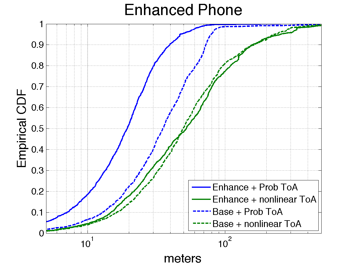
Figure 3: Empirical CDF localization error for an LTE cellular network over 14 indoor locations using 2 different networks configurations (solid versus dashed), and two localization algorithms (blue and green).

The ground truth is known precisely, so it is possible to measure the error of the localization algorithms. In Fig. 3, we show the empirical cumulative density function (CDF) for the localization error, in which the errors are sorted in the x-axis and the y-axis shows the proportion of transmissions that are below that error. For a given network configuration, 100 measurements are taken for each of the 14 locations, so each CDF curve consists of about 1400 points. For each network configuration, we consider the performance of the nonlinear algorithm and the proposed probabilistic algorithm.

We observe that the enhanced network does not change the performance of the nonlinear algorithm significantly. At the 90th percentile, the baseline algorithm performance is about 150m. The performance of the proposed probabilistic algorithm under the standard network configuration is uniformly better than that of the nonlinear algorithm. The 90th percentile error is reduced by about a factor of 2 to 72 meters. Increasing AP hearability with the enhanced network further reduces the error to 40 meters. Hence the probabilistic algorithm with the enhanced network operation improves the performance by a factor of 4 compared to the current baseline. The probabilistic algorithm achieves these gains because its NLOS model is able to detect the APs suffering from a strong NLOS bias and to reduce their effect in the location estimate.

VI Conclusions

We have proposed a probabilistic algorithm that can learn the biases corresponding to the two most significant sources of error in time-of-arrival localization using cellular networks. We then develop a novel multilateration algorithm by casting the localization problem as a probabilistic machine-learning problem in which all sources of error are accounted for. Using measurements from a live LTE network, we have shown that the proposed algorithm reduces the error by an order of magnitude–to less than 10 meters.

Supplementary Material

VI-A EP Iterative refinement

We first describe the update of the pair $({\bm{\alpha}}_{m},{\bm{\Lambda}}_{m})$ assuming that ${\bm{\alpha}}_{j}$, ${\bm{\Lambda}}_{j}$, for $j\neq m$ are fixed. The main idea is to remove the $m$-th factor, $\exp({\bm{\alpha}}_{m}^{T}{\mathbf{x}}-\frac{1}{2}{\mathbf{x}}^{T}{\bm{\Lambda}}_{m}{\mathbf{x}})$, from $q({\mathbf{x}})$ in (8) and include the associated “true” factor. The pair $({\bm{\alpha}}_{m},{\bm{\Lambda}}_{m})$ is updated according to the moments computed in this modified distribution. We define the cavity distribution as

$$q^{\backslash m}({\mathbf{x}})=\frac{1}{\hat{Z}^{\backslash m}}\prod_{\begin{subarray}{c}j=1\\ j\neq m\end{subarray}}^{{N}}\exp({\bm{\alpha}}_{j}^{T}{\mathbf{x}}-\frac{1}{2}{\mathbf{x}}^{T}{\bm{\Lambda}}_{j}{\mathbf{x}}),$$ (10)

and the tilted distribution as

$$p^{\backslash m}({\mathbf{x}}) \propto\sum_{\ell=0}^{L}\frac{\pi_{m,\ell}}{(d_{m}+\sigma_{clk})}p^{\backslash m,\ell}({\mathbf{x}})$$ (11)

where

$$\begin{split}p^{\backslash m,\ell}({\mathbf{x}})&\propto q^{\backslash m}({\mathbf{x}})\exp\left(\frac{-(\text{ToA}_{j}-\tau-d_{j}-\delta_{T}-\ell\sigma_{clk}/10)^{2}}{2\sigma_{clk}^{2}}\right)\end{split}$$

To update the pair $({\bm{\alpha}}_{m},{\bm{\Lambda}}_{m})$, we approximate the mean tilted distribution as follows:

$$\mathbb{E}_{p^{\backslash m}({\mathbf{x}})}\left[{\mathbf{x}}\right] \approx\frac{\displaystyle\sum_{\ell=0}^{L}\frac{\pi_{\ell}}{(d^{\ell}_{m}+\sigma_{clk})}~{}\mathbb{E}_{p^{\backslash m,\ell}({\mathbf{x}})}\left[{\mathbf{x}}\right]}{\displaystyle\sum_{q=0}^{L}\pi_{q}/(d^{q}_{m}+\sigma_{clk})},$$ (12)

$d^{\ell}_{m}$ is the Euclidean distance between the $m$-th AP and $\mathbb{E}_{p^{\backslash m,\ell}({\mathbf{x}})}\left[{\mathbf{x}}\right]$ is the mean of $p^{\backslash m,\ell}({\mathbf{x}})$. Note that we are replacing the $1/(d_{m}({\mathbf{x}})+\sigma_{clk})$ penalty term in (11) by its value at the mean of the inner distribution $p^{\backslash m,\ell}({\mathbf{x}})$. We can proceed similarly to estimate the correlation of the tilted distribution $\mathbb{E}_{p^{\backslash m}({\mathbf{x}})}\left[{\mathbf{x}}{\mathbf{x}}^{T}\right]$. Finally, the first two moments of $p^{\backslash m,\ell}({\mathbf{x}})$ are estimated by a Gaussian-quadrature approximation, in which we use a first order Taylor expansion of the term $d_{m}=\sqrt{||\mathbf{x}-\bar{\mathbf{x}}_{m}||^{2}}$ around the mean of the cavity distribution $q^{\backslash m}({\mathbf{x}})$, obtaining a Gaussian approximation to $p^{\backslash m,\ell}({\mathbf{x}})$. The updated pair $({\bm{\alpha}}^{*}_{m},{\bm{\Lambda}}^{*}_{m})$ is updated as follows:

$${\bm{\Lambda}}_{m}^{*} =\left(\text{CoVar}_{p^{\backslash m}({\mathbf{x}})}[{\mathbf{x}}]\right)^{-1}-\sum_{\begin{subarray}{c}j=1\\ j\neq m\end{subarray}}^{{N}}{\bm{\Lambda}}_{j}\qquad$$ (13)

$${\bm{\alpha}}_{m}^{*} :=\left(\text{CoVar}_{p^{\backslash m}({\mathbf{x}})}[{\mathbf{x}}]\right)^{-1}\mathbb{E}_{p^{\backslash m}({\mathbf{x}})}\left[{\mathbf{x}}\right]-\sum_{\begin{subarray}{c}j=1\\ j\neq m\end{subarray}}^{{N}}{\bm{\alpha}}_{j}.$$ (14)

VI-B LTE Network B

The experiment consists of two phases: a training phase where the calibration errors for the APs are estimated, and a testing phase where the probabilistic algorithm is run on the corrected ToAs. The network operated with the standard hearability. In the training phase, we took 100 measurements in a parking lot in order to estimate the calibration bias of nearby APs. We made the following three assumptions: all the ToA measurements were LOS; the reference AP did not have a bias; and all the calibration bias was due to cable length (i.e. $\delta_{{\mathbf{x}}_{j}}=0$). In this training location, we got a clear GPS reading and its location as the ground truth to estimate $\delta_{T_{j}}$ for each of the visible APs. We found that most APs had an error between 0 and 50 meters. In Fig. 5, we show the location of the APs. The ones in red numbered (1, 3, 5, 6, 7, 10 and 13) are the one that we see all the time in the training point. The other we see them infrequently and we cannot compensate their biases.

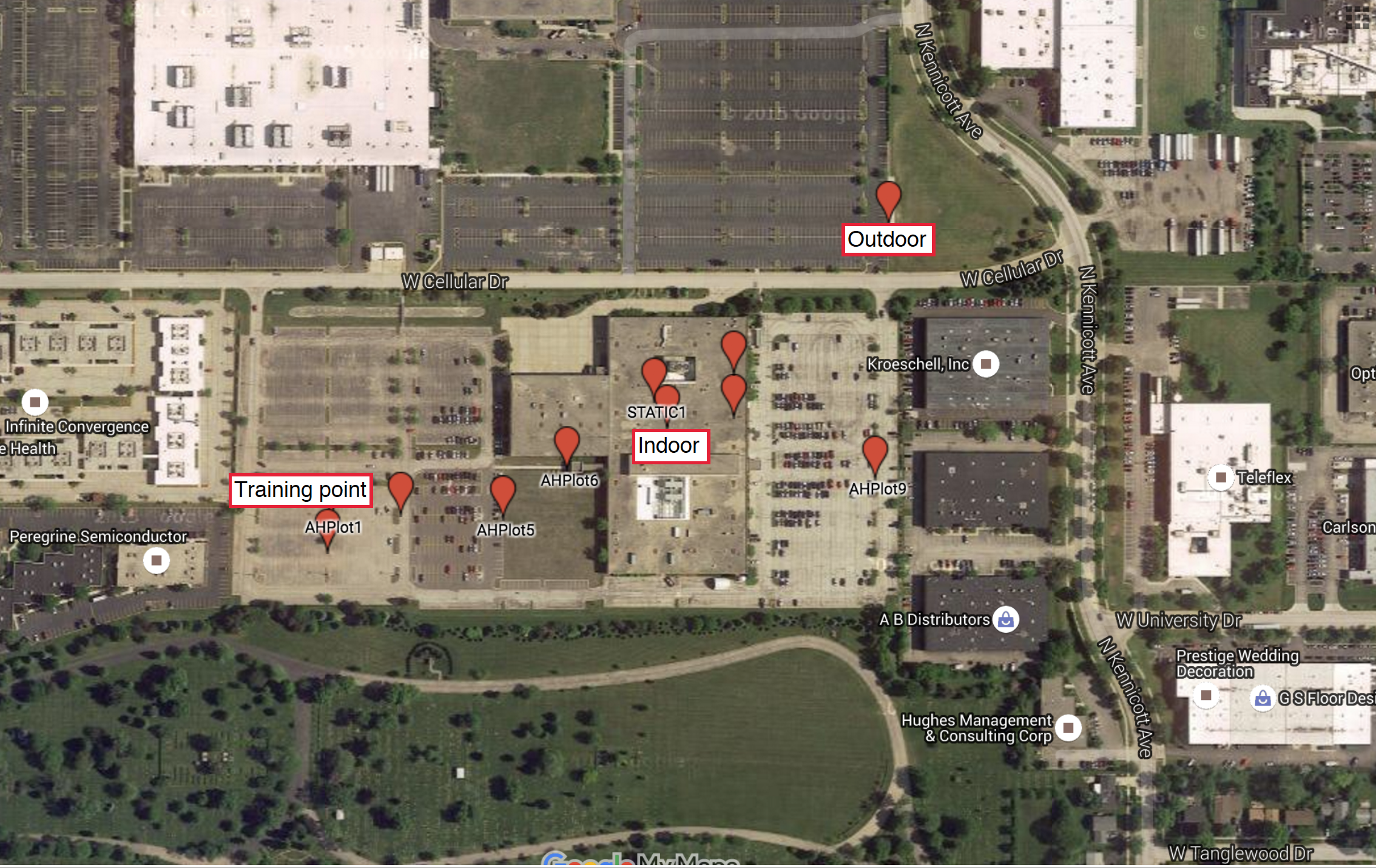
Figure 4: Satellite map for the position of the training and test point for LTE Network B.

Figure 5: Map for the position of the APs for LTE Network B. The green dots are the positions of the device from Fig. 4.

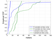
(a) Outdoor

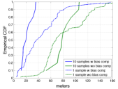
(b) Indoor

Figure 6: Empirical CDF localization error for a 100 measurements outdoor (a) and indoor (b).

In the testing phase, we took additional measurements at two nearby locations. One was in another parking lot (Fig. 4 labeled as Outdoor), and the second one was inside a building (Fig. 4 labeled as Indoor). The ToAs for AP $j$ was corrected using the estimated calibration error $\delta_{T_{j}}$. The empirical CDF localization error for both locations is shown in Fig. 6. It can be seen that once we compensate for the biases, the localization errors reduce considerably.

References

- [1] E. Günes and G. Ibarra, “IntraNav – low-cost indoor localization system & IoT platform,” in Microsoft Indoor Competition 2016, 2016.
- [2] W. Su, J. You, L. E, and R. Wang, “Precise indoor localization platform based on WiFiGeoMagnetic,” in Microsoft Indoor Competition 2016, 2016.
- [3] G. Lui, T. Gallagher, L. B. A. G. Dempster, and C. Rizos, “Differences in RSSI readings made by different WiFi chipsets: A limitation of WLAN localization,” in IEEE Int. Conf. Localization and GNSS (ICL-GNSS), 2011, pp. 53–57.
- [4] S. M. George, W. Zhou, H. Chenji, M. Won, Y. O. Lee, A. Pazarloglou, R. Stoleru, and P. Barooah, “DistressNet: a wireless ad hoc and sensor network architecture for situation management in disaster response,” IEEE Communications Magazine, vol. 48, no. 3, pp. 128–136, 2010.
- [5] T. S. Rappaport, J. H. Reed, and D. Woerner, “Position location using wireless communications on highways of the future,” IEEE Communication Maganize, vol. 34, no. 10, pp. 33–41, 1996.
- [6] Unknown, “Study on indoor positioning enhancements for UTRA and LTE,” 3rd Generation Partnership Project (TR 37.857) http://www.tech-invite.com/3m37/tinv-3gpp-37-857.html, Tech. Rep., 2015.
- [7] F. Perez-Cruz, C.-K. Lin, and H. Huang, “BLADE: A universal, blind learning algorithm for ToA localization in NLOS channels,” in IEEE 2016 Globecom Workshop, 2016.
- [8] T. Minka, “Expectation propagation for approximate Bayesian inference,” in Proceedings of the Seventeenth Conference on Uncertainty in Artificial Intelligence. Morgan Kaufmann Publishers Inc., 2001, pp. 362–369.
- [9] S. Fischer, “Observed time difference of arrival (OTDOA) positioning in 3GPP LTE,” Qualcomm Technologies, Tech. Rep., 2014.
- [10] I. Guvenc and C. C. Chong, “A survey on ToA based wireless localization and NLOS mitigation techniques,” IEEE Communications Survey & Tutorials, vol. 11, no. 3, pp. 107–124, 2009.
- [11] T. Sathyan, M. Hedley, and M. Mallick, “An analysis of the error characteristics of two time of arrival localization techniques,” in Proceedings of the 13th International Conference on Information Fusion, 2010.
- [12] R. M. Vaghefi and R. M. Buehrer, “Cooperative joint synchronization and localization in wireless sensor networks,” IEEE Transactions on Signal Processing, vol. 63, no. 14, pp. 3615–3627, 2015.
- [13] F. Ricciato, S. Sciancalepore, F. Gringoli, N. Facchi, and G. Boggia, “Position and velocity estimation of a non-cooperative source from asynchronous packet arrival time measurements,” IEEE Transactions on Mobile Computing, vol. 17, no. 9, pp. 2166–2179, 2018.
- [14] A. Coluccia and A. Fascista, “On the hybrid TOA/RSS range estimation in wireless sensor networks,” IEEE Transactions on Wireless Communications, vol. 17, no. 1, pp. 361–371, 2017.
- [15] S. Tomic and M. Beko, “A robust NLOS bias mitigation technique for RSS-TOA-based target localization,” IEEE Signal Processing Letters, vol. 26, no. 1, pp. 64–68, 2018.
- [16] S. Tomic, M. Beko, M. Tuba, and V. M. F. Correia, “Target localization in NLOS environments using RSS and TOA measurements,” IEEE Wireless Communications Letters, vol. 7, no. 6, pp. 1062–1065, 2018.
- [17] M. A. Lombardi, “Fundamentals of time and frequency,” in The Mechatronics Handbook, R. H. Bishop, Ed. CRC PRESS, 2002, ch. 17.
- [18] J. Medbo, I. Siomina, A. Kangas, and J. Furuskog, “Propagation channel impact on LTE positioning accuracy: A study based on real measurements of observed time difference of arrival,” in IEEE Int. Symp. Personal, Indoor and Mobile Radio Communications (PIMRC), 2009, pp. 2213 – 2217.
- [19] Y. W. Teh, M. I. Jordan, M. J. Beal, and D. M. Blei., “Hierarchical dirichlet processes,” Journal of the American Statistical Association, vol. 101, pp. 1566–1581, 2006.
- [20] A. Coluccia and F. Ricciato, “RSS-based localization via bayesian ranging and iterative least squares positioning,” IEEE Communications letters, vol. 18, no. 5, pp. 873–876, 2014.
- [21] M. W. Seeger, “Expectation propagation for exponential families,” Tech. Rep., 2005.
- [22] ——, “Bayesian inference and optimal design for the sparse linear model,” J. Mach. Learn. Res., vol. 9, pp. 759–813, Jun. 2008.
- [23] M. Opper and O. Winther, “Expectation consistent approximate inference,” J. Mach. Learn. Res., vol. 6, pp. 2177–2204, Dec. 2005.