Energy-Efficient Job-Assignment Policy with Asymptotically Guaranteed Performance Deviation

Abstract

We study a job-assignment problem in a large-scale server farm system with geographically deployed servers as abstracted computer components (e.g., storage, network links, and processors) that are potentially diverse. We aim to maximize the energy efficiency of the entire system by effectively controlling carried load on networked servers. A scalable, near-optimal job-assignment policy is proposed. The optimality is gauged as, roughly speaking, energy cost per job. Our key result is an upper bound on the deviation between the proposed policy and the asymptotically optimal energy efficiency, when job sizes are exponentially distributed and blocking probabilities are positive. Relying on Whittle relaxation and the asymptotic optimality theorem of Weber and Weiss, this bound is shown to decrease exponentially as the number of servers and the arrival rates of jobs increase arbitrarily and in proportion. In consequence, the proposed policy is asymptotically optimal and, more importantly, approaches asymptotic optimality quickly (exponentially). This suggests that the proposed policy is close to optimal even for relatively small systems (and indeed any larger systems), and this is consistent with the results of our simulations. Simulations indicate that the policy is effective, and robust to variations in job-size distributions.

I Introduction

Global Internet traffic is rapidly increasing, driving a parallel growth in the data-center industry; over 500 thousand data centers have been launched worldwide [1]. According to an estimate in 2013, about 91 billion kWh of electricity were consumed by U.S. data centers during that year, and the annual consumption has been predicted to reach $13 billion with nearly 100 million metric tons of carbon pollution, potentially, by 2020 [2]. Servers are considered to be the major contributor to the electrical consumption of data centers [3]. We study the dispatching policies for incoming jobs in a server farm consisting of deployed servers/computer components, aiming to maximize energy efficiency.

Energy-efficient scheduling policies for local server farms are well-studied. For instance, speed scaling technique can reduce energy consumption by decreasing server speed(s) [4, 5]; energy-efficient servers enable dynamic right-sizing of server farms by powering servers on/off/into power-conservative modes according to offered traffic load [6, 7]; and decision making policies according to queue sizes of servers have been considered by changing server working modes [8, 9]. The development of distributed cloud computing platforms has stimulated research on geographically deployed energy-efficient server farms [10, 11].

Server farm vendors deploy a variety of computer components, such as CPUs and disks, to meet various types of inquiries from Internet users, and different generations of these components are present simultaneously because of partial upgrading of old components and purchasing new ones over time [12]. A diversity of physical computing/storage components are available for use in cloud computing platforms, and are abstracted (virtualized) as resources with varying attributes [13]. All of these have resulted in heterogeneity as an important feature in attempting to undertake research on server farms, whereas [14, 15] studied only identical servers.

Regardless of the complexity caused by heterogeneity of server farms, large modern server farms with hundreds of thousands of computer components (abstracted servers) require all scheduling policies to be scalable.

Existing job-assignment policies have been discussed in server farms that have negligible energy consumption on idle servers [4, 16, 8, 17]. Power consumption on idle servers is normally significant in real situations [18], and we so regard it in this paper.

On the other hand, job-assignment policies for network resource allocation problems, such as [19, 20], applicable for practical scenarios with heterogeneous servers and jobs, were studied as static optimizations. Profits to be gained through dynamic release and reuse of resources were ignored. Here we use methods of stochastic optimization that capture dynamic properties of a system.

To maximize the energy efficiency, defined as the ratio of the long-run average throughput to the long-run average power consumption, in a stochastic system with heterogeneous servers, an asymptotically optimal job-assignment policy was proposed in [21]. This optimal policy approaches the optimal solution as the numbers of servers in different server groups tend to infinity proportionately. Nonetheless, the asymptotic optimality is restricted in two aspects: a) although modern server farms are normally large enough to be close to the asymptotic regime, the critical value, above which the numbers of servers are “sufficiently large”, remains unclear, and b) it was assumed that any server in the server farm can serve any arriving job if it has a vacant slot in its buffer. This constraint is not appropriate for geographically separated or functionally varied computer components (abstracted servers). A detailed survey of other published work is provided in Section II.

We aim to maximize the energy efficiency and study the deviation between a newly proposed, scalable policy and the true optimal solution; particularly studying the relationship between this deviation and the number of servers in the system. Also, we extend the idea of [21] to a more general, realistic system in which the available servers for a given job are, to some extent, job-dependent. This extension significantly complicates the entire system and enables consideration of the effects on the problem of the geographical locations and service features (e.g., CPU or memory) of computer components. This was not captured in [21]. We refer to the abstracted servers that are potentially able to serve a job as the available servers of this job.

The primary contribution of this paper is a sharpening of the asymptotic optimality results in a heterogeneous server farm, discussed in a special case in [21]. Specifically, we prove that, when the job sizes are exponentially distributed and the blocking probabilities of jobs are always positive, there is a hard upper bound on the deviation between a simple, scalable policy and the optimized energy efficiency in the asymptotic regime; this upper bound diminishes exponentially as the number of servers in server groups and the arrival rates of jobs tend to infinity proportionately. In other words, the scalable policy approaches asymptotic optimality quickly (exponentially) as the size of the optimization problem increases. We refer to this upper bound as the deviation bound, and the policy as Priorities accounting for Available Servers (PAS), as it is a priority-style policy and applicable for a system with different sets of available servers.

Our secondary contributions are twofold:

• We consider a large-scale system, potentially containing several geographically distributed server farms, and regard this hybrid system as an abstracted server farm model. We propose a scalable PAS policy in this server farm with heterogeneous servers and jobs, where energy consumption and service rates of servers can be arbitrarily related. As mentioned in our primary contribution, the PAS policy is proved to rapidly (exponentially) approach asymptotic optimality as the scale of the server farm increases. To the best of our knowledge, no existing work has studied the energy efficiency of such a realistically scaled heterogeneous server farm, nor does any existing work propose a scalable scheduling policy with proven guaranteed performance.

• By numerical simulations, we demonstrate that PAS is nearly optimal even for relatively small server farms. Together with the rapidly decreasing deviation bound, when job sizes are exponentially distributed and the blocking probabilities of jobs are always positive, it is likely to be near-optimal in all larger server farms and proved to approach optimality as the server farm sizes tend to infinity. In particular, the deviation bound of PAS is demonstrated to decrease with increasing server farm size, consistent with our theoretical results, and to be less than $3\%$ in all our experiments involving only 100 servers (computer components). Also, we numerically demonstrate that the PAS policy is relatively insensitive to the specific job-size distribution by comparing its energy efficiency with different job-size distributions.

The paper is organized as follows: Section II: discussion of related work on job assignment policies; Section III: description of the server farm model; Section IV: definition of the stochastic optimization problem; Section V: description of the PAS policy; Section VI: proof of the deviation bound; Section VII: numerical results; Section VIII: conclusions.

II Other Related Work

Asymptotically optimal job-assignment policies applicable to a parallel queueing model with infinite buffer size on each server were studied in [22, 23]. In [24, 25], policies were proposed for server farms without capacity constraints (with infinite buffer size), aimed at minimization of average delay. A detailed survey of asymptotically optimal job-assignment policies was given in [21].

In particular, the asymptotic results presented in this paper are obtained by implementing the Whittle relaxation technique, which was originally designated for the restless multi-armed bandit problem (RMABP) [26]. The optimization of a general RMABP was proved to be PSPACE-hard [27]; nonetheless, in [28], a scalable policy, proposed through the Whittle relaxation technique and referred to as the (Whittle) index policy in [26], was proved to be asymptotically optimal under conditions that require a global attractor of a stochastic process associated with the RMABP, and Whittle indexability [26]. There is not a necessary implication between one of these conditions and asymptotic optimality. In [29, 30], Niño-Mora proposed and analyzed the Partial Conservation Law (PCL) indexability for the performance of scheduling problems, such as the (restless) multi-armed bandit problem. This implies (and is stronger than) the Whittle indexability. A More detailed survey about indexability can be found in [31].

Other publications that discuss management of jobs in server farms by distributing offered traffic were published recently [5, 10]. Lenhart et al. [5] provided an experimental analysis on energy-efficient web servers with an assumption of a cubic relationionship between server power consumption and traffic load. The number of servers (nodes) tested in [5] is very small compared to a real system in modern data centers. Lin et al. [10] analyzed energy efficiency performance in communication networks in a server farm model. They assumed power consumption is negligible on idle servers (multiplexing/aggregating nodes in network). Recall that, here, we allow the possibility of positive power consumption on idle.

An auction based mechanism was studied in a server farm model with heterogeneous servers (resources) and job types (users) in [11]. The authors provided a worst-case ratio (competitive ratio) of the revenue (social welfare) under their proposed policies relative to the optimal solution, and showed it to be linearly increasing in the time horizon. Also, in [11], the length of each job is assumed known before assigning it. Here, we consider the more realistic situation that the job length remains unknown until it is completed.

Stochastic job-assignment techniques were studied in [32], where a linearly increasing relationship of reward/cost rates to traffic loads of servers is assumed. They proposed a reasonable and scalable policy with a given parameter $V$ and proved the deviation between this policy and the optimal solution to be $O(1/V)$, where $V$ is a parameter related to the Lyapunov optimization technique. For the version of energy-efficient server farms considered here, the energy consumption rate of computer components is generally non-linear in its traffic load, so the linearity is not appropriate for modeling energy consumption rates of computer components in Cloud environments. In consequence, the results in [32] are not directly applicable to the energy-efficient server farm.

In [32], the blocking of jobs was allowed when not all servers are fully occupied. Also, a deterministic job lifespan model was assumed and all server were assumed to be able to handle all jobs. We strictly prohibit blocking of jobs when available servers are not fully occupied, to ensure the fairness for all customers. We also consider a diversity of jobs with randomly generated job sizes (remaining unknown until completed) and with job-dependent sets of available servers.

In summary, the non-linearity of power functions and the complexity of our server farm model prevent applicability of existing methods from being direct. Also, there is no published work that provided theoretical bounds that are quickly (exponentially) decreasing in the number of servers between proposed policy and the optimal solution.

Moreover, as mentioned in Section I, powering servers on/off [14, 6, 15] or switching into power conservative modes with additional suspending time [7, 8, 32, 10] enables dynamic variation of the size/number of working of working servers in a server farm. In [6, 15], such server farms are called dynamic right-sizing server farms. In similar vein to [16, 17, 21], for the purposes of this paper, a fixed number of working servers is postulated in a server farm with no possibility of powering off or state switching, with substantial delay, during the time period under consideration. In practice, this corresponds to periods during which no powering off or state switching, with concomitant substantial delays, takes place. In this context, the job assignment policies discussed here can be combined with the right-sizing techniques, as appropriate. Note that frequent powering off/on or state switches increases wear and tear of hardware and ensuing requirements for costly replacement and maintenance [33].

III Model

We classify incoming jobs into $J$ job types labeled by an integer $j$ ($j=1,\ldots,J$), each of which has an arrival rate $\lambda_{j}>0$ indicating the average number of arrivals per unit time, following a Poisson process as previous studies in Cloud environments [34, 35]. If groups/type of Internet/network customers decide to send requests independently and identically during a given time period and the number of such customers is sufficiently large for the corresponding dynamic process to become stationary, then it is reasonable to model the arrival process of customer requests for this type as a Poisson process, although the arrival rates may vary from one time period to another, which is consistent with observations of real-world tracelogs [36, 37].

These jobs will be undertaken by servers or blocked. We classify the servers into different server groups according to their functional features and profiles. Define the set of server groups as $\mathcal{K}\coloneqq\{1,2,\ldots,K\}$. We assume that there are in total $K\geq 2$ server groups and $R_{k}\geq 1$ servers in group $k$. Each job type $j$ is only able to be served by a server from a subset $\emptyset\neq\mathcal{K}_{j}\subset\mathcal{K}$ of server groups. We say that $k\in\mathcal{K}_{j}$ is an available server group for job type $j$ and a server of group $k$ is an available server for a job of type $j$. A server’s availability of serving different jobs can be affected by its functional features, jobs’ preferences, and geographical distances from the jobs.

The sizes of jobs of the same type are independent identically distributed (i.i.d.) with average job size normalized to be one (bit). We assume, for convenience, i.i.d. job sizes across all job types for the theoretical development, but we provide numerical results in Section VII to indicate the robustness of our results when when job-size distributions vary across job types.

A server of group $k$ serves its jobs at a total and peak rate of $\mu_{k}$ using the processor sharing (PS) service discipline. When the server is not idle, the service rate received by each job is then $\mu_{k}$ divided by the number of jobs in the server buffer. The service rate of each server in group $k$ is supported by consuming non-negligible amount of energy, even in its idle mode. Similarly, we assume that each server operates in a power-consuming mode with its peak energy consumption rate when there are jobs accommodated. We refer to this peak energy consumption rate as the energy consumption rate of a busy server, denoted by $\varepsilon_{k}$ for group $k=1,2,\ldots,K$. When the server is idle, it automatically changes to a power-conservative mode and consumes $\varepsilon_{k}^{0}$ energy per unit time. Evidently, $\varepsilon_{k}>\varepsilon_{k}^{0}\geq 0$. The service rates and energy consumption rates of busy/idle servers are intrinsic parameters determined by the server hardware features and profiles, and the relationship between them can be arbitrary in this paper.

As in [6, 8, 16, 17, 21], the busy/idle operating rule is more appropriate to machines working in two-power modes, such as Oracle Sun Fire X2270 M2, Cisco UCS C210, Cisco MXE 3500 and Cisco UCS 5108. Also, the IEEE 802.11 standards define exactly two power saving modes for network components in energy-conservative communications.

Moreover, we study a system with finite service capacity on each server, referred to as its buffer size. It provides a finite bound on the number of jobs being simultaneously served by this server. Let $B_{k}\geq 1$ represent the buffer size of a server in group $k$.

A policy $\phi$ is a mechanism to assign an arriving job of type $j$ to a server of group $k\in\mathcal{K}_{j}$ with at least one vacant slot in its buffer. A fairness criterion requires equal treatment of the different job types. In particular, rejection of jobs sent by different users is not permitted if there are vacant slots on available servers. If there is no such server (all available buffers are fully occupied), the arriving job is lost.

Consider a ratio of total arrival rate to the total service rate, i.e., $\rho\coloneqq\sum_{j\in\mathcal{J}}\lambda_{j}/\sum_{k\in\mathcal{K}}\mu_{k}$, the normalized offered traffic (see [21]). For a specific job type $j$, the normalized offered traffic of type $j$, $\rho_{j}\coloneqq\lambda_{j}/\sum_{k\in\mathcal{K}_{j}}\mu_{k}$.

We assume the existence of long-run averages of throughput and power consumption, and refer to them as the job throughput and the power consumption of the system, respectively. Precise definitions are given in Section IV. We define $\mathcal{L}^{\phi}$ and $\mathcal{E}^{\phi}$ to be the job throughput and power consumption of the system under policy $\phi$, respectively. The energy efficiency of policy $\phi$, $\mathcal{L}^{\phi}/\mathcal{E}^{\phi}$, is the objective of our problem for energy-efficient server farms. The value of the energy efficiency indicates the average job throughput achieved by consuming one unit energy. Since we do not permit rejection of jobs when there are vacancies on available servers, the objective encapsulates a trade-off between performance and energy consumption.

IV Stochastic Optimization Problem

We study a stochastic system, where the dynamically released service capacities of physical components can be reused. To capture the stochastic features, we start by introducing the stochastic state of the entire system: a server farm with tens of thousands of heterogeneous servers.

Define the state of an individual server as the number of jobs currently on the server. The set of all possible states of a server of group $k\in\mathcal{K}$, is denoted by $\mathcal{B}_{k}=\{0,1,\ldots,B_{k}\}$, where $B_{k}\geq 1$. As in [21], states $0,1,\ldots,B_{k}-1$ are called controllable, and the state $B_{k}$ is uncontrollable, since all new jobs will be rejected by a server in state $B_{k}$. Denote the set of all controllable states of server group $k$ by $\mathcal{C}_{k}=\{0,1,\ldots,B_{k}-1\}$ and that of the uncontrollable states by $\mathcal{U}_{k}=\{B_{k}\}$.

Servers of the same group have potentially different states in the stochastic process. Define the set of servers in group $k$ as $\mathcal{R}_{k}$. The set of all servers is $\mathcal{S}\coloneqq\bigcup_{k\in\mathcal{K}}\mathcal{R}_{k}$, the set of servers available for jobs of type $j\in\mathcal{J}$ is $\mathcal{S}_{j}\coloneqq\bigcup_{k\in\mathcal{K}_{j}}\mathcal{R}_{k}$, and the state space of the entire system is $\mathcal{B}\coloneqq\prod_{k\in\mathcal{K}}(\mathcal{B}_{k})^{R_{k}}$. The size of the state space thus increases exponentially in the number of servers in the server farm, i.e., $|\mathcal{S}|$, which, in itself, is normally very large in modern real server farms.

Decisions driven by a stationary policy $\phi$ applied to job arrivals rely on the state of the system just before an arrival occurs and the information known in this state, such as average rates of transitioning to other states. For a policy $\phi$, $s\in\mathcal{S}$, $j\in\mathcal{J}$, we define the action variable $a^{\phi}_{j,s}(\bm{n})\in\{0,1\}$, $\bm{n}\in\mathcal{B}$, to indicate the decision under policy $\phi$ for an arriving job of type $j$ on server $s$ in state $\bm{n}$: server $s$ accepts an arriving job of type $j$ if $a^{\phi}_{j,s}(\bm{n})=1$; and does not accept any job otherwise. In this context, for each job of type $j$, there is at most one server $s$ with $a^{\phi}_{j,s}(\bm{n})=1$ among all available servers.

In addition, we define, for $\bm{n}\in\mathcal{B}$, $j\in\mathcal{J}$, $s\in\mathcal{S}$,

• $a^{\phi}_{j,s}(\bm{n})\equiv 0$ if $s\notin\mathcal{S}_{j}$ to prevent a server that is unavailable for job type $j$;

• $a^{\phi}_{j,s}(\bm{n})\equiv 0$ if $n_{s}=B_{k}$, $s\in\mathcal{R}_{k}$, $k\in\mathcal{K}_{j}$, to prevent a server from accepting a new job when it is fully occupied.

Then, the action space, as the discrete set of possible values of the action variables, is

$$\mathcal{A}\coloneqq\prod_{j\in\mathcal{J}}\{0,1\}^{\sum_{k\in\mathcal{K}_{j}}R_{k}},\vspace{-0.2cm}$$ (1)

where we recall that $\mathcal{K}_{j}$ is the set of available server groups for job type $j$ and $R_{k}$ is the number of servers in group $k$. With large number of servers $R_{k}$, multiple job types (i.e., $J>1$) significantly enlarge the number of action variables in parallel with the size of the action space.

Let $N_{s}^{\phi}(t)\in\mathcal{B}_{k}$, $s\in\mathcal{R}_{k}$, $k\in\mathcal{K}$, represent the state of server $s$ at time $t$ under policy $\phi$, and $\bm{N}^{\phi}(t)=(N^{\phi}_{s}(t):s\in\mathcal{S})\in\mathcal{B}$. For simplicity, we always consider an empty system at time $0$, $\bm{N}^{\phi}(0)=\bm{0}$.

It will be convenient to consider mappings $\bm{f}=(f_{1},f_{2},\ldots,f_{K})$, where $f_{k}:\mathcal{B}_{k}\rightarrow\mathbb{R}$, We refer to such a vector of mappings $\bm{f}\in\prod_{k\in\mathcal{K}}\mathbb{R}^{\mathcal{B}_{k}}$ as the vector of reward rate functions. Then, for a given $\bm{f}\in\prod_{k\in\mathcal{K}}\mathbb{R}^{\mathcal{B}_{k}}$, for some $k$, we define the long-run average performance of the system under policy $\phi$ to be

$$\Gamma^{\phi}(\bm{f})=\lim\limits_{t\rightarrow+\infty}\frac{1}{t}\mathbb{E}\left[\int_{0}^{t}\sum\limits_{k\in\mathcal{K}}\sum\limits_{s\in\mathcal{R}_{k}}f_{k}(N^{\phi}_{s}(u))du\right],$$ (2)

where we assume the existence of such limit.

Specifically, we define $f^{\mu}_{k}(n_{k})$ and $f^{\varepsilon}_{k}(n_{k})$, $n_{k}\in\mathcal{B}_{k}$, $k\in\mathcal{K}$, as the service rate and energy consumption rate of a server in group $k$ in state $n_{k}$, respectively, and consider them as the reward rate functions; that is, for $k\in\mathcal{K}$, $f^{\mu}_{k}$ and $f^{\varepsilon}_{k}$ are mappings: $\mathcal{B}_{k}\rightarrow\mathbb{R}$. As defined in Section III, $f^{\mu}_{k}(n_{k})=\mu_{k}$, $f^{\varepsilon}_{k}(n_{k})=\varepsilon_{k}$ for $n_{k}>0$, $f^{\mu}_{k}(0)=0$ and $f^{\varepsilon}_{k}(0)=\varepsilon_{k}^{0}$, where $\mu_{k}>0$, $\varepsilon_{k}>\varepsilon_{k}^{0}\geq 0$, $k\in\mathcal{K}$. For the vectors $\bm{f}^{\mu}=(f^{\mu}_{1},f^{\mu}_{2},\ldots,f^{\mu}_{K})$ and $\bm{f}^{\varepsilon}=(f^{\varepsilon}_{1},f^{\varepsilon}_{2},\ldots,f^{\varepsilon}_{K})$, the job throughput of the entire system is, then, $\Gamma^{\phi}(\bm{f}^{\mu})$, and the power consumption of the system is $\Gamma^{\phi}(\bm{f}^{\varepsilon})$. Recall that our objective is to maximize the energy efficiency of the entire system; that is, $\mathcal{L}^{\phi}/\mathcal{E}^{\phi}=\Gamma^{\phi}(\bm{f}^{\mu})/\Gamma^{\phi}(\bm{f}^{\varepsilon})$.

To complete necessary constraints on the action variables of our optimization problem, there remain definitions to accommodate behavior that blocks an arriving job. We define a virtual server group $0$ with server number $R_{0}=1$ and server set $\mathcal{R}_{0}=\{1\}$, which receives blocked jobs. Any server of group $0$ has only one state with zero transition rate all the time: that is, it does not generate any reward or cost to the entire system. We define $\mathcal{B}_{0}$ as the state space of a server of group $0$ where $|\mathcal{B}_{0}|=1$. Also, the set of controllable states for $0$ is set to be $\mathcal{C}_{0}=\mathcal{B}_{0}$ and the one for uncontrollable states is $\mathcal{U}_{0}=\emptyset$.

We extend the original definition of a policy $\phi$ determined by actions $a^{\phi}_{j,s}(\bm{n})$ ($\bm{n}\in\mathcal{B},\ s\in\mathcal{S},\ j\in\mathcal{J}$), to that determined by actions $(a^{\phi}_{j,s}(\bm{n})$: $\bm{n}\in\mathcal{B},\ s\in\mathcal{S},\ j\in\mathcal{J};\ a^{\phi}_{j}(\bm{n}))$, where $a^{\phi}_{j}(\bm{n})\in\{0,1\}$ represents the action variable for the only server of virtual group $0$ for job type $j$. We slightly abuse the notation and still use $\phi$ to denote such a policy.

Let $k(s)$ be the label of the server group satisfying $s\in\mathcal{R}_{k(s)}$, and $I(x)$ be the Heaviside function: for $x\in\mathbb{R}$, $I(x)=1$ if $x>0$; and $0$ otherwise. Define $\Theta(x)=xI(x)$, $x\in\mathbb{R}$. Our problem is then encapsulated by

$$\max_{\phi}\Gamma^{\phi}(\bm{f}^{\mu})/\Gamma^{\phi}(\bm{f}^{\varepsilon})\vspace{-0.2cm}$$ (3)

with policy $\phi$ subject to

$$\sum\limits_{s\in\mathcal{S}_{j}}a^{\phi}_{j,s}\bigl{(}\bm{N}^{\phi}(t)\bigr{)}+\Theta\Bigl{(}\overline{a}^{\phi}_{j}\bigl{(}\bm{N}^{\phi}(t)\bigr{)}\Bigr{)}=1,\forall j\in\mathcal{J},t\geq 0,$$ (4)

$$\overline{a}^{\phi}_{j}(\bm{N}^{\phi}(t))+\sum\limits_{s\in\mathcal{S}_{j}}I\left(B_{k(s)}-N^{\phi}_{s}(t)\right)\leq 1,\forall j\in\mathcal{J},t\geq 0,\vspace{-0.3cm}$$ (5)

by introducing variables $\overline{a}^{\phi}_{j}(\bm{n})\in\mathbb{R}$ and setting $a^{\phi}_{j}(\bm{n})=\Theta(\overline{a}^{\phi}_{j}(\bm{n}))$, $\bm{n}\in\mathcal{B}$. Define $\Phi$ to be the set of all the policies $\phi$ satisfying (4) and (5). Constraints in (5) and variables $\overline{a}^{\phi}_{j}(\bm{n})$ are introduced to guarantee that jobs of type $j$ are blocked if and only if all the available servers are fully occupied:

• if all available servers for job type $j$ are fully occupied at time $t$, then, because all available servers are in uncontrollable states, $a^{\phi}_{j,s}(\bm{N}^{\phi}(t))=0$ for all $s\in\mathcal{S}_{j}$ and the constraint in (4) forces $a^{\phi}_{j}(\bm{N}^{\phi}(t))=\Theta(\overline{a}^{\phi}_{j}(\bm{N}^{\phi}(t)))=1$, which does not violate the constraint in (5);

• otherwise, the constraint in (5) forces $\overline{a}^{\phi}_{j}(\bm{N}^{\phi}(t))\leq 0$, which leads to $a^{\phi}_{j}(\bm{N}^{\phi}(t))=\Theta(\overline{a}^{\phi}_{j}(\bm{N}^{\phi}(t)))=0$ and so a newly-arrived job of type $j$ cannot be blocked.

We aim at a largely scaled problem that exhibits inevitably high computational complexity. A special case of our problem is in fact an instance of the Restless Multi-Armed Bandit Problem (RMABP) [26]. The RMABP has been proved to be PSPACE-hard [27] in the general case, so that near-optimal, scalable approximations are the impetus to this paper. Here, we consider a general case involving not only heterogeneous servers, but also heterogeneous jobs, which is much more practical and significantly increases the size of the action space, as described in (1). In particular, different sets of available servers for different jobs enable consideration of geographically distributed servers, jobs’ preferences and functional differences among servers.

V Priority-Style Policy

As mentioned in Section I, in [21], a policy that always prioritizes the most efficient servers was proposed and proved to approach the optimality when the problem size (number of servers) becomes arbitrarily large; in other words, it is asymptotically optimal. However, this policy requires that the set of available servers for each job always include all servers in the server farm, and the asymptotic optimality is not applicable in a realistic system with a large but finite number of servers. It is important to know the detailed relationship between the performance degradation and the problem size.

Recall our objective of maximizing the energy efficiency of the entire server farm, defined as the ratio of the job throughput to the power consumption. The power consumption can be interpreted as the cost used to support corresponding job throughput. In this context, for an idle server in group $k\in\mathcal{K}$, $\varepsilon_{k}^{0}$ units of power are consumed in support of a zero service rate; if the server becomes busy, $\varepsilon_{k}-\varepsilon_{k}^{0}$ power is added to produce a service rate $\mu_{k}$ .

In other words, the idle power $\varepsilon_{k}^{0}$ is a persistent and uncontrollable cost producing no service rate; while, $\varepsilon_{k}-\varepsilon_{k}^{0}$ is the productive and controllable part of the power that serves jobs at service rate $\mu_{k}$. We propose a policy that always prioritizes servers producing higher service rates per unit controllable power; namely, the ratio of its service rate to the productive part of its power consumption, $\mu_{k}/(\varepsilon_{k}-\varepsilon_{k}^{0})$. The ratio was referred to as the effective energy efficiency in [21].

In particular, for an incoming job of type $j\in\mathcal{J}$ with a set of available servers $\mathcal{S}_{j}$, the job will be assigned to a server in $\mathcal{S}_{j}$ with highest effective energy efficiency and with at least one vacancy in its buffer. As indicated earlier, we refer to such a policy as the Priorities accounting for Available Servers (PAS). Note that PAS uses a similar idea to that proposed in [21], but is applicable for our problem with different sets of available servers.

Input : The server $s\in\mathcal{S}$ where an arrival occurs at time $t$.

Function UpdatingUponArrival($s$):

       for $j\in\mathcal{J}$ with $s\in\mathcal{S}_{j}$ do

             Remove $s$ from the max heap $\mathcal{H}_{j}(t)$

             $\upsilon_{j}(t)\leftarrow$ the root node of the updated $\mathcal{H}_{j}(t)$

            

       end for

      

return

Algorithm 1 Updating the indication vector upon an arrival.

For $j\in\mathcal{J}$, let $\mathcal{N}^{\{0\}}_{j}=\left\{\bm{n}\in\mathcal{B}\left|\forall s\in\mathcal{S}_{j},n_{s}\in\mathcal{U}_{k(s)}\right.\right\}$ and $\mathcal{N}^{\{0,1\}}_{j}=\left\{\bm{n}\in\mathcal{B}\left|\exists s\in\mathcal{S}_{j},n_{s}\in\mathcal{C}_{k(s)}\right.\right\}$. Rigorously, the action variables for PAS are given by

$$a_{j,s}^{\text{PAS}}(\bm{n})=\left\{\begin{cases}1,&\text{ if $\bm{n}\in\mathcal{N}_{j}^{\{0,1\}}$ and }\\ &\text{$s\in\arg\max_{s\in\mathcal{S}_{j}:n_{s}\in\mathcal{C}_{k(s)}}\Bigl{[}\frac{\mu_{k(s)}}{\varepsilon_{k(s)}-\varepsilon_{k(s)}^{0}}\Bigr{]}$},\\ 0,&\text{ otherwise}.\vspace{-0.2cm}\end{cases}\right.$$ (6)

If $\arg\max[\cdot]$ returns a set with more than one element, ties can be broken arbitrarily. We set, without loss of generality, policy PAS to always select the smallest $s$ among the set of value(s) returned by this $\arg\max[\cdot]$.

For clarity, we provide an example of implementing PAS. Maintain a indication vector $\bm{\upsilon}(t)\in\mathcal{S}^{|\mathcal{J}|}$ at time $t$, where the $j$th element $\upsilon_{j}(t)$ represents the server used to accommodate a newly-arrive job of type $j$ if it arrives at time $t$. Note that, $a^{\text{PAS}}_{j,s}(\cdot)$ can be determined by $\bm{\upsilon}(t)$ by setting $a^{\text{PAS}}_{j,s}(\cdot)=1$ for $s=\upsilon_{j}(t)$ and $0$ for others. For each job type $j\in\mathcal{J}$, maintain a max heap $\mathcal{H}_{j}(t)$ of servers $s\in\mathcal{S}_{j}$ with respect to the effective energy efficiency $\mu_{k(s)}/(\varepsilon_{k(s)}-\varepsilon_{k(s)}^{0})$. If a server $s$ transitions from $B_{k(s)}-1$ to $B_{k(s)}$ or from $B_{k(s)}$ to $B_{k(s)}-1$, we trigger a potential update of the indication vector and the max heaps for all types, as described in Algorithms 1 and 2, respectively. For both algorithms, the worst-case computational complexity is $O(\sum_{j\in\mathcal{J}}\log|\mathcal{S}_{j}|)$ and the space complexity is $O(\sum_{j\in\mathcal{J}}|\mathcal{S}_{j}|)$, representing the storage space for the vector $\bm{\upsilon}(t)$ and heaps $\mathcal{H}_{j}(t)$ ($j\in\mathcal{J}$).

Note that the PAS policy does not require $\lambda_{j}$ to be known nor, indeed, do we assume specific distributions for the inter-arrival/inter-departure times. In other words, PAS is widely applicable and scalable to a server farm with heterogeneous servers and jobs.

Input : The server $s\in\mathcal{S}$ where a departure occurs at time $t$.

Function UpdatingUponDeparture($s$):

       for $j\in\mathcal{J}$ with $s\in\mathcal{S}_{j}$ do

             Add $s$ in the max heap $\mathcal{H}_{j}(t)$

             $\upsilon_{j}(t)\leftarrow$ the root node of the updated $\mathcal{H}_{j}(t)$

            

       end for

      

return

Algorithm 2 Updating the indication vector upon a departure.

VI Deviation Analysis

Following similar ideas in [28, 21], in this section, we obtain an upper bound for the performance deviation between PAS and the optimal solution in asymptotic regime, under certain condition. We refer to this upper bound as the deviation bound. The deviation bound diminishes exponentially in the size of the system leading, in particular, to asymptotic optimality of PAS.

Following the idea in [26], servers should be prioritized according to their potential profits, quantized and obtained by relaxing the constraint of the optimization problem. This is referred to as the Whittle relaxation technique. Our problem, (3)-(5), is treated similarly.

This technique produces a highly intuitive heuristic scheduling policy, which coincides with PAS under certain conditions. We prove this equivalence in Section VI-A. Based on this equivalence, in Section VI-B, we prove that the deviation bound of PAS’s performance is diminishing rapidly (in fact, exponentially) as the problem size increases.

VI-A Whittle Relaxation

From [16, Theorem 1], if $\Gamma^{\phi}(\bm{f}^{\mu})<+\infty$ and $\Gamma^{\phi}(\bm{f}^{\varepsilon})<+\infty$ for all $\phi\in\Phi$, and we define,

$$e^{*}=\max\limits_{\phi\in\Phi}\left\{\Gamma^{\phi}(\bm{f}^{\mu})/\Gamma^{\phi}(\bm{f}^{\varepsilon})\right\},\vspace{-0.1cm}$$ (7)

then a policy optimizes the problem described by equations (3)-(5) if and only if it optimizes

$$\max\limits_{\phi}\left\{\Gamma^{\phi}(\bm{f}^{r})\right\},\ \text{s. t. \eqref{eqn:org:constraint_1} and \eqref{eqn:org:constraint_2},}\vspace{-0.3cm}$$ (8)

where the vector of reward rate functions $\bm{f}^{r}\in\prod_{k\in\mathcal{K}}\mathbb{R}^{\mathcal{B}_{k}}$ is defined by

$$f^{r}_{k}(n_{k})=f^{\mu}_{k}(n_{k})-e^{*}f^{\varepsilon}_{k}(n_{k}),$$ (9)

for $n_{k}\in\mathcal{B}_{k}$, $k\in\mathcal{K}$. Let

$$\alpha^{\phi}_{j}=\lim\limits_{t\rightarrow+\infty}\mathbb{E}[a^{\phi}_{j}(\bm{N}^{\phi}(t))]=\lim\limits_{t\rightarrow+\infty}\mathbb{E}\left[\Theta\left(\overline{a}^{\phi}_{j}(\bm{N}^{\phi}(t))\right)\right]$$

and

$$\overline{\alpha}^{\phi}_{j}=\lim\limits_{t\rightarrow+\infty}\mathbb{E}\left[\overline{a}^{\phi}_{j}(\bm{N}^{\phi}(t))\right].$$

The Whittle relaxation technique involves randomization of the action variables $a^{\phi}_{j,s}(\cdot)$ and $\overline{a}^{\phi}_{j}(\cdot)$. This relaxation of (3)-(5) produces the following problem:

$$\max\limits_{\phi}\Gamma^{\phi}(\bm{f}^{r})\vspace{-0.3cm}$$ (10)

subject to

$$\sum\limits_{s\in\mathcal{S}_{j}}\lim\limits_{t\rightarrow+\infty}\mathbb{E}\left[a^{\phi}_{j,s}\left(\bm{N}^{\phi}(t)\right)\right]+\alpha^{\phi}_{j}=1,~{}\forall j\in\mathcal{J},$$ (11)

$$\overline{\alpha}^{\phi}_{j}+\sum\limits_{s\in\mathcal{S}_{j}}\lim\limits_{t\rightarrow+\infty}\mathbb{E}\left[I\left(B_{k(s)}-N^{\phi}_{s}(t)\right)\right]\leq 1,~{}\forall j\in\mathcal{J}.$$ (12)

The relaxed problem no longer captures the server farm problem realistically, but is useful for theoretical analysis. Define

$$A_{j}=\sum_{s\in\mathcal{S}_{j}}\sum_{n\in\mathcal{C}_{k(s)}}\pi_{s}^{*}(n),~{}j\in\mathcal{J},$$

where $\pi^{*}_{s}(n)$ is the steady-state probability of state $n$ for server $s$ under policy $\phi$ satisfying $a^{\phi}_{j^{\prime},s^{\prime}}(\bm{n}^{\prime})=1$ for all $\bm{n}^{\prime}\in\mathcal{B}$, $n^{\prime}_{s^{\prime}}\in\mathcal{C}_{k(s^{\prime})}$, $j^{\prime}\in\mathcal{J}$ and $s^{\prime}\in\mathcal{S}_{j^{\prime}}$. It is clear that, for $j\in\mathcal{J}$,

$$A_{j}\leq\sum\limits_{s\in\mathcal{S}_{j}}\lim\limits_{t\rightarrow+\infty}\mathbb{E}\left[I\left(B_{k(s)}-N^{\phi}_{s}(t)\right)\right].$$

In this context, Equation (12) can be relaxed further to

$$\Theta(\overline{\alpha}_{j}^{\phi})\leq\Theta(1-A_{j}),\ \forall j\in\mathcal{J}.$$ (13)

To complete the analysis, we introduce, for the relaxed problem defined by (10),(11) and (13), a redundant constraint:

$$\lim\limits_{t\rightarrow\infty}\mathbb{E}\bigl{[}a^{\phi}_{j,s}(\bm{N}^{\phi}(t))|\ N^{\phi}_{s}=B_{k(s)}\bigr{]}=0,\left\{\begin{array}[]{l}\forall j\in\mathcal{J},\\ \forall s\in\mathcal{S}_{j},\end{array}\right.$$ (14)

which forces the action varibles for the uncontrollable states to be zero. Constraints (11), (13) and (14) can be combined with the objective function by introducing Lagrangian multipliers $\bm{\nu}$, $\bm{\gamma}$ and $\bm{\eta}$ corresponding to (11), (13) and (14), respectively. Let $\tilde{\Phi}$ represent the set of all stationary policies. Define

1. $\pi_{s}^{\phi}(n)$, $s\in\mathcal{S}$, $n\in\mathcal{B}_{k(s)}$, $\phi\in\tilde{\Phi}$, as the steady state probability of server $s$ in state $n$ under policy $\phi$;

2. row vector $\bm{\pi}^{\phi}_{s}=(\pi^{\phi}_{s}(n):\ n\in\mathcal{B}_{k(s)})$, $s\in\mathcal{S}$, $\phi\in\tilde{\Phi}$;

3. column vector $\bm{f}^{r}_{s}=(f^{r}_{s}(n):\ n\in\mathcal{B}_{k(s)})$, $s\in\mathcal{S}$;

4. column vector $\bm{\alpha}^{\phi}_{j,s}=(\alpha^{\phi}_{j,s}(n):\ n\in\mathcal{B}_{k(s)})$ where

   $$\alpha^{\phi}_{j,s}(n)=\lim\limits_{t\rightarrow+\infty}\mathbb{E}\left[a^{\phi}_{j,s}(\bm{N}^{\phi}(t))|\ N^{\phi}_{s}(t)=n\right],$$

   $j\in\mathcal{J}$, $s\in\mathcal{S}_{j}$, $\phi\in\tilde{\Phi}$;

5. column vector $\bm{e}^{n}$, $n\in\mathbb{N}^{+}$, of size $n$ with all zero elements except the $n$th element set to be one.

The Lagrange problem with respect to the primal problem defined by (10), (11), (13) and (14) is then

$$\Lambda(\bm{\nu},\bm{\gamma},\bm{\eta})=\\ \max\limits_{\phi}\sum\limits_{s\in\mathcal{S}}\bm{\pi}_{s}^{\phi}\Bigl{(}\bm{f}^{r}_{s}-\sum\limits_{j\in\mathcal{J}_{s}}\nu_{j}\bm{\alpha}^{\phi}_{j,s}-\sum\limits_{j\in\mathcal{J}_{s}}\eta_{j,s}\alpha^{\phi}_{j,s}(B_{k(s)})\bm{e}^{B_{k(s)}}\Bigr{)}\\ -\sum\limits_{j\in\mathcal{J}}(\nu_{j}\alpha^{\phi}_{j}+\gamma_{j}\Theta(\overline{\alpha}^{\phi}_{j}))+\sum\limits_{j\in\mathcal{J}}\left(\nu_{j}+\gamma_{j}\Theta(1-A_{j})\right)$$ (15)

where $\mathcal{J}_{s}=\{j\in\mathcal{J}|\ s\in\mathcal{S}_{j}\}$, $s\in\mathcal{S}$.

As in [26], given $\bm{\nu}$, $\bm{\gamma}$ and $\bm{\eta}$, the maximization problem at the right hand side of (15) achieves the same maximum as a sum of the maximum values of $|\mathcal{S}|+J$ independent sub-problems: for $s\in\mathcal{S}$,

$$\max\limits_{\phi\in\Phi_{s}}\bm{\pi}_{s}^{\phi}\bigl{(}\bm{f}^{r}_{s}-\sum\limits_{j\in\mathcal{J}_{s}}\nu_{j}\bm{\alpha}^{\phi}_{j,s}-\sum\limits_{j\in\mathcal{J}_{s}}\eta_{j,s}\alpha^{\phi}_{j,s}(B_{k(s)})\bm{e}^{B_{k(s)}}\bigr{)}\vspace{-0.2cm}$$ (16)

where $\Phi_{s}$ represents the set of stationary policies $\phi$ determined by action variables $\alpha^{\phi}_{j,s}(n)\in[0,1]$, $n\in\mathcal{B}_{k(s)}$, $j\in\mathcal{J}$; and for $j\in\mathcal{J}$,

$$\max\limits_{\phi\in\overline{\Phi}_{j}}-\nu_{j}\alpha^{\phi}_{j}-\gamma_{j}\Theta(\overline{\alpha}^{\phi}_{j}),\vspace{-0.2cm}$$ (17)

where $\overline{\Phi}_{j}$ is the set of stationary policies $\phi$ determined by action variables $\overline{\alpha}^{\phi}_{j}$ and $\alpha^{\phi}_{j}$. Remarkably, the dimension of the state space for each of these independent sub-problems is $1$.

Condition 1.

For all $j\in\mathcal{J}$, $A_{j}\leq 1$.

We refer to Condition 1 as the heavy traffic condition: the blocking probabilities for jobs are almost positive all the time.

Proposition 1.

When the job sizes are exponentially distributed, if either $J=1$ or Condition 1 holds true, then there exists a $\nu\in\mathbb{R}$ and a policy $\phi^{*}\in\Phi$ that maximizes the relaxed problem defined by (10), (11), (13) and (14), satisfying, for $j\in\mathcal{J}$,

1. if $s\in\mathcal{S}_{j}$, $n\in\mathcal{C}_{k(s)}$,

   $$\alpha^{\phi^{*}}_{j,s}(n)=\left\{\begin{cases}1,&\text{if }\nu<1-e^{*}\frac{\varepsilon_{k(s)}-\varepsilon_{k(s)}^{0}}{\mu_{k(s)}}\\ 1\text{ or }0,&\text{if }\nu=1-e^{*}\frac{\varepsilon_{k(s)}-\varepsilon_{k(s)}^{0}}{\mu_{k(s)}},\\ 0,&\text{if }\nu>1-e^{*}\frac{\varepsilon_{k(s)}-\varepsilon_{k(s)}^{0}}{\mu_{k(s)}};\end{cases}\right.$$ (18)

2. and

   $$\alpha^{\phi^{*}}_{j}=1-\sum\limits_{s\in\mathcal{S}_{j}}\sum\limits_{n\in\mathcal{C}_{k(s)}}\pi^{\phi^{*}}_{s}(n)\alpha^{\phi^{*}}_{j,s}(n).$$ (19)

The proof of Proposition 1 is given in Appendix A.

Note that although we can calculate the optimal solution of the relaxed problem, referred to as policy $\phi^{*}$ in Proposition 1, such $\phi^{*}$ is not applicable to the original problem that we are really interested in. Nevertheless, $\phi^{*}$ does offer interesting intuitions that help us construct a scalable, near-optimal heuristic policy applicable to the original problem. In the following, we explain and construct this heuristic policy and prove its equivalence to PAS.

For $j\in\mathcal{J}$, $s\in\mathcal{S}_{j}$, $n\in\mathcal{C}_{k(s)}$, let

$$\nu^{*}_{j,k(s)}(n)=1-e^{*}\frac{\varepsilon_{k(s)}-\varepsilon_{k(s)}^{0}}{\mu_{k(s)}}.$$ (20)

The optimal policy $\phi^{*}$ described in (18) implies the priorities of different servers: for a given $\nu$, if job-server pair $(j,s)$ has $\alpha^{\phi^{*}}_{j,s}(n)=1$, $n\in\mathcal{C}_{k(s)}$, then any other pairs $(j,s^{\prime})$ with $\nu^{*}_{j,k(s^{\prime})}(n^{\prime})>\nu^{*}_{j,k(s)}(n)$ must have $\alpha^{\phi^{*}}_{j,s^{\prime}}(n^{\prime})=1$, $n^{\prime}\in\mathcal{C}_{k(s^{\prime})}$. The value of $\nu^{*}_{j,k(s)}(\cdot)$ can be interpreted as the server’s potential profits (or subsidy following the idea in [26]) gained by choosing this server $s$ to serve a job of type $j$ if this server is not fully occupied.

A similar property was defined in [26] for a Restless Multi-Armed Bandit Problem (RMABP) and referred to as Whittle indexability. When job sizes are exponentially distributed, $J=1$ and neglecting (5), our problem reduces to a RMABP, and Whittle indices are given by $\nu^{*}_{j,k(s)}(\cdot)$. There may be no simple closed form for the Whittle indices in the general case with general job-size distributions. Relevant work about RMABP and Whittle indices have been mentioned in Section II.

In the general case, if we always assign incoming jobs of type $j$ to servers with the highest $\nu^{*}_{j,k(s)}(\cdot)$, for the highest potential profits, among those in the available set $\mathcal{S}_{j}$ and with vacancies in their buffers, then the resulting policy coincides with PAS described in Section V. PAS is applicable to the original problem, defined by (3)-(5). We discuss PAS in Section VI-B by comparing it to policy $\phi^{*}$ described in Proposition 1. If $\phi^{*}$ is optimal for the relaxed problem, then the performance of $\phi^{*}$ is an upper bound of that of the original problem. If PAS’s performance again coincides with $\phi^{*}$, then PAS is optimal for the original problem.

VI-B Convergence in Performance

VI-B1 Stochastic Processes with Smooth Trajectories

Let states $n\in\mathcal{C}_{k}$ for all $k\in\mathcal{K}$ be ordered according to descending values $\nu^{*}_{j,k}(n)$, where uncontrollable states $n\in\mathcal{U}_{k}$, for all $k\in\mathcal{K}$, follow the controllable states in the ordering, with $\alpha^{\phi}_{j,s}(n)=0$ for $n\in\mathcal{U}_{k}$, $s\in\mathcal{R}_{k}$, $k\in\mathcal{K}_{j}$, $j\in\mathcal{J}$. Then we place the state $n\in\mathcal{B}_{0}$ of zero-reward servers, also a controllable state, after all other controllable states but preceding the uncontrollable states. To indicate the order of states, the position of a state in the ordering $i=1,2,\ldots,I$, where $I=\sum_{k\in\mathcal{K}\cup\{0\}}|\mathcal{B}_{k}|$, is regarded as its label. Define $\tilde{\mathcal{B}}\coloneqq\{1,2,\ldots,I\}$. Let $n_{i}$ represent the server state labeled by $i$ (i.e., the $i$th state), and $k_{i}$ represent the only server group with $n_{i}\in\mathcal{B}_{k_{i}}$.

Since each $i\in\tilde{\mathcal{B}}$ is associated with a server group $k$ and a state in $\mathcal{B}_{k}$, servers are thus distinguishable only through their current state $i\in\tilde{\mathcal{B}}$.

Let $\bm{Z}^{\phi}(t)=(Z^{\phi}_{i}(t):\ i\in\tilde{\mathcal{B}})$, and $\mathcal{Z}$ represent the space of all probability vectors of length $I$. The random variable $Z_{i}^{\phi}(t)$ represents the proportion of servers in state $i\in\tilde{\mathcal{B}}$ at time $t$ under policy $\phi\in\Phi$, $t\geq 0$: that is,

$$Z_{i}^{\phi}(t)\coloneqq\frac{1}{|\mathcal{S}|+R_{0}}\left|\left\{s\in\mathcal{S}\ \right.\left|\ N_{s}^{\phi}(t)=i\right\}\right|.$$

Define a mapping $m$ by $m(\bm{N}^{\phi}(t))=\bm{Z}^{\phi}(t)$. Recall that our server farm is assumed to be empty at $t=0$, and, correspondingly, define $\bm{z}^{0}\coloneqq\bm{Z}^{\phi}(0)=m(\bm{0})$. On the arrival or departure of jobs at time $t$, $\bm{Z}^{\phi}(t)$ transitions to $\bm{Z}^{\phi}(t)+\bm{e}_{i,i^{\prime}}$, where $\bm{e}_{i,i^{\prime}}$ is a vector of which the $i$th element is $+1/(|\mathcal{S}|+R_{0})$, the $i^{\prime}$th element is $-1/(|\mathcal{S}|+R_{0})$ and otherwise is zero, $i,i^{\prime}\in\tilde{\mathcal{B}}$. Servers in server group $k$ only appear in state $n_{i}\in\mathcal{B}_{k}$; that is, the transition from $\bm{Z}^{\phi}(t)$ to $\bm{Z}^{\phi}(t)+\bm{e}_{i,i^{\prime}}$, $n_{i}\in\mathcal{B}_{k}$, $n_{i^{\prime}}\in\mathcal{B}_{k^{\prime}}$, $k,k^{\prime}\in\mathcal{K}\cup\{0\}$, $k\neq k^{\prime}$ never occurs.

Let $R_{k}=R_{k}^{0}h$ and $\lambda_{j}=\lambda_{j}^{0}h$, where $h=1,2,\ldots$ is called the scaling parameter. Correspondingly, let $S_{0}\coloneqq(|\mathcal{S}|+R_{0})/h$, then $S_{0}\in\mathbb{N}^{+}$. Since servers in the same state $i\in\tilde{\mathcal{B}}$ are indistinguishable, we define the probability of selecting/activating a server in state $i$ for an arriving job of type $j$, i.e., the probability of setting $\alpha^{\phi}_{j,s}(i)=1$, as $u^{\phi,h}_{j,i}(\bm{z})$, when policy $\phi$ is used, and $\bm{Z}^{\phi}(t)=\bm{z}$. Clearly, $u^{\phi,h}_{j,i}(\bm{z})=0$ and $\bm{z}\in\mathcal{Z}$, if $i$ represents an uncontrollable state.

We obtain, for $i\in\tilde{\mathcal{B}}$, $j\in\mathcal{J}$, $h\in\mathbb{N}^{+}$, $\bm{z}\in\mathcal{Z}$ with $z_{i}>0$,

$$u^{\text{PAS},h}_{j,i}(\bm{z})=\min\biggl{\{}1,\frac{1}{z_{i}}\max\Bigl{\{}0,\frac{1}{hS_{0}}-\sum\limits_{i^{\prime}<{i},k_{i^{\prime}}\in\mathcal{K}_{j}}z_{i^{\prime}}\Bigr{\}}\biggr{\}}.$$

We define without loss of generality the transition caused by an arrival event in state $i$ as the transition from state $i$ to state $i+1$, if $n_{i},n_{i+1}\in\mathcal{C}_{k}$, $k\in\mathcal{K}$. Such a transition from $i$ to $i+1$ is caused by an arrival of a job of a specified type.

Following the ideas of [28, 21, 38], we then obtain a corollary of [38, Proposition 5] as follows.

Corollary 1.

When the job sizes are exponentially distributed, for any $\delta>0$, there exists a $\bm{z}^{\text{PAS}}\in\mathcal{Z}$ such that

$$\lim\limits_{h\rightarrow+\infty}\lim\limits_{t\rightarrow+\infty}\frac{1}{t}\int_{0}^{t}\mathbb{P}\Bigl{\{}\bigl{\lVert}\bm{Z}^{\text{PAS},h}(u)-\bm{z}^{\text{PAS}}\bigr{\rVert}>\delta\Bigr{\}}du=0,$$ (21)

with given $\bm{Z}^{\text{PAS},h}(0)=\bm{z}^{0}$.

Equation (21) indicates that stochastic process $\bm{Z}^{\text{PAS},h}(t)$ will go into a close neighborhood of point $\bm{z}^{\text{PAS}}$ as the scaling parameter $h$ tends to infinity, where the process transition rates of leaving and entering each of its states must be equivalent. Also, since priorities of states are driven by $u^{\text{PAS},h}_{j,i}(\cdot)$, if we start from an empty server farm, the trajectory of $Z^{\text{PAS},h}_{i}(t)$, $t\geq 0$, is independent from the trajectories of $Z^{\text{PAS},h}_{i^{\prime}}(t)$, $t\geq 0$, for states $i^{\prime}>i$ (that is, states with lower priorities). We can then calculate the value of $\bm{z}^{\text{PAS}}$ from the first element to the last, which coincides with the calculating procedure of $\lim_{h\rightarrow+\infty}\lim_{t\rightarrow+\infty}\mathbb{E}[\bm{Z}^{\phi^{*},h}(t)]$ under $\phi^{*}$ with the state priorities driven by action variables described in (18) and (19).

Given the reward rate functions for all states $i\in\tilde{\mathcal{B}}$, the long-run average reward $\Gamma^{\phi}(\bm{f}^{r})$ (the objective function of our problem) of policy $\phi$ is linear in the expected value $\lim_{t\rightarrow+\infty}\mathbb{E}\bm{Z}^{\phi,h}(t)$. In other words, when $\bm{Z}^{\text{PAS},h}(t)$ approaches $\bm{z}^{\text{PAS}}$ in the asymptotic regime, $\Gamma^{\text{PAS}}(\bm{f}^{r})$ also approaches $\Gamma^{\phi^{*}}(\bm{f}^{r})$ for any given $e^{*}\in\mathbb{R}$. As mentioned at the end of Section VI-A, if $\phi^{*}$ is also optimal for the relaxed problem, then PAS is asymptotically optimal in the original problem, because the maximized energy efficiency of the relaxed problem is always an upper bound of that of the original one.

In consequence, if $J=1$ or Condition 1 is satisfied, Proposition 1 and Corollary 1 yield the asymptotic optimality of PAS as $h\rightarrow+\infty$ in terms of energy efficiency, when job sizes are exponentially distributed.

VI-B2 Bounded Performance Deviation

According to our result on asymptotic optimality stated in Section VI-B1, the performance deviation between PAS and the optimal solution in the asymptotic regime is directly related to the supremum of Euclidean distances between $\lim_{t\rightarrow+\infty}\mathbb{E}\bm{Z}^{\text{PAS},h}(t)$ and $\bm{z}^{\text{PAS}}$.

Proposition 2.

When the job sizes are exponentially distributed, for any $\delta>0$, there exist $\bm{z}^{\text{PAS}}\in\mathcal{Z}$, $s>0$ and $H>0$, such that, for any $h>H$,

$$\lim\limits_{t\rightarrow+\infty}\frac{1}{t}\int_{0}^{t}\mathbb{P}\Bigl{\{}\bigl{\lVert}\bm{Z}^{\text{PAS},h}(u)-\bm{z}^{\text{PAS}}\bigr{\rVert}>\delta\Bigr{\}}du\leq e^{-sh},\vspace{-0.2cm}$$ (22)

where $\bm{Z}^{\text{PAS},h}(0)=\bm{z}^{0}$.

The proof of Proposition 2 is given in Appendix B. That is, the deviation bound of PAS diminishes exponentially in the scaling parameter $h$.

As mentioned in Section I, since the asymptotic regime can never be achieved in the real world, Proposition 2 sharpens the asymptotic optimality result: PAS approaches asymptotic optimality very quickly (exponentially) as the problem size increases. Simulation results will be provided in Section VII.

Proposition 2 applies in systems with much more general power functions, extending asymptotic optimality of PAS to more general cases. For instance, by [38, Proposition 1] and Proposition 2, the PAS family is also asymptotically optimal when the service and energy consumption rates of each server is linearly increasing in the number of jobs there, although the linearity is not appropriate in modeling power consumption in Cloud environments. As mentioned in Section II, the problem studied here is already sufficiently complex to prevent existing methods from being applied directly. More general power functions will presumably and significantly complicate the system model and notational definitions and is outside the scope of this paper.

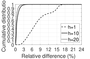
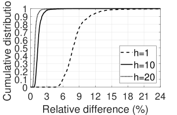
Figure 1: Cumulative distribution of the normalized performance deviation of the PAS policy: (a) single job type; (b) multiple job types.

VII Numerical Results

Here, we numerically demonstrate the effectiveness of PAS by comparing it with the optimal energy efficiency, as a benchmark, in different scenarios with randomly generated server farm systems. We recall that, as mentioned in Sections I and II, the complexity of the server farm model prevents applicability of existing scheduling policies from being direct.

In our simulation results, the $95\%$ confidence intervals based on the Student $t$-distribution are maintained within $\pm 3\%$ of the observed mean. In Sections VII-A and VII-B, we set job-sizes to be exponentially distributed, and in Section VII-C, more realistic job-size distributions are discussed.

VII-A Deviation Studies

We are interested in the performance deviation of the PAS policy; that is, how large the system should be to guarantee a performance deviation with reasonable bounds. For the sake of simplicity, let OPT represent an optimal solution for the relaxed problem defined by (10), (11), (13) and (14) in the asymptotic regime, we define the normalized performance deviation of a policy $\phi\in\Phi$, to be

$$\Bigl{(}\mathcal{L}^{\rm OPT}/\mathcal{E}^{\rm OPT}-\mathcal{L}^{\phi}/\mathcal{E}^{\phi}\Bigr{)}/\Bigl{(}\mathcal{L}^{\rm OPT}/\mathcal{E}^{\rm OPT}\Bigr{)}.$$

Note that energy efficiency under OPT is an upper bound for that under an optimal solution of the original problem defined by (3)–(5) in the asymptotic regime. Because of the extremely high computational complexity of the original problem, we use OPT as a benchmark in our numerical experiments.

VII-A1 Stochastically Identical Jobs

We start with the simple case of only one job type ($J=1$). Consider a server farm with five server groups ($K=5$), each of which has $R_{k}^{0}=1$, $k\in\mathcal{K}$, servers when the scaling parameter $h=1$. Let the buffer sizes $B_{k}$ of all servers equal 2, for all $k\in\mathcal{K}$. In Figure 1, we depict the cumulative distribution of the normalized performance deviation of PAS in terms of energy efficiency, with randomly generated service rates, energy consumption rates and sets of available servers as follows.

• Service rates $\mu_{k}$, $k\in\mathcal{K}$, are randomly uniformly generated in the range $[1,10]$;

• Energy efficiencies of servers in the first group are normalized to be 1, i.e., $\mu_{1}/\varepsilon_{1}=1$; those in successive groups are obtained by randomly uniformly generating the ratio of server energy efficiencies for successive groups, i.e., $(\mu_{k}/\varepsilon_{k})/(\mu_{k-1}/\varepsilon_{k-1})$, $k=2,3,\ldots,K$, from $[0.5,1]$ iteratively;

• According to the service rates and energy efficiencies of servers for different groups, we obtain the busy power consumption for all servers, and set the idle power of servers in group $k$, $k\in\mathcal{K}$, to be $\varepsilon_{k}\cdot(0.1+0.1\cdot k)$;

• All servers in the server farm are available for incoming jobs $\mathcal{K}_{1}=\mathcal{K}$; and

• The average arrival rate $\lambda_{1}$ is set to $\rho\cdot\sum_{k=1}^{K}\mu_{k}$ with a given normalized offered traffic $\rho$.

In Figure 1, the value of the normalized performance deviation of the PAS policy is decreasing in $h$, $h=1,10,20$, and, for all our simulations, is within $3\%$ (of the energy efficiency under OPT) when $h=20$; that is, twenty servers in each server group. In other words, in this experiment, the PAS policy is already close to OPT when the server farm is relatively small. These results are consistent with the deviation upper bound described by (22). That is, PAS is demonstrated to be near-optimal since the scaling parameter is relatively small, and, in line with our theoretical results (22), is likely to be near optimal for any larger $h$.

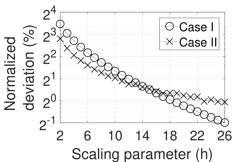
Figure 2: Performance of the PAS policy against the scaling parameter.

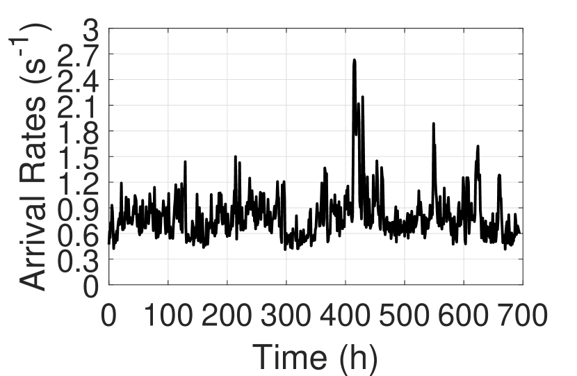
Figure 3: Arrival rates of Google trace-logs.

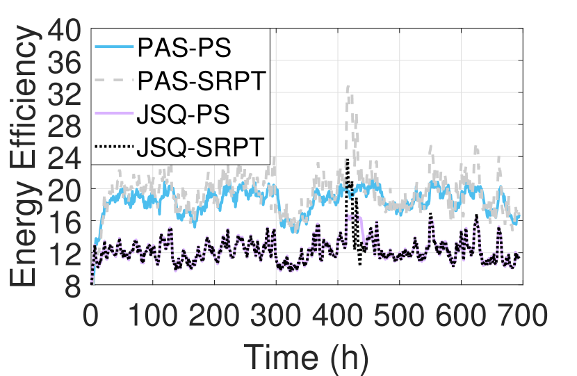
Figure 4: Energy efficiency of PAS and JSQ.

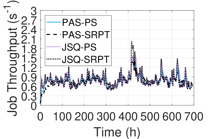
Figure 5: Job throughput of PAS and JSQ.

VII-A2 Multiple Job Types

For the general case of multiple job types, we define servers with the same settings as those for Figure 1 except here we set $B_{k}=1$ for $k\in\mathcal{K}$. We plot the cumulative distribution of normalized performance deviation of the PAS policy in Figure 1, where three different job types have been considered ($J=3$). The parameters for a job of type $j\in\mathcal{J}$, are generated by:

• we firstly generate a random number $m_{j}$ of server groups for available servers, following a uniform distribution within $\{1,2,\ldots,K\}$;

• then we randomly pick $m_{j}$ server groups from the total $K$ ones as the server groups for available servers, and generate the set $\mathcal{K}_{j}$ of these server groups;

• set the average arrival rate of jobs of type $j$ to be the product of $\rho$ and the sum of service rates of all its available servers, where $\rho$ is given.

We compare PAS with OPT in Figure 1 where the heavy traffic condition (Condition 1) is satisfied, so that an optimal solution for the relaxed problem (OPT) exists in the form of (18) and (19). Note that this heavy traffic condition is not necessary for the $J=1$ case discussed in Section VII-A1. For the general case with $J>1$, if the heavy traffic condition is not valid, OPT does not necessarily exist in the form of (18) and (19) and it remains unclear how to calculate such an OPT within a reasonable time.

In Figure 1, the normalized performance deviation of PAS maintains a trend similar to that in Figure 1, decreasing quickly with increasing $h$, $h=1,10,20$. The normalized performance deviation of PAS is no more than $3\%$ in almost all experiments for Figure 1 when $h=20$. This is consistent with our argument regarding Figure 1 that PAS is close to OPT even for a relatively small system and so for such a system with any larger scaling parameter $h$.

We pick up two specific runs of simulations for Figures 1 and 1 as examples for both cases, and, in Figure 5, demonstrate the normalized performance deviation of PAS against the scaling parameter $h$ of the server farm for two cases: Case I and II stand for systems with stochastically identical jobs and multiple job types, respectively. The detailed parameter values, which are generated randomly, for Figure 5 are provided in Appendix C.

In Figure 5, the normalized deviation of PAS is seen to approach 0 as $h$ increases, being greater than $1\%$ for $h\geq 26$, for both cases. Figure 5 has a plot of the normalized performance deviation of PAS against the scaling parameter $h$, with the $y$-axis in log scale. The curve for Case I appears almost linear in $h$, and that for Case II convex in $h$, with an almost linear tail. These results are consistent with the exponentially decreasing upper bound of PAS performance deviation described by (22). The straight curve for Case I and the straight tail for Case II suggest that the upper bound shown in (22) is likely to be tight.

All the demonstrated simulations with randomly generated parameters have shown convergence between PAS and OPT in energy efficiency since the scaling parameter $h$ is relatively small, implying the near-optimality of PAS for any larger $h$. PAS is thus appropriate for server farms with realistic scales; that is, large but not necessarily in the asymptotic regime.

VII-B Case Studies

We now consider the performance of PAS with respect to Google cluster traces of job arrivals in 2011 [39, 40]. The cluster consists of 12.5 thousand machines with arriving jobs classified into four groups. The job arrival rates, estimated as the number of arrived jobs per second, averaged in each hour are plotted in Figure 5.

In Figures 5 and 5, we demonstrate the effectiveness of the PAS policy by comparing it with a baseline policy, Join-the-Shortest-Queue (JSQ). JSQ is a load balancing policy that is proved to maximize the number of processed jobs within a given time period [41].

Unlike in the simulations presented in Section VII-A, in this subsection, we do not assume Poisson arrival process, so that the different service disciplines potentially lead to different steady state distributions or the long-run average performance of the system. Consider two classical service disciplines for the simulation results in this subsection and Section VII-C: the PS and the Shortest-Remaining-Processing-Time (SRPT) disciplines. The PS discipline of processing jobs is appropriate for web server farms to avoid unfair processing delays between jobs, especially when their job sizes are highly varied [42, 43]. The SRPT is a well-known discipline that minimizes the mean response time [44].

There are ten server groups each of which contains 1.25 thousand servers with randomly generated service and power consumption rates and availability for serving jobs of different types. The detailed parameter values for simulations in this subsection are provided in Appendix D.

Observing Figures 5 and 5, for either service discipline, PAS achieves clearly higher energy efficiency while maintaining comparable job throughput with those of JSQ. For the PAS policy, the energy efficiency and job throughput curves for SRPT are slightly higher than those for PS in terms of both energy efficiency and job throughput. This is because SRPT is a discipline aiming at load balancing while PS is designed for guaranteeing fairness and robustness.

Moreover, for the simulations in Figures 5 and 5, although the traffic intensity during the peak hours is higher than one (heavy traffic condition is satisfied), the simulated number of blocked jobs is zero for both PAS and JSQ. Because the scale of the entire server farm is sufficiently large, with $12.5$ thousand servers, and the peak hours with heavy traffic are relatively few as shown in Figure 5, there are sufficiently many buffer slots in the server farm to digest the heavy traffic during peak hours and thus the number of blocked jobs is negligible in the presented simulations.

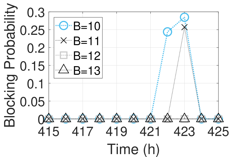
Figure 6: Blocking probability of PAS under PS during the peak hours.

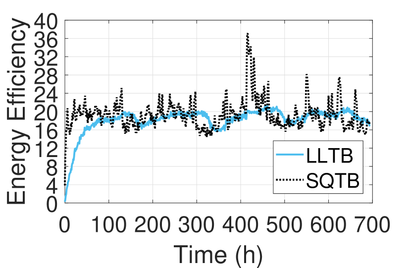
Figure 7: Energy efficiency of PAS with different tie-breaking rules.

Also, we tested the blocking probability of the Google trace-logs used in Figure 5. The system parameters are the same as those for the simulations presented in Figure 5, except that the server buffer sizes are set to $B$ and the $B$ takes different values: $10,11,12,13$. For all the tested buffer sizes, PAS under SRPT and JSQ under both disciplines incur zero blocked jobs based on our simulations; while, as demonstrated in Figure 7, PAS under PS incurs non-negligible blocking probabilities during the peak hours for $B=10,11$ and this reduces to zero for $B\geq 12$. These results strengthen our earlier argument: when the total buffer size of the entire server farm is sufficiently large, the number of blocked jobs becomes negligible even if the heavy traffic condition is satisfied. For a large server farm with 12.5 thousand servers, such as the Google cluster mentioned above, the total buffer size of the entire server farm is already large with relative small $B$.

Moreover, to complete the discussion, in Figure 7, we plot the energy efficiency of PAS under PS with a different tie-breaking rule, but the same settings as the simulations presented in Figure 5. Recall that all our theoretical results apply to any tie-breaking rule, and, as described in Section V, we have just chosen the simplest: when there is more than one server with the highest effective energy efficiency, assign jobs to the server with lowest label. We refer to it as Lowest Label Tie Breaking (LLTB). Alternatively, for multiple servers with the same effective energy efficiency, we could choose the one with the shortest queue; this is referred to as Shortest Queue Tie Breaking (SQTB).

We can see from Figure 7 that LLTB achieves flatter performance, while SQTB is more variable. But in reality there appears to be no general advantage of one over the other. In particular, SQTB outperforms LLTB by around $0.5\%$ with respect to the total energy efficiency and both cases incur no blocked jobs. We then argue that PAS under PS is not very sensitive to different tie-breaking rules. The robustness of PAS to service disciplines demands further exploration involving more comprehensive case studies with real-world trace-logs, but that is outside the scope of this paper.

VII-C Robustness Studies

In practice, job duration times for many online applications have been studied and known to be characterized by heavy tailed distributions [45], which is at odds with our exponential assumption. Hence, it is important to understand the sensitivity of the PAS policy to different job-size distributions. In this context, we consider two heavy-tailed distributions: Pareto with shape parameter $2.001$ (Pareto-F for short) and Pareto with shape parameter $1.98$ (Pareto-INF for short); these are set to have unit mean. Note that Pareto-F and Pareto-INF are Pareto distributions with finite and infinite variance, respectively.

With the same settings as for Section VII-A2, here, we test the energy efficiency of PAS with exponentially, Pareto-F and Pareto-INF distributed job sizes. We also consider a case where the job sizes of different types are distributed differently; this is referred to as the mixed case.

In Figure 8, we demonstrate the robustness of PAS under the PS and SRPT disciplines with respect to different job size distributions. Let $\Gamma^{D}$ represent the energy efficiency of the server farm under PAS with job-size distribution $D$, where $D=$ exponential, mixed, Pareto-F or Pareto-INF.

In Figure 8, we show the cumulative distribution of $(\Gamma^{D}-\Gamma^{\rm exponential})/\Gamma^{\rm exponential}$; that is, the relative difference of energy efficiency with job size distribution $D$ from the one with exponentially distributed job sizes. In Figure 8, this relative difference is within $\pm 1\%$ in all our experiments with randomly generated parameters; while, varies between $-1\%$ and $3\%$ in Figure 8. PAS is resilient to these tested job-sizes distributions under PS and SRPT, although SRPT incurs slightly higher variance than PS.

VIII Conclusions

We have studied the job-assignment problem in a server farm model consisting of a large number of abstracted servers that are possibly diverse in service rates, energy consumption rates, buffer sizes (service capacities) and the ability to serve different jobs. Also, as described in Section III, in this work, the relationship between energy consumption and service rates of servers (abstracted computer components) can be arbitrary, and be determined by the functional features and profiles of servers. By assigning jobs to efficient servers, we aim to balance the job throughput and the power consumption of the system; that is, we aim to maximize the energy efficiency defined as the ratio of long-run average job departure rate to the long-run average energy consumption rate of the entire server farm system.

Following the idea of Whittle relaxation [26], we have proposed the scalable policy, PAS, that prioritizes servers according to only intrinsic attributes and binary state information of different servers among the available ones. PAS accounts for the availability of servers to service different jobs, enabling the applicability of our server farm model to geographically separated computing systems.

To the best of our knowledge, there is no existing work that proposes scalable, infinite horizon policies for such heterogeneous server farms at realistic scales, with a rigorous analysis of performance deviation in terms of energy efficiency.

We have proved that, when job sizes are exponentially distributed, if the blocking probabilities of jobs are always positive or $J=1$, there exists a deviation bound for PAS which is exponentially decreasing in the number of servers in server groups and the average arrival rates of jobs proportionately. This deviation bound indicates the asymptotic optimality of PAS, and, more importantly, significantly improves the asymptotic optimality results: PAS approaches asymptotic optimality very quickly (exponentially) as the server farm size increases. Numerical results illustrate that PAS is already close to OPT for only 100 servers, consistent with our deviation bound. We infer that PAS is nearly optimal for even a relatively small system and any larger one. The robustness of PAS to three different job-size distributions has been tested numerically, with resulting values of energy efficiency in our simulations close to those with exponentially distributed job sizes.

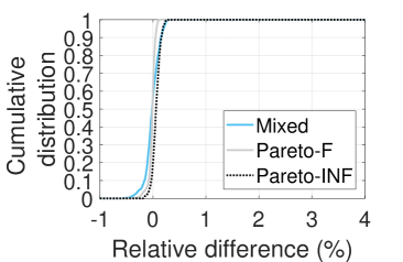
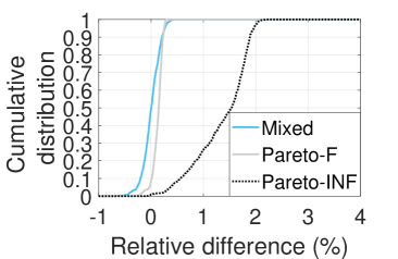
Figure 8: Cumulative distribution of the relative difference of $\Gamma^{D}$ to $\Gamma^{\rm exponential}$ with $D$ = mixed, Pareto-F or Pareto-INF under (a) the PS discipline; and (b) the SRPT discipline.

Appendix A Proof of Proposition 1

Fix a server, $s\in\mathcal{S}$, starting in state $n_{s}\in\mathcal{B}_{k(s)}$, a policy $\phi\in\Phi_{s}$, and a reward rate $f_{k(s)}\in\mathbb{R}^{\mathcal{B}_{k(s)}}$. Write $V^{\phi}_{s}(n_{s},f_{k(s)})$, for the expected value of the cumulative reward for server $s$ that ends when it first enters an absorbing state $n^{0}_{s}\in\mathcal{B}_{k(s)}$. In particular, $V^{\phi}_{s}(n^{0}_{s},f_{k(s)})=0$ for any $\phi\in\Phi_{s}$. We assume, without loss of generality, that $n^{0}_{s}=0$ for all $s\in\mathcal{S}$. Note that such a $V^{\phi}_{s}(n_{s},f_{k(s)})$ is dependent on the values of $\bm{\nu}$ and $\bm{\gamma}$, though we refrain from including them as superscript/subscript to simplify notation. Let $V_{s}(n_{s},f_{k(s)})=\max_{\phi\in\Phi_{s}}V^{\phi}_{s}(n_{s},f_{k(s)})$, $f_{k(s)}\in\mathcal{R}_{k(s)}$, $s\in\mathcal{S}$, $n_{s}\in\mathcal{B}_{k(s)}$.

Now, let $\mathcal{P}^{H}_{s}$, $s\in\mathcal{S}$, represent a process for server $s$ that starts from state $0$ until it reaches state $0$ again, where $\phi\in\Phi_{s}$ is constrained to those policies satisfying $\sum_{j\in\mathcal{J}_{s}}\alpha_{j,s}^{\phi}(0)>0$. From [46, Corollary 6.20 and Theorem 7.5], when the job sizes are exponentially distributed, the process $\mathcal{P}^{H}_{s}$ is a renewal interval of the long-run process, so that the average reward of $\mathcal{P}^{H}_{s}$ equals the long-run average reward of the process for server $s$ under the same policy.

Define, for $s\in\mathcal{S}$, $\phi\in\Phi_{s}$, $n\in\mathcal{B}_{k(s)}$,

$$\tilde{f}_{k(s)}(n)=\left\{\begin{cases}f^{r}_{k(s)}(n)-\sum\limits_{j\in\mathcal{J}_{s}}\nu_{j}\alpha^{\phi}_{j,s}(n),&\text{if }n\in\mathcal{C}_{k(s)},\\ f^{r}_{k(s)}(n)-\sum\limits_{j\in\mathcal{J}_{s}}(\nu_{j}+\eta_{j,s})\alpha^{\phi}_{j,s}(n),&\text{otherwise},\end{cases}\right.$$

where $f^{r}_{k(s)}(n)$ is as defined in (9). Following [46, Theorem 7.6, Theorem 7.7] and [21, Corollary 1], there exists $g\in\mathbb{R}$, with $\tilde{f}^{g}_{k(s)}(n)=\tilde{f}_{k(s)}(n)-g$, $n\in\mathcal{B}_{k(s)}$, such that if policy $\phi^{*}\in\Phi_{s}^{H}$ maximizes the expected cumulative reward of process $\mathcal{P}^{H}_{s}$ with reward rate $\tilde{f}^{g}_{k(s)}(n)$, then $\phi^{*}$ also maximizes the long-run average reward of server $s$ with reward rate $\tilde{f}_{k(s)}(n)$ among all policies in $\Phi_{s}^{H}$. This value of $g$, denoted by $g^{*}_{s}$, is just the maximized long-run average reward.

For $s\in\mathcal{S}$, $j\in\mathcal{J}_{s}$, $n\in\mathcal{C}_{k(s)}$ again for notational simplicity, we write $V^{g}_{s}(n)=V_{s}(n,\tilde{f}^{g}_{k(s)})$ and $r^{g}_{s}(n)=f^{r}_{k(s)}(n)-g$. Note that, in this context, $V^{g}_{s}(0)=V_{s}(0,\tilde{f}^{g}_{k(s)})=0$ since state $0$ is the absorbing state.

Lemma 1.

When the job sizes are exponentially distributed, there exists an policy $\phi^{*}\in\Phi_{s}$, $s\in\mathcal{S}$, that maximizes the objective function given by (16), satisfying: for $n\in\mathcal{C}_{k(s)}$,

$$\alpha^{\phi^{*}}_{j,s}(n)=\left\{\begin{cases}1,&\text{if }\frac{\nu_{j}}{\lambda_{j}}<V_{s}^{g^{*}}(n+1)-V_{s}^{g^{*}}(n),\\ 1\text{ or }0,&\text{if }\frac{\nu_{j}}{\lambda_{j}}=V_{s}^{g^{*}}(n+1)-V_{s}^{g^{*}}(n),\\ 0,&\text{otherwise},\end{cases}\right.$$ (23)

where $g^{*}\coloneqq g^{*}_{s}$ for notational simplicity.

Proof:

We start from (23). Let $\overline{\lambda}_{j,s}(n)=\sum_{j^{\prime}\in\mathcal{J}_{s}:\ j\neq j^{\prime},\ a^{\phi^{*}}_{j^{\prime},s}(n)=1}\lambda_{j^{\prime}}$. Then, from the Bellman equation for Markov Decision Process (MDP), we obtain (23) for $n\in\mathcal{C}_{k(s)}\backslash\{0\}$, which takes values independent of $\overline{\lambda}_{j,s}(n)$ and identically for all $j\in\mathcal{J}_{s}$.

Similarly, the maximization problem based on the Bellman equation for state $n=0$ lead to, for $\overline{\lambda}_{j,s}(0)>0$, equation (23) when $g$ is set to be $g^{*}$. For $\overline{\lambda}_{j,s}(0)=0$, there exists an optimal policy $\phi^{*}\in\Phi_{s}$ with $a^{\phi^{*}}_{j,s}(0)=1$ if and only if $V^{g^{*}}_{s}(1)-(e^{*}\varepsilon_{k(s)}^{0}+\nu_{j}+g^{*})/\lambda_{j}=0$, and $g^{*}\geq-e^{*}\varepsilon_{k(s)}^{0}$, since $g^{*}$ equals the optimal average reward of the same $\mathcal{P}^{H}_{s}$ with reward rate $\tilde{f}_{k(s)}(n)$, $n\in\mathcal{B}_{k(s)}$. These two equations lead to (23) with $n=0$. The lemma is proved. ∎

Lemma 2.

When the job sizes are exponentially distributed, if $\nu=\nu_{j}/\lambda_{j}$ for all $j\in\mathcal{J}$, there exists a policy $\phi^{*}\in\Phi_{s}$ ($s\in\mathcal{S}$) maximizing the objective function given by (16), and satisfying (18) for $s\in\mathcal{S}_{j}$ and $n\in\mathcal{C}_{k(s)}$.

Proof:

From Lemma 1, for any $s\in\mathcal{S}_{j}$, the maximization problem defined in (16) is equivalent to

$$\max\limits_{m\in\mathcal{C}_{k(s)}}\lambda\biggl{(}\frac{\mu_{k(s)}-e^{*}(\varepsilon_{k(s)}-\varepsilon_{k(s)}^{0})}{\mu_{k(s)}}-\nu\biggr{)}\frac{\sum\limits_{n=0}^{m}\left(\frac{\lambda}{\mu_{k(s)}}\right)^{n}}{\sum\limits_{n=0}^{m+1}\left(\frac{\lambda}{\mu_{k(s)}}\right)^{n}},$$

where $\lambda=\sum_{j\in\mathcal{J}_{s}}\lambda_{j}$. Solving it, we obtain (18). ∎

We now give the proof of Proposition 1.

Proof:

The proof consists of two parts:

1. we construct a set of $\bm{\nu}$, $\bm{\gamma}$, $\varphi_{j}\in\overline{\Phi}_{j}$, $j\in\mathcal{J}$, and $\phi^{*}_{s}\in\Phi_{s}$, $s\in\mathcal{S}$, where $\phi^{*}_{s}$ and $\varphi_{j}$ maximize the objective functions defined in (16) and (17), respectively;

2. and we prove that a policy consisting of such $\varphi_{j}$, $j\in\mathcal{J}$, and $\phi^{*}_{s}$, $s\in\mathcal{S}$, maximizes the relaxed problem defined by (10), (11), (13)-(14).

We firstly discuss the case where Condition 1 holds. Let

1. $\nu_{j}/\lambda_{j}=\nu$ and $\nu=\min\Bigl{\{}0,\min\limits_{s\in\mathcal{S}_{j}}\bigl{(}1-e^{*}\frac{\varepsilon_{k(s)}-\varepsilon_{k(s)}^{0}}{\mu_{k(s)}}\bigr{)}\Bigr{\}}$;

2. $\gamma_{j}=-\lambda_{j}\nu$, $j\in\mathcal{J}$.

From Lemma 2, there is an optimal policy $\phi^{*}_{s}\in\Phi_{s}$ that maximizes the problem defined in (16), satisfying $\alpha^{\phi^{*}_{s}}_{j,s}(n)=1$ for all $j\in\mathcal{J}$, $s\in\mathcal{S}_{j}$, $n\in\mathcal{C}_{k(s)}$. There is also a policy $\varphi_{j}\in\overline{\Phi}_{j}$, $j\in\mathcal{J}$, for the maximization problem defined by (17), satisfying $\overline{a}^{\varphi_{j}}_{j}=1-A_{j}$ and $\alpha^{\varphi_{j}}_{j}=1-A_{j}$. Note that $1-A_{j}\in[0,1)$ under Condition 1.

Therefore, Constraints (11), (13) and (14) are satisfied with equality: the complementary slackness condition for the dual and primal problems is satisfied. The optimal solution $\phi^{*}$ determined by $\phi^{*}_{s}$ ($s\in\mathcal{S}$) and $\varphi_{j}$ ($j\in\mathcal{J}$) that maximizes the Lagrangian problem defined in (15) will also maximize the primal problem defined by (10), (11), (13)-(14).

We now consider the case where $J=1$ and denote the only $j$ in $\mathcal{J}$ by $j^{*}$. The proposition can be proved along the same lines as the $J>1$ case if $A_{j^{*}}\leq 1$. If $A_{j^{*}}>1$, then let $\gamma_{j^{*}}=\max\left\{0,-\nu_{j^{*}}\right\}$. From Lemma 2, there is an optimal policy $\phi^{*}_{s}\in\Phi_{s}$ that maximizes the problem defined in (16), satisfying (18) for $j=j^{*}$, $s\in\mathcal{S}_{j^{*}}$ and $n\in\mathcal{C}_{k(s)}$. Since $A_{j^{*}}>1$, there exists a $\nu_{j^{*}}\geq\min_{s\in\mathcal{S}_{j^{*}}}\lambda_{j^{*}}(1-e^{*}(\varepsilon_{k(s)}-\varepsilon_{k(s)}^{0})/\mu_{k(s)})$, such that $\sum_{s\in\mathcal{S}_{j^{*}}}\sum_{n\in\mathcal{B}_{k(s)}}\pi^{\phi^{*}_{s}}_{s}(n)\alpha^{\phi^{*}_{s}}_{s}(n)=1$. Note that $\phi^{*}_{s}$ is dependent on $\nu_{j^{*}}$.

On the other hand, the setting of $\gamma_{j^{*}}$ guarantees that there is a policy $\varphi\in\overline{\Phi}_{j^{*}}$ maximizing the objective function defined by (17), and satisfying $\alpha^{\varphi}_{j^{*}}=0$ and $\Theta(\overline{a}^{\varphi}_{j^{*}})=0=\Theta(1-A_{j^{*}})$, e.g., equations (11) and (13) achieve equality. That is, such a $\nu_{j^{*}}$, $\gamma_{j^{*}}$, $\phi^{*}_{s}\in\Phi_{s}$, $s\in\mathcal{S}_{j^{*}}$ and $\varphi\in\overline{\Phi}_{j^{*}}$, make the complementary slackness condition satisfied. ∎

Appendix B Proof of Proposition 2

Consider $J+|\mathcal{S}|$ sequences of positive reals $t^{h}_{s,m}$, $m=1,2,\ldots$, for $s=1,2,\ldots,J+|\mathcal{S}|$, where $h\in\mathbb{N}_{+}$ is the scaling parameter. We define $t^{h}_{s,m}$ for $s=1,2,\ldots,J$ as time of the $m$th arrival of jobs of type $s$, and define $t^{h}_{s,m}$ for $s=J+1,J+2,\ldots,J+|\mathcal{S}|$ to be the time of the $m$th potential departure of jobs on server labeled by $s-J$. Define $t^{h}_{s,0}=0$ for any $s=1,2,\ldots,J+|\mathcal{S}|$. For our network system, the inter-arrival and inter-departure times are positive with probability $1$ and, also with probability $1$, no two events occur at the same time. Let $\tau(t)$ represent the latest event, either arrival or potential departure, that happens before time $t$. We define a random vector $\bm{\xi}^{h}_{t}$, for $s=1,2,\ldots,|\mathcal{S}|+J$ and $t\geq 0$: if $\tau(t^{h}_{s,m})\leq t<t^{h}_{s,m^{*}}$ where the $m^{*}$ satisfies $t^{h}_{s,m^{*}-1}\leq t<t^{h}_{s,m^{*}}$, then $\xi^{h}_{s,t}=1/(t^{h}_{s,m^{*}}-\tau(t^{h}_{s,m^{*}}))$; otherwise, $\xi^{h}_{s,t}=0$. The sample paths of $\bm{\xi}^{h}_{t}$ are almost surely continuous in $t\geq 0$, except for a finite number of discontinuities of the first kind in a bounded period of $t>0$. Let $\Lambda_{j,i}(\bm{x})=u^{PAS,h}_{j,i}(\frac{\bm{x}}{hS_{0}})z_{i}hS_{0}$, which is independent from $h$ from the definition of $u^{PAS,h}_{j,i}(\cdot)$. We define a function, $Q^{h}(i,i^{\prime},\bm{x},\bm{\xi}^{h})$, for $h\in\mathbb{N}^{+}$, $n_{i},n_{i^{\prime}}\in\mathcal{B}_{k}$, $k\in\mathcal{K}\cup\{0\}$, $\bm{x}\in\mathbb{R}^{I}$, $\bm{\xi}^{h}\in\mathbb{R}^{hS_{0}+J}$, by: if $k_{i}=k_{i^{\prime}}$ and $i^{\prime}=i+1$,

$$Q^{h}(i,i^{\prime},\bm{x},\bm{\xi}^{h})=\sum_{j\in\mathcal{J}_{k_{i}}}\left[\Lambda_{j,i}(\bm{x})\ +f^{0,h}_{i,a,j}(\bm{x})\right]\xi^{h}_{j};\vspace{-0.2cm}$$

if $k_{i}=k_{i^{\prime}}$ and $i^{\prime}=i-1$,

$$Q^{h}(i,i^{\prime},\bm{x},\bm{\xi}^{h})=\sum\limits_{m=\lceil x^{-}_{i-1}\rceil+1}^{\lceil x^{-}_{i}\rceil}\xi^{h}_{m+J}+\sum\limits_{m=1}^{hS_{0}}f^{h}_{i,a,m}(\bm{x})\xi^{h}_{m+J};\vspace{-0.2cm}$$

otherwise, $Q^{h}(i,i^{\prime},\bm{x},\bm{\xi}^{h})=0$; where $\mathcal{J}_{k}=\{j\in\mathcal{J}|\ k\in\mathcal{K}_{j}\}$, $k\in\mathcal{K}$, $x^{-}_{i}=\sum_{m=1}^{i}x_{m}$ with $x^{-}_{0}=0$, and $\bm{f}^{0,h}_{i,a}(\bm{x})\in\mathbb{R}^{J}$ and $\bm{f}^{h}_{i,a}(\bm{x})\in\mathbb{R}^{hS_{0}}$ with $0<a<1$ are appropriate functions as described in [38] such that $Q^{h}$ is Lipschitz continuous in $\bm{x}$. For the special case $h=1$ and for any given $0<a<1$, $Q^{\phi,1}(i,i^{\prime},\bm{x},\bm{\xi}^{1})$ satisfies a Lipschitz condition over $\bm{x}\in\mathbb{R}^{I}$ and $\bm{\xi}^{1}\in\mathbb{R}^{S_{0}+J}$. For $0<a<1$ and $\epsilon>0$, define

$$\dot{X}_{t,i}^{\epsilon}\coloneqq\sum\limits_{i^{\prime}=1}^{I}Q^{1}(i^{\prime},i,\bm{X}^{\epsilon}_{t},\bm{\xi}_{t/\epsilon}^{1})-Q^{1}(i,i^{\prime},\bm{X}^{\epsilon}_{t},\bm{\xi}_{t/\epsilon}^{1})\\ =(\overline{\bm{q}}_{i}(\bm{X}^{\epsilon}_{t}),\bm{\xi}^{1}_{t/\epsilon}),$$

where $\overline{\bm{q}}_{i}(\bm{x})$ is a vector of length $S_{0}+J$ dependent on $\bm{x}$ and $(\cdot,\cdot)$ represents inner product of vectors. It follows that $\dot{\bm{X}}_{t}^{\epsilon}$ satisfies a Lipschitz condition over $\bm{X}^{\epsilon}_{t}$ and $\bm{\xi}^{1}_{t/\epsilon}$. Let

$$b(\bm{x},\bm{\xi})\coloneqq((\overline{\bm{q}}_{i}(\bm{x}),\bm{\xi}):i=1,2,\ldots,I)\coloneqq\overline{\mathcal{Q}}(\bm{x})\bm{\xi},$$

where where $\overline{Q}(\bm{x})$ is a $I\times(S_{0}+J)$ matrix. For any $\bm{x}\in\mathbb{R}^{I}$, $\delta>0$, there exists $\overline{b}(\bm{x})$ satisfying

$$\lim\limits_{T\rightarrow+\infty}\mathbb{P}\biggl{\{}\Bigl{\lVert}\frac{1}{T}\int_{t}^{t+T}b^{\phi}(\bm{x},\bm{\xi}^{1}_{s})ds-\overline{b}(\bm{x})\Bigr{\rVert}>\delta\biggr{\}}=0,$$ (24)

uniformly in $t>0$. Let $\overline{\bm{x}}(t)$ be the solution of $\dot{\overline{\bm{x}}}(t)=\overline{b}(\overline{\bm{x}}(t))$ and $\overline{\bm{x}}(0)=\bm{X}^{\epsilon}_{0}=\bm{x}_{0}$. Define, for $Y=S_{0}+J$, the random variables $\bm{\xi}^{1}_{t}$ and vectors $\bm{\alpha}_{t}\in\mathbb{R}^{Y}$,

$$\int_{0}^{T}H_{\xi}(\bm{\alpha}_{t})d\ t=\lim\limits_{\varepsilon\to 0}\varepsilon\ln\mathbb{E}\ \exp\Bigl{\{}\frac{1}{\varepsilon}\int_{0}^{T}(\bm{\alpha}_{t},\bm{\xi}^{1}_{t/\varepsilon})dt\Bigr{\}}.$$ (25)

We discuss the existence of $H_{\xi}(\cdot)$ satisfying (25) next. Let $\bm{\Upsilon}_{T}=\int_{0}^{T}\bm{\xi}^{1}_{t}dt,$ which is a Poisson distributed random vector. Writing $\bm{\alpha}=(\alpha_{1},\alpha_{2},\ldots,\alpha_{Y})$, we obtain

$$H_{\xi}(\bm{\alpha})=\sum_{j=1}^{J}\lambda_{j}(e^{\alpha_{j}}-1)+\sum_{s\in\mathcal{S}}\mu_{k(s)}(e^{\alpha_{J+s}}-1).$$ (26)

It follows that $H_{\xi}(\bm{\alpha})$ satisfying (26) is bounded for any bounded $\bm{\alpha}$, so that the functional $H_{\xi}(\bm{\alpha}_{t})$ satisfying (25) also exists for any continuous $\bm{\alpha}_{t}$ on $0\leq t\leq T$. For a vector $\bm{U}\in(\mathbb{R}^{+})^{Y}$, define a function $\mathcal{T}^{\bm{U}}$ for $i=1,2,\ldots,Y$ and $\bm{x}\in\mathbb{R}^{Y}$: if $0\leq x_{i}\leq U_{i}$, $\mathcal{T}^{\bm{U}}_{i}(\bm{x})=x_{i}$; if $x_{i}>U_{i}$, $\mathcal{T}^{\bm{U}}_{i}(\bm{x})=U_{i}$; otherwise, $\mathcal{T}^{\bm{U}}_{i}(\bm{x})=0$. For $\tilde{\bm{\alpha}},\bm{x}\in\mathbb{R}^{I}$, define

$$H(\bm{x},\tilde{\bm{\alpha}})=\lim\limits_{T\rightarrow+\infty}\frac{1}{T}\ln\mathbb{E}\exp\Bigl{\{}\int\limits_{0}^{T}(\tilde{\bm{\alpha}},\tilde{b}^{\bm{U}}(\bm{x},\bm{\xi}^{1}_{t}))dt\Bigr{\}}\vspace{-0.2cm}$$ (27)

where $\tilde{b}^{\bm{U}}(\bm{x},\bm{y})\coloneqq b(\bm{x},\mathcal{T}^{\bm{U}}(\bm{y}))=\overline{\mathcal{Q}}(\bm{x})\mathcal{T}^{\bm{U}}(\bm{y}).$ Here, since $b(\cdot,\cdot)$ is Lipschitz continuous in both arguments, all of the elements of $\bm{U}$ are finite and positive, and for $\overline{\mathcal{Q}}(\cdot)=(q_{i,j})$, $|q_{i,j}|<+\infty$ for all $i=1,2,\ldots,I$ and $j=1,2,\ldots,Y$, we obtain that $\tilde{b}^{\bm{U}}(\cdot,\cdot)$ is bounded and Lipschitz continuous in both arguments. From [47, Lemma 4.1, Chapter 7], $H(\bm{x},\bm{y})$ is jointly continuous in both arguments and convex in the second argument.

We obtain from (27), for any $\tilde{\bm{\alpha}},\bm{x}\in\mathbb{R}^{I}$, $|H(\bm{x},\tilde{\bm{\alpha}})|\leq H_{\xi}(\mathcal{A}(\tilde{\bm{\alpha}}\overline{\mathcal{Q}}(\bm{x})))$, where $\mathcal{A}(\bm{x})$ takes absolute values of all $\bm{x}$’s elements. Recall that $\overline{\mathcal{Q}}(\bm{x})$, $\bm{x}\in\mathbb{R}^{I}$, is Lipschitz continuous on $\bm{x}$. For any compact set $\mathcal{A}^{c}\subset\mathbb{R}^{I}$ and $\tilde{\bm{\alpha}}\in\mathcal{A}^{c}$, $H(\bm{x},\tilde{\bm{\alpha}})$ obtained from (27) is bounded and because of its joint continuity, is Riemann integrable. Hence, the $H(\bm{x},\tilde{\bm{\alpha}})$ defined in (27) satisfies

$$\int\limits_{0}^{T}H(\bm{x}_{t},\tilde{\bm{\alpha}}_{t})dt=\lim\limits_{\varepsilon\to 0}\varepsilon\ln\mathbb{E}\text{exp}\Bigl{\{}\frac{1}{\varepsilon}\int\limits_{0}^{T}(\tilde{\bm{\alpha}}_{t},\bm{\xi}^{1}_{t/\varepsilon})dt\Bigr{\}}.\vspace{-0.2cm}$$ (28)

Now we consider the Legendre transform of $H(\bm{x},\tilde{\bm{\alpha}})$:

$$L(\bm{x},\bm{\beta})=\sup_{\tilde{\bm{\alpha}}\in\mathbb{R}^{I}}\left[(\tilde{\bm{\alpha}},\bm{\beta})-H(\bm{x},\tilde{\bm{\alpha}})\right].$$ (29)

$L(\bm{x},\bm{\beta})$ is strictly convex in the second argument if $H(\bm{x},\tilde{\bm{\alpha}})$ is strictly convex in the second argument. Let $\tilde{\bm{\alpha}}=\bm{0}$, $(\tilde{\bm{\alpha}},\bm{\beta})-H(\bm{x},\tilde{\bm{\alpha}})=0$, so that $L(\bm{x},\bm{\beta})$ is always non-negative.

Lemma 3.

If $L(\bm{\varphi},\bm{\beta})$ is strictly convex in the second argument, then $L(\bm{\varphi},\bm{\beta})=0$ if and only if $\bm{\beta}=\mathbb{E}\tilde{b}^{\bm{U}}(\bm{\varphi},\bm{\xi}^{1}_{t})$.

Proof:

The $L(\bm{\varphi},\bm{\beta})=0$ when $\bm{\beta}=\mathbb{E}\tilde{b}^{\bm{U}}(\bm{\varphi},\bm{\xi}^{1}_{t})$, [47, Chapter 7, Section 4]. Together with non-negativity and strict convexity of $L(\bm{\varphi},\bm{\beta})$, for a given $\bm{\varphi}\in\mathbb{R}^{I}$, $L(\bm{\varphi},\bm{\beta})=0$ if and only if $\bm{\beta}=\mathbb{E}\tilde{b}^{\bm{U}}(\bm{\varphi},\bm{\xi}^{1}_{t})$. ∎

The second derivative $\partial^{2}H/\partial\tilde{\bm{\alpha}}^{2}$ exists and is continuous in $\bm{U}$, and as $\bm{U}\to\bm{\infty}$, it converges point-wisely to $\partial^{2}H_{\xi}(\tilde{\bm{\alpha}}\overline{Q}(\bm{x}))/\partial\tilde{\bm{\alpha}}^{2}$; the function $H_{\xi}(\tilde{\bm{\alpha}}\overline{Q}(\bm{x}))$ is strictly convex in $\tilde{\bm{\alpha}}$ by (26) and the second derivative in $\tilde{\bm{\alpha}}$ exists. Thus, for sufficiently large $\bm{U}$, $L(\bm{\varphi},\bm{\beta})$ is always strictly convex in the second argument.

Proof:

Let $S_{0,T}(\varphi)=\int_{0}^{T}L(\bm{\varphi}_{t},\dot{\bm{\varphi}}_{t})d\ t$, where $\varphi$ denotes a trajectory $\bm{\varphi}_{t}\in\mathbb{R}^{I}$ ($0\leq t\leq T$), and let $C_{0,T}$ represent the compact set of all such trajectories with $\bm{\varphi}_{0}=\bm{x}_{0}\in\mathbb{R}^{I}$. Define a closed set $A(\bm{U},\delta)\coloneqq\{\varphi\in C_{0,T}|\lVert\varphi_{t}-\tilde{\bm{x}}^{\bm{U}}_{t}\rVert\geq\delta\}$ where $\tilde{\bm{x}}^{\bm{U}}_{t}$ is the solution of $\dot{\tilde{\bm{x}}}^{\bm{U}}_{t}=\mathbb{E}\tilde{b}^{\bm{U}}(\bm{\varphi},\bm{\xi}^{1}_{t})$ with $\tilde{\bm{x}}^{\bm{U}}_{0}=\bm{x}_{0}$. From [47, Theorem 4.1 in Chapter 7 & Theorem 3.3 in Chapter 3], for any $\bm{U}\in(\mathbb{R}^{+})^{Y}$ and $\delta>0$,

$$\overline{\lim\limits_{\epsilon\to 0}}~{}\epsilon\ln\mathbb{P}\Bigl{\{}\sup\limits_{0\leq t\leq T}\bigl{\lVert}\tilde{\bm{X}}^{\bm{U},\epsilon}_{t}-\tilde{\bm{x}}^{\bm{U}}_{t}\bigr{\rVert}>\delta\Bigr{\}}\leq-\inf_{\varphi\in A(\bm{U},\delta)}S_{0,T}(\varphi),$$

where $\tilde{\bm{X}}^{\bm{U},\epsilon}_{t}$ is the solution of

$$\dot{\tilde{\bm{X}}}_{t}^{\bm{U},\epsilon}=\tilde{b}^{\bm{U}}(\tilde{\bm{X}}_{t}^{\bm{U},\epsilon},\bm{\xi}^{1}_{t})),~{}\tilde{\bm{X}}_{0}^{\bm{U},\epsilon}=\bm{x}_{0}.\vspace{-0.3cm}$$

Also, because

$$\lim_{\bm{U}\rightarrow\bm{\infty}}\tilde{\bm{x}}^{\bm{U}}_{t}=\overline{\bm{x}}(t)~{}\text{and}~{}\lim_{\bm{U}\rightarrow\bm{\infty}}\tilde{\bm{X}}^{\bm{U},\epsilon}_{t}=\bm{X}^{\epsilon}_{t},\vspace{-0.2cm}$$

by Lemma 3, we obtain, for any $\delta>0$, there exist $s>0$ and $\epsilon_{0}>0$ such that, for all positive $\epsilon<\epsilon_{0}$,

$$\mathbb{P}\Bigl{\{}\sup\limits_{0\leq t\leq T}\lVert\bm{X}^{\epsilon}_{t}-\overline{\bm{x}}(t)\rVert>\delta\Bigr{\}}\leq e^{-\frac{s}{\epsilon}}.\vspace{-0.2cm}$$ (30)

Recall that functions $Q^{h}$ and $b$ are depenedent on a parameter $a\in(0,1)$. Equation (30) holds for any given $a$. Because of the Lipschitz behavior of $\dot{\bm{X}}^{\epsilon}_{t}$ and $\dot{\overline{\bm{x}}}(t)$ on $0<a<1$, $\lim_{a\to 0}d\dot{\bm{X}}^{\epsilon}_{t}/da=0$ and $\lim_{a\to 0}d\dot{\overline{\bm{x}}}(t)/da=0$, Equation (30) also holds in the limiting case $a\to 0$. By slightly abusing notation, in the following, we still use $Q^{h}$, $b$ and $\bar{\bm{x}}(t)$ to represent $\lim_{a\to 0}Q^{h}$, $\lim_{a\to 0}b$ and $\lim_{a\to 0}\bar{\bm{x}}(t)$.

Along similar lines to [21], we interpret the scalar $\epsilon$ and the scaling effects in another way. For $\bm{x}\in\mathbb{R}^{I}$ and $\bm{\xi}^{h}\in\mathbb{R}^{hS_{0}+J}$, define

$$b^{h}(\bm{x},\bm{\xi}^{h})\coloneqq\sum_{i^{\prime}=1}^{I}Q^{h}(i^{\prime},i,\bm{x},\bm{\xi}^{h})-Q^{h}(i,i^{\prime},\bm{x},\bm{\xi}^{h}).\vspace{-0.2cm}$$

If we set $\epsilon=1/h$, then following the same technique as [21], for any $\bm{x}\in\mathbb{R}^{I}$, $h\in\mathbb{N}^{+}$ and $T>0$, we observe that $\int_{0}^{T}b(\bm{x},\xi^{1}_{t/\epsilon})d\ t$ and $\int_{0}^{T}(b^{h}(h\bm{x},\xi^{h}_{t})/h)d\ t$ are identically distributed. Define $\bm{Z}^{\epsilon}_{0}=\bm{Z}^{h}_{0}=\bm{x}_{0}/S_{0}=\bm{z}^{0}$, and

$$\dot{\bm{Z}}^{h}_{t}=\frac{b^{h}(hS_{0}\bm{Z}^{h}_{t},\bm{\xi}^{h}_{t})}{hS_{0}}\text{ and }\dot{\bm{Z}}^{\epsilon}_{t}=\frac{b(S_{0}\bm{Z}^{\epsilon}_{t},\bm{\xi}^{1}_{t/\epsilon})}{S_{0}}.$$

From (30), for any $T>0$, $\delta>0$, there exist positive $s$ and $H$ such that, for all $h>H$,

$$\mathbb{P}\biggl{\{}\sup\limits_{0\leq t\leq T}\Bigl{\lVert}\bm{Z}^{h}_{t}-\overline{\bm{x}}(t)/S_{0}\Bigr{\rVert}>\delta\biggr{\}}\leq e^{-sh}.$$ (31)

Effectively then, scaling time by $\epsilon=\frac{1}{h}$ is equivalent to scaling system size by $h$. From (31), Corollary 1 and [38, Lemma 3], for any $T>0$, $\delta>0$, there exist $s>0$ and $H>0$ such that for any $h>H$, (22) holds. ∎

Appendix C Settings for Simulations in Figure 5

Define Case I as a system with same settings as in the simulations for Figure 1, except for the following parameters:

• $\mu_{1}=8.06114$, $\varepsilon_{1}^{0}=0.80611$, $\varepsilon_{1}=8.06114$;

• $\mu_{2}=4.05127$, $\varepsilon_{2}^{0}=0.94774$, $\varepsilon_{2}=4.73868$;

• $\mu_{3}=3.70788$, $\varepsilon_{3}^{0}=2.21086$, $\varepsilon_{3}=7.36952$;

• $\mu_{4}=2.88018$, $\varepsilon_{4}^{=}4.40851$, $\varepsilon_{4}=11.02129$;

• $\mu_{5}=2.44950$, $\varepsilon_{5}^{0}=8.79314$, $\varepsilon_{5}=17.58627$;

• and $\lambda_{1}=6.30639$, $\mathcal{K}_{1}=\{1,5\}$.

Define Case II as a system with same settings as in the simulations for Figure 1, except for the following parameters:

• $\mu_{1}=7.74574$, $\varepsilon_{1}^{0}=0.77457$, $\varepsilon_{1}=7.74574$;

• $\mu_{2}=7.46818$, $\varepsilon_{2}^{0}=1.77913$, $\varepsilon_{2}=8.89565$;

• $\mu_{3}=6.32019$, $\varepsilon_{3}^{0}=2.65737$, $\varepsilon_{3}=8.85791$;

• $\mu_{4}=4.66817$, $\varepsilon_{4}^{0}=3.27786$, $\varepsilon_{4}=8.19465$;

• $\mu_{5}=4.62779$, $\varepsilon_{5}^{0}=4.82040$, $\varepsilon_{5}=9.64079$;

• $\lambda_{1}=11.04970$, $\mathcal{K}_{1}=\{2,3,5\}$;

• $\lambda_{2}=8.27302$, $\mathcal{K}_{2}=\{2,3\}$;

• $\lambda_{3}=11.04970$, $\mathcal{K}_{3}=\{2,3,5\}$.

Note that both examples are taking instances of the randomly generated system in simulations in Sections VII-A1 and VII-A2.

Appendix D Settings for Simulations in Section VII-B

Consider ten server groups with the following parameters:

• $\mu_{1}=2.42523$, $\varepsilon_{1}^{0}=0.06548$, $\varepsilon_{1}=0.242523$;

• $\mu_{2}=2.41588$, $\varepsilon_{2}^{0}=0.04974$, $\varepsilon_{2}=0.207254$;

• $\mu_{3}=2.38966$, $\varepsilon_{3}^{0}=0.04279$, $\varepsilon_{3}=0.20377$;

• $\mu_{4}=2.22434$, $\varepsilon_{4}^{0}=0.02630$, $\varepsilon_{4}=0.14613$;

• $\mu_{5}=1.75822$, $\varepsilon_{5}^{0}=0.07228$, $\varepsilon_{5}=0.60241$;

• $\mathcal{K}_{1}=\{1,5,6,10\}$, $B_{1}=20$;

• $\mathcal{K}_{2}=\{1,2,3,4,5,7,8,9\}$, $B_{2}=20$;

• $\mathcal{K}_{3}=\{1,6,7,10\}$, $B_{3}=20$; and $\mathcal{K}_{4}=\{2\}$, $B_{4}=20$.

Note that all the numbers are generated by a pseudo-random number generator, and the unit of service rates $\mu_{k}$ is $10^{-4}s^{-1}$: the number of processed jobs per second. The values of $\mu_{k}$ are normalized to be sufficiently small that we can observe a positive number of blocked jobs in Figure 7, and the heavy traffic condition can be achieved during the peak hours as presented in Section VII-B.

References

- [1] Emerson Network Power, “State of the data center 2011,” 2011. [Online]. Available: http://www.emersonnetworkpower.com/en-US/Solutions/ infographics/Pages/2011DataCenterState.aspx
- [2] Natural Resources Defense Council, “America’s data centers consuming massive and growing amounts of electricity,” Aug. 2014. [Online]. Available: http://www.nrdc.org/media/2014/140826.asp
- [3] D. Kliazovich, P. Bouvry, F. Granelli, and N. L. S. da Fonseca, “Energy consumption optimization in cloud data centers,” in Cloud Services, Networking, and Management, N. L. S. da Fonseca and R. Boutaba, Eds. John Wiley & Sons, Inc, Apr. 2015, pp. 191–215. [Online]. Available: http://dx.doi.org/10.1002/9781119042655.ch8
- [4] S. Albers, F. Müller, and S. Schmelzer, “Speed scaling on parallel processors,” Algorithmica, vol. 68, no. 2, pp. 404–425, Feb. 2014.
- [5] J. Lenhardt, K. Chen, and W. Schiffmann, “Energy-efficient web server load balancing,” IEEE Syst. J., vol. 11, no. 2, pp. 878–888, Jun. 2017.
- [6] M. Lin, A. Wierman, L. L. H. Andrew, and E. Thereska, “Dynamic right-sizing for power-proportional data centers,” IEEE/ACM Trans. Netw., vol. 21, no. 5, pp. 1378–1391, Oct. 2013.
- [7] Y. Yao, L. Huang, A. B. Sharma, L. Golubchik, and M. J. Neely, “Power cost reduction in distributed data centers: A two-time-scale approach for delay tolerant workloads,” IEEE Trans. Parallel Distrib. Syst., vol. 25, no. 1, pp. 200–211, Jan. 2014.
- [8] E. Hyyti, R. Righter, and S. Aalto, “Task assignment in a heterogeneous server farm with switching delays and general energy-aware cost structure,” Performance Evaluation, vol. 75-76, pp. 17–35, 2014.
- [9] M. E. Gebrehiwot, S. Aalto, and P. Lassila, “Near-optimal policies for energy-aware task assignment in server farms,” in Proc. CCGrid 2017. Madrid, Spain: IEEE Press, May 2017, pp. 1017–1026.
- [10] T. Lin, T. Alpcan, and K. Hinton, “A game-theoretic analysis of energy efficiency and performance for cloud computing in communication networks,” IEEE Syst. J., vol. 11, no. 2, pp. 649–660, Jun. 2017.
- [11] W. Shi, C. Wu, and Z. Li, “An online auction mechanism for dynamic virtual cluster provisioning in geo-distributed clouds,” IEEE Trans. Parallel Distrib. Syst., vol. 28, no. 3, pp. 677–688, Mar. 2017.
- [12] W. Q. M. Guo, A. Wadhawan, L. Huang, and J. T. Dudziak, “Server farm management,” Patent 8,626,897, Jan., 2014.
- [13] A. Hameed, A. Khoshkbarforoushha, R. Ranjan, P. P. Jayaraman, J. Kolodziej, P. Balaji, S. Zeadally, Q. M. Malluhi, N. Tziritas, A. Vishnu, S. U. Khan, and A. Zomaya, “A survey and taxonomy on energy efficient resource allocation techniques for cloud computing systems,” Computing, vol. 98, no. 7, pp. 751–774, Jun. 2016.
- [14] A. Gandhi and M. Harchol-Balter, “How data center size impacts the effectiveness of dynamic power management,” in Proc. 2011 49th Annual Allerton Conference on Communication, Control, and Computing (Allerton). Monticello, IL, USA: IEEE, Sep. 2011, pp. 1164–1169.
- [15] T. Lu, M. Chen, and L. L. H. Andrew, “Simple and effective dynamic provisioning for power-proportional data centers,” IEEE Trans. Parallel Distrib. Syst., vol. 24, no. 6, pp. 1161–1171, Apr. 2013.
- [16] Z. Rosberg, Y. Peng, J. Fu, J. Guo, E. W. M. Wong, and M. Zukerman, “Insensitive job assignment with throughput and energy criteria for processor-sharing server farms,” IEEE/ACM Trans. Netw., vol. 22, no. 4, pp. 1257–1270, Aug. 2014.
- [17] J. Fu, J. Guo, E. W. M. Wong, and M. Zukerman, “Energy-efficient heuristics for insensitive job assignment in processor-sharing server farms,” IEEE J. Sel. Areas Commun., vol. 33, no. 12, pp. 2878–2891, Dec. 2015.
- [18] L. A. Barroso and U. Holzle, “The case for energy-proportional computing,” Computer, vol. 40, no. 12, pp. 33–37, Dec. 2007.
- [19] M. Chowdhury, M. R. Rahman, and R. Boutaba, “Vineyard: Virtual network embedding algorithms with coordinated node and link mapping,” IEEE/ACM Trans. Netw., vol. 20, no. 1, pp. 206–219, Feb. 2012.
- [20] F. Esposito, D. Di Paola, and I. Matta, “On distributed virtual network embedding with guarantees,” IEEE/ACM Trans. Netw., vol. 24, no. 1, pp. 569–582, Feb. 2016.
- [21] J. Fu, B. Moran, J. Guo, E. W. M. Wong, and M. Zukerman, “Asymptotically optimal job assignment for energy-efficient processor-sharing server farms,” IEEE J. Sel. Areas Commun., 2016.
- [22] U. Ayesta, M. Erausquin, M. Jonckheere, and I. M. Verloop, “Scheduling in a random environment: stability and asymptotic optimality,” IEEE/ACM Trans. Netw., vol. 21, no. 1, pp. 258–271, Feb. 2013.
- [23] I. M. Verloop, “Asymptotically optimal priority policies for indexable and non-indexable restless bandits,” Ann. Appl. Probab., vol. 26, no. 4, pp. 1947–1995, Aug. 2016.
- [24] V. Gupta, “Stochastic models and analysis for resource management in server farms,” Ph.D. dissertation, School of Computer Science, Carnegie Mellon University, 2011.
- [25] Y. Sakuma, “Asymptotic behavior for MAP/PH/c queue with shortest queue discipline and jockeying,” Oper. Res. Lett., vol. 38, no. 1, pp. 7–10, Jan. 2010.
- [26] P. Whittle, “Restless bandits: Activity allocation in a changing world,” J. Appl. Probab., vol. 25, pp. 287–298, 1988.
- [27] C. H. Papadimitriou and J. N. Tsitsiklis, “The complexity of optimal queuing network control,” Math. Oper. Res., vol. 24, no. 2, pp. 293–305, May 1999.
- [28] R. R. Weber and G. Weiss, “On an index policy for restless bandits,” J. Appl. Probab., no. 3, pp. 637–648, Sep. 1990.
- [29] J. Niño-Mora, “Restless bandits, partial conservation laws and indexability,” Advances in Applied Probability, vol. 33, no. 1, pp. 76–98, 2001.
- [30] J. Niño-Mora, “Dynamic allocation indices for restless projects and queueing admission control: a polyhedral approach,” Mathematical programming, vol. 93, no. 3, pp. 361–413, 2002.
- [31] J. Niño-Mora, “Dynamic priority allocation via restless bandit marginal productivity indices,” TOP, vol. 15, no. 2, pp. 161–198, Sep. 2007.
- [32] X. Wei and M. J. Neely, “Data center server provision: Distributed asynchronous control for coupled renewal systems,” IEEE/ACM Transactions on Networking, vol. 25, no. 4, pp. 2180 – 2194, Aug. 2017.
- [33] M. Pore, Z. Abbasi, S. K. S. Gupta, and G. Varsamopoulos, “Techniques to achieve energy proportionality in data centers: A survey,” in Handbook on Data Centers. Springer, Mar. 2015, pp. 109–162.
- [34] K. Li, “Quantitative modeling and analytical calculation of elasticity in cloud computing,” IEEE Transactions on Cloud Computing, 2017.
- [35] S. Sebastio, M. Amoretti, A. L. Lafuente, and A. Scala, “A holistic approach for collaborative workload execution in volunteer clouds,” ACM Transactions on Modeling and Computer Simulation (TOMACS), vol. 28, no. 2, p. 14, 2018.
- [36] M. Guo, Q. Guan, and W. Ke, “Optimal scheduling of VMs in queueing cloud computing systems with a heterogeneous workload,” IEEE Access, vol. 6, pp. 15 178–15 191, 2018.
- [37] C. Reiss, A. Tumanov, G. R. Ganger, R. H. Katz, and M. A. Kozuch, “Heterogeneity and dynamicity of clouds at scale: Google trace analysis,” in Proc. the Third ACM Symposium on Cloud Computing. ACM, 2012, p. 7.
- [38] J. Fu, B. Moran, and P. G. Taylor, “Restless bandits in action: Resource allocation, competition and reservation,” arXiv: 1804.02100, Apr. 2018. [Online]. Available: https://arxiv.org/abs/1804.02100
- [39] J. Wilkes, “More Google cluster data,” Google research blog, Nov. 2011, posted at http://googleresearch.blogspot.com/2011/11/more-google-cluster-data.html, accessed at Jul. 8, 2019.
- [40] C. Reiss, J. Wilkes, and J. L. Hellerstein, “Google cluster-usage traces: format + schema,” Google Inc., Mountain View, CA, USA, Technical Report, Nov. 2011, revised 2014-11-17 for version 2.1. Posted at https://github.com/google/cluster-data, accessed at Jul. 8, 2019.
- [41] W. Winston, “Optimality of the shortest line discipline,” J. Appl. Probab., vol. 14, no. 1, pp. 181–189, Mar. 1977.
- [42] V. Gupta, M. Harchol-Balter, K. Sigman, and W. Whitt, “Analysis of join-the-shortest-queue routing for web server farms,” Perform. Eval., vol. 64, no. 9-12, pp. 1062–1081, Oct. 2007.
- [43] E. Altman, U. Ayesta, and B. J. Prabhu, “Load balancing in processor sharing systems,” Telecommun. Syst., vol. 47, no. 1-2, pp. 35–48, Jun. 2011.
- [44] N. Bansal and M. Harchol-Balter, “Analysis of SRPT scheduling: Investigating unfairness,” in ACM SIGMETRICS 2001. Massachusetts, USA: ACM, Jun. 2001, pp. 279–290.
- [45] M. Harchol-Balter, Performance Modeling and Design of Computer Systems: Queueing Theory in Action. Cambridge University Press, 2013.
- [46] S. M. Ross, Applied probability models with optimization applications. Dover Publications (New York), 1992.
- [47] M. I. Freidlin and A. D. Wentzell, Random perturbations of dynamical systems. Springer Science & Business Media, 2012, translated by J. Szücs.