Distributed Change Detection in Streaming Graph Signals

Abstract

Detecting abrupt changes in streaming graph signals is relevant in a variety of applications ranging from energy and water supplies, to environmental monitoring. In this paper, we address this problem when anomalies activate localized groups of nodes in a network. We introduce an online change-point detection algorithm, which is fully distributed across nodes to monitor large-scale dynamic networks. We analyze the detection statistics for controlling the probability of a global type 1 error. Finally we illustrate the detection and localization performance with simulated data.

I Introduction

Data generated by network-structured applications such as sensor networks, smart grids, and communication networks, usually lie on complex and irregular supports [1, 2, 3, 4]. These data need specific graph signal processing (GSP) tools to exploit their characteristics. As an extension of historical signal processing applied to data on graphs, GSP has received increasing attention in recent years [5]. Ongoing researches include spectral analysis [6] and filtering [7], to cite a few.

Detecting anomalous events on graph signals is relevant in a variety of applications ranging from surveillance of energy and water supplies, to environmental monitoring. The anomalies in these problems often tend to activate localized groups of nodes in the networks. The problem of deciding, based on noisy measurements at each node of graph, whether the underlying unknown graph signal is in a nominal state over the graph, or there exists a cluster of nodes with anomalous activation, was recently addressed with GSP tools [8]. This work addresses critical issues raised by theoretical contributions in the statistical literature [9, 10]. In particular, the generalized likelihood ratio (GLR) test is a natural solution for detecting anomalous clusters of activity in graphs. It however suffers from its computational complexity since it consists of scanning all well-connected clusters of nodes and testing them individually. The authors in [11] address this issue by incorporating, into the detection problem, the properties of the graph topology through its spectrum. They analyze the corresponding test statistics, which is based on a spectral measure of the combinatorial Laplacian, and show that it is indeed related to the problem of finding sparsest cuts. The same authors introduce another detector in [8], the Graph Fourier Scan Statistic (GFSS), which consists of a low-pass filter based on the graph Fourier transform. This detector appears as a relaxation of its initial form in [11] and, because of its particular expression, its statistical power can be precisely characterized. None of these works address the problem of detecting anomalous clusters of activity over time from streaming data at each node, nor do they implement the detectors in a fully distributed manner across nodes.

In this paper, we address the problem of detecting abrupt changes activating localized groups of nodes, in a streaming graph signal. We introduce an online change-point detection algorithm, which is fully distributed across nodes to monitor large-scale dynamic networks. The remainder of this paper is organized as follows. Section II formulates the problem, and shows how it can be addressed with a centralized algorithm. Section III makes it scalable by devising an online distributed alternative. Section IV is dedicated to its statistical analysis and section V to numerical experiments. Finally, some concluding remarks are provided.

II Online change-point detection

We consider an undirected graph $\mathcal{G}=\{V,E,\boldsymbol{W}\}$ with $p$ vertices $V=\{1,\ldots,p\}$, $m$ edges $(i,j)\in E\subset V\times V$, and a $p\times p$ weighted adjacency matrix $\boldsymbol{W}$ where $\boldsymbol{W}_{i,j}=\boldsymbol{W}_{j,i}\geq 0$ denotes the connection strength of $(i,j)\in E$.

The GFSS introduced in [8] considers a single graph-signal measurement $\boldsymbol{y}\in\mathrm{I\!R}^{n}$, i.e., a snapshot of the graph signal. It tests whether $\boldsymbol{y}$ is constant over all vertices, or there exists a cluster $C^{\ast}$ of well-connected nodes where the average signal level differs from its complement $V\backslash C^{\ast}$. Compared to this paper, we consider here the sequential scenario where, at time instant $t$ we observe a graph signal $\boldsymbol{y}_{t}$. We denote by $\boldsymbol{y}_{t}(i)$ the noisy signal sample observed at time $t$ and vertex $i$. We shall assume that $\boldsymbol{y}_{t}=\boldsymbol{m}_{t}+\boldsymbol{e}_{t}$, where $\boldsymbol{m}_{t}(i)$ is the mean value at vertex $i$ and time instant $t$, and $\boldsymbol{e}_{t}$ is a noise assumed temporally i.i.d. and spatially distributed as $\boldsymbol{e}_{t}\sim\mathcal{N}(\boldsymbol{0},\sigma^{2}\boldsymbol{I})$.

The objective is to detect an abrupt change of $\boldsymbol{m}_{t}$ upon an unknown cluster $C^{\ast}$ at an unknown time $t_{r}$ (change-point):

$$t<t_{r}:\;\boldsymbol{m}_{t}=\boldsymbol{m},\qquad\;t\geq t_{r}:\ \boldsymbol{m}_{t}=\boldsymbol{m}+\boldsymbol{\delta}$$ (1)

where $\boldsymbol{\delta}$ is non-zero only on $C^{\ast}$ with a constant value over this cluster. These assumptions differ from [8] in that (1) depends on time $t$ and $\boldsymbol{m}$ is not necessarily constant over all vertices.

II-A GFSS algorithm

Let $\boldsymbol{L}$ be the normalized graph Laplacian of $\mathcal{G}$, and define by $\boldsymbol{u}_{i}$, $i=1,\ldots,p$ the set of orthonormal eigenvectors of $\boldsymbol{L}$ with $\mu_{i}$ the associated eigenvalues. Given a graph signal $\boldsymbol{y}$ measured on $\mathcal{G}$, the GFSS is defined as:

$$t_{\text{GFSS}}(\boldsymbol{y})=\|\boldsymbol{g}(\boldsymbol{y})\|_{2}$$ (2)

$$\boldsymbol{g}(\boldsymbol{y})=\sum_{i=2}^{p}h^{\ast}(\mu_{i})(\boldsymbol{u}_{i}^{\top}\boldsymbol{y})\boldsymbol{u}_{i}$$ (3)

where $\boldsymbol{g}(\boldsymbol{y})$ is the graph-filtered signal in (3), and $h^{\ast}(\mu)$ is the frequency response of the filter defined as [8]:

$$h^{\ast}(\mu)=\min\left\{1,\sqrt{\frac{\gamma}{\mu}}\right\},\;\mu>0$$ (4)

where $\gamma>0$ is a tuning parameter. See [5, 12, 13] for details on graph filtering. In the case of a time-varying graph signal $\boldsymbol{y}_{t}$ as described in (1), $t_{\text{GFSS}}(\boldsymbol{y}_{t})$ has proved to be inefficient in many situations. For instance, statistic $\boldsymbol{g}(\boldsymbol{y}_{t})$ does not vary much if $\boldsymbol{m}_{t}$ entries increases and decreases simultaneously on two clusters at some instant $t_{r}$.

II-B Adaptive GFSS algorithm

Comparing probability distributions that underlie data in a past and present interval has been proved to be an appealing tool for change-point detection (CPD). The most prominent methods are cumulative sum algorithms (CUSUM). They rely on parametric model assumptions that may not be met in practice. Non-parametric CPD algorithms were introduced to handle scenarios where no prior information on the data distribution and the nature of the change is available. Some [14] consist of an estimation phase of the nominal state followed by the detection phase. Other strategies perform online estimation of a time-varying model [15, 16]. Finally, some methods are model-free in the sense that they compare a set of recent samples with samples that came before [17, 18, 19, 20].

In this paper, we consider the adaptive strategy in [21] where two statistics are learned simultaneously using two distinct learning rates: $\boldsymbol{v}_{t}$ with $\lambda$ and $\boldsymbol{v}^{\prime}_{t}$ with $\Lambda$, where $0<\lambda<\Lambda<1$:

$$\boldsymbol{v}_{t}=(1-\lambda)\boldsymbol{v}_{t-1}+\lambda\boldsymbol{y}_{t},\quad\boldsymbol{v}^{\prime}_{t}=(1-\Lambda)\boldsymbol{v}_{t-1}+\Lambda\boldsymbol{y}_{t}$$ (5)

When initialized with $\boldsymbol{v}_{-1}=\boldsymbol{v}^{\prime}_{-1}=\boldsymbol{0}$, $\boldsymbol{v}_{t}$ and $\boldsymbol{v}^{\prime}_{t}$ are both exponentially weighted averages of $\boldsymbol{y}_{t}$:

$$\boldsymbol{v}_{t}=\sum_{k=0}^{t}\lambda(1-\lambda)^{t-k}\boldsymbol{y}_{k},\quad\boldsymbol{v}^{\prime}_{t}=\sum_{k=0}^{t}\Lambda(1-\Lambda)^{t-k}\boldsymbol{y}_{k}$$ (6)

with forgetting factors $(1-\lambda)^{t-k}>(1-\Lambda)^{t-k}$.

When $\boldsymbol{y}_{t}=\boldsymbol{m}+\boldsymbol{e}_{t}$ and $t\rightarrow\infty$, $\boldsymbol{v}_{t}\stackrel{{\scriptstyle a}}{{\sim}}\mathcal{N}(\boldsymbol{m},\sigma^{2}\lambda\boldsymbol{I})$. Besides noise reduction by factor $\lambda$, the vector $\boldsymbol{v}_{t}$ can be subtracted from the short-time average $\boldsymbol{v}^{\prime}_{t}$ in order to fit the assumptions in [8]. First, when $t<t_{r}$, the mean of the signal of interest should be ideally constant over all vertices: here we have $\mathbb{E}[\boldsymbol{v}^{\prime}_{t}-\boldsymbol{v}_{t}]\rightarrow\boldsymbol{0}$. Second, when $t\geq t_{r}$, a change appears on the mean of a cluster $C^{\ast}$ of well-connected vertices. This supports our interest in using $\boldsymbol{v}_{t}-\boldsymbol{v}^{\prime}_{t}$ with GFSS for CPD.

The proposed Adaptive Graph Fourier Scan Statistics, denoted as aGFSS, is described in Alg. 1. Since $\boldsymbol{g}(\cdot)$ in (3) is linear with respect to its argument, averaging can be equivalently performed on $\boldsymbol{y}_{t}$ or $\boldsymbol{z}_{t}=\boldsymbol{g}(\boldsymbol{y}_{t})$ to calculate the output of the graph filter $\boldsymbol{g}(\boldsymbol{y}_{t})$. The performances of this algorithm are illustrated in Figs. 1 and 2.

1:  Learning rate $0<\lambda<\Lambda<1$, threshold $\xi$

2:  for $t=1,2,\ldots$ do

3:     $\boldsymbol{z}_{t}=\boldsymbol{g}(\boldsymbol{y}_{t})$

4:     $\boldsymbol{v}_{t}=(1-\lambda)\boldsymbol{v}_{t-1}+\lambda\boldsymbol{z}_{t}$

5:     $\boldsymbol{v}^{\prime}_{t}=(1-\Lambda)\boldsymbol{v}_{t-1}+\Lambda\boldsymbol{z}_{t}$

6:     $t_{\text{aGFSS}}=\|\boldsymbol{v}_{t}-\boldsymbol{v}^{\prime}_{t}\|_{2}$

7:     if $t_{\text{aGFSS}}>\xi$ then

8:        flag $t$ as a change point on the graph

9:     end if

10:  end for

Algorithm 1 Adaptive GFSS

However, the aGFSS suffers from the following weaknesses:

1. Computation of $\boldsymbol{z}_{t}$ in Step 3 is centralized. It requires at each time instant $t$ to transmit the signals at all vertices to a master node.

2. The test statistic $t_{\text{aGFSS}}$ in Step 6 is centralized and does not allow to localize the change spatially. When a change point is detected, a clustering algorithm must be run to find the subset of vertices where the change occurred.

3. The algorithm cannot adapt to a change in the graph topology. If a subset of edges is modified at a time instant, say $t_{e}$, the eigen-decomposition of the updated normalized graph Laplacian must be performed to be able to compute the graph filter output.

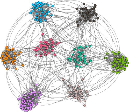
Figure 1: Graph topology. The graph is unweighted and contains $p=250$ vertices and $m=2508$ edges. Clusters have been unfolded using [22] and colored for visualization.

Figure 2: Signals on vertices $\boldsymbol{y}_{t}(i)$ and test statistic $t_{aGFSS}$. The colors correspond to the colors of the clusters, see Fig. 1. The plots represent, for each cluster, the mean of the signal with a ribbon illustrating the noise standard deviation. An abrupt change occurs at $t=400$ on the “magenta” cluster. Parameters of the aGFSS were set to $\gamma=0.3$, $\lambda=0.01$, $\Lambda=0.1$.

III Distributed and adaptive GFSS

A strategy to make Alg. 1 scalable consists of substituting the actual filter in Step 1 by a filter that can be distributed over the graph vertices as in [23, 24, 25, 26]. In contrast to these finite impulse response filters, an autoregressive moving average (ARMA) graph filter was proposed in [27, 28]. The parallel ARMA_K graph filter is defined by:

$$\boldsymbol{x}_{\ell,t}=\psi_{\ell}\boldsymbol{L}\boldsymbol{x}_{\ell,t-1}+\varphi_{\ell}\boldsymbol{y}_{t},\;\boldsymbol{x}_{\ell,-1}=\boldsymbol{0},\;\forall\ell=1\ldots K,$$ (7)

$$\boldsymbol{z}_{t}=\sum_{\ell=1}^{K}\boldsymbol{x}_{\ell,t}+c\boldsymbol{y}_{t}$$ (8)

The computation of the $i$-th entry of $\boldsymbol{L}\boldsymbol{x}_{\ell,t-1}$ by vertex $i$ only requires neighboring vertices to send it samples $\boldsymbol{x}_{\ell,t-1}(j)$. The asymptotic properties of $\boldsymbol{z}_{t}$ in Proposition 1 of Sec. IV motivates the use of an ARMA_K filter to approximate the graph filtering process used by the aGFSS. Practical problems related to the computation of parameters $c$ and $(\psi_{\ell},\varphi_{\ell})$ for $\ell=1,\ldots,K$ are discussed in Sec. V.

As noted above, the GFSS defined in (2)–(3) cannot localize the cluster where a change occurs. In order to get more insight into this statistics, it is important to recall the role played by the eigenvectors $\boldsymbol{u}_{i}$ of the (normalized) graph Laplacian matrix $\boldsymbol{L}$ in spectral clustering. Consider first the ideal case of a graph with $k>1$ connected components. The eigenvectors $\boldsymbol{u}_{i}$, $i=1,\ldots,k$ of the Laplacian are the indicator vectors of the $k$ connected components of the graph, and $\boldsymbol{u}_{i}^{\top}\boldsymbol{y}$ in (3) is proportional to the sum of the signal samples of component $i$. Replacing $h^{\ast}(\mu_{i})$ in (3) by $h^{\circ}(\mu_{i})=1$ for $1\leq i\leq k$, and $0$ otherwise, $\boldsymbol{g}(\boldsymbol{y})$ assigns to each vertex $i$ of each component $\ell$, the weighted sum of the signal samples $\boldsymbol{y}(j)$ at all vertices $j$ that belong to component $\ell$. The number of components $k$ being unknown, $h^{\ast}(\mu_{i})$ in (4) then acts as a proxy of $h^{\circ}(\mu_{i})$ that penalizes large numbers of components. If the components are connected by few edges, we can assume that this analysis is still approximately valid; see, e.g., [29, 30, 31].

This interpretation of the GFSS test statistics motivates the need to monitor, at each vertex $i$, the $i$-th entry of $\boldsymbol{g}(\boldsymbol{y})$ rather than monitoring $\|\boldsymbol{g}(\boldsymbol{y})\|_{2}$ globally. We shall denote by $\boldsymbol{g}(\boldsymbol{y})(i)$ the $i$-th entry of $\boldsymbol{g}(\boldsymbol{y})$. As an alternative to this fully local scheme, we shall consider the monitoring of each vertex $i$ including its neighborhood $N_{\mathcal{G}}(i)$. Along the same line as the standard GFSS in (2), a possible strategy consists of testing the squared 2-norm $\sum_{k\in N_{\mathcal{G}}(i)}[\boldsymbol{g}(\boldsymbol{y})(k)]^{2}$. However, given (1) which assumes that changes take the form of a constant shift $\boldsymbol{\delta}$ in the mean at all vertices of a particular cluster, we shall also focus on the coherent sum: $\sum_{k\in N_{\mathcal{G}}(i)}\boldsymbol{g}(\boldsymbol{y})(k)$. The rational behind these three test statistics is to localize the places where changes occur when they are detected. The use of an ARMA_K filter allows to implement these strategies in a fully distributed manner as shown in Alg. 2. Note that a variation of the graph topology over time can be easily taken into account by substituting $\boldsymbol{L}$ by $\boldsymbol{L}_{t}$ in Step 3: as in  [28].

1:  Learning rate $0<\lambda<\Lambda<1$, thresholds $\xi_{i}$, $i=1\ldots p$

2:  for $t=1,2,\ldots$ do

3:     for $\ell=1,\ldots,K$ do

4:        $\boldsymbol{x}_{\ell,t}=\psi_{\ell}\boldsymbol{L}\boldsymbol{x}_{\ell,t-1}+\varphi_{\ell}\boldsymbol{y}_{t}$

5:     end for

6:     $\boldsymbol{z}_{t}=\sum_{\ell=1}^{K}\boldsymbol{x}_{\ell,t}+c\boldsymbol{y}_{t}$

7:     $\boldsymbol{v}_{t}=(1-\lambda)\boldsymbol{v}_{t-1}+\lambda\boldsymbol{z}_{t}$

8:     $\boldsymbol{v}_{t}^{\prime}=(1-\Lambda)\boldsymbol{v}_{t-1}^{\prime}+\Lambda\boldsymbol{z}_{t}$

9:     $\boldsymbol{d}_{t}=\boldsymbol{v}_{t}^{\prime}-\boldsymbol{v}_{t}$

10:     $\forall i\in V$, $\boldsymbol{t}_{\text{daGFSS}}(i)=\sum_{k\in N_{\mathcal{G}}(i)}\boldsymbol{d}_{t}(k)$

11:     if $\exists i\in V$: $|\boldsymbol{t}_{\text{daGFSS}}(i)|>\xi_{i}$ then

12:        flag $t$ as a change point on the graph at vertex $i$

13:     end if

14:  end for

Algorithm 2 Distributed and Adaptive GFSS

IV Statistical analysis and test settings

The aim of this section is to derive the statistical properties of $\boldsymbol{t}_{\text{daGFSS}}(i)$ in order to set the threshold values $\xi_{i}$, $i\in V$. Using standard properties of linear dynamical systems, [32], results in [28] can be extended to the random case. Proofs are omitted due to the lack of space.

Proposition 1.

Consider the graph signal $\boldsymbol{y}_{t}=\boldsymbol{m}+\boldsymbol{e}_{t}$ with $\boldsymbol{e}_{t}$ defined as in Sec. I. If $\max_{\ell}\{|\psi_{\ell}|\}\rho(\boldsymbol{L})<1$ with $\rho(\cdot)$ the spectral radius of its matrix argument, then $\boldsymbol{z}_{t}$ is asymptotically distributed as $\boldsymbol{z}_{t}\stackrel{{\scriptstyle a}}{{\sim}}\mathcal{N}(\bar{\boldsymbol{z}}_{\infty},\boldsymbol{Q}_{\infty})$ where $\bar{\boldsymbol{z}}_{\infty}$ is the graph signal $\boldsymbol{m}$ graph-filtered by:

$$h(\mu)=c+\sum_{\ell=1}^{K}\frac{\varphi_{\ell}}{1-\psi_{\ell}\mu}$$ (9)

and:

$$\boldsymbol{Q}_{\infty}=\sum_{i=1}^{p}\kappa(\mu_{i})\boldsymbol{u}_{i}\boldsymbol{u}_{i}^{\top},\;\kappa(\mu)=\sum_{\ell,\ell^{\prime}=1}^{K}\frac{\sigma^{2}\varphi_{\ell}\varphi_{\ell^{\prime}}^{\ast}}{1-\psi_{\ell}\psi_{\ell^{\prime}}^{\ast}\mu^{2}}+\eta$$ (10)

with $\eta=c\sigma^{2}(c+2\sum_{\ell=1}^{K}\varphi_{\ell})$.

Proposition 2.

Consider the graph signal $\boldsymbol{y}_{t}=\boldsymbol{m}+\boldsymbol{e}_{t}$ with $\boldsymbol{e}_{t}$ defined as in Sec. I. If $\max_{\ell}\{|\psi_{\ell}|\}\rho(\boldsymbol{L})<1$, then $\boldsymbol{d}_{t}=\boldsymbol{v}_{t}^{\prime}-\boldsymbol{v}_{t}$ is asymptotically distributed as $\boldsymbol{d}_{t}\stackrel{{\scriptstyle a}}{{\sim}}\mathcal{N}(\boldsymbol{0},\boldsymbol{R}_{\infty})$ with:

$$\boldsymbol{R}_{\infty}=\eta\boldsymbol{Q}_{\infty},\quad\eta=\frac{\lambda}{2-\lambda}+\frac{\Lambda}{2-\Lambda}-\frac{2\lambda\Lambda}{\lambda+\Lambda-\lambda\Lambda}$$ (11)

These results are useful to set the Probability of False Alarm (PFA). If we focus on node $i$, $\boldsymbol{t}_{\text{daGFSS}}(i)\stackrel{{\scriptstyle a}}{{\sim}}\mathcal{N}(0,\sigma_{i}^{2})$ where

$$\sigma_{i}^{2}=\sum_{(k,\ell)\in N_{\mathcal{G}}(i)}\boldsymbol{R}_{\infty}(k,\ell)$$ (12)

Detecting abrupt changes over streaming graph signals by monitoring all $\boldsymbol{t}_{\text{daGFSS}}(i)$, $i\in V$, is a multiple testing problem [33]. A classical approach for controlling a global Type I error $\alpha$ within this context is the False Discovery Rate (FDR) [34], e.g., with the Benjamini-Hochberg procedure. This strategy however requires the ordering of all p-values of $\boldsymbol{t}_{\text{daGFSS}}(i)$ for all $i$, which must be performed in a centralized manner. It is also important to note that the local test statistics are not independent. A solution may consist of decorrelating $\boldsymbol{t}_{\text{daGFSS}}$, but this cannot be performed in a distributed manner. For these reasons, we propose to consider a Bonferroni correction, i.e., setting the PFA at each node to $\alpha/p$. This leads to set in Alg. 2:

$$\xi_{i}=\sqrt{2}\sigma_{i}\text{erfc}^{-1}\left(\frac{\alpha}{p}\right)$$ (13)

V Simulations

Approximating the GFSS filter (4) by the ARMA_K filter (9) is a necessary preliminary step in implementing Alg 2. Starting the summation in (3) at $i=2$ is equivalent to set $h^{\ast}(0)=0$ in (4). We observed that this strong discontinuity deteriorates the approximation of $h^{\ast}(\mu)$ by the frequency response $h(\mu)$ in (9). We propose to relax this constraint by setting $h^{\ast}(0)=1$. Note that if the standard Laplacian is used, we have $\boldsymbol{u}_{1}=\boldsymbol{1}$. Setting $h^{\ast}(0)=1$ then adds the same quantity $\sum_{k=1}^{V}\boldsymbol{y}(k)$ to each entry of $\boldsymbol{g}(\boldsymbol{y})$ and, consequently, does not affect the detection performance.

Given a filter order $K$, and similarly to the code provided in [35], the filter parameters can be computed by minimizing a quadratic loss. We considered minimizing:

$$\mathcal{J}(\boldsymbol{a},\boldsymbol{b})=\sum_{i}\left[B(x_{i})-h(x_{i})A(x_{i})\right]^{2}$$ (14)

w.r.t. $(\boldsymbol{a},\boldsymbol{b})$ where $A(x)=1+\sum_{\ell=1}^{K}\boldsymbol{a}(\ell)x^{\ell}=\prod_{\ell=1}^{K}(1-\psi_{\ell}x)$, and $B(x)=\sum_{\ell=0}^{K}\boldsymbol{b}(\ell)x^{\ell}$, over a uniform grid $x_{i}$ on the interval $(0,2)$. According to Prop. 1, this quadratic problem must be solved subject to $|\psi_{\ell}|<\rho(\boldsymbol{L})^{-1}$ for all $\ell$. Note that these constraints are related to variables $\{\psi_{\ell}\}$ while the optimization problem is solved w.r.t. $(\boldsymbol{a},\boldsymbol{b})$. To address this issue, these constraints are relaxed to the following constraints which are linear w.r.t. $\boldsymbol{a}$: $|A(x_{i})|<\beta$ for all $x_{i}$ on the grid, with $\beta$ a parameter to be set by the user. Finally, initial variables $c$ and $\{(\phi_{\ell},\psi_{\ell})\}$ were estimated from $(\boldsymbol{a},\boldsymbol{b})$ by a partial fraction expansion of $B(x)/A(x)$.

Figure 3 illustrates the approximation $h(\mu)$ of $h^{\ast}(\mu)$ with $\gamma=0.3$, for $K=4$ and $\beta=0.1$. We subsequently checked that the resulting filter $h(\mu)$ is stable. The graph used for the simulations is represented in Fig. 1. The signal $\boldsymbol{m}$ is defined as $\boldsymbol{m}(i)=k$ for all vertices $i$ in cluster $k=0\ldots 7$. The noise variance is $\sigma^{2}=7$. The total number of samples is 512 and the abrupt change at $t_{r}=400$ consisted of $\boldsymbol{\delta}(i)=0.5$ for the vertices $i$ in the pink-colored cluster, see Fig. 1. Figure 4 represents the ROC curves of the different detectors considered in this paper, and Fig. 5 provides the corresponding detection delays. Finally, Fig. 6 provides the test statistic $\boldsymbol{t}_{\text{daGFSS}}(i)$ at each node after the change point, illustrating the ability of the algorithm to localize the cluster where the change occurred. Julia code is available at github.com/andferrari/daGFSS.

VI Conclusion and perspectives

In this paper, we introduced an online change-point detection algorithm, which is fully distributed across nodes to monitor large-scale dynamic networks. We illustrated its detection and localization performance with simulated data. Perspectives of this work include change-point detection over graphs with time-varying topology.

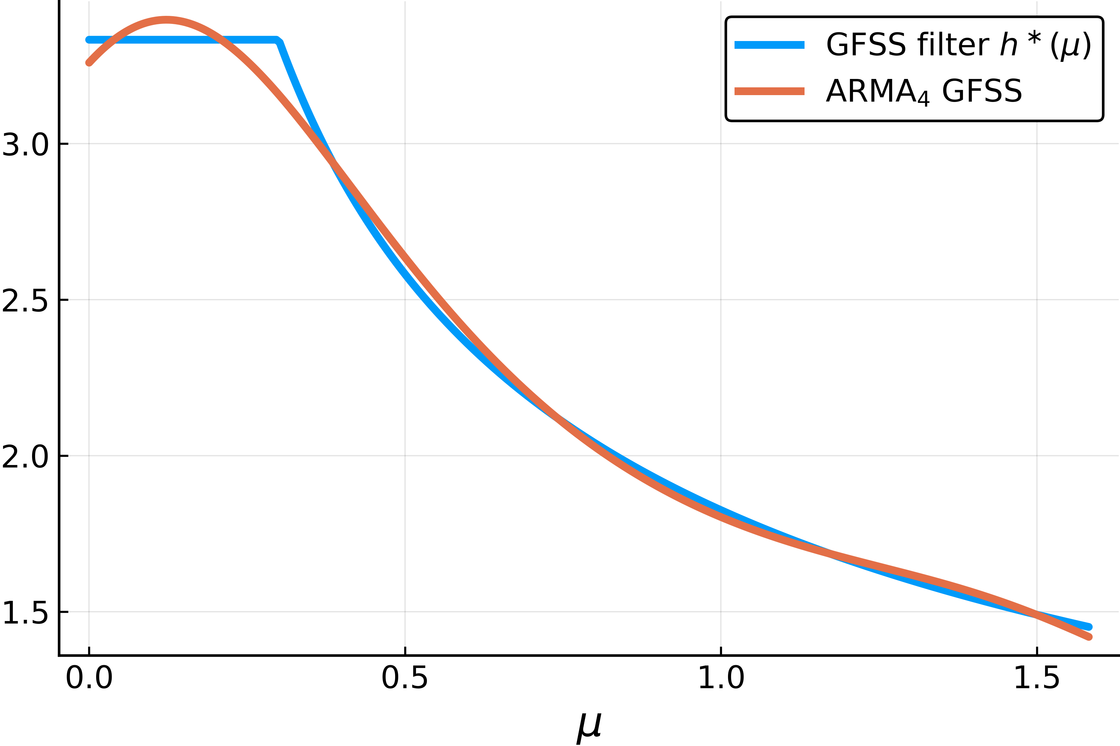
Figure 3: ARMA₄ approximation of the GFSS filter

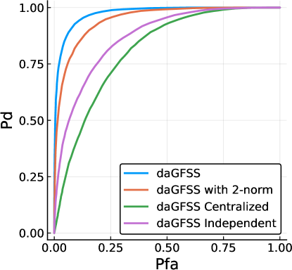
Figure 4: ROC curve. “dAGFSS”: Alg. 2, “dAGFSS with 2-norm”: Alg. 2 with test statistics based on the 2-norm, “dAGFSS centralized”: test statistic $\|\boldsymbol{d}_{t}\|_{2}$, “daGFSS independent”: test at each vertex with $|\boldsymbol{d}_{t}(i)|$.

Figure 5: Detection delay. See Fig. 4 for the labels.

 

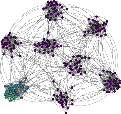
Figure 6: Test statistic $\boldsymbol{t}_{\text{daGFSS}}(i)$ for $t=t_{r}+20$.

References

- [1] J. Chen, C. Richard, and A. Sayed, “Multitask diffusion adaptation over networks,” IEEE Transactions on Signal Processing, vol. 62, no. 16, pp. 4129–4144, 2014.
- [2] J. Chen, C. Richard, and A. H. Sayed, “Diffusion lms over multitask networks,” IEEE Transactions on Signal Processing, vol. 63, no. 11, pp. 2733–2748, 2015.
- [3] R. Nassif, C. Richard, A. Ferrari, and A. H. Sayed, “Multitask diffusion adaptation over asynchronous networks,” IEEE Transactions on Signal Processing, vol. 64, no. 11, pp. 2835–2850, 2014.
- [4] ——, “Proximal multitask learning over networks with sparsity-inducing coregularization,” IEEE Transactions on Signal Processing, vol. 64, no. 23, pp. 6329–6344, 2016.
- [5] D. I. Shuman, S. K. Narang, P. Frossard, A. Ortega, and P. Vandergheynst, “The emerging field of signal processing on graphs: Extending high-dimensional data analysis to networks and other irregular domains,” IEEE Signal Processing Magazine, vol. 30, no. 3, pp. 83–98, 2013.
- [6] A. G. Marques, S. Segarra, G. Leus, and A. Ribeiro, “Stationary graph processes and spectral estimation,” IEEE Transactions on Signal Processing, vol. 65, no. 22, pp. 5911–5926, 2017.
- [7] M. A. Coutino Minguez, E. Isufi, and G. Leus, “Advances in distributed graph filtering,” IEEE Transactions on Signal Processing, vol. 67, no. 9, pp. 2320–2333, 2019.
- [8] J. Sharpnack, A. Rinaldo, and A. Singh, “Detecting anomalous activity on networks with the graph Fourier Scan Statistic,” IEEE Transactions on Signal Processing, vol. 64, no. 2, pp. 364–379, 2016.
- [9] L. Addario-Berry, N. Broutin, L. Devroye, and G. Lugosi, “On combinatorial testing problems,” The Annals of Statistics, vol. 38, no. 5, pp. 3063–3092, 2010.
- [10] E. Arias-Castro, E. J. Candès, and A. Durand, “Detection of an anomalous cluster in a network,” The Annals of Statistics, vol. 39, no. 1, pp. 278–304, 2011.
- [11] J. Sharpnack, A. Singh, and A. Rinaldo, “Changepoint detection over graphs with the spectral scan statistic,” in Proc. International Conference on Artificial Intelligence and Statistics, vol. 31, 2013, pp. 545–553.
- [12] N. Tremblay, P. Gonçalves, and P. Borgnat, “Design of graph filters and filterbanks,” in Cooperative and Graph Signal Processing. Academic Press, 2018, pp. 299–324.
- [13] A. Ortega, P. Frossard, J. Kovacevic, J. M. F. Moura, and P. Vandergheynst, “Graph signal processing: Overview, challenges, and applications,” Proceedings of the IEEE, vol. 106, no. 5, pp. 808–828, 2018.
- [14] D. M. Hawkins and Q. Deng, “A nonparametric change-point control chart,” Journal of Quality Technology, vol. 42, no. 2, pp. 165–173, 2010.
- [15] Y. Cao, L. Xie, Y. Xie, and H. Xu, “Sequential change-point detection via online convex optimization,” Entropy, vol. 20, no. 2, 2018.
- [16] Y. Xie, J. Huang, and R. Willett, “Change-point detection for high-dimensional time series with missing data,” IEEE Journal of Selected Topics in Signal Processing, vol. 7, no. 1, pp. 12–27, 2013.
- [17] D. Kifer, S. Ben-David, and J. Gehrke, “Detecting change in data streams,” in Proc. International Conference on Very Large Data Bases, 2004, pp. 180–191.
- [18] S. Liu, M. Yamada, N. Collier, and M. Sugiyama, “Change-point detection in time-series data by relative density-ratio estimation,” Neural Networks, vol. 43, pp. 72 – 83, 2013.
- [19] I. Bouchikhi, A. Ferrari, C. Richard, A. Bourrier, and M. Bernot, “Non-paramametric online change-point detection with kernel lms by relative density ratio estimation,” in Proc. IEEE Statistical Signal Processing Workshop (SSP), 2018.
- [20] ——, “Kernel based online change point detection,” in Proc. European Conference on Signal Processing (EUSIPCO), 2019.
- [21] N. Keriven, D. Garreau, and I. Poli, “Newma: a new method for scalable model-free online change-point detection,” Tech. Rep., 2018. [Online]. Available: https://arxiv.org/abs/1805.08061
- [22] V. D. Blondel, J.-L. Guillaume, R. Lambiotte, and E. Lefebvre, “Fast unfolding of communities in large networks,” Journal of Statistical Mechanics: Theory and Experiment, vol. 2008, no. 10, p. P10008, 2008.
- [23] D. I. Shuman, P. Vandergheynst, and P. Frossard, “Chebyshev polynomial approximation for distributed signal processing,” in Proc. IEEE International Conference on Distributed Computing in Sensor Systems and Workshops (DCOSS), 2011.
- [24] A. Sandryhaila, S. Kar, and J. M. F. Moura, “Finite-time distributed consensus through graph filters,” in Proc. IEEE International Conference on Acoustics, Speech and Signal Processing (ICASSP), 2014.
- [25] S. Safavi and U. A. Khan, “Revisiting finite-time distributed algorithms via successive nulling of eigenvalues,” IEEE Signal Processing Letters, vol. 22, no. 1, pp. 54–57, 2015.
- [26] S. Segarra, A. G. Marques, and A. Ribeiro, “Distributed implementation of linear network operators using graph filters,” in Proc. Annual Allerton Conference on Communication, Control, and Computing, 2015.
- [27] A. Loukas, A. Simonetto, and G. Leus, “Distributed autoregressive moving average graph filters,” IEEE Signal Processing Letters, vol. 22, no. 11, pp. 1931–1935, 2015.
- [28] E. Isufi, A. Loukas, A. Simonetto, and G. Leus, “Autoregressive moving average graph filtering,” IEEE Transactions on Signal Processing, vol. 65, no. 2, pp. 274–288, 2017.
- [29] U. von Luxburg, “A tutorial on spectral clustering,” Statistics and Computing, vol. 17, no. 4, pp. 395–416, 2007.
- [30] A. Y. Ng, M. I. Jordan, and Y. Weiss, “On spectral clustering: Analysis and an algorithm,” in Advances in Neural Information Processing Systems. University of California, Berkeley, Berkeley, United States, 2002.
- [31] J. Shi and J. Malik, “Normalized cuts and image segmentation,” IEEE Transactions on Pattern Analysis and Machine Intelligence, vol. 22, no. 8, pp. 888–905, 2000.
- [32] B. D. O. Anderson and J. B. Moore, Optimal Filtering (Dover Books on Electrical Engineering). Dover Publications, 2005.
- [33] B. Efron, Large-Scale Inference, ser. Empirical Bayes Methods for Estimation, Testing, and Prediction. Cambridge University Press, 2012.
- [34] Y. Benjamini and Y. Hochberg, “Controlling the False Discovery Rate: A Practical and Powerful Approach to Multiple Testing,” Journal of the Royal Statistical Society. Series B (Methodological), vol. 57, no. 1, pp. 289–300, 1995.
- [35] A. Loukas, “What is the most efficient graph filter? Chebyshev vs ARMA,” https://andreasloukas.blog/2017/09/04/what-is-the-most-efficient-graph-filter-tchebychev-vs-arma/.