Design- and Model-Based Approaches to Small-Area Estimation in a Low and Middle Income Country Context: Comparisons and Recommendations

Abstract

The need for rigorous and timely health and demographic summaries has provided the impetus for an explosion in geographic studies, with a common approach being the production of pixel-level maps, particularly in low and middle income countries. In this context, household surveys are a major source of data, usually with a two-stage cluster design with stratification by region and urbanicity. Accurate estimates are of crucial interest for precision public health policy interventions, but many current studies take a cavalier approach to acknowledging the sampling design, while presenting results at a fine geographic scale. In this paper we investigate the extent to which accounting for sample design can affect predictions at the aggregate level, which is usually the target of inference. We describe a simulation study in which realistic sampling frames are created for Kenya, based on population and demographic information, with a survey design that mimics a Demographic Health Survey (DHS). We compare the predictive performance of various commonly-used models. We also describe a cluster level model with a discrete spatial smoothing prior that has not been previously used, but provides reliable inference. We find that including stratification and cluster level random effects can improve predictive performance. Spatially smoothed direct (weighted) estimates were robust to priors and survey design. Continuous spatial models performed well in the presence of fine scale variation; however, these models require the most “hand holding”. Subsequently, we examine how the models perform on real data; specifically we model the prevalence of secondary education for women aged 20–29 using data from the 2014 Kenya DHS.

KEY WORDS: Survey design; spatial statistics; small area estimation, integrated nested Laplace approximations; geostatistical models.

1 Introduction

Complex, multi-stage household surveys play an important role in producing a variety of estimates of health and demographic quantities of interest, especially in low and middle income countries (LMICs). Examples of such surveys include Demographic Health Surveys (DHS) (USAID, 2019), Multiple Indicator Cluster Survey (MICS) (UNICEF - Statistics and Monitoring, 2012), AIDS Indicator Surveys (AIS) (DHS Program, 2019), and Living Standard Measurement Surveys (LSMSs) (World Bank, 2019). The lack of high quality vital registration (VR) data often necessitates the use of these household surveys in LMICs (Li et al., 2019; Wagner et al., 2018). For instance, it has been estimated that only 4% of neonatal deaths (deaths in the first 28 days of life) are recorded via high quality VR data (Lawn et al., 2014), while in 2012, 35% of births remained unregistered within a year, and 89% of these occurred in South Asia and Sub-Saharan Africa (Lawn et al., 2014). In general, VR data is more sparse and of lower quality in LMICs than in high income countries, making household surveys especially useful in these contexts.

The Sustainable Development Goals (SDGs) specify targets for a variety of health outcomes (United Nations, 2019). Household surveys are used to estimate these indices and attainment of the SDGs can then be assessed. In particular, SDG 3 calls for an end to preventable deaths of newborns and children under 5 years of age and states that all countries should aim to reduce neonatal mortality to below 12 deaths per 1,000 live births. Additionally, SDG 4 calls for improved education for all, and for all people to complete their secondary education with, in particular, the elimination of inequalities in education due to gender or location. As important as it is to estimate relevant indicators at the country level, the SDGs specifically call for estimates at finer spatial scales. Hence, developing statistical models that can accurately account for the sampling design, while producing estimates at subnational scales, is of great importance.

Estimates of demographic indicators can also be used to highlight areas in need of intervention and to examine associations between relevant covariates and health outcomes. The Equitable Impact Sensitive Tool (EQUIST) (UNICEF, 2019), for instance, is designed to inform decision-makers using a variety of data and model output visualizations. Policymakers can use such tools, as well as other forms of model output and analysis to, for example, create vaccination initiatives targeting areas with a high disease burden, identify possible factors influencing disease prevalence and mortality risk, and erect community-based care programs in order to improve quality of care while increasing coverage to those that need it most while reducing cost. Some of these applications, including community-based care programs, are discussed in detail in Chapters 14 and 15 of Black et al. (2016).

In spite of the ubiquity of multi-stage household surveys and their importance in estimating health indices and planning interventions, classical techniques for analyzing survey data that can account for the survey design often have difficulty producing estimates at the required spatial resolutions (interventions are often made at the Admin2 level). For example, weighted (direct) estimates, often have large associated variances at the Admin2 level, due to data sparsity. To improve estimation in such situations, a number of small area estimation (SAE) methods have been proposed (Rao and Molina, 2015) including those that extend upon the seminal Fay-Herriot model (Fay and Herriot, 1979). These methods not only acknowledge the survey design, but also “borrow strength” from data in nearby areas to produce reliable estimates with smaller uncertainty intervals (Marhuenda et al., 2013; Chen et al., 2014; Mercer et al., 2015; Congdon and Lloyd, 2010; You and Zhou, 2011; Porter et al., 2014; Vandendijck et al., 2016; Watjou et al., 2017). These approaches are all based on discrete spatial models, which are based on arbitrary neighborhood structures, which may be more or less realistic, depending on the context and geography.

A number of papers have used continuous spatial models to analyze health and demographic outcomes using survey data (Wardrop et al., 2018; Gething et al., 2016; Golding et al., 2017; Utazi et al., 2018; Gething et al., 2015; Osgood-Zimmerman et al., 2018; Graetz et al., 2018; Diggle and Giorgi, 2016; Giorgi et al., 2018; Diggle and Giorgi, 2019). Included in this list are publications from WorldPop and the Institute for Health Metrics and Evaluation (IHME), both of which are large-scale producers of health and demographic maps. In these references, all of the models ignore the stratification; in addition WorldPop routinely ignore the clustering also. In general, ignoring the design results in biased estimates and inaccurate uncertainty intervals. No study has been conducted to explore the effects of ignoring design stratification and cluster level overdispersion in the LMIC context, and here we aim to fill this gap in the literature, by comparing a variety of spatial modeling approaches, under different levels of stratification and clustering.

In this paper we explore the performance of different design- and model-based methods, when applied to simulated data. We will also apply these methods to analyze two outcomes recorded in the 2014 Kenya DHS, the proportion of women between the ages of 20 and 29 who have secondary education, and the neonatal mortality rate (NMR). Section 2 describes the data we will use in this analysis and Section 3 introduces the models that we compare and apply. Section 4 describes the simulation study and in Section 5 we apply the models to the secondary education outcome, reporting predictions, uncertainties, and using cross validation to assess the out of sample performance of each of the models. We discuss the results as well as our conclusions in Section 6. Appendices A and B give details on the modeling and the simulation study respectively, and Appendix C gives additional results related to the secondary education example.Lastly, Appendix D describes an application of the models to NMRs in Kenya from 2010–2014.

2 Data

The DHS Program uses a set of consistent sampling approaches from country to country, with methods described in the 2012 DHS Sampling and Household Listing Manual (ICF International, 2012, Sec. 5.2, p. 80–85). This standard design is a stratified two-stage cluster sampling scheme with stratification by county crossed with urban/rural. The first sampling stage involves selecting enumeration areas (EAs) using probability proportional to size (PPS) sampling, where the probability of sampling each EA is proportional to the listed number of households in that EA, and the second stage involves simple random sampling of (typically) 25 households within each EA. Mothers within the household are then asked a number of questions about their children, and, if any died, the mothers are asked about those children’s deaths. The 2014 Kenya DHS (KDHS, 2014) follows the typical DHS scheme, though is powered to the county level so that 1,612 clusters are sampled out of the 96,251 total EAs that were in the 2009 Kenya Population and Housing Census (Kenya National Bureau Of Statistics, 2014). Of these clusters, 995 are urban while 617 are rural, with urban areas oversampled in the majority of the 47 counties. Mombasa and Nairobi are entirely urban and the remaining 45 counties have both urban and rural areas, so that there are 92 strata in total.

In order to be able to generate spatial maps of urbanicity, we use 1km $\times$ 1km gridded population density surfaces from WorldPop (Stevens et al., 2015; Tatem, 2017) as plotted in the left panel of Figure 1. The 2010 and 2015 population density maps are interpolated assuming a constant rate of population growth to produce the 2014 population density map used throughout this paper. The 2009 Kenya Population and Housing Census provides information on the proportion of the population within each county that is urban and rural, and we generate urbanicity maps by thresholding the population density maps within each county at the level required to achieve this proportion. This results in the urbanicity map given in the right panel of Figure 1.

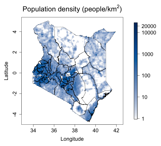
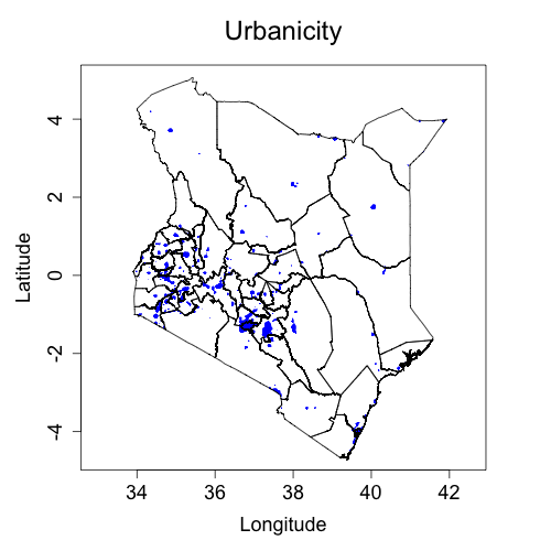
Figure 1: Left: WorldPop based population density estimates. Right: urban areas in Kenya used in this analysis are depicted in blue. Areas are determined to be urban versus rural based on thresholding population density.

3 Methods

3.1 Models

We first describe notation in the scenario in which we wish to estimate NMRs, so that the denominators are the number of children that were born in the relevant period, and the response is whether a death occurred in the first month after birth. Let $Y_{ck}=0/1$ represent the binary response for child $k$ in cluster $c$ with the total number of deaths in each cluster being $Y_{c}=\sum_{k\in\mathcal{B}_{c}}Y_{ck}$ where $\mathcal{B}_{c}$ is the set of indices of the children in cluster $c$ that are sampled. We let $\mbox{\boldmath$x$}_{c}$ be the spatial location of cluster $c$. Associated with location $\mbox{\boldmath$x$}_{c}$ is a county, which will be denoted $i[c]$, and the set of spatial locations that are urban is denoted $U$. We now describe the different models considered; in general, we focus on inference at the county level, since this is often the target of inference.

Naive: Ignoring the sampling design, we fit a binomial model to the county-level data, without accounting for the sampling design. In this case, we assume the probability of mortality for child $k$ in cluster $c$ is the same for all children in county $i$,

$$\log\left(\frac{p_{ck}}{1-p_{ck}}\right)=\beta_{i[c]},$$

where the models are fit independently to the data from each county. The targets of inference are the county-level probabilities $\text{expit}(\beta_{i})$, $i=1,\dots,47$.

Direct: County-level direct estimates, $\widehat{p}^{~{}\mbox{\tiny{DIR}}}_{i}$, are calculated using a weighted estimator that account for the survey design. The weights are proportional to the inverse of the probability of sampling each child. This estimator is reliable for large samples, but for small samples, will have high variance (Rao and Molina, 2015). Weighted estimators can yield estimates that lie on the boundary and variance instability in small samples. These problems mean that yearly estimates at the Admin2 level are typically not reliable when based on a DHS with around 400 clusters (a typical design).

Smoothed Direct: Following the approach of Mercer et al. (2015) we calculate $Z_{i}~{}=~{}\mbox{logit}(\widehat{p}^{~{}\mbox{\tiny{DIR}}}_{i})$ along with its associated (design-based) variance estimate $\widehat{V}_{i}$. We assume $Z_{i}|\eta_{i}~{}\sim_{ind}~{}\mbox{$N$}(\eta_{i},\widehat{V}_{i})$ with linear predictor,

$$\eta_{i} =\beta_{0}+\frac{1}{\sqrt{\tau}}(\sqrt{\phi}S_{i}+\sqrt{1-\phi}\delta_{i}),$$

where $S_{1},\dots,S_{47}$ and $\delta_{1},\dots,\delta_{47}$ are respectively mean zero county level intrinsic conditional autoregressive (ICAR) terms and independent and identically distributed (iid) Gaussian random effects. The ICAR model, described in Besag et al. (1991), is a discrete spatial model and assumes the effect in each area arises from a normal whose mean is the average of the effects in neighboring areas. We apply a sum-to-zero constraint $\sum_{i=1}^{47}S_{i}=0$ to the ICAR terms to make the intercept identifiable. The parameterization adopted is a variation of the model introduced in Simpson et al. (2017) and named the BYM2 model in Riebler et al. (2016), since it is a reparameterization of the model originally introduced by Besag et al. (1991). The total precision of the county level components of the model is $\tau$ and $\phi$ represents the proportion of the total variance that is spatial. Under this approach the posterior distribution is obtained for the county level probabilities: $p^{~{}\mbox{\tiny{SM-DIR}}}_{i}=\mbox{expit}(\eta_{i}),$, $i=1,\dots,47.$ This model produces a design consistent estimate of the NMR, since if the entire population is sampled, the direct estimate has an associated variance estimate $\widehat{V}_{i}=0$ for $i=1,\dots,47$, and so is immovable with respect to the prior. The space-time version of this model has been used in an extensive study of under 5 mortality in 35 countries in Africa over the period 1980–2015 (Li et al., 2019). This model can alleviate some of the high variance problems of the direct estimates, but still struggles with boundary estimates and undefined variances.

Model-based approaches: For the model-based spatial approaches, we assume that $Y_{c}|p(\bm{x}_{c})\sim\mbox{Bin}(n_{c},p(\bm{x})),$ where $n_{c}$ is the total number of children sampled in cluster $c$. The underlying risk at location $\bm{x}_{c}$ for cluster $c$ is modeled as

$$\log\left(\frac{p(\bm{x}_{c})}{1-p(\bm{x}_{c})}\right)=\beta_{0}+u(\bm{x}_{c})+\beta^{\mbox{\tiny{URB}}}I(\bm{x}_{c}\in U)+\epsilon_{c},$$ (1)

where $\beta_{0}$ is the intercept, $u(\bm{x}_{c})$ is a spatial random effect, $\beta^{\mbox{\tiny{URB}}}$ is the association with the cluster being urban (as compared to rural), and $\epsilon_{c}$ is an iid Gaussian cluster random effect with variance $\sigma_{\epsilon}^{2}$. This term is sometimes described as the “nugget” and is often taken to reflect the combination of unmodeled sampling variability and small-scale variation.

The first model-based approach is termed BYM2 and uses the spatial random effect $u(\bm{x})=\frac{1}{\sqrt{\tau}}(\sqrt{\phi}S_{i[\bm{x}]}+\sqrt{1-\phi}\delta_{i[\bm{x}]}),$ where we use $i[\bm{x}]$ to denote the county which which $\bm{x}$ belongs, and the structure of the model follows the description for the smoothed direct model. This binomial model naturally deals with 0 or $n_{c}$ outcomes.

The second model-based approach is termed SPDE and uses a Gaussian process (GP) for the spatial random effect, $u(\cdot)\sim\mbox{GP}(0,\mbox{\boldmath$\theta$})$ with $\mbox{\boldmath$\theta$}=[\sigma_{s}^{2},\rho]$. The marginal variance is $\sigma_{s}^{2}$ and the spatial range at which the correlation is approximately 0.1 is $\rho$. Note that the GP we use is the solution to a stochastic partial differential equation (SPDE) which is approximated by a particular Gaussian Markov Random Field (GMRF) defined on a fine triangular mesh (Lindgren et al., 2011).

For both BYM and SPDE, we consider four variations of (1): including or not including the association with urban, and including or not including the cluster (nugget) effect. Models without and with urban effects are labeled as ‘u’ and ‘U’, respectively. Similarly, models without and with cluster effects are labeled as ‘c’ and ‘C’, respectively. Table 1 summarizes the eight alternatives for BYM2 and SPDE.

Models	Linear predictor extra effects
BYM2uc/SPDEuc	–
BYM2uC/SPDEuC	$\epsilon_{c}$
BYM2Uc/SPDEUc	$\beta^{\mbox{\tiny{URB}}}I(\mbox{\boldmath$x$}_{c}\in U)$
BYM2UC/SPDEUC	$\beta^{\mbox{\tiny{URB}}}I(\mbox{\boldmath$x$}_{c}\in U)+\epsilon_{c}$

Table 1: Variations of model-based approaches used in the analysis. The subscript symbols ‘U’ and ‘u’ indicate whether or not an urban effect is present in the linear predictor, while ‘C’ and ‘c’ indicate whether or not an iid cluster effect is included. All models include intercept and the spatial effect.

For the continuous (SPDE) model, if we knew the complete list of EA locations in the sampling frame, we could perform predictions for the county level by using the posterior distribution of a weighted sum over the EA locations. In the absence of such a list, we can describe the probability surface at unobserved locations by $p(\bm{x})$ via (1), and aggregate by continuously integrating the spatial probability surface with respect to population density. Let $p_{i}$ denote the county level estimates for county $i$, then

$$p_{i}=\int_{A_{i}}p(\mbox{\boldmath$x$})\times q(\mbox{\boldmath$x$})~{}d\mbox{\boldmath$x$}\approx\sum_{j=1}^{m_{i}}p(\mbox{\boldmath$x$}_{j})\times q(\mbox{\boldmath$x$}_{j}),$$ (2)

where $A_{i}$ is the geographical extent of area $i$, $q(\mbox{\boldmath$x$})$ is the population density at location $x$, and $m_{i}$ is the number of grid cells with centroids in area $i$ that is used to approximate the continuous integral.

For the BYM2 model, a continuous population density surface is not needed since the probabilities are modeled as constant within each area, and we can use

$$p_{i} = \mbox{expit}\left(\beta_{0}+\frac{1}{\sqrt{\tau}}(\sqrt{\phi}S_{i}+\sqrt{1-\phi}\delta_{i}\right)q_{i}$$

$$+ \mbox{expit}\left(\beta_{0}+\beta^{\mbox{\tiny{URB}}}+\frac{1}{\sqrt{\tau}}(\sqrt{\phi}S_{i}+\sqrt{1-\phi}\delta_{i}\right)(1-q_{i}),$$

where $q_{i}$ is the proportion of the target population in county $i$ that is rural. Further details of accounting for the cluster effects and performing the spatial aggregation may be found in Appendix A.

Both Worldpop and IHME use a continuous GP model in the context of the analysis of DHS (and other) household survey data, without adjustment for the stratification. IHME include a cluster effect in their model, and for aggregation add a nugget contribution at the pixel-level, while Worldpop do not include a nugget.

3.2 Inference

Penalized complexity (PC) priors were introduced in Simpson et al. (2017), and penalize a model’s “distance”, on an appropriate scale, from a simple “base” model. For example, for iid random effects arising from a zero mean Gaussian distribution with variance $\sigma^{2}$, the base model corresponds to $\sigma=0$. Following Fuglstad et al. (2019), we set a joint PC prior on the continuous spatial standard deviation and effective range parameters $\sigma_{s}$ and $\rho$, respectively. We use the joint PC prior described by Riebler et al. (2016) on the BYM2 standard deviation $1/\sqrt{\tau}$ and the proportion of variation that is spatial, $\phi$. We also set a marginal PC prior on the cluster effect standard deviation parameter $\sigma_{\epsilon}$. The priors in the simulation study and in the application are set so that the median of the prior for $\rho$ is at roughly one fifth the diameter of the spatial domain, and so that $P(\sigma_{s}>1)=P(1/\sqrt{\tau}>1)=P(\sigma_{\epsilon}>1)=0.01$. This implies that the continuous spatial effects, BYM2 effects, and cluster effects for the spatial smoothing models each have a 95% prior chance of lying between 0.5 and 2 on an odds scale. The PC prior for the spatial proportion in the BYM2 model, $\phi$, is given a $2/3$ prior probability of being less than $1/2$, implying that we slightly favor the iid county level effects when apportioning residual variation. We choose this prior on $\phi$ in order to promote less complex models with a smaller spatial contribution.

All design-based estimates were obtained using the svyglm function within the survey package (Lumley, 2004, 2018) in the R programming language. Each of the spatial models can be fitted using the integrated nested Laplace approximation (INLA) approach introduced in Rue et al. (2009), a method for fitting Bayesian models without the computational difficulties of Markov Chain Monte Carlo (MCMC) and implemented in the INLA package in R. The direct, smoothed direct and binomial BYM2 models are available in the SUMMER package (Martin et al., 2018). Code to reproduce the results can be found at https://github.com/paigejo/NMRmanuscript, and the 2014 Kenya DHS data can be requested from https://dhsprogram.com/.

4 Simulation Study

4.1 Comparison Measures

In this section, we describe an extensive simulation study in which we compare various models, in particular with respect to the inclusion of strata and cluster effects. We do this for multiple simulated populations and survey designs in order to test the models under a variety of circumstances. As in Section 3, the nominal response is a binary indicator of whether or not death occurred within the first month of life.

We evaluate the model predictions at the county level using bias, mean squared error (MSE), the continuous rank probability score (CRPS), coverage of 80% intervals, and width of 80% intervals. All scoring rules are calculated on the probability scale. Note that CRPS is a strictly proper scoring rule (Gneiting and Raftery, 2007) that accounts for both predictive accuracy as well as accuracy of the uncertainty of the predictive distribution. Given the cumulative distribution function of the predictive distribution of a proportion in the finite population, $F$, and an empirical proportion response $y/n$, the CRPS is defined as:

$$\mbox{CRPS}(F,y) =\sum_{\tilde{y}=0}^{n}(F(\tilde{y}/n)-1\{\tilde{y}\geq y\})^{2}.$$

Small values of CRPS are desirable.

The reported scoring rules are calculated using predictive distributions that have been calculated at the county level. The reported scores are the averages over counties and repeated surveys, and the full set of calculated scoring rules are given in Appendix B.3.

4.2 Simulation Setup

In order to generate a true, underlying population from which we can draw surveys, we first spatially partition Kenya into urban and rural zones by thresholding population density so that the proportion of population in each county that is urban matches the 2009 Kenya Population and Housing Census. We then simulate all 96,251 census EA locations such that the number in each of the 92 strata matches the true number, as given in the 2009 census. The EA locations in our simulated population are drawn proportional to population density within each strata. This information is all available in the Kenya DHS final report (KDHS, 2014).

The number of households in each EA, as well as the number of mothers per household and children born per mother per year, are simulated based on the corresponding empirical distributions in the true population stratified by urban/rural. In order to estimate the empirical distribution for the number of households per EA, we take the maximum household ID sampled per cluster in the 2014 Kenya DHS as an estimate for the number of households in each EA. For empirical distributions of the number of children born per mother per year we only include children living in the same house as their mother, since children living in a different house than their mother only account for about 5% of all children according to available census data.

We compared the models in eight distinct scenarios. We simulate four different complete populations from the models (with associated names): constant risk (Pop_suc), spatially-varying risk (Pop_Suc), spatially-varying risk with an urban association (Pop_SUc), and spatially-varying risk with an urban association and a cluster effect (Pop_SUC). Note that in the subscript labels for the populations, we again use U/u and C/c to respectively indicate the presence of urban and cluster effects, and we additionally use S/s to indicate presence of a continuous spatial effect. In the case where we include spatial, urban, and cluster effects, we simulate NMRs at all 96,251 spatial locations using the SPDE model described above with an effective correlation range of 150km, and with parameters $\beta_{0}=-1.75$, $\sigma_{s}^{2}=0.15^{2}$, $\sigma^{2}_{\epsilon}=0.1^{2}$, and $\beta^{\mbox{\tiny{URB}}}=-1$. For “typical” rural/urban areas, with random effects of zero, the prevalences are 17%/6%. Within each of these four scenarios we carry out “Unstratified” and “Stratified” sampling, always taking 1,612 clusters to match the 2014 Kenya DHS. In the Unstratified design, we fix the total number of clusters in each county to be the same as in the Kenya DHS, and choose the proportion of urban and rural cluster within each county to match the proportion of the urban and rural population in that county. In the Stratified design, we sample urban and rural clusters at different rates for each county so as to match the proportion of urban clusters in each county of the 2014 Kenya DHS, obstaining 995 and 617 urban and rural clusters respectively. Conditional on the total number of urban and rural clusters for each of the 92 strata, we use PPS sampling to determine which clusters are included in the surveys, sampling clusters with probability proportional to the number of households in each strata. Within each EA, 25 households are chosen at random to be included in the cluster sample. The simulated population and a single simulated survey based on the Stratified design are shown in Figure 2.

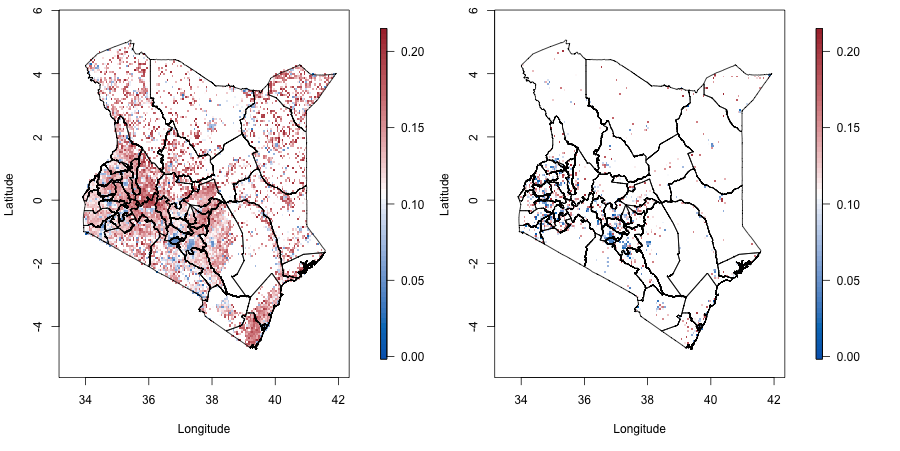
Figure 2: Simulated population of Kenya and associated NMRs (left), and an example simulated dataset based on the “Stratified” design (right).

4.3 Simulation Results

The scoring rules summarizing the main results for the stratified design are plotted in Figure 3, and parameter summary statistics are given in Appendix B.3. Scoring rules for additional model variations and designs are compared in Appendix B.2. When interpreting these scoring rules, it is important to keep in mind that SDG 3 calls for a reduction in NMRs to 12 deaths per 1,000 children, which corresponds to 120 $\times 10^{-4}$ children. When absolute bias is large relative to this number, it is an indicator of poor model performance. Since we are especially interested in the performance of the models in a not atypical scenario in which spatial, urban and cluster effects must be accounted for, we will be discussing Pop_SUC under a Stratified design unless we state otherwise.

Of the direct, smoothed direct, BYM2_UC, and SPDE_UC models, the BYM2_UC model performed the best in terms of CRPS, MSE, coverage, and CI width. Although the BYM2_UC model was slightly positively biased, the precision of its central predictions and the well-calibrated predictive distribution and uncertainty intervals led to accurate coverages and good predictive performance.

Interestingly, although the SPDE_UC model matched the model used to simulate the data, it did not perform well in terms of MSE. Its MSE was $1.24\times 10^{-4}$ compared to $0.41\times 10^{-4}$ for the BYM2_UC model, $0.63\times 10^{-4}$ for the smoothed direct, and $0.72\times 10^{-4}$ for the direct model. Although SPDE_UC model estimates were somewhat positively biased, the high level of MSE was mainly due to high variances (see results in Appendix B.3.2). In spite of this, the SPDE_UC model had a CRPS of $4.7\times 10^{-3}$, which was comparable to the value of $4.6\times 10^{-3}$ for the smoothed direct model, and was better than the direct model value of $4.9\times 10^{-3}$. Additionally, the coverage of the SPDE_UC model was 82%, second in accuracy only to the BYM2_UC model. Hence, although the central predictions of the SPDE model were somewhat variable, the uncertainty of the predictive distribution was well-calibrated.

The smoothed direct and BYM2_Uc models had the smallest magnitude of bias. An advantage of the smoothed direct model is that, regardless of the population and survey scheme considered, the model performed well from the standpoints of MSE, CRPS, bias, and coverage. Although the coverage for the Pop_suc (constant risk) population was over 90%, so were the coverages of the BYM2 models. Additionally, the constant risk setting is not realistic, and therefore should not be focused on too much. Overall, the smoothed direct model was robust in terms of its predictive accuracy and uncertainty.

The tables in Appendix B.3 show that the spatial smoothing models were better at estimating the urban effect than the intercept, although inclusion of an urban effect improved intercept estimation. For instance, for the SUC population under the Stratified design, the BYM2_UC model average intercept estimate was -1.67, whereas the average BYM2_uC estimate was -1.99. The equivalent values for the SPDE_UC and SPDE_uC models were respectively -1.69 and -1.86. Although the models including urban effects were generally closer to the truth than models without urban effects, there still was some bias in the parameter estimates. The urban effect tended to be better estimated, however. The average estimate for the BYM2 and SPDE ‘UC’ models were both -1.0.

Models that did not account for urbanicity either indirectly via sampling weights or directly as a covariate had relatively poor performance from MSE, bias, CRPS, and coverage standpoints. Even for populations without urban associations or under the unstratified design, there was little downside to including urban effects so long as the proportion of children in urban and rural areas was not poorly estimated (so that the area averaging was poorly performed). Including urban effects led to MSE, bias, CRPS, credible interval width, and coverage that was on average either better or nearly equal to the corresponding models without urban effects throughout all simulated populations and designs. The benefit of including urbanicity as a covariate was increased under the Stratified design relative to the Unstratified design since urban and rural areas were not sampled proportionately in that case.

In general, the inclusion of a cluster effect led to better or equally good predictions, compared to when cluster effects were not included, in terms of MSE and CRPS, as shown in Appendix B.2. This is especially true for the SPDE model, whose predictions were more influenced by the inclusion of cluster effects. Although the MSE and bias of the BYM2_uc and BYM2_uC models were essentially the same, the inclusion of the cluster effect led to a dramatic improvement in coverage from 55% to 68%, indicating that cluster effects can lead to more accurate measures of uncertainty. Although the BYM2_Uc model arguably performs slightly better than the BYM2_UC model in terms of its MSE and CRPS, the coverage of the BYM2_UC model is better, and the uncertainty intervals are more conservative. To summarize, these simulations suggest that, amongst the BYM2 models, the BYM2_UC model is a robust choice for the analysis of DHS household survey data.

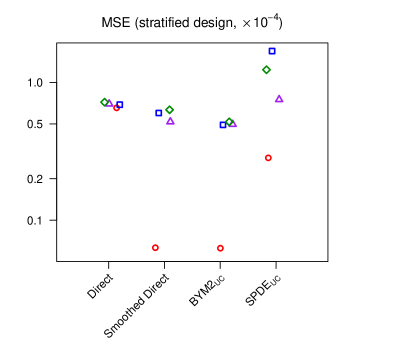
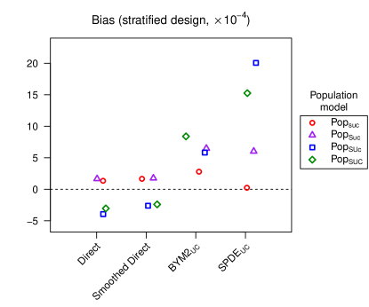
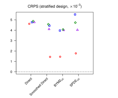
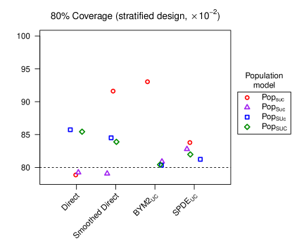
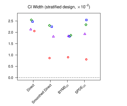
Figure 3: County level scoring rules plotted for each of the simulated populations and the main models considered for the Stratified design. The labels s/S, u/U, and c/C denote whether or not spatial, urban, and cluster effects are included in the models respectively. The “Population model” denotes the method by which the data were generated.

5 Prevalence of Secondary Education for Women in Kenya

Although some prior results suggest that under-5 mortality rates and other health outcomes are influenced by urbanicity in Sub-Saharan Africa (Wakefield et al., 2019; Ntenda et al., 2014; Antai and Moradi, 2010; Balk et al., 2004; Root, 1997; Defo, 1994; Pezzulo et al., 2016), we did not find strong evidence of a marginal association between NMRs and urbanicity in Kenya. An analysis of NMRs from the 2014 Kenya DHS is presented in Appendix D. In this section, we focus on secondary education completion rates for women aged 20–29 in 2014 using the Kenya DHS. This outcome displays a strong association with urbanicity. We focus on the age range because most women that will complete their secondary education have already done so by that age, and also because we found evidence of generational differences in secondary education levels among women. Weighted estimates of the secondary education levels at the county level are plotted in the top left panel of Figure 4, and we see large variability in the estimates, though there is a large amount of uncertainty in many of these estimates (bottom left panel).

5.1 Prevalence Mapping

Here we provide only a small number of summaries, Appendix C gives more detailed results. Central predictions as well as interval widths for the direct, naive, smoothed direct, and the full (‘UC’) spatial smoothing models are shown in Figure 4. The top row (point) estimates are quite similar, since there are a large number of clusters, but close examination shows there are differences. Prevalence tended to be higher in the central, southern, and western counties, and tended to be lower and with greater uncertainty in the more rural counties to the north and east. Appendix C gives full numerical results and here we summarize. The odds (with associated 80% CIs) of young women in urban clusters completing their secondary education are larger, relative to rural clusters, by 210% (185%, 236%) or 170% (148%, 193%) as respectively estimated by the BYM2_UC and SPDE_UC models.

Results in Appendix C shows that the smoothed direct, SPDE_UC, and BYM2_UC models all estimate that the secondary education levels for young women in Kenya was highest in Nairobi, with point estimates (80% CIs) of 0.54 (0.49, 0.58), 0.55 (0.51, 0.58), and 0.53 (0.50, 0.57) respectively. On the other hand, Mandera was estimated to have the lowest secondary education levels for all models except for the SPDE_UC model (for which Turkana was estimated to have the lowest secondary education levels) with point estimates (80% CIs) of 0.088 (0.061, 0.13), 0.081 (0.058, 0.11), and 0.085 (0.060, 0.12) respectively. While Nairobi is designated as completely urban, approximately 18% of the population of Mandera is urban, which is very close to the median for counties in Kenya. This suggests there are other factors in Mandera that are reducing the secondary education prevalence for the women living there.

The credible interval widths were largest for the direct model and smallest for the SPDE_UC model. Of the displayed spatial smoothing models, the smoothed direct model had the largest predictive variances. Both the smoothed direct and the BYM2 models had relatively high uncertainties for counties with fewer neighbors, whereas the SPDE model variances tended to be high near the edges and where the number of clusters were spatially distant from each other. In central and west Kenya, where the sampled clusters tended to be denser, the SPDE model had lower predictive variances relative to the discrete spatial models.

Figure 5 shows the continuous, 5km$\times$5km pixel level predictions and credible interval widths for the SPDE_uC and SPDE_UC models. The urban effect is especially visible in the predictions of the SPDE_uC, since it oversmooths the effect of the urban areas into nearby rural regions. Interestingly, secondary education prevalences appear to be high not only in urban areas, but also in rural areas bordering urban centers. This indicates that some of the urban/rural association (which was smaller for the SPDE model) is being absorbed into the spatial field. In general, we are nervous about presenting pixel-level maps, and far more comfortable with area-level summaries. Figure 5 clearly shows that care that must be taken with stratification. In order to maintain confidentiality, the geographical locations of the DHS clusters are displaced (jittered): urban clusters by up to 2km, rural clusters by up to 5km, with a further 1% by up to 10km, which is another reason that pixel-level maps should not be over-interpreted.

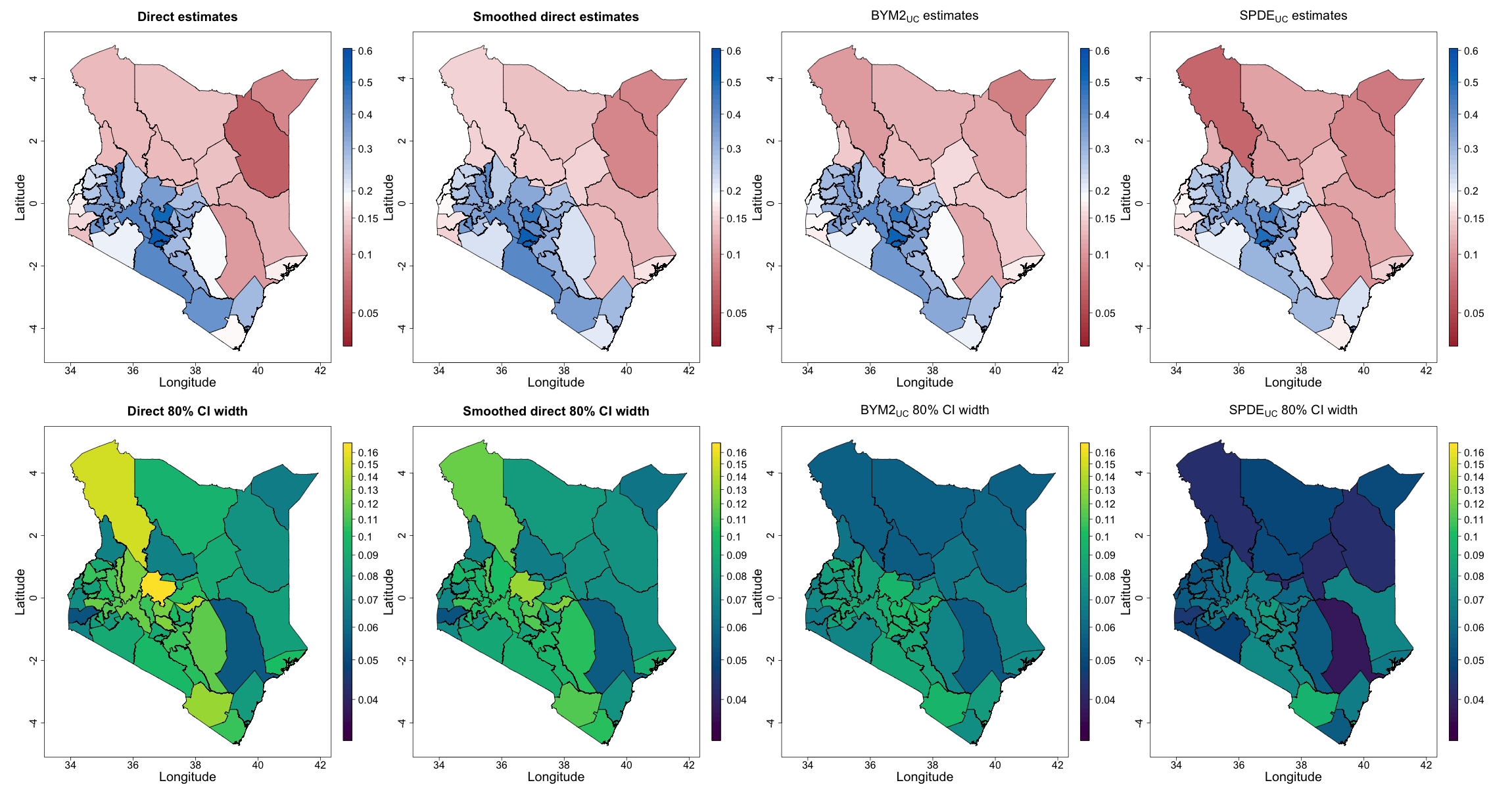
Figure 4: Kenya county level 2014 secondary education predictive estimates (top) and 80% uncertainty interval width (bottom) for women aged 20–29. The BYM2 and SPDE model predictions include both urban and cluster effects.

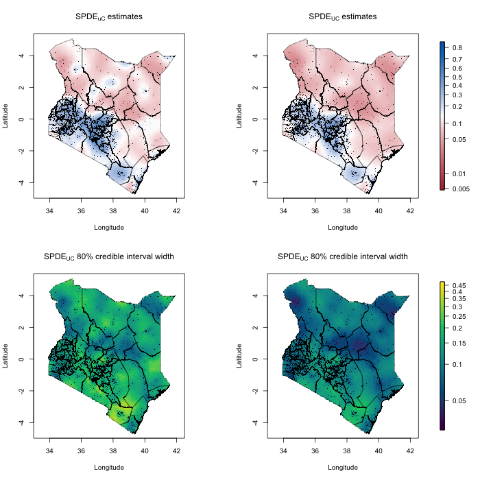
Figure 5: Kenya 5km $\times$ 5km pixel level 2014 secondary education predictive mean (top) and 80% uncertainty interval width (bottom) for women aged 20–29. Results are shown for the SPDE_uC (left) and SPDE_UC (right) models.

5.2 Validation

We calculate a number of scoring rules at the cluster level to evaluate the spatial smoothing models. We compute the scoring rules by leaving out data from one county at a time and averaging the scoring rules over all 47 such experiments. We carry out the validation out at the county level, since this is generally the target of inference. In addition to calculating MSE (broken down into variance and bias and in urban as well as rural areas) we also compute CRPS, the deviance information criterion (DIC), and the conditional predictive ordinate (CPO). The naive, direct, and smoothed direct models are fit at the county level, so we did not include their validation results, since they are not comparable with the cluster level data models.

The SPDE_Uc and SPDE_UC models had the two best average MSEs, and the SPDE_Uc model has the best CPO and CRPS. The SPDE_UC had better MSE than the Uc model, but it had worse CPO and CRPS. In terms of MSE and CRPS, the BYM2_Uc model also performed well, and had the smallest magnitude of bias. The good performance of the SPDE models may be due to their ability to model continuous changes in secondary education near the borders of each county, whereas the BYM2 models are unable to distinguish between clusters at the border of a county versus clusters in the center. In Appendix C we see that the spatial standard deviation (SD) of the SPDE_UC model is estimated to be 0.91, whereas the cluster effect is estimated to have a SD of 0.65. This is a higher proportion of variability going into the spatial term than in the BYM2_UC model, which has a total variance of county level random effects estimated to be 0.57 and a cluster variance estimated to be 0.71. This suggests the ability of the SPDE model to predict continuously through space gives it an advantage when making predictions at the cluster level.

	BYM2				SPDE
	uc	uC	Uc	UC	uc	uC	Uc	UC
MSE ($\times 10^{-2}$)
Average	5.9	6.0	5.1	5.2	5.6	5.4	5.0	4.9
Urban	7.2	7.2	6.2	6.2	7.1	6.8	6.2	6.0
Rural	5.0	5.2	4.5	4.5	4.6	4.5	4.2	4.2
Var ($\times 10^{-3}$)
Average	59	59	51	52	56	53.8	50	49
Urban	61	62	62	62	63	60	62	60
Rural	45	45	45	45	45	42	42	42
Bias ($\times 10^{-3}$)
Average	6.0	10.5	1.0	5.6	-15.0	-6.2	-3.6	-3.2
Urban	-105	-103	11.1	8.3	-93	-91	1.0	3.1
Rural	77	83	-5.4	4.0	35	48	-6.5	-7.2
CPO
Average	0.22	0.21	0.25	0.24	0.26	0.25	0.27	0.26
CRPS
Average	0.17	0.21	0.16	0.18	0.17	0.18	0.15	0.17

Table 2: Validation results calculated at the cluster level when leaving out one county at a time for the 2014 Kenya DHS secondary education data for women aged 20–29. The worst entries in each row are in italics, while the best entries in each row are in bold. In the table, the figures are rounded, but minimum and maximum were evaluated with more significant figures.

6 Discussion and Conclusions

Direct estimators remain the gold standard, provided there are sufficient data for an associated variance that is of acceptable size. The smoothed direct estimator can reduce the variance using the totality of data, albeit with an introduction of small bias, due to the smoothing. When the direct estimates are unreliable, one is lead to modeling at the cluster-level, and one must use a model that is consistent with the design. In this paper, we introduced a binomial sampling model with discrete spatial random effects, and it performed well in the simulations and in the real application. We have also been experimenting with a beta-binomial that allows for overdispersion (within-cluster variation). Such approaches with discrete spatial models do not deal well with combining data at different geographical resolutions, and this is where the continuous spatial model is appealing. Unfortunately, aggregation with this model is the most difficult, since a population surface is required, and this needs, in general, to be stratified by urban/rural.

In the simulations and application, we found that accounting for the design nearly always improved predictions. This was true whether the design was accounted for using sampling weights or by including stratification indicators as covariates. Although not included in our results. we have found that when the proportions urban required for aggregating strata predictions to the county level were estimated poorly, including stratification effects in the BYM2 model sometimes made the predictions worse. This implies that not only must design stratification be accounted for, but in the case where it is included as a covariate, it is important to make an effort to obtain good estimates of the proportions of the studied population in each strata.

Although we expected the SPDE models without urban effects to have better predictions, because urbanicity is a spatial variable, we instead found that the spatial component of the SPDE models without urban effects had difficulty handling the sharp changes of urbanicity in space as well as the fact that the urban areas were so localized. As we mentioned in the introduction, WorldPop and IHME do not adjust for the urban/rural stratification, but they do include extensive covariates, including population. density, which will, to some extent at least adjust, for urban/rural.

A remaining open avenue of research is to determine how best to include cluster effects in area-level aggregated predictions from spatial models. Since the SPDE model predictions are aggregated to the county level by numerically integrating predictions on a spatial grid, whereas cluster effects are modeled discretely at cluster and EA point locations, it is unclear how to accurately proceed when the EA locations are unknown. Simply leaving out the cluster effects when aggregating predictions spatially leads to undercoverage and also bias, whereas using Monte Carlo methods to sample possible EA locations can be computationally expensive. The simulation study and prevalence application indicated that the smoothed direct model was the most reliable, performing well in nearly all circumstances, whereas the SPDE and BYM2 models that included stratification and cluster effects performed especially well when there was a stratification effect in the population. This was especially the case if the proportion of the population of interest (i.e., children, or women aged 20–29) that is urban in each county is accurately known. The BYM2 model including urban and cluster effects performed the best in in the simulation study, in terms of MSE, CRPS, and credible interval width, in many scenarios. The SPDE model including urban and cluster effects performed better in the cluster level validation, but care must be taken in selecting a prior due to its flexibility, and in generating spatially aggregated predictions when the estimated cluster effect accounts for a large proportion of the total variation.

In the simulation study, the DHS we emulated was powered to the Admin2 level, which coincided the level of inference. More commonly, DHSs are powered to the Admin1 level and it is an open question as to what the recommendations are in this case if inference is still required at Admin2. In other work (Li et al., 2019) we could only perform Admin1 level inference for countries in Africa using the majority of the DHSs, because there were insufficient samples to applied the direct and smoothed direct methods.

References

- Antai and Moradi (2010) Antai, D. and T. Moradi (2010). Urban area disadvantage and under-5 mortality in Nigeria: the effect of rapid urbanization. Environmental Health Perspectives 118, 877–883.
- Balk et al. (2004) Balk, D., T. Pullum, A. Storeygard, F. Greenwell, and M. Neuman (2004). A spatial analysis of childhood mortality in West Africa. Population, Space and Place 10, 175–216.
- Besag et al. (1991) Besag, J., J. York, and A. Mollié (1991). Bayesian image restoration with two applications in spatial statistics. Annals of the Institute of Statistics and Mathematics 43, 1–59.
- Black et al. (2016) Black, R. E., R. Laximinarayan, M. Temmerman, and N. Walker (2016). Reproductive, Maternal, Newborn, and Child Health, Third Edition. World Bank Group.
- Chen et al. (2014) Chen, C., J. Wakefield, and T. Lumley (2014). The use of sample weights in Bayesian hierarchical models for small area estimation. Spatial and Spatio-Temporal Epidemiology 11, 33–43.
- Congdon and Lloyd (2010) Congdon, P. and P. Lloyd (2010). Estimating small area diabetes prevalence in the US using the behavioral risk factor surveillance system. Journal of Data Science 8, 235–252.
- Defo (1994) Defo, B. K. (1994). Determinants of infant and early childhood mortality in Cameroon: the role of socioeconomic factors, housing characteristics, and immunization status. Social Biology 41, 181–211.
- DHS Program (2019) DHS Program (2019). The DHS program–AIDS indicator surveys (AIS). https://dhsprogram.com/What-We-Do/Survey-Types/AIS.cfm.
- Diggle and Giorgi (2016) Diggle, P. and E. Giorgi (2016). Model-based geostatistics for prevalence mapping in low-resource settings. Journal of the American Statistical Association 111, 1096–1120.
- Diggle and Giorgi (2019) Diggle, P. J. and E. Giorgi (2019). Model-based Geostatistics for Global Public Health: Methods and Applications. Boca-Raton: Chapman and Hall/CRC.
- Fay and Herriot (1979) Fay, R. and R. Herriot (1979). Estimates of income for small places: an application of James–Stein procedure to census data. Journal of the American Statistical Association 74, 269–277.
- Fuglstad et al. (2019) Fuglstad, G.-A., D. Simpson, F. Lindgren, and H. Rue (2019). Constructing priors that penalize the complexity of Gaussian random fields. Journal of the American Statistical Association 114, 445–452.
- Gething et al. (2015) Gething, P., A. Tatem, T. Bird, and C. Burgert-Brucker (2015). Creating spatial interpolation surfaces with DHS data. Technical report, ICF International. DHS Spatial Analysis Reports No. 11.
- Gething et al. (2016) Gething, P. W., D. C. Casey, D. J. Weiss, D. Bisanzio, S. Bhatt, E. Cameron, K. E. Battle, U. Dalrymple, J. Rozier, P. C. Rao, M. Kutz, R. Barber, C. Huynh, K. Shackleford, M. Coates, G. Nguyen, M. Fraser, R. Kulikoff, H. Wang, M. Naghavi, D. Smith, C. Murray, S. Hay, and S. Lim (2016). Mapping plasmodium falciparum mortality in Africa between 1990 and 2015. New England Journal of Medicine 375, 2435–2445.
- Giorgi et al. (2018) Giorgi, E., P. J. Diggle, R. W. Snow, and A. M. Noor (2018). Geostatistical methods for disease mapping and visualization using data from spatio-temporally referenced prevalence surveys. International Statistical Review 86, 571–597.
- Gneiting and Raftery (2007) Gneiting, T. and A. E. Raftery (2007). Strictly proper scoring rules, prediction, and estimation. Journal of the American Statistical Association 102, 359–378.
- Golding et al. (2017) Golding, N., R. Burstein, J. Longbottom, A. Browne, N. Fullman, A. Osgood-Zimmerman, L. Earl, S. Bhatt, E. Cameron, D. Casey, L. Dwyer-Lindgren, T. Farag, A. Flaxman, M. Fraser, P. Gething, H. Gibson, N. Graetz, L. Krause, X. Kulikoff, S. Lim, B. Mappin, C. Morozoff, R. Reiner, A. Sligar, D. Smith, H. Wang, D. Weiss, C. Murray, C. Moyes, and S. Hay (2017). Mapping under-5 and neontal mortality in Africa, 2000–15: a baseline analysis for the Sustainable Development Goals. The Lancet 390, 2171–2182.
- Graetz et al. (2018) Graetz, N., J. Friedman, A. Osgood-Zimmerman, R. Burstein, M. H. Biehl, C. Shields, J. F. Mosser, D. C. Casey, A. Deshpande, L. Earl, R. Reiner, S. Ray, N. Fullman, A. Levine, R. Stubbs, B. Mayala, J. Longbottom, A. Browne, S. Bhatt, D. Weiss, P. Gething, A. Mokdad, S. Lim, C. Murray, E. Gakidou, and S. Hay (2018). Mapping local variation in educational attainment across Africa. Nature 555, 48.
- ICF International (2012) ICF International (2012). Demographic and Health Survey Sampling and Household Listing Manual. Calverton, Maryland, USA: ICF International.
- Kenya National Bureau of Statistics, Ministry of Health/Kenya, National AIDS Control Council/Kenya, Kenya Medical Research Institute, and National Council For Population And Development/Kenya (2009b) Kenya National Bureau of Statistics, Ministry of Health/Kenya, National AIDS Control Council/Kenya, Kenya Medical Research Institute, and National Council For Population And Development/Kenya (2009b). The 2009 Kenya Population and Housing Census Volume IC: Population Distribution by Age, Sex, and Administrative Units. Nairobi: Kenya National Bureau of Statistics.
- Kenya National Bureau of Statistics, Ministry of Health/Kenya, National AIDS Control Council/Kenya, Kenya Medical Research Institute, and National Council For Population And Development/Kenya (2015a) Kenya National Bureau of Statistics, Ministry of Health/Kenya, National AIDS Control Council/Kenya, Kenya Medical Research Institute, and National Council For Population And Development/Kenya (2015a). Kenya Demographic and Health Survey 2014. Rockville, Maryland, USA.
- Lawn et al. (2014) Lawn, J. E., H. Blencowe, S. Oza, D. You, A. C. Lee, P. Waiswa, M. Lalli, Z. Bhutta, A. J. Barros, P. Christian, et al. (2014). Every newborn: progress, priorities, and potential beyond survival. The Lancet 384, 189–205.
- Li et al. (2019) Li, Z. R., Y. Hsiao, J. Godwin, B. D. Martin, J. Wakefield, and S. J. Clark (2019). Changes in the spatial distribution of the under five mortality rate: small-area analysis of 122 DHS surveys in 262 subregions of 35 countries in Africa. PLoS One. Published January 22, 2019.
- Lindgren et al. (2011) Lindgren, F., H. Rue, and J. Lindström (2011). An explicit link between Gaussian fields and Gaussian Markov random fields: the stochastic differential equation approach (with discussion). Journal of the Royal Statistical Society, Series B 73, 423–498.
- Lumley (2004) Lumley, T. (2004). Analysis of complex survey samples. Journal of Statistical Software 9, 1–19.
- Lumley (2018) Lumley, T. (2018). survey: analysis of complex survey samples. R package version 3.35.
- Marhuenda et al. (2013) Marhuenda, Y., I. Molina, and D. Morales (2013). Small area estimation with spatio-temporal Fay–Herriot models. Computational Statistics and Data Analysis 58, 308–325.
- Martin et al. (2018) Martin, B. D., Z. R. Li, Y. Hsiao, J. Godwin, J. Wakefield, and S. J. Clark (2018). SUMMER: Spatio-Temporal Under-Five Mortality Methods for Estimation. R package version 0.2.1.
- Mercer et al. (2015) Mercer, L., J. Wakefield, A. Pantazis, A. Lutambi, H. Mosanja, and S. Clark (2015). Small area estimation of childhood mortality in the absence of vital registration. Annals of Applied Statistics 9, 1889–1905.
- Ntenda et al. (2014) Ntenda, P. A. M., K.-Y. Chuang, F. N. Tiruneh, and Y.-C. Chuang (2014). Factors associated with infant mortality in Malawi. Journal of Experimental & Clinical Medicine 6, 125–131.
- Osgood-Zimmerman et al. (2018) Osgood-Zimmerman, A., A. I. Millear, R. W. Stubbs, C. Shields, B. V. Pickering, L. Earl, N. Graetz, D. K. Kinyoki, S. E. Ray, S. Bhatt, A. Browne, R. Burstein, E. Cameron, D. Casey, A. Deshpande, N. Fullman, P. Gething, H. Gibson, N. Henry, M. Herrero, L. Krause, I. Letourneau, A. Levine, P. Liu, J. Longbottom, B. Mayala, J. Mosser, A. Noor, D. Pigott, E. Piwoz, P. Rao, R. Rawat, R. Reiner, D. Smith, D. Weiss, K. Wiens, A. Mokdad, L. S.S., C. Murray, N. Kassebaum, and S. Hay (2018). Mapping child growth failure in Africa between 2000 and 2015. Nature 555, 41.
- Pezzulo et al. (2016) Pezzulo, C., T.Bird, C. Edson, C. Utazi, A. Sorichetta, A. Tatem, J. Yourkavitch, and C. Burgert-Brucker (2016). Geospatial modeling of child mortality across 27 countries in sub-Saharan Africa. Technical report, ICF International. DHS Spatial Analysis Reports No. 13.
- Porter et al. (2014) Porter, A. T., S. H. Holan, C. K. Wikle, and N. Cressie (2014). Spatial Fay–Herriot models for small area estimation with functional covariates. Spatial Statistics 10, 27–42.
- Rao and Molina (2015) Rao, J. and I. Molina (2015). Small Area Estimation, Second Edition. New York: John Wiley.
- Riebler et al. (2016) Riebler, A., S. Sørbye, D. Simpson, and H. Rue (2016). An intuitive Bayesian spatial model for disease mapping that accounts for scaling. Statistical Methods in Medical Research 25, 1145–1165.
- Root (1997) Root, G. (1997). Population density and spatial differentials in child mortality in Zimbabwe. Social Science and Medicine 44, 413–421.
- Rue et al. (2009) Rue, H., S. Martino, and N. Chopin (2009). Approximate Bayesian inference for latent Gaussian models using integrated nested Laplace approximations (with discussion). Journal of the Royal Statistical Society, Series B 71, 319–392.
- Simpson et al. (2017) Simpson, D., H. Rue, A. Riebler, T. Martins, and S. Sørbye (2017). Penalising model component complexity: A principled, practical approach to constructing priors (with discussion). Statistical Science 32, 1–28.
- Stevens et al. (2015) Stevens, F. R., A. E. Gaughan, C. Linard, and A. J. Tatem (2015). Disaggregating census data for population mapping using random forests with remotely-sensed and ancillary data. PloS One 10, e0107042.
- Tatem (2017) Tatem, A. J. (2017). WorldPop, open data for spatial demography. Scientific data 4.
- UNICEF (2019) UNICEF (2019). EQUIST Analyst User Guide. UNICEF: www.equist.com.
- UNICEF - Statistics and Monitoring (2012) UNICEF - Statistics and Monitoring (2012). Multiple Indicator Cluster Surveys (MICS). http://www.unicef.org/statistics/index_24302.html.
- United Nations (2019) United Nations (2019). Sustainable Development Goals. http://sustainabledevelopment.un.org/owg.html.
- USAID (2019) USAID (2019). Demographic and Health Surveys. http://www.dhsprogram.com: United States Agency for International Development.
- Utazi et al. (2018) Utazi, C. E., J. Thorley, V. A. Alegana, M. J. Ferrari, S. Takahashi, C. J. E. Metcalf, J. Lessler, and A. J. Tatem (2018). High resolution age-structured mapping of childhood vaccination coverage in low and middle income countries. Vaccine 36, 1583–1591.
- Vandendijck et al. (2016) Vandendijck, Y., C. Faes, R. S. Kirby, A. Lawson, and N. Hens (2016). Model-based inference for small area estimation with sampling weights. Spatial Statistics 18, 455–473.
- Wagner et al. (2018) Wagner, Z., S. Heft-Neal, Z. A. Bhutta, R. E. Black, M. Burke, and E. Bendavid (2018). Armed conflict and child mortality in Africa: a geospatial analysis. The Lancet 392, 857–865.
- Wakefield et al. (2019) Wakefield, J., G.-A. Fuglstad, A. Riebler, J. Godwin, K. Wilson, and S. Clark (2019). Estimating under five mortality in space and time in a developing world context. Statistical Methods in Medical Research 28, 2614–2634.
- Wardrop et al. (2018) Wardrop, N., W. Jochem, T. Bird, H. Chamberlain, D. Clarke, D. Kerr, L. Bengtsson, S. Juran, V. Seaman, and A. Tatem (2018). Spatially disaggregated population estimates in the absence of national population and housing census data. Proceedings of the National Academy of Sciences 115, 3529–3537.
- Watjou et al. (2017) Watjou, K., C. Faes, A. Lawson, R. Kirby, M. Aregay, R. Carroll, and Y. Vandendijck (2017). Spatial small area smoothing models for handling survey data with nonresponse. Statistics in Medicine 36, 3708–3745.
- World Bank (2019) World Bank (2019). Living standards measurement study (lsms) — surveyunit. http://surveys.worldbank.org/lsms.
- You and Zhou (2011) You, Y. and Q. M. Zhou (2011). Hierarchical Bayes small area estimation under a spatial model with application to health survey data. Survey Methodology 37, 25–37.